Article

A Numerical Study on the Correlation between Sky View Factor and Summer Microclimate of Local Climate Zones

1
School of Architecture and Urban Planning, Nanjing University, 22 Hankou Road, Nanjing 210093, China
2
Department of Biological and Environmental Sciences and Technologies, University of Salento, S.P. 6 Lecce-Monteroni, 73100 Lecce, Italy
*
Author to whom correspondence should be addressed.
Atmosphere 2019, 10(8), 438; https://doi.org/10.3390/atmos10080438
Submission received: 5 July 2019 / Revised: 23 July 2019 / Accepted: 26 July 2019 / Published: 29 July 2019
(This article belongs to the Section Biometeorology and Bioclimatology)

Abstract

:
In the context of urbanization, research on urban microclimate and thermal comfort has become one of the themes of eco-city design. Sky view factor (SVF), one of the parameters of urban spatial form, combines multiple morphological information, such as plane opening, aspect ratio, and building density and has an important impact on the urban microclimate. However, there is still no clear research conclusion on the correlation between SVF and microclimate. In this paper, nine Local Climate Zone (LCZ) models are used and typical summer meteorological conditions of Nanjing are applied as an attempt to partially fill this gap. The calculated microclimate and thermal comfort indices include air temperature (AT), surface temperature (ST), relative humidity (RH), wind speed (WS), mean radiant temperature (MRT), and predicted mean vote (PMV). Results show that the local effect of urban morphology on thermal comfort can be retrieved from the use of comprehensive parameters such as SVF (which takes into account the building height, layout, and density) whose distribution in the investigated models showed to be correlated with MRT, so did PMV under low wind speed conditions.

1. Introduction

The process of urbanization is crucial for a country’s social evolution and economic development. Over the past two decades, large-scale urban constructions and high-density building arrangements have changed the existing urban physical space form, leading to a series of urban issues mainly related to climate and environment, such as the urban heat island (UHI) effect, the urban microclimate and air quality deterioration, the building energy consumption increase, and the enhanced greenhouse effect [1,2,3,4,5,6]. The concept of urban planning and design is experiencing a transformation from the traditional urban demands of rational functional layout, sustainable industrial structure, and complete infrastructure to the new requirements of livable, ecological, and sustainable modern urban quality. As components of urban environment, urban physical environment, and microclimate have been paid growing attention to in concepts and practical applications of urban planning. Obtaining indicators from urban environmental issues and applying appropriate ecological design means are also becoming more and more important in projects of urban renewal and other urban constructions.
Assessing the microclimatic conditions usually refers to finding out how pedestrians feel under given climatic conditions, especially their thermal and wind comforts. As for thermal comfort, it can be evaluated by means of field and laboratory measurements, questionnaires, and numerical modeling. Commonly used simulation tools are based on two methods, namely the Energy Balance Models (EBM) and the Computational Fluid Dynamics (CFD) approaches [7]. Torparlar et al. [8] reviewed the application of CFD method in the study of urban physical environment and pointed out that the CFD method is by now relatively mature in the fields of “wind field of buildings, wind comfort of pedestrian area, thermal comfort of pedestrian area, wind-driven rain and snow, pollutant diffusion”. Further, there exist several indices employed in outdoor microclimate assessment, mainly based on modified indoor indices [9]. They can be divided into objective physical indices and comfort indices [10,11]. The objective indices include physical parameters related to temperature, heat exchange, flow field, moisture content, and mass transfer, while thermal comfort indices take into account human body’s response in the environment by calculating human body’s heat transfer and thermal regulation, and use them as the evaluation criterion of the environment. The latter include the widely employed predicted mean vote (PMV), physiological equivalent temperature (PET) and universal thermal climate index (UTCI) [1,12,13].
In urban areas microclimate and ventilation, and thus thermal comfort, are strictly interconnected with built form and building packing density, as clearly stated in the literature, see for example recent reviews by Lin et al. [5], Toparlar et al. [8], Di Sabatino et al. [14], Buccolieri and Hang [15]. The built form is commonly represented through morphological parameters such as the building density, the volume ratio, the street height to width ratio (aspect ratio), the plane permeability, the sky view factor, and so on. In particular, the sky view factor (SVF) is a dimensionless parameter with an interval of [0,1]. There are two ways to define SVF: Based on space geometry as the ratio of the visible sky area of a point in space to the total sky area, or based on radiation as the ratio of the radiation received (or emitted) by a planar surface to the radiation emitted (or received) by the entire hemispheric environment [16]. Being a high-order index describing urban spatial form, it is generally used to characterize the intensity of UHI [5]. Since the urban climate is closely related to spatial form, geographical environment, and climatic conditions, any conclusion arisen from a specific urban climate research is mostly of relevance only for similar climate and geographical regions. On the basis of previous studies, Stewart and Oke [17,18] proposed a general method system for describing or characterizing the spatial form of urban matter in urban climatology by using the Local Climate Zone (LCZ) Classification System. The purpose of the proposal is to promote the standardization of temperature difference observation and description methods in UHI effect research.
Contradictory effects of SVF on climate have been reported as recently summarized by Lin et al. [5]. A lower SVF represents more shading on the ground and a cooler environment in the daytime, but more radiation trapped at the nighttime. Lin et al. [5] concluded that there is no standard for the threshold of SVF and the appropriate SVF is site-specific. In this context, this paper attempts to provide further insight into the relationship between urban form and microclimate by means of numerical simulations performed with the CFD and microclimate model ENVI-met. SVF is chosen as the representative morphological parameter and it is correlated to six microclimate and thermal comfort indices: Air temperature (AT), surface temperature (ST), relative humidity (RH), wind speed (WS), mean radiant temperature (MRT), and PMV. Nine block models constructed on the basis of LCZ classification were considered. The aim is to provide designers and scholars with further elements on urban microclimate and help them to plan high-quality human settlements as well as make improvements on urban planning and architecture designs that prevent thermal comfort issues.

2. A Brief Review on the Relationship between SVF and Microclimate

The review by Lin et al. [5] has recently summarized main studies on the impact of urban design descriptors (also referred to as parameters or indices) on outdoor thermal environment. Descriptors addressing urban geometric characteristics were categorized into five groups according to the design features that the parameters entail, including land use intensity, building form, canyon geometry, space enclosure, and descriptive characteristics. Their paper showed that the impact of design parameters varies with time, season, local climate, and urban contexts. Among them, SVF is one of the most commonly used indexes. SVF can be divided into three categories according to research methods: Single point SVF, average SVF, and continuous SVF. For the sake of completeness and for setting the context of the present paper, some studies evaluating the effect of SVF on the thermal environment are summarized below.
Researches on the correlation between SVF value and microclimate factors such as air temperature, humidity, wind speed, PET, and MRT were studied. The study by Jamei et al. [19] concluded that in urban street canyons, when the local SVF is small, the daytime air temperature is also low, showing a local cold island effect. The main reason can be attributed to less local solar radiation heat, but at night the temperature is high, showing a local heat island effect, mainly because the potential of local long wave heat dissipation and ventilation to take away heat is small. Hien et al. [20] found a positive correlation between daytime air temperature and SVF, which was also proved by He et al. [21], and a poor correlation between air temperature and SVF at night. Wang and Akbari [22] proved a correlation between SVF and MRT in summer daytime, and between SVF and air temperature and PET in winter night. Feng et al. [23] analyzed the correlation between SVF and ventilation potential of high-rise residential areas in Shanghai by statistical analysis of measured wind speed. It was found that there is a linear positive correlation between SVF and wind velocity ratio in summer daytime.
In general, since SVF affects the short-wave radiation acceptance and reflection and long-wave emission and reflection, it has been proven that the average SVF can be directly used to characterize the heat island performance under ideal conditions, though the location of the city may make a difference on the results and the accuracy of it [24]. For example, Oke [16] proposed that the maximum of heat island intensity has a linear relationship with average SVF and street canyon aspect ratio. Oke et al. [25] also showed that the reduction of SVF reduces the long-wave heat dissipation efficiency, increases the surface temperature, and then enhance the heat island effect. Park [26] calculated SVF in central business districts (CBD) of Japan and Korea using fisheye lenses, and then established an equation between maximum UHI intensity and SVF. More recently, Chen and Ng [27] also found a negative correlation between average SVF and UHI based on meteorological observations in Hong Kong and proposed a relationship between average SVF and UHI. Chao and Liang [28] deployed 18 measured areas in Hong Kong and proved that there is a significant negative correlation between the average temperature and the average SVF. Unger [29] reviewed previous studies and suggested that the street surface morphology and temperature distribution, and the UHI intensity and SVF should have a strong correlation if large quantity of data measurements and large-scale area measurements are applied.

3. Methodology

This paper evaluates the relationship between urban form and microclimate by correlating the SVF of nine block models (Section 3.2) constructed on the basis of the LCZ classification (briefly introduced in Section 3.1) with several microclimate and thermal comfort indices (Section 3.4) obtained from ENVI-met simulations (Section 3.3).

3.1. LCZ Classification

A total of 17 different climatic regional models defined by the LCZ classification, including urban forms with high density and high volume ratio, rural forms with low density and low volume ratio, and natural forms with main landscape elements such as vegetation and water, have been identified (see Figure 1 of Stewart et al. [30]). Methodologically, the LCZ classification provides a standard system for UHI research. Differences in urban/rural/natural morphology can be reflected from four attributes of the models: Surface structure (including aspect ratio, SVF, building density, and the average height of material elements), the material of underlying surface (cover), the surface property (fabric)—or expressed as impervious surface fraction with cover—, and the strength of anthropologic heat (metabolism). Although the LCZ classification was originally proposed for UHI purposes, it can be applied for general thermal studies because of its simplicity and abstraction. Among them, the most promising application is to use LCZ mapping in different climatic regions to reproduce the urban regional situation.
Building a city model with the concept of LCZ can help people more intuitively understand the logic of microclimate environment distribution and transition of different underlying surface characteristics. GIS [31,32] and remote sensing technology [33] are applied for collection, analysis, and LCZ classification of urban data. For its uniform surface characteristics, LCZ could represent climate zones ranging from hundreds to thousands of meters according to local surface conditions. In previous studies, LCZ mapping has been successfully applied to depict urban climate maps, air flow maps, and urban morphology maps [34]. Based on the concept of LCZ, a project named WUDAPT (the World Urban Database and Access Portal Tools) [35] has been proposed to collect global urban morphological data and generate LCZ maps for urban climate research, such as assessments of heat island effect. At present, LCZ maps of important cities in many parts of the world have been or are being established referring to relevant methods, including Beijing, Hong Kong, Xi’an, and Nanjing in China (www.wudapt.org).

3.2. Description of the Models Investigated

Nine models of types LCZ1-9 representing different urban forms were built as shown in Figure 1. The simulation area of computational domain was 330 m × 330 m × 210 m. Some of the models represent typical districts of Nanjing (Figure 2), whose volumes of buildings and street widths were taken from existing dataset. Calculated values of the morphological parameters are listed in Table 1. Please note that all values, including those in the table and in further sections of this paper, were calculated and analyzed taking the lot area as that delimited by the edges of building surfaces.

3.3. ENVI-Met Set-Up

ENVI-met (www.envi-met.com) is a prognostic non-hydrostatic model composed by a three-dimensional main model and one-dimensional Atmospheric Boundary Layer model. Based on the fundamental laws of fluid dynamics and thermodynamics, it is able to reproduce the microclimatic and physical behavior of urban and rural spaces taking into account surface, plant, and air interaction and is chosen here to evaluate the thermal conditions. Turbulence is calculated using the E-epsilon 1.5 order closure (“E-epsilon” or “k-epsilon” model). Full model characteristics, structure, and mathematical equations governing the sub-models (i.e., atmospheric, soil, and vegetation) are provided in Hunter [36] and Simon [37]. Several studies have shown that ENVI-met is able to simulate both spatial and temporal temperature and wind speed for the evaluation of microclimate in both simple and complex urban areas, see the recent review by Tsoka et al. [38] which provides evidence of its suitability for the geometries studied in this research.
The grid size was set to dx = dy = dz = 3 m, in which the first grid was vertically divided into five sub-grids (using the equidistant method) with a single sub-grid of 0.6 m to improve the accuracy of the near-surface boundary layer turbulence calculation. Results were extracted at the third grid above the ground (1.5 m pedestrian height). To ensure the accuracy of the calculation, the default time step of ENVI-met was dynamically adjusted according to the solar altitude angle. Typical summer conditions in Nanjing were used as boundary conditions. All the initial and boundary conditions are shown in Table 2.

3.4. Microclimate and Thermal Comfort Indices

Together with the air temperature (AT), surface temperature (ST), relative humidity (RH), and wind speed (WS), the impact of SVF on thermal comfort is evaluated by means of the Mean Radiant Temperature (MRT) and the Predicted Mean Vote (PMV). MRT (K) represents the total radiation absorbed by the human body, which is directly affected by urban morphology and surface materials [39,40]. MRT is defined as:
MRT = [ 1 σ B ( E t ( z ) + a k ε p ( D t ( z ) + I t ( z ) ) ) ] 0.25
where Et(z), Dt(z), It(z) are long-wave radiation (W/m2), direct short-wave radiation (W/m2), and diffuse short-wave radiation (W/m2), respectively. σB = 5.67 × 10⁻⁸ W/m2·K4 is the Stefan–Boltzmann constant, αk = 0.7 is the absorption coefficient of the human body for short-wave radiation, and εp = 0.97 is the emission coefficient of the human body [41].
The dimensionless index PMV allows to evaluate the thermal sensation based on the heat balance of the human body. Initially, PMV was mainly used to assess indoor environment [42]. In 1981, Jendritzky and Nübler [43] modified the PMV formulation to evaluate the thermal comfort of outdoor environment. It takes into consideration the influence of the meteorological parameters AT, MRT, WS, and RH, as well as the personal factors heat resistance of clothing and human activity (see for example Rui et al. [41] for its definition). The outdoor PMV range and the corresponding human thermal sensation are: −4 (very cold), −3 (cold), −2 (cool), −1 slightly cool), 0 (neutral, 1 (slightly warm), 2 (warm), 3 (hot), 4 (very hot).

4. Results

4.1. SVF Spatial Distribution

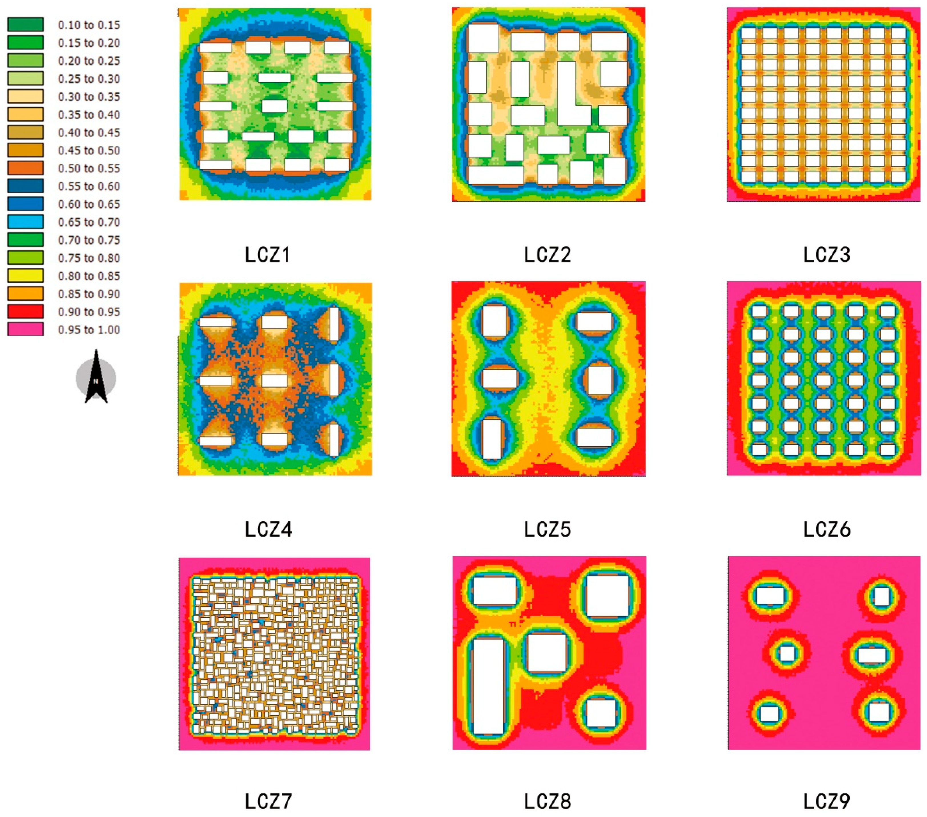
The SVF distribution of all nine models is shown in Figure 3. It can be seen from the maps that SVF gets smaller in the area near buildings. Comparing maps of LCZ1 and LCZ4 (same building height, but different building density and SVF), LCZ3 and LCZ6 (same building height, but different building density and SVF), it can be seen that the influencing area of buildings on SVF is related to the layout of buildings and the distance between them. Comparing LCZ5 with LCZ8 (similar SVF, but different building height and density), it can be seen that it is also related to the height of the building. Comparing LCZ8 and LCZ9 (same building height and similar layout, but different building density and floor area, similar SVF), it can be seen that the horizontal building size have limited impact on the average SVF value of the model in total as long as the buildings are loosely distributed. However, while comparing them with LCZ6 (same building height, crowded layout, different floor area and SVF), in which affecting areas of single building overlap each other, the average value of SVF will be much different.
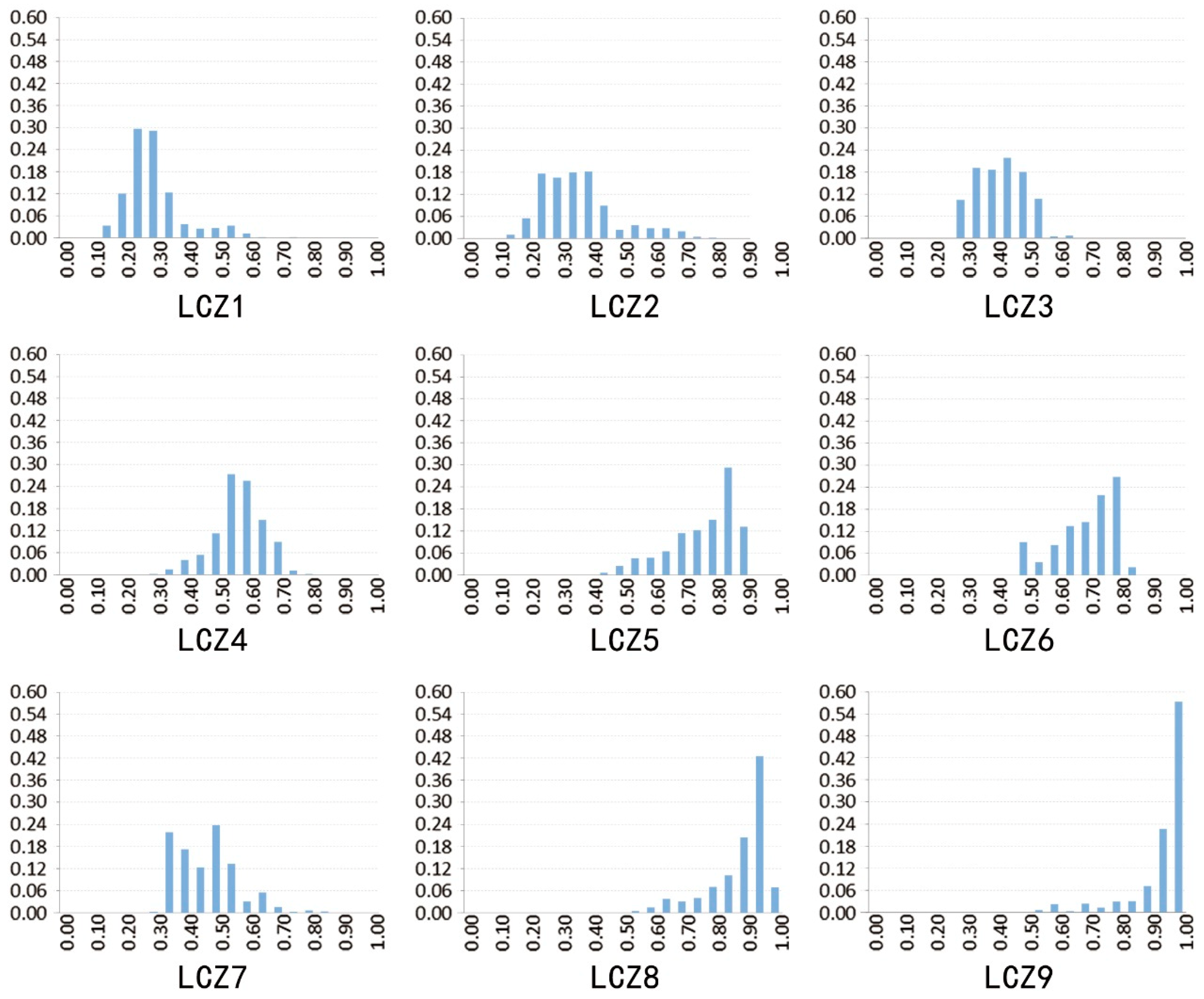
To better evaluate the SVF distribution and the effect of different morphological parameters (see Table 1), Figure 4 shows the statistical distribution of SVF for the nine models. LCZ1, 2, 3, and 7 (high-density models) show that SVF is mostly concentrated in the left part of the histograms. The SVF of LCZ6, which is characterized by a regular building layout and the same building height as LCZ3, is also concentrated but in the right part since it is characterized by a building density lower than LCZ3. Comparing the high-rise models LCZ1 and LCZ4, the lower density model LCZ4 shows larger SVF values. For low-rise, low-density models LCZ8 and LCZ9, most of the ground is not affected by the surrounding buildings, and the SVF values are concentrated in the second part of the histogram showing the largest values among the nine models investigated. According to the description of building density in Table 1, it can be thus noted that the height and the layout of buildings can affect the value of surrounding SVF to a great extent according to the SVF distribution of similar density models LCZ1 and LCZ6, as well as LCZ1 and LCZ8.

4.2. Spatial Distribution of MRT and PMV

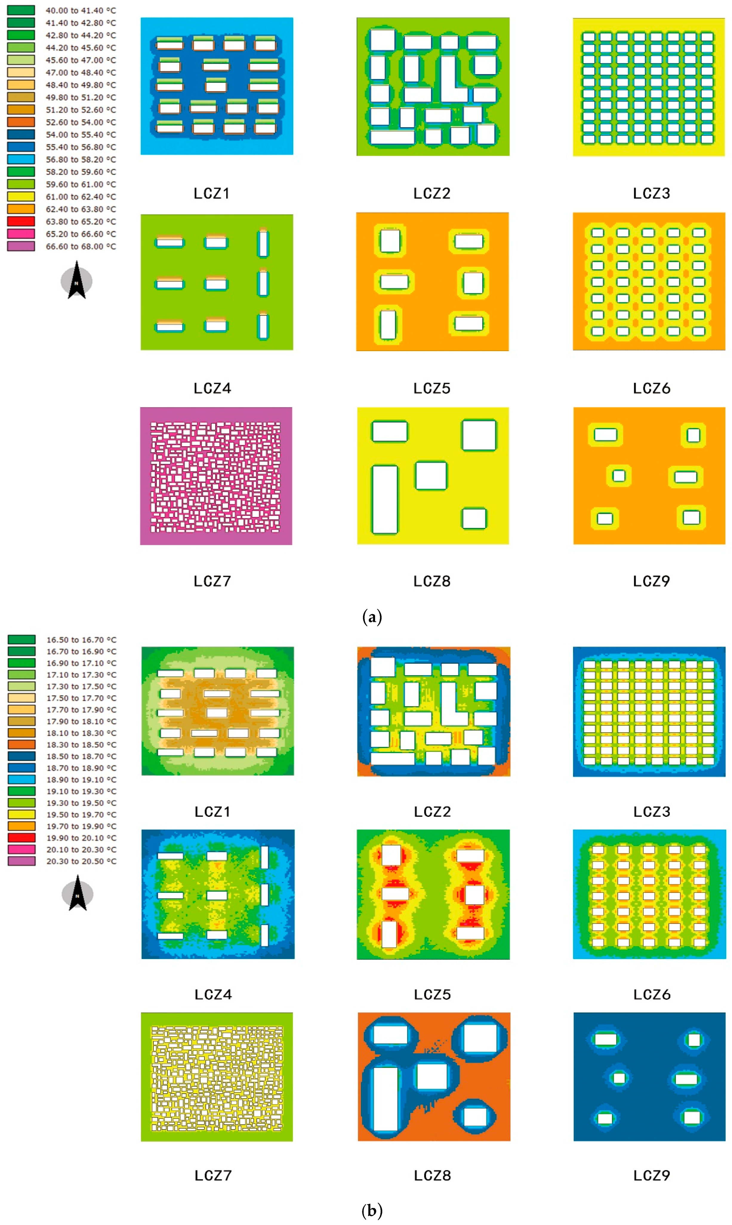
Figure 5 shows the MRT distribution maps at 12:00 (maximum solar radiation) and 21:00 (after sunset). The distribution of MRT follows the results of surface temperature (ST) (not shown here). In particular, during the day it is mainly affected by direct solar radiation, forming a distinct low temperature shadow area on the back of the buildings and this area is highly correlated with the building height. In particular, the high-rise models LCZ1 and LCZ4 (with a building height of 100 m) have bigger shadows than low-rise ones such as LCZ7 (with a building height of 4 m). During the night the MRT distribution is strongly correlated with the SVF distribution. Specifically, the lower the SVF, the higher the MRT. This is because when there is no radiation, the heat is released and reflected between surfaces in the form of long-wave radiation. In this situation, MRT is related to the visible area and temperature of the surrounding surface. Lower SVF areas represent denser buildings with larger surface area.
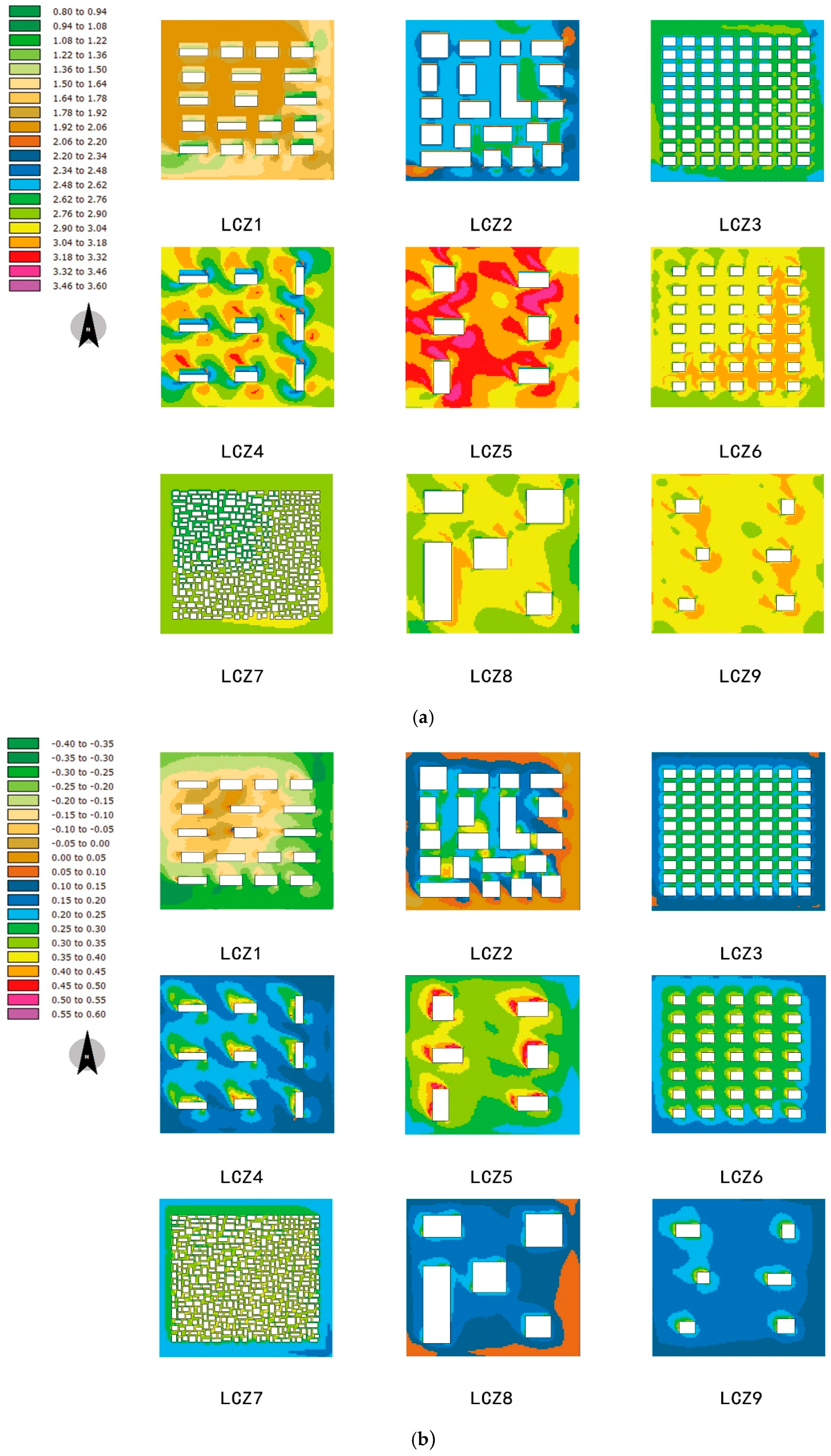
As a comprehensive index to describe human comfort, PMV, by definition, is closely related to AT, WS, RH, MRT, and other subjective parameters. Figure 6 shows the PMV distribution of nine models at 12:00 and 21:00. The distribution of PMV is similar to that of MRT, but it is greatly affected by WS, so a direct relationship between PMV and SVF (as for MRT) cannot be retrieved. Furthermore, WS is greatly influenced by the height, scale, and direction of the building, thus, no obvious correlation with the distribution of SVF occurs.
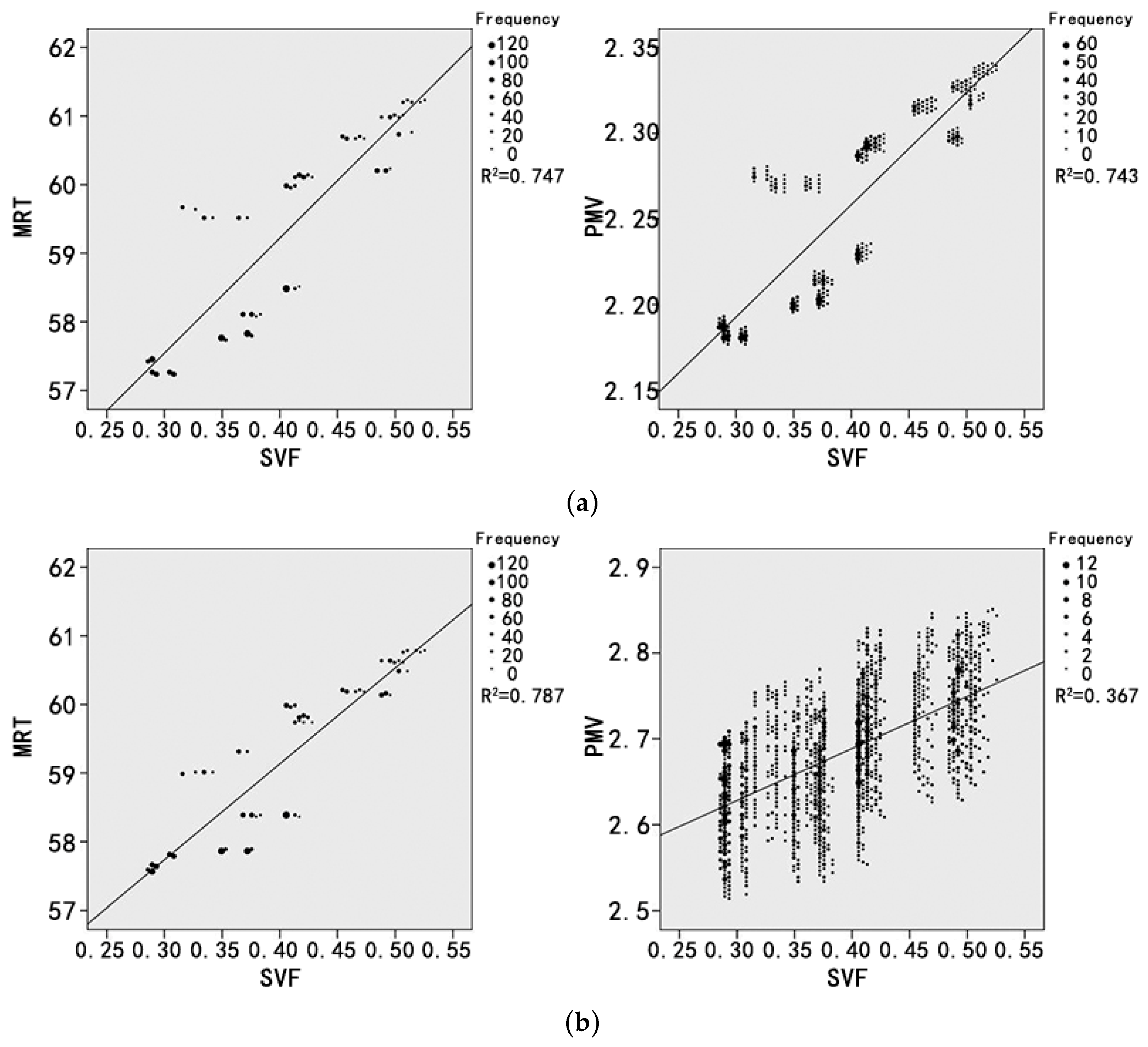
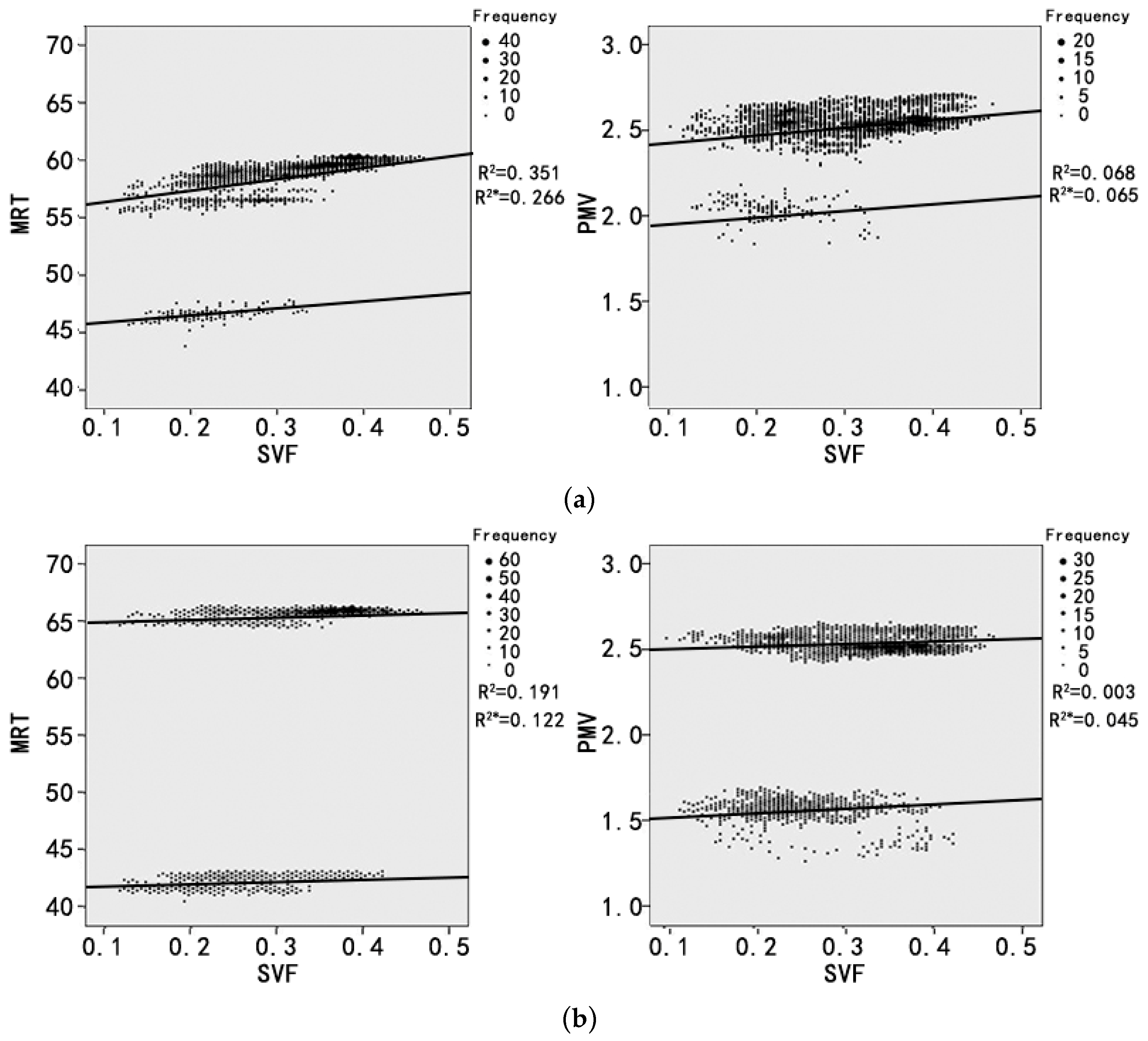
To show the impact of wind speed on PMV, LCZ3 is taken as an example due to its regular layout and wind speed pattern (not shown here). A simulation with initial wind speed WS of 0.5 m/s is thus performed and the correlation between MRT, PMV, and SVF at 12:00 is shown in Figure 7 in which the sizes of dots indicate the counts of data in the statistical units. WS has little effect on the relationship between SVF and MRT. The overall MRT with wind speed of 0.5 m/s is about 1 °C higher than that with wind speed of 3 m/s. The reason is that the heat exchange driven by the higher wind speed affects the surface temperature of buildings and ground in the area, which in turn has a certain impact on the long-wave radiation. However, this impact is not great enough to make a difference on the correlation. On the other hand, when wind speed is reduced, the correlation between SVF and PMV is similar to that of SVF and MRT, and its correlation coefficient is much higher than that of simulation under high wind speed. Therefore, it can be concluded that PMV and SVF have a stronger correlation at low wind speed, and this correlation is similar to that between MRT and SVF. It is worth noting that the two wind speeds considered are the speeds of the approaching wind imposed at the inlet boundary. When the wind, which is oblique, interacts with the geometry, it creates stagnation zones which are stronger at higher velocity and locally affect all the microclimate parameters involved in the PMV calculation. This in turn leads to a slight increase and an inhomogeneous distribution of PMV.

4.3. Correlation between SVF and Microclimate/Thermal Comfort Indices

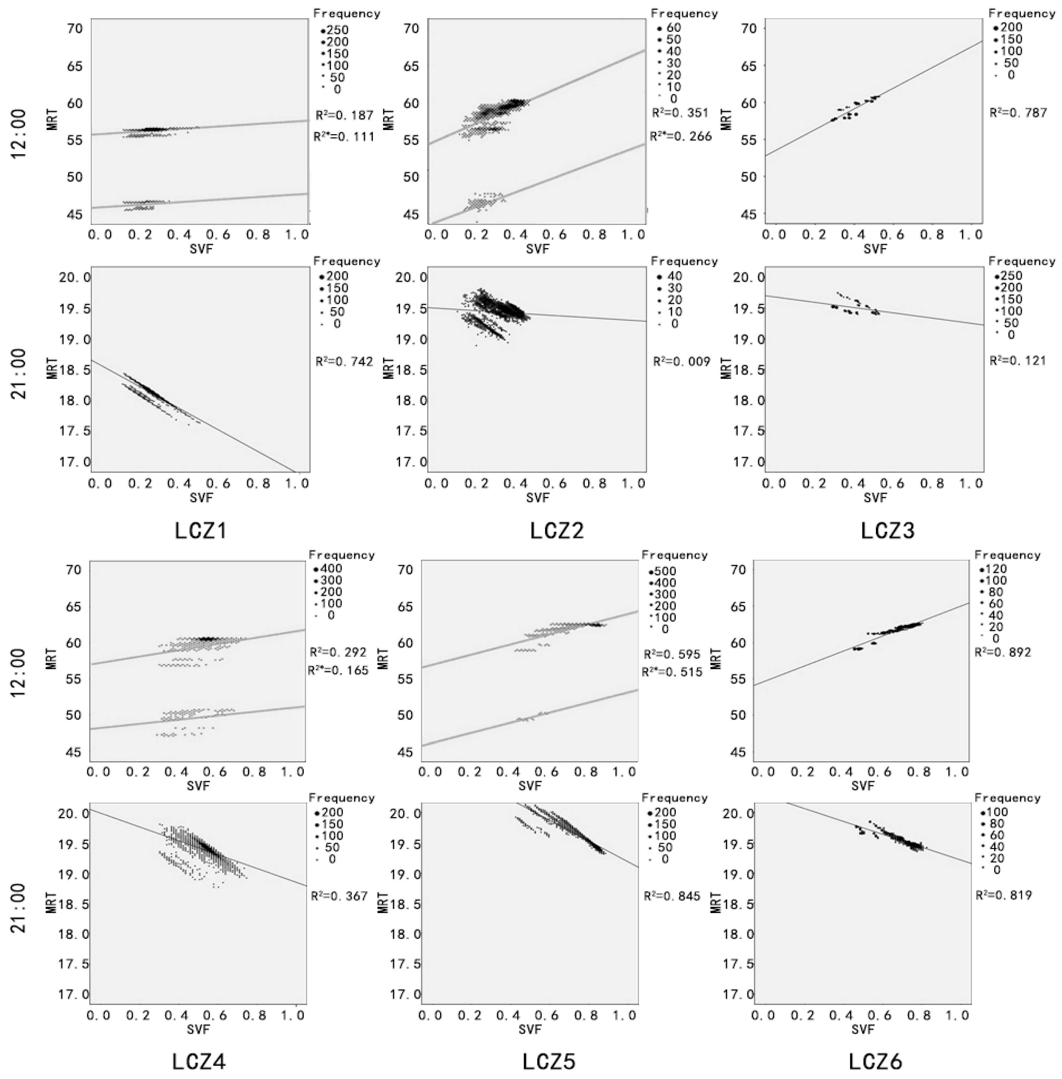
As suggested from the figures above (Figure 6 and Figure 8), the MRT distribution shows a certain correlation with SVF. Thus, as a next step, such correlation is quantitatively explored for all the nine models (Figure 8). As observed from the maps above, there is a strong negative correlation between SVF and MRT at 21:00, that is, the lower the SVF is, the higher the MRT will be. That is because a lower SVF indicates a higher long-wave radiation due to the reflection by the building surfaces. It is also claimed that there is a strong positive correlation between MRT and SVF at 12:00 during the day, and LCZ7 shows the strongest one. Except LCZ7, it is evident that MRT values are divided into two regions, which are more evident in LCZ1 and LCZ4 than in LCZ8 and LCZ9. This difference was due to the synergy between direct solar radiation and building height, which forms a direct-radiation area and a shadow area with lower MRT values. The higher the building is, the larger the shadow area is, and the more evident the two regions are.
In addition to the influence of building height on the size of shadow area in MRT distribution, the performance of different models in correlation is different, and this performance shows the same trend in daytime and night. As shown in Figure 8, the distribution of points in LCZ2, 3, and 4 is looser, showing less correlation between MRT and SVF distribution. Furthermore, for LCZ3, 6, 7, 8, and 9, which are all low-rise models, their correlation performance at 12:00 is more in line with the conclusion of positive correlation than other models. Finally, comparing the SVF intervals of each model and the corresponding correlation coefficients, models with a high correlation coefficient such as LCZ5, 6, 8, and 9 tend to have higher SVF values. It can be thus concluded that in the large SVF interval of 0.6–1, values of MRT at night have a high correlation with SVF. LCZ7, even though has a high correlation coefficient, shows medium SVF values since buildings are small and crowded.
Point-to-point correlation coefficients R between SVF and all the microclimate/thermal comfort indices are summarized in Table 3. Results quantitatively show that AT, RH, ST, and WS are not significantly correlated with SVF, while MRT and SVF are strongly negatively correlated during the night. PMV is not correlated with SVF in general, but there is a negative correlation in LCZ8 and 9 during the night. According to the results shown in Figure 7, the relationship between SVF and PMV is basically the same as that between SVF and MRT when wind speed has little influence. The relationship between PMV distribution in LCZ8 and 9 and their SVF is generally the same as MRT in most areas of the map since low building density and height contributed to small wind shadow area affected by wind speed. However, this conclusion does not apply to all models.
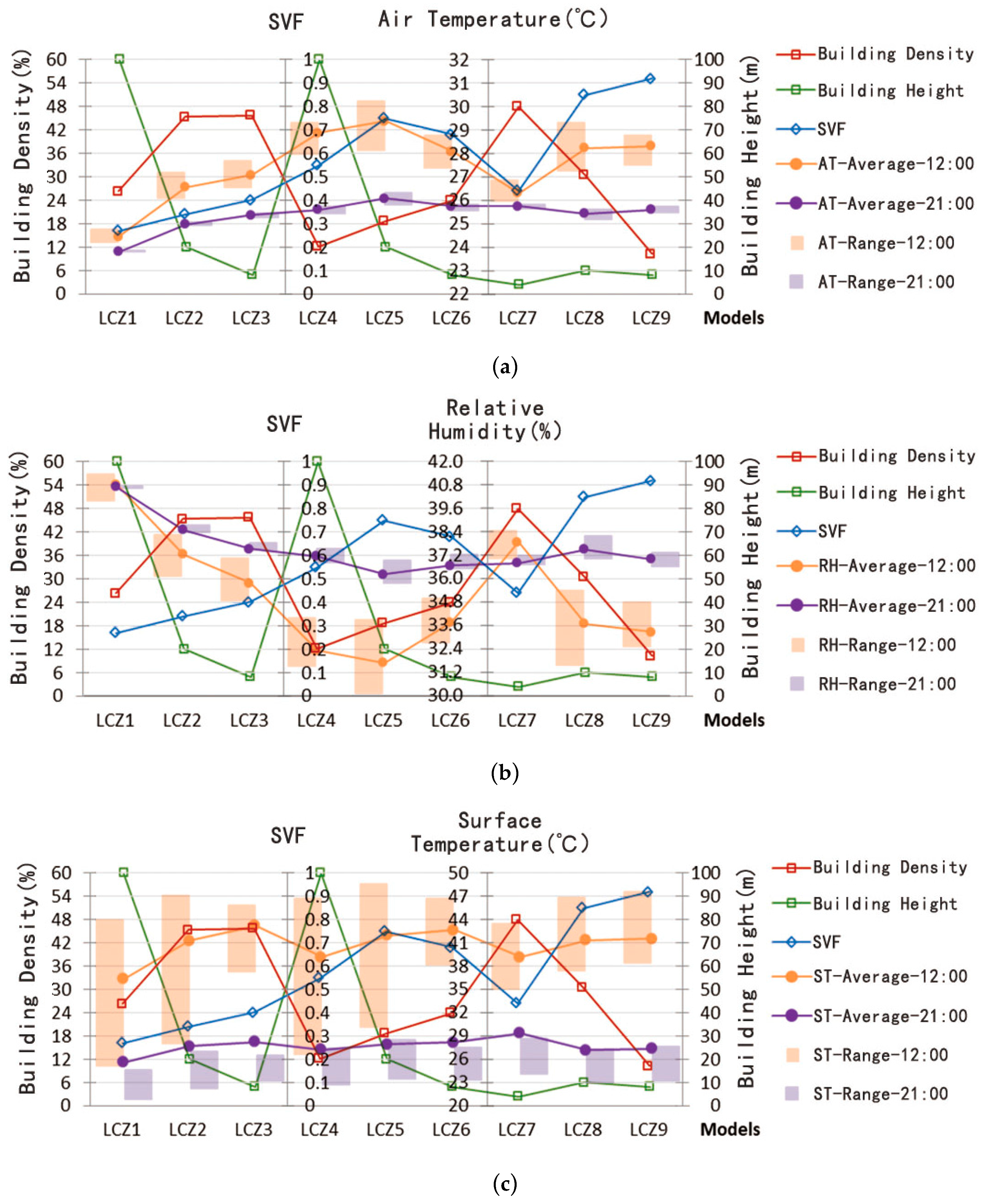
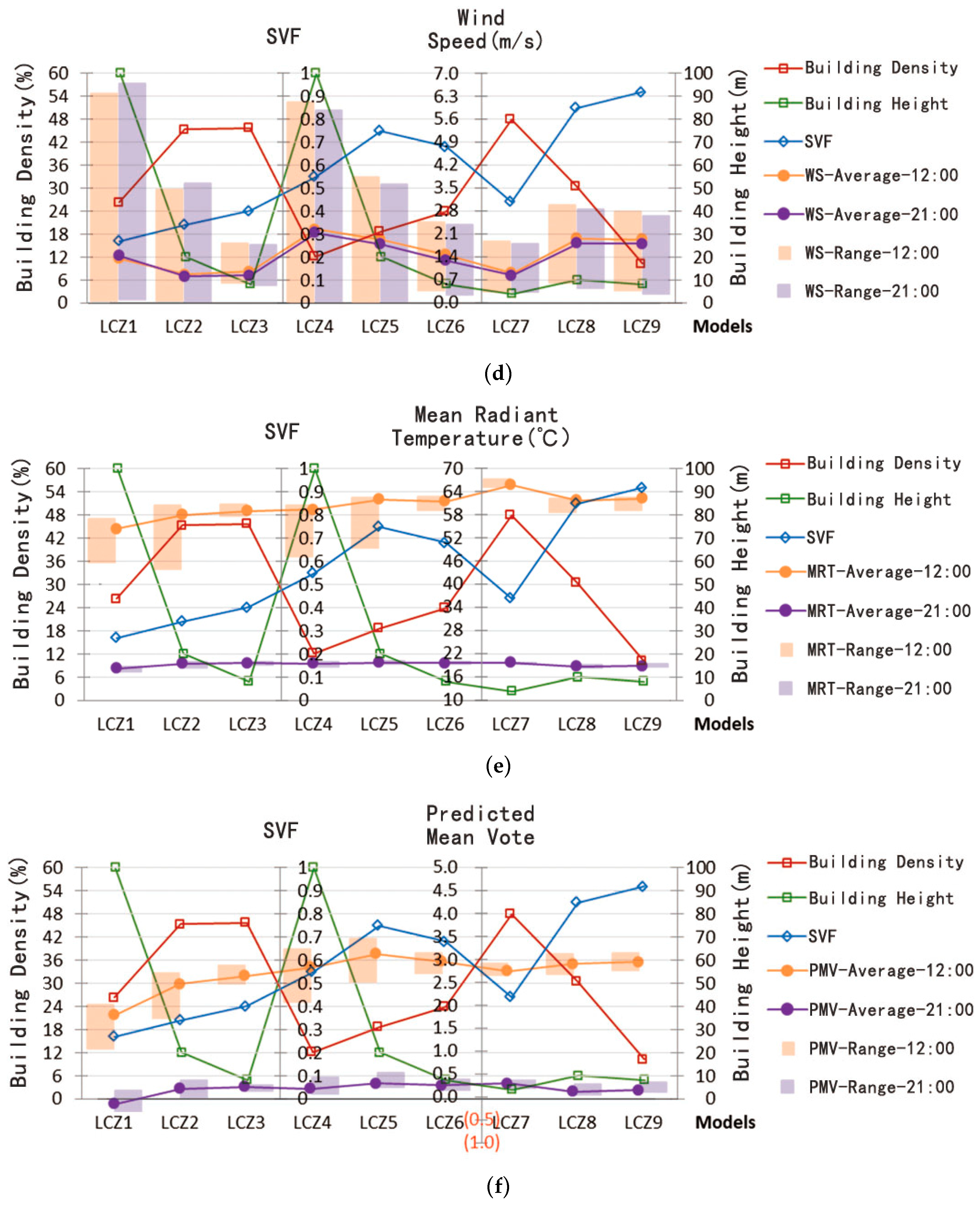
Figure 9 shows the profiles of spatially-averaged values of SVF and microclimate/thermal comfort indices for all the nine models. As can be seen from the figure, in general solar radiation has a great impact on values of all these indices except wind speed and leads to a higher range during the daytime than at night. For ST, WS, MRT, and PMV, the distribution range during the day is highly correlated with the building height. The higher the building, the more different conditions among the measured points on the map and the larger the ranges are. This conclusion is also applicable to the distribution of WS at night. Since factors such as plant and water were not considered, AT and RH showed an opposite trend. Further, from the overall analysis, significant correlation cannot be observed between the average MRT/PMV and SVF, but the average daytime AT and SVF show a high coincidence. There is also cause and effect and a negative correlation between the average value of building density and SVF in each model. Compact building groups tend to have a low average SVF value, but there might be other factors leading to changes in their relationship as can be seen from LCZ1–4. Moreover, the correlation between building density and microclimate indices is not evident.

4.4. Shadow Areas

As discussed above (see Figure 8), the scatter plots MRT–SVF during the day show two distinctive regions due to building shadow, and higher building groups tend to have larger shadow areas and more evident regions. Since the shadow area is also influenced by the latitude of the area, simulation results of Nanjing are compared with that of a place in Germany at 12:00 to confirm the dependence of MRT on the shadow area. Specifically, in ENVI-met the location of the model is changed to Germany, the latitude to 52.30 N and the longitude to 13.25 E, which ultimately affected the solar radiation since the solar incidence angle is increased. LCZ2 is taken as an example since at 12:00 it showed highly distinctive regions in the scatter plots and thus a proper comparison with the place in Germany is expected.
The scatter plots MRT–SVF and PMV–SVF are shown in Figure 10. The regions characterized by higher MRT values correspond to direct radiated areas, while the other regions (lower MRT values) correspond to the shadow areas. In Germany, as expected, if the solar incidence angle is increased, the shadow area is also increased and this corresponds to a larger gap between the two regions and to a large number of lower MRT values (as found for the higher building cases LCZ1 and 4). It can be concluded that a higher latitude has the same effect as of building height increase, which both lead to a larger shadow area. The relationship between PMV and SVF follows the same behavior as that for MRT.

5. Conclusions

In this paper, the correlation between the sky view factor (SVF) and six microclimate and thermal comfort indices (air temperature (AT), surface temperature (ST), wind speed (WS), mean radiant temperature (MRT), and predicted mean vote (PMV)) are studied for nine building models representing Local Climate Zone (LCZ) models through simulations with ENVI-met. The typical summer meteorological conditions of Nanjing were taken as boundary conditions. Main findings are summarized below:
  • The direct solar radiation strongly affects all the microclimate and thermal comfort indices except WS, and the correlation may differ in different models since height, density, and layout of buildings greatly affect shadow areas and wind patterns;
  • A strong point-to-point correlation between SVF and MRT is found. Specifically, the distribution of SVF and MRT is negatively correlated at night, while during the day the correlation is affected by the size of shadows formed by buildings: The greater the shadow, the stronger the correlation. Further, the correlation between MRT and SVF is increased for larger SVF values (in the interval of 0.6–1);
  • PMV is mainly determined by MRT under low wind speed and the point-to-point correlation with SVF follows a similar behavior to MRT, especially under low wind conditions;
  • In general, a clear correlation between spatially-averaged values of the indices and of SVF is not evident.
Overall, results suggest that the effect of urban morphology on microclimate and thermal comfort is local and cannot be retrieved using average values of morphological parameters and microclimate indices. On the other hand the comprehensive morphological parameter SVF, which simultaneously takes into account the effect of building height, layout, and density, seems to be appropriate to locally represent the effects of morphology on thermal comfort indices. There is still much left for future research in this paper, such as more comprehensive data comparison methods, a more detailed control and description of model variables, and the application to real urban cases.

Author Contributions

Conceptualization, Z.G.; methodology, T.L., R.B., and Z.G.; software, T.L.; formal analysis, T.L., R.B., and Z.G.; writing—original draft preparation, T.L.; writing—review and editing, R.B.; supervision, R.B. and Z.G.; project administration, Z.G.

Funding

The research was supported by the key project funded by the National Science Foundation of China on “Urban form-microclimate coupling mechanism and control”, Grant No. 51538005.

Conflicts of Interest

The authors declare no conflict of interest.

References

  1. Yang, L.; Qian, F.; Song, D.-X.; Zheng, K.-J. Research on Urban Heat-Island Effect. Procedia Eng. 2016, 169, 11–18. [Google Scholar] [CrossRef]
  2. Li, X.; Zhou, Y.; Yu, S.; Jia, G.; Li, H.; Li, W. Urban heat island impacts on building energy consumption: A review of approaches and findings. Energy 2019, 174, 407–419. [Google Scholar] [CrossRef]
  3. Hankey, S.; Marshall, J.D. Urban Form, Air Pollution, and Health. Curr. Environ. Health Rep. 2017, 4, 491–503. [Google Scholar] [CrossRef] [PubMed]
  4. Maucieri, C.; Barbera, A.C.; Vymazal, J.; Borin, M. A review on the main affecting factors of greenhouse gases emission in constructed wetlands. Agric. For. Meteorol. 2017, 236, 175–193. [Google Scholar] [CrossRef]
  5. Lin, P.; Gou, A.; Lau, S.S.-Y.; Qin, H. The impact of urban design descriptors on outdoor thermal environment: A literature review. Energies 2017, 10, 2151. [Google Scholar] [CrossRef]
  6. Nowak, D.J. The atmospheric system: Air quality and greenhouse gases. In Understanding Urban Ecology; Hall, M.H.P., Balough, S.B., Eds.; Springer Nature: Basel, Switzerland, 2019; pp. 175–199. [Google Scholar]
  7. Yang, Y.; Gatto, E.; Gao, Z.; Buccolieri, R.; Morakinyo, T.E.; Lan, H. The “plant evaluation model” for the assessment of the impact of vegetation on outdoor microclimate in the urban environment. Build. Environ. 2019, 159, 106151. [Google Scholar] [CrossRef]
  8. Toparlar, Y.; Blocken, B.; Maiheu, B. A review on the CFD analysis of urban microclimate. Renew. Sustain. Energy Rev. 2017, 80, 1613–1640. [Google Scholar] [CrossRef]
  9. Hazim, B. Awbi, Ventilation of Building; Taylor & Francis Ltd.: Didcott, UK, 2003. [Google Scholar]
  10. Honjo, T. Thermal Comfort in Outdoor Environment. Glob. Environ. Res. 2009, 13, 43–47. [Google Scholar]
  11. Mukherjee, M.; Mahanta, S. Outdoor thermal comfort: A review on the concepts, parameters and methods to evaluate thermal comfort in outdoor space. Archit.-Time Space People 2014, 16–22. Available online: https://www.coa.gov.in/show_img.php?fid=109 (accessed on 27 June 2019).
  12. Chen, L.; Ng, E. Outdoor thermal comfort and outdoor activities: A review of research in the past decade. Cities 2012, 29, 118–125. [Google Scholar] [CrossRef]
  13. Walls, W.; Parker, N.; Walliss, J. Designing with thermal comfort indices in outdoor sites. In Living and Learning: Research for a Better Built Environment: 49th International Conference of the Architectural Science Association; Crawford, R.H., Stephan, A., Eds.; The Architectural Science Association and The University of Melbourne: Melbourne, Australia, 2015; pp. 1117–1128. [Google Scholar]
  14. Di Sabatino, S.; Buccolieri, R.; Kumar, P. Spatial distribution of air pollution in cities. In Clinical Handbook of Air Pollution-Related Diseases; Capello, F., Gaddi, A., Eds.; Springer: Cham, Switzerland, 2018; pp. 75–95. [Google Scholar]
  15. Buccolieri, R.; Hang, J. Recent advances in urban ventilation assessment and flow modelling. Atmosphere 2019, 10, 144. [Google Scholar] [CrossRef]
  16. Oke, T.R. Canyon geometry and the nocturnal urban heat island: Comparison of scale model and field observations. J. Climatol. 1981, 1, 237–254. [Google Scholar] [CrossRef]
  17. Stewart, I.D. Local climate zones: Origins, development, and application to urban heat island studies. In Proceedings of the Annual Meeting of the American Association of Geographers, Seattle, WA, USA, 11–16 April 2011. [Google Scholar]
  18. Stewart, I.D.; Oke, T.R. Local Climate Zones for Urban Temperature Studies. Bull. Am. Meteorol. Soc. 2012, 93, 1879–1900. [Google Scholar] [CrossRef]
  19. Jamei, E.; Rajagopalan, P.; Seyedmahmoudian, M. Review on the impact of urban geometry and pedestrian level greening on outdoor thermal comfort. Renew. Sustain. Energy Rev. 2016, 54, 1002–1017. [Google Scholar] [CrossRef]
  20. Hien, W.N.; Jusuf, S.K. Air Temperature Distribution and the Influence of Sky View Factor in a Green Singapore Estate. J. Urban Plan. Dev. 2010, 136, 261–272. [Google Scholar] [CrossRef]
  21. He, X.; Miao, S.; Shen, S. Influence of sky view factor on outdoor thermal environment and physiological equivalent temperature. Int. J. Biometeorol. 2015, 59, 285–297. [Google Scholar] [CrossRef]
  22. Wang, Y.; Akbari, H. Effect of Sky View Factor on Outdoor Temperature and Comfort in Montreal. Environ. Eng. Sci. 2014, 31, 272–287. [Google Scholar] [CrossRef]
  23. Feng, Y.; Feng, Q.; Lau, S.S. Urban form and density as indicators for summertime outdoor ventilation potential: A case study on high-rise housing in Shanghai. Build. Environ. 2013, 70, 122–137. [Google Scholar]
  24. Unger, J. Intra-urban relationship between surface geometry and urban heat island: Review and new approach. Clim. Res. 2004, 27, 253–264. [Google Scholar] [CrossRef]
  25. Oke, T.R.; Johnson, G.T.; Steyn, D.G.; Watson, I.D. Simulation of surface urban heat islands under ‘ideal’ conditions at night part 2: Diagnosis of causation. Bound.-Layer Meteorol. 1991, 56, 339–358. [Google Scholar] [CrossRef]
  26. Park, H.S. Variations in the Urban Heat Island Intensity Affected by Geographical Environments. Ph.D. Thesis, University of Tsukuba, Tsukuba, Japan, 1987. [Google Scholar]
  27. Chen, L.; Ng, E.; An, X.; Ren, C.; Lee, M.; Wang, U.; He, Z. Sky view factor analysis of street canyons and its implications for daytime intra-urban air temperature differentials in high-rise, high-density urban areas of Hong Kong: A GIS-based simulation approach. Int. J. Climatol. 2012, 32, 121–136. [Google Scholar] [CrossRef]
  28. Chao, Y.; Liang, C. Mitigating urban heat island effects in high-density cities based on sky view factor and urban morphological understanding: A study of Hong Kong. Archit. Sci. Rev. 2011, 54, 305–315. [Google Scholar]
  29. Unger, J. Connection between urban heat island and sky view factor approximated by a software tool on a 3D urban database. Int. J. Environ. Pollut. 2009, 363, 59–80. [Google Scholar] [CrossRef]
  30. Stewart, I.D.; Oke, T.R.; Krayenhoff, E.S. Evaluation of the ‘local climate zone’ scheme using temperature observations and model simulations. Int. J. Climatol. 2014, 34, 1062–1080. [Google Scholar] [CrossRef]
  31. Lelovics, E.; Unger, J.; Gal, T. Design of an urban monitoring network based on Local Climate Zone mapping and temperature pattern modelling. Clim. Res. 2014, 60, 51–62. [Google Scholar] [CrossRef]
  32. Gal, T.; Benjamin, B.; Janos, U. Comparison of two different Local Climate Zone mapping methods. In Proceedings of the 9th International Conference on Urban Climate, Toulouse, France, 20–24 July 2015. [Google Scholar]
  33. Bechtel, B.; Daneke, C. Classification of Local Climate Zones Based on Multiple Earth Observation Data. IEEE J. Sel. Top. Appl. Earth Obs. Remote. Sens. 2012, 5, 1191–1202. [Google Scholar] [CrossRef]
  34. Ng, E.; Yuan, C.; Chen, L. Improving the wind environment in high-density cities by understanding urban morphology and surface roughness: A study in Hong Kong. Landsc. Urban Plan. 2011, 101, 59–74. [Google Scholar] [CrossRef]
  35. Bechtel, B.; Alexander, P.J.; Bhner, J. Mapping Local Climate Zones for a Worldwide Database of the Form and Function of Cities. ISPRS Int. J. Geo-Inf. 2015, 4, 199–219. [Google Scholar] [CrossRef] [Green Version]
  36. Huttner, S. Further Develop and Application of the 3D Microclimate Simulation ENVI-met. Ph.D. Thesis, Johannes Gutenberg-University, Mainz, Germany, 2012. Available online: https://publications.ub.uni-mainz.de/theses/volltexte/2012/3112/pdf/3112.pdf (accessed on 19 July 2019).
  37. Simon, H. Modeling Urban Microclimate. Development, Implementation and Evaluation of New and Improved Calculation Methods for the Urban Microclimate Model ENVI-Met. Johannes Gutenberg-University in Mainz 2016. Available online: https://publications.ub.uni-mainz.de/theses/volltexte/2016/100000507/pdf/100000507.pdf (accessed on 19 July 2019).
  38. Tsoka, S.; Tsikaloudaki, A.; Theodosiou, T. Analyzing the ENVI-met microclimate model’s performance and assessing cool materials and urban vegetation applications–A review. Sustain. Cities Soc. 2018, 43, 55–76. [Google Scholar] [CrossRef]
  39. Hoppe, P. The physiological equivalent temperature–A universal index for the biometeorological assessment of the thermal environment. Int. J. Biometeorol. 1999, 43, 71–75. [Google Scholar] [CrossRef]
  40. Qaid, A.; Lamit, H.B.; Ossen, D.R.; Shahminan, R.N.R. Urban heat island and thermal comfort conditions at micro-climate scale in a tropical planned city. Energy Build. 2016, 133, 577–595. [Google Scholar] [CrossRef]
  41. Rui, L.; Buccolieri, R.; Zhi, G.; Gatto, E.; Ding, W. Study of the effect of green quantity and structure on thermal comfort and air quality in an urban-like residential district by ENVI-met modelling. Build. Simul. 2019, 12, 183–194. [Google Scholar] [CrossRef]
  42. Fanger, P.O. Thermal Comfort: Analysis and Applications in Environmental Engineering; Danmarks Tekniske H Jskole: Copenhagen, Denmark, 1970. [Google Scholar]
  43. Jendritzky, G.; Nübler, W. A model analysing the urban thermal environment in physiologically significant terms. Arch. Meteorol. Geophys. Bioclimatol. Ser. B 1981, 29, 313–326. [Google Scholar] [CrossRef]
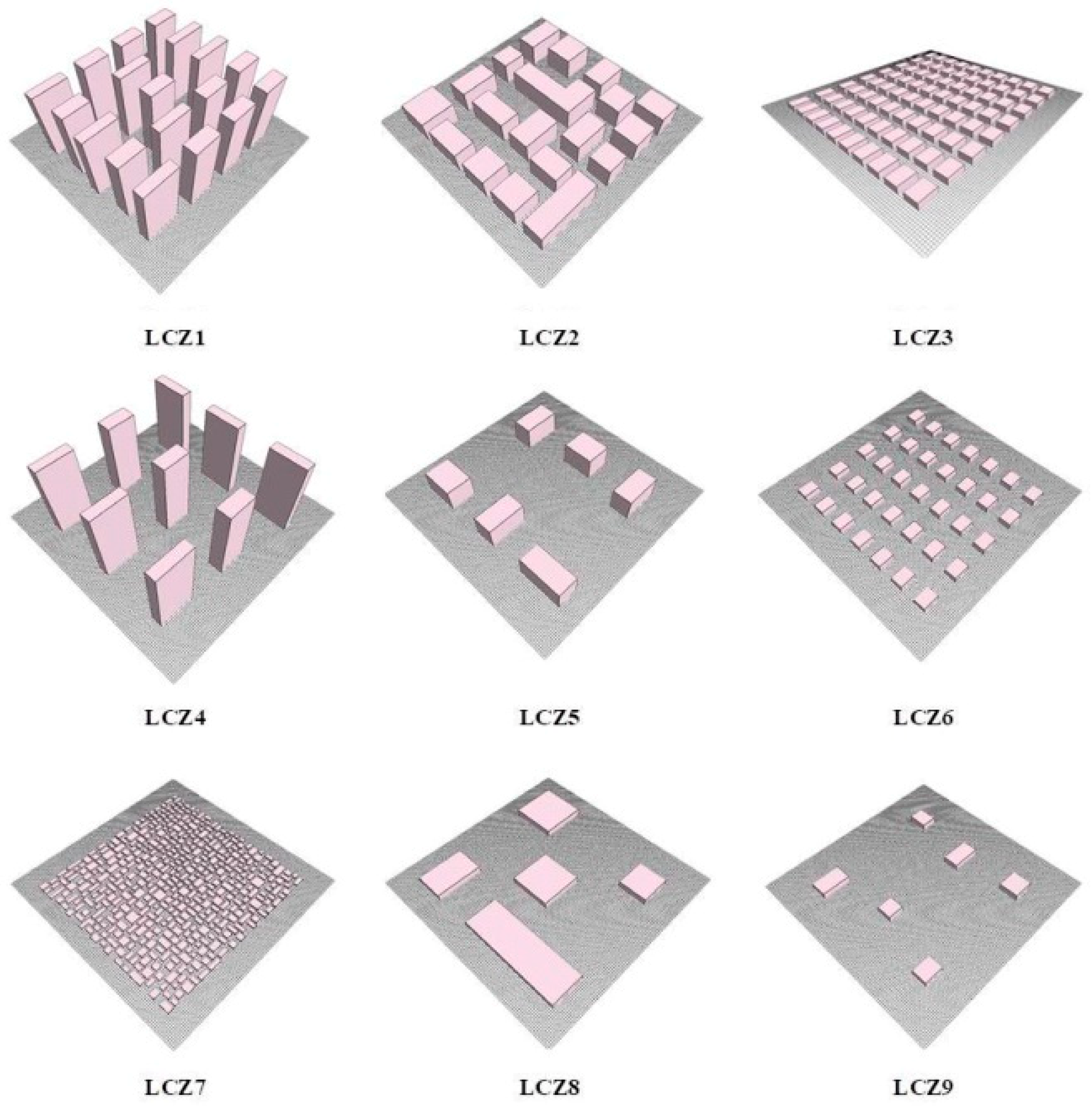
Figure 1. Investigated ideal block models following Local Climate Zone (LCZ) 1–9 classification.
Atmosphere 10 00438 g001
Figure 2. Satellite images of different districts in Nanjing. (a) Yile, Living community—compact mid-rise, LCZ2; (b) Xinjiekou, Commercial center—open high-rise LCZ4; (c) Menxi, Historical living zone—lightweight low-rise, LCZ7.
Atmosphere 10 00438 g002
Figure 3. Spatial distribution of the sky view factor (SVF) for all the nine models.
Atmosphere 10 00438 g003
Figure 4. Statistical distribution of SVF for all the nine models.
Atmosphere 10 00438 g004
Figure 5. Distribution of mean radiant temperature (MRT) at 12:00 (a) and 21:00 (b) for all the nine models.
Atmosphere 10 00438 g005
Figure 6. Distribution of predicted mean vote (PMV) at 12:00 (a) and 21:00 (b) for all the nine models.
Atmosphere 10 00438 g006
Figure 7. Correlation between SVF and MRT/PMV of the model LCZ3 at 12:00 with (a) WS = 0.5 m/s and (b) WS = 3 m/s.
Atmosphere 10 00438 g007
Figure 8. Correlation between SVF and MRT for the nine models at 12:00 and 21:00, with indication of the square of the correlation coefficient R2. Please note that, when two values of R2 are present, R2 refers to the direct-radiation area and R2* to the shadow area.
Atmosphere 10 00438 g008aAtmosphere 10 00438 g008b
Figure 9. Comparison between SVF and microclimate and thermal comfort indices for all the nine models. (a) air temperature, (b) relative humidity, (c) surface temperature, (d) wind speed, (e) mean radiant temperature, (f) predicted mean vote.
Atmosphere 10 00438 g009aAtmosphere 10 00438 g009b
Figure 10. Correlation between SVF and MRT/PMV for LCZ2 at 12:00 in (a) Nanjing and (b) Germany, with indication of the square of the correlation coefficient R2. Please note that R2 refers to the direct-radiation area and R2* to the shadow area.
Atmosphere 10 00438 g010
Table 1. Parameters of the nine ideal city models (standards from Stewart et al. [30]).
LCZ1LCZ2LCZ3LCZ4LCZ5LCZ6LCZ7LCZ8LCZ9
LCZ typeCompact high-riseCompact mid-riseCompact low-riseOpen high-riseOpen mid-riseOpen low-riseLightweight low-riseLarge low-riseSparsely built
Average height (m)1002081002084108
Average floor area (m2)8002200300800120030010036001200
Building density (%)26.345.445.712.118.723.94830.410.2
LCZ Standard density (%)40–6040–7040–7020–4020–4020–4060–9030–5010–20
Average SVF0.270.340.400.550.750.680.440.850.92
LCZ Standard SVF0.2–0.40.3–0.60.2–0.60.5–0.70.5–0.80.6–0.90.2–0.5>0.7>0.8
Table 2. Initial and boundary conditions used in ENVI-met simulations.
Parameter TypeParameter NameSettings
Location on earthName of locationNanjing
Position on earth118.78 E, 32.05 N
Time and dateStart date and start time23.06.2017, 6:00
Total simulation15 h
Initial meteorological conditionsWind speed measured in 10 m height3 m/s
Wind direction (0 = form North, 180 = from South)135 °
Roughness length at measurement site0.1
Initial temperature of atmosphere (2500 m)21 ℃
Specific humidity at model top 7 g/kg
Relative humidity in 2 m50%
Dynamic time stepTime step (solar angle ≥ 50 °) 1 s
Time step (solar angle < 50 °)2 s
Soil and vegetation conditionsInitial surface temperature of soil293 K
Initial surface relative humidity of soil50%
Vegetation transpiration modelA-gs Photosyntesis
CO2 background concentration350 ppm
Turbulence model and later boundary conditionsTurbulence modelStandard TKE Model (Mellor and Yamada 1982)
Lateral boundary conditionsCyclic
Personal human parametersAge of person, gender 35 years, male
Height, weight175 cm, 70 kg
Static clothing insulation0.9 clo
Total metabolic rate80 W/m2
Table 3. Correlation coefficients R between SVF and the microclimate/thermal comfort indices for all the nine models. Please note that, when two values are present, * refers to the shadow area.
ModelTimeATSTRHWSMRTPMV
LCZ112:00−0.900/−0.287 *−0.342/−0.249*0.131/0.361 *0.270/0.221 *0.392/0.310 *−0.351/−0.268 *
21:00−0.3350.2730.0840.002−0.947−0.029
LCZ212:00−0.124/−0.069*−0.042/0.006 *0.171/0.471 *0.462/0.124 *0.543/0.500 *0.038/−0.254 *
21:00−0.079−0.067−0.0860.231−0.659−0.319
LCZ312:000.043−0.039−0.1880.6540.8310.606
21:00−0.0680.131−0.4220.638−0.467−0.657
LCZ412:000.228/−0.155 *−0.020/0.237 *−0.186/0.201 *0.373/0.448 *0.495/0.404 *−0.198/−0.341*
21:00−0.2680.299−0.4770.5240.142−0.572
LCZ512:00−0.101/0.094 *−0.213/0.450 *0.102/0.128 *0.390/0.430 *0.733/0.739 *−0.101/−0.201 *
21:00−0.2770.232−0.4870.424−0.911−0.659
LCZ612:00−0.1050.125−0.2110.4580.9300.529
21:00−0.1830.112−0.3930.392−0.894−0.579
LCZ712:00−0.1040.1150.499−0.0530.9890.245
21:00−0.071−0.0020.299−0.059−0.989−0.032
LCZ812:00−0.0600.102−0.4820.6300.907−0.034
21:00−0.4390.441−0.5240.594−0.977−0.835
LCZ912:000.045−0.073−0.6080.7170.927−0.063
21:00−0.0590.021−0.6960.698−0.980−0.804