Occurrence and Coupling of Heat and Ozone Events and Their Relation to Mortality Rates in Berlin, Germany, between 2000 and 2014


Abstract
1. Introduction
2. Data and Methods
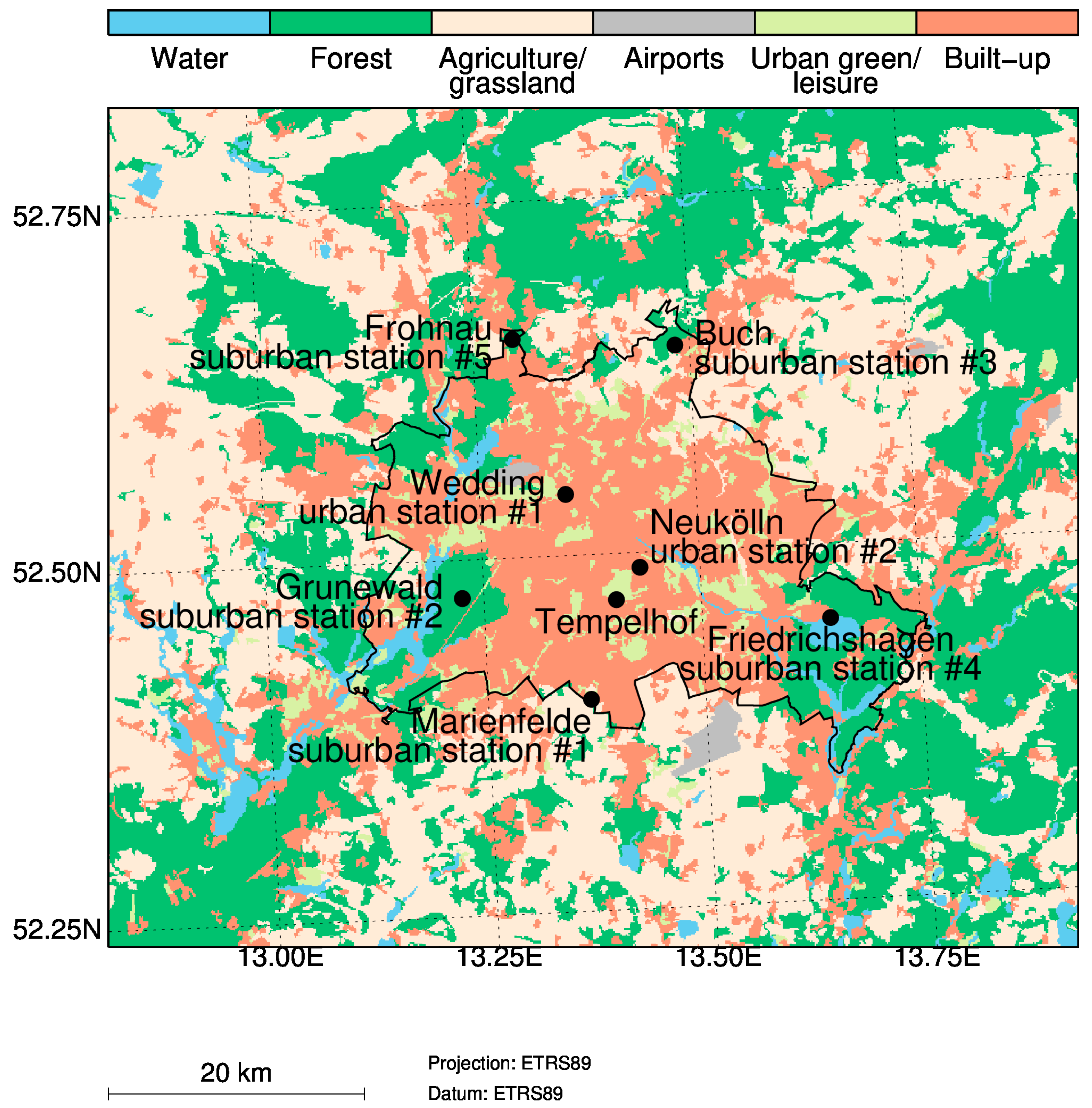
2.1. Study Area
2.2. Data
2.3. Methods
2.3.1. Event-Based Regressions
2.3.2. Selection of Event-Based Regressions
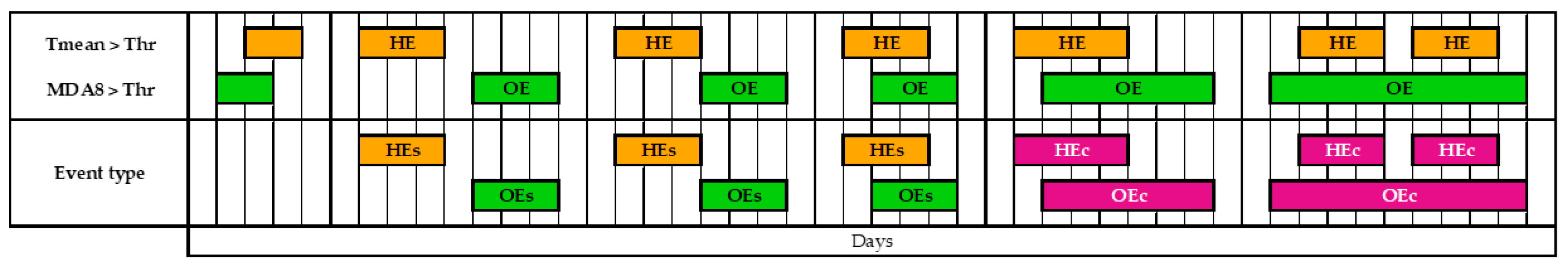
2.3.3. Classification of Single and Coupled Events
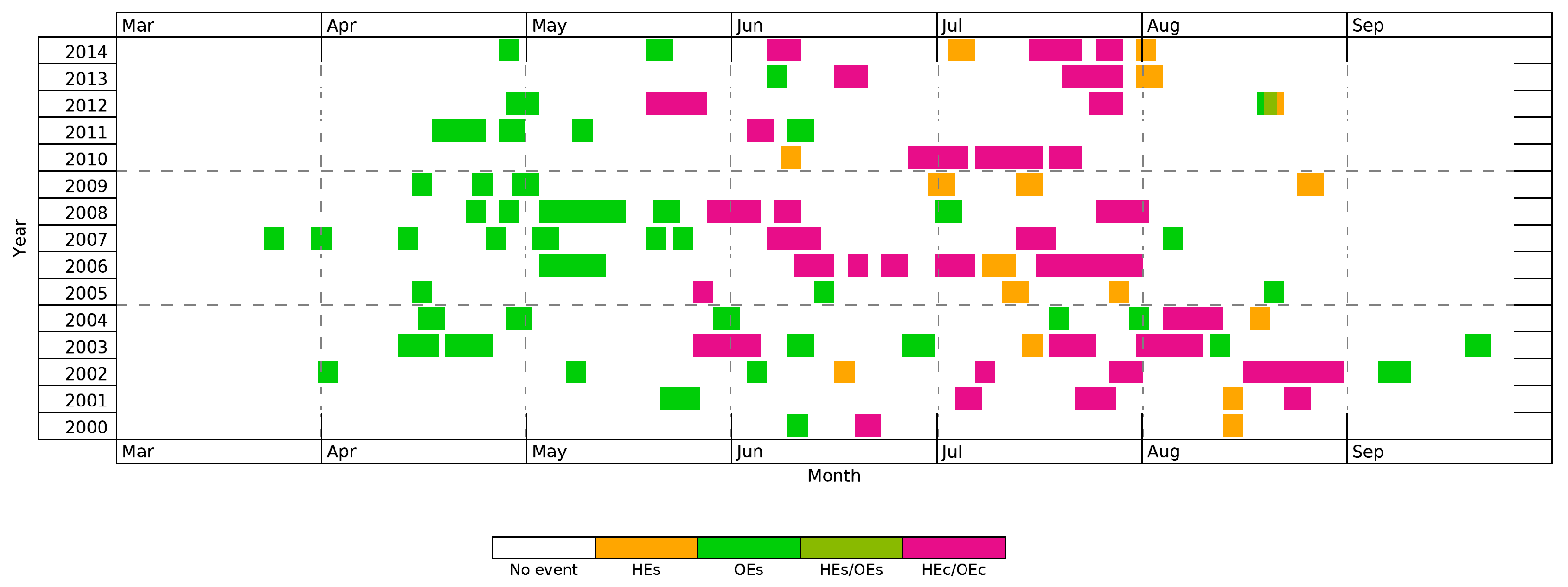
- Single heat events (HEs): Events of Tmean threshold exceedance for at least three consecutive days, and not more than two consecutive days of MDA8 threshold exceedance.
- Coupled heat event (HEc): Events of Tmean threshold exceedance for at least three consecutive days, and at least three consecutive days of MDA8 threshold exceedance.
- Single ozone events (OEs): Events of MDA8 threshold exceedance for at least three consecutive days, and not more than two consecutive days of Tmean threshold exceedance.
- Coupled ozone event (OEc): Events of MDA8 threshold exceedance for at least three consecutive days, and at least three consecutive days of Tmean threshold exceedance.
3. Results
3.1. Risk-Based Event Analysis
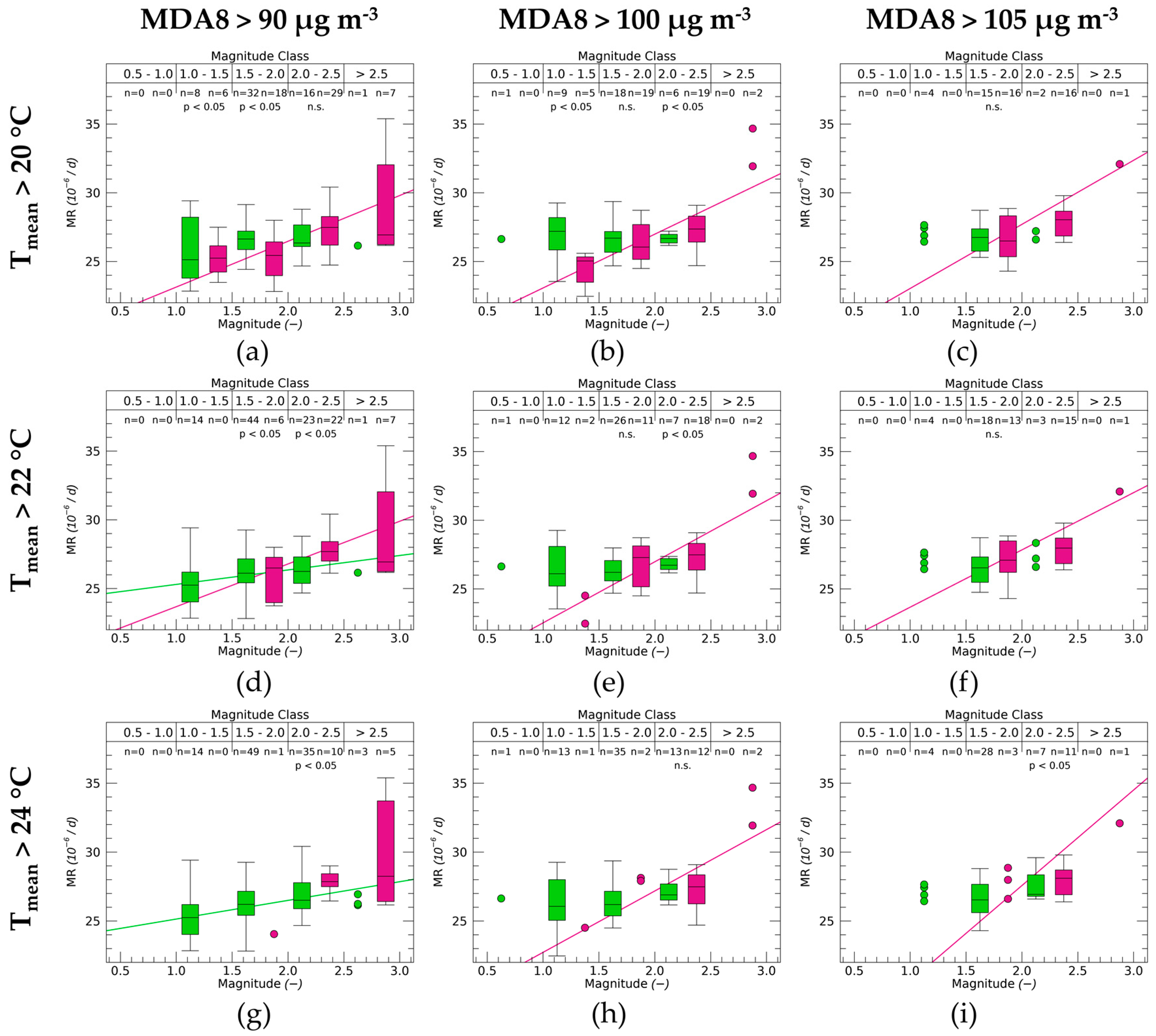
3.1.1. Air Temperature
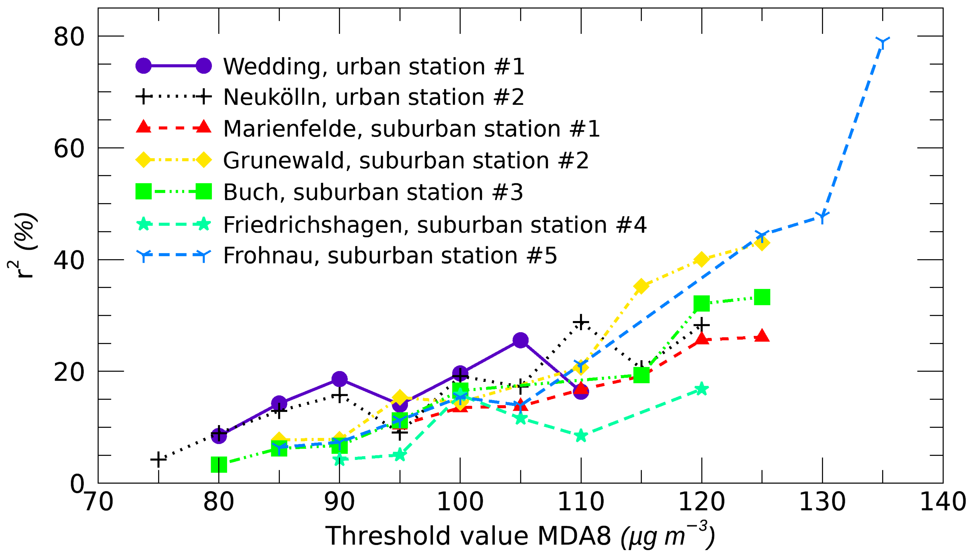
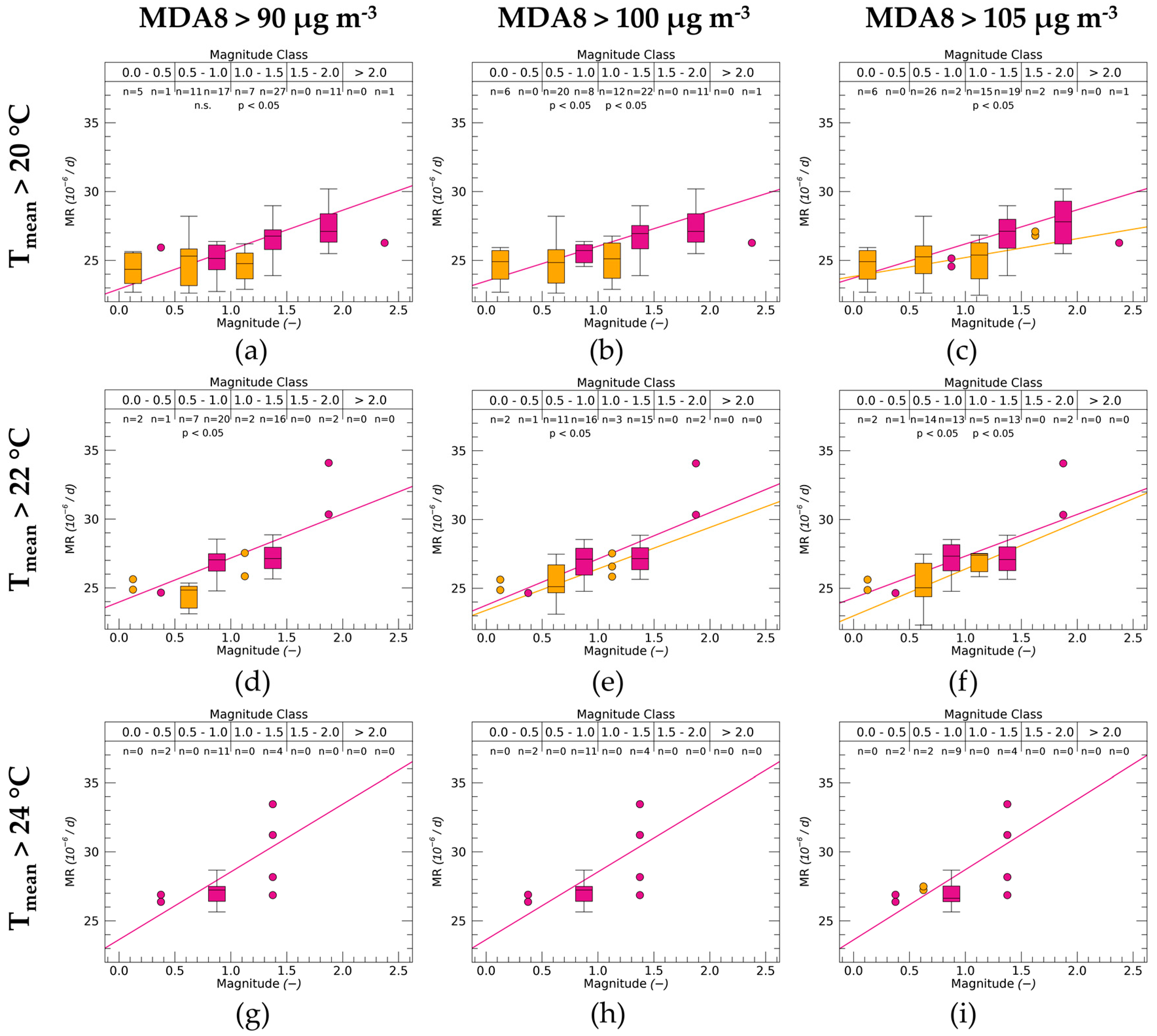
3.1.2. Ozone
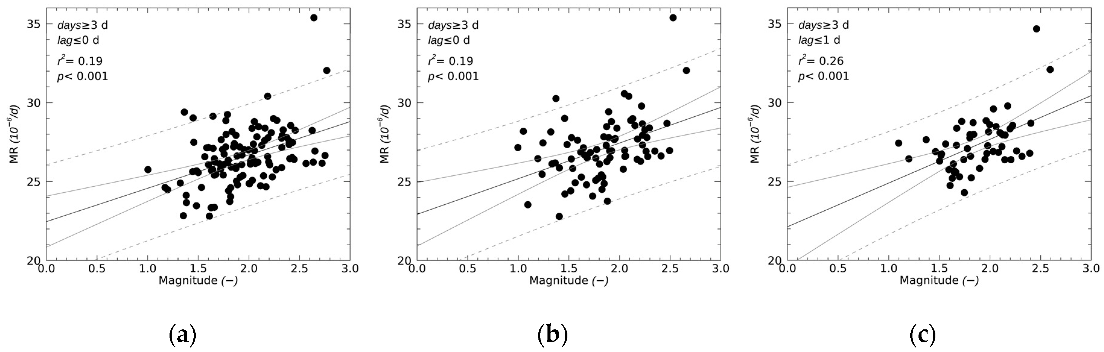
3.2. Event Type-Specific Mortality Rates
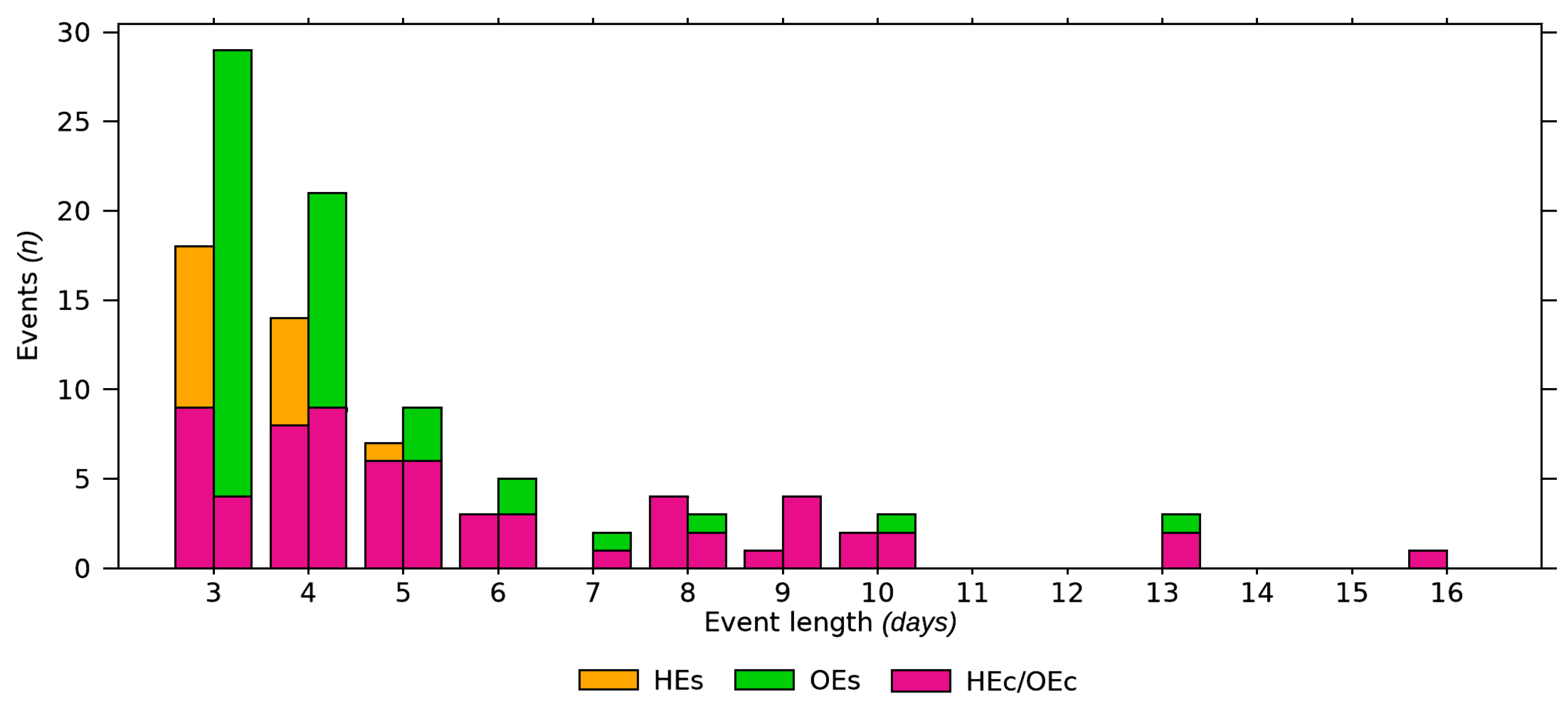
3.3. Temporal Pattern of Events
4. Discussion
4.1. Risk-Based Identification of Heat and Ozone Events
4.2. Influence of Ozone onto Heat Events
4.3. Influence of Air Temperature onto Ozone Events
5. Conclusions
Supplementary Materials
Author Contributions
Funding
Acknowledgments
Conflicts of Interest
References
- Tong, S.; Wang, X.Y.; FitzGerald, G.; McRae, D.; Neville, G.; Tippett, V.; Aitken, P.; Verrall, K. Development of health risk-based metrics for defining a heatwave: A time series study in Brisbane, Australia. BMC Public Health 2014, 14, 435. [Google Scholar] [CrossRef] [PubMed]
- Williams, S.; Nitschke, M.; Sullivan, T.; Tucker, G.R.; Weinstein, P.; Pisaniello, D.L.; Parton, K.A.; Bi, P. Heat and health in Adelaide, South Australia: Assessment of heat thresholds and temperature relationships. Sci. Total Environ. 2012, 414, 126–133. [Google Scholar] [CrossRef] [PubMed]
- Analitis, A.; Michelozzi, P.; D’Ippoliti, D.; De’Donato, F.; Menne, B.; Matthies, F.; Atkinson, R.W.; Iñiguez, C.; Basagaña, X.; Schneider, A.; et al. Effects of Heat Waves on Mortality. Epidemiology 2014, 25, 15–22. [Google Scholar] [CrossRef] [PubMed]
- Gosling, S.N.; Lowe, J.A.; McGregor, G.R.; Pelling, M.; Malamud, B.D. Associations between elevated atmospheric temperature and human mortality: A critical review of the literature. Clim. Change 2008, 92, 299–341. [Google Scholar] [CrossRef]
- Gasparrini, A.; Guo, Y.; Hashizume, M.; Lavigne, E.; Zanobetti, A.; Schwartz, J.; Tobias, A.; Tong, S.; Rocklöv, J.; Forsberg, B.; et al. Mortality risk attributable to high and low ambient temperature: A multicountry observational study. Lancet 2015, 386, 369–375. [Google Scholar] [CrossRef]
- Hajat, S.; Kosatky, T. Heat-related mortality: A review and exploration of heterogeneity. J. Epidemiol. Community Health 2010, 64, 753–760. [Google Scholar] [CrossRef] [PubMed]
- Gabriel, K.M.A.; Endlicher, W.R. Urban and rural mortality rates during heat waves in Berlin and Brandenburg, Germany. Environ. Pollut. 2011, 159, 2044–2050. [Google Scholar] [CrossRef]
- Anderson, B.G.; Bell, M.L. Weather-Related Mortality. Epidemiology 2009, 20, 205–213. [Google Scholar] [CrossRef]
- De Sario, M.; Katsouyanni, K.; Michelozzi, P. Climate change, extreme weather events, air pollution and respiratory health in Europe. Eur. Respir. J. 2013, 42, 826–843. [Google Scholar] [CrossRef]
- Bassil, K.L.; Cole, D.C.; Moineddin, R.; Craig, A.M.; Wendy Lou, W.Y.; Schwartz, B.; Rea, E. Temporal and spatial variation of heat-related illness using 911 medical dispatch data. Environ. Res. 2009, 109, 600–606. [Google Scholar] [CrossRef]
- Bell, M.L. Ozone and Short-term Mortality in 95 US Urban Communities, 1987–2000. J. Am. Med. Assoc. 2004, 292, 2372. [Google Scholar] [CrossRef] [PubMed]
- Hůnová, I.; Malý, M.; Řezáčová, J.; Braniš, M. Association between ambient ozone and health outcomes in Prague. Int. Arch. Occup. Environ. Health 2013, 86, 89–97. [Google Scholar] [CrossRef] [PubMed]
- Li, J.; Woodward, A.; Hou, X.-Y.; Zhu, T.; Zhang, J.; Brown, H.; Yang, J.; Qin, R.; Gao, J.; Gu, S.; et al. Modification of the effects of air pollutants on mortality by temperature: A systematic review and meta-analysis. Sci. Total Environ. 2017, 575, 1556–1570. [Google Scholar] [CrossRef] [PubMed]
- Ren, C.; Williams, G.M.; Mengersen, K.; Morawska, L.; Tong, S. Does temperature modify short-term effects of ozone on total mortality in 60 large eastern US communities?—An assessment using the NMMAPS data. Environ. Int. 2008, 34, 451–458. [Google Scholar] [CrossRef] [PubMed]
- Jhun, I.; Fann, N.; Zanobetti, A.; Hubbell, B. Effect modification of ozone-related mortality risks by temperature in 97 US cities. Environ. Int. 2014, 73, 128–134. [Google Scholar] [CrossRef] [PubMed]
- WHO. Review of Evidence on Health Aspects of Air Pollution—REVIHAAP Project; Technical Report; World Health Organization Regional Office for Europe: København, Denmark, 2013. [Google Scholar]
- Burkart, K.; Canário, P.; Breitner, S.; Schneider, A.; Scherber, K.; Andrade, H.; Alcoforado, M.J.; Endlicher, W. Interactive short-term effects of equivalent temperature and air pollution on human mortality in Berlin and Lisbon. Environ. Pollut. 2013, 183, 54–63. [Google Scholar] [CrossRef] [PubMed]
- Katsouyanni, K.; Analitis, A. Investigating the Synergistic Effects Between Meteorological Variables and Air Pollutants: Results from the European PHEWE, EUROHEAT and CIRCE Projects. Epidemiology 2009, 20, S264. [Google Scholar] [CrossRef]
- Ren, C.; Williams, G.M.; Morawska, L.; Mengersen, K.; Tong, S. Ozone modifies associations between temperature and cardiovascular mortality: Analysis of the NMMAPS data. Occup. Environ. Med. 2008, 65, 255–260. [Google Scholar] [CrossRef]
- Pascal, M.; Wagner, V.; Chatignoux, E.; Falq, G.; Corso, M.; Blanchard, M.; Host, S.; Larrieu, S.; Pascal, L.; Declercq, C. Ozone and short-term mortality in nine French cities: Influence of temperature and season. Atmos. Environ. 2012, 62, 566–572. [Google Scholar] [CrossRef]
- Scortichini, M.; De Sario, M.; de’Donato, F.; Davoli, M.; Michelozzi, P.; Stafoggia, M. Short-Term Effects of Heat on Mortality and Effect Modification by Air Pollution in 25 Italian Cities. Int. J. Environ. Res. Public Health 2018, 15, 1771. [Google Scholar] [CrossRef]
- Analitis, A.; de’ Donato, F.; Scortichini, M.; Lanki, T.; Basagana, X.; Ballester, F.; Astrom, C.; Paldy, A.; Pascal, M.; Gasparrini, A.; et al. Synergistic Effects of Ambient Temperature and Air Pollution on Health in Europe: Results from the PHASE Project. Int. J. Environ. Res. Public Health 2018, 15, 1856. [Google Scholar] [CrossRef] [PubMed]
- Filleul, L.; Cassadou, S.; Médina, S.; Fabres, P.; Lefranc, A.; Eilstein, D.; Le Tertre, A.; Pascal, L.; Chardon, B.; Blanchard, M.; et al. The Relation Between Temperature, Ozone, and Mortality in Nine French Cities During the Heat Wave of 2003. Environ. Health Perspect. 2006, 114, 1344–1347. [Google Scholar] [CrossRef] [PubMed]
- Bremner, S.A.; Anderson, H.R.; Atkinson, R.W.; McMichael, A.J.; Strachan, D.P.; Bland, J.M.; Bower, J.S. Short term associations between outdoor air pollution and mortality in London 1992–4. Occup. Environ. Med. 1999, 56, 237–244. [Google Scholar] [CrossRef] [PubMed]
- Cheng, Y.; Kan, H. Effect of the Interaction Between Outdoor Air Pollution and Extreme Temperature on Daily Mortality in Shanghai, China. J. Epidemiol. 2012, 22, 28–36. [Google Scholar] [CrossRef] [PubMed]
- Jacob, D.J.; Winner, D.A. Effect of climate change on air quality. Atmos. Environ. 2009, 43, 51–63. [Google Scholar] [CrossRef]
- Chaxel, E.; Chollet, J.-P. Ozone production from Grenoble city during the August 2003 heat wave. Atmos. Environ. 2009, 43, 4784–4792. [Google Scholar] [CrossRef]
- Guenther, A.B.; Zimmerman, P.R.; Harley, P.C.; Monson, R.K.; Fall, R. Isoprene and monoterpene emission rate variability: Model evaluations and sensitivity analyses. J. Geophys. Res. 1993, 98, 12609. [Google Scholar] [CrossRef]
- Souri, A.H.; Choi, Y.; Li, X.; Kotsakis, A.; Jiang, X. A 15-year climatology of wind pattern impacts on surface ozone in Houston, Texas. Atmos. Res. 2016, 174–175, 124–134. [Google Scholar] [CrossRef]
- Otero, N.; Sillmann, J.; Schnell, J.L.; Rust, H.W.; Butler, T. Synoptic and meteorological drivers of extreme ozone concentrations over Europe. Environ. Res. Lett. 2016, 11, 024005. [Google Scholar] [CrossRef]
- Flynn, J.; Lefer, B.; Rappenglück, B.; Leuchner, M.; Perna, R.; Dibb, J.; Ziemba, L.; Anderson, C.; Stutz, J.; Brune, W.; et al. Impact of clouds and aerosols on ozone production in Southeast Texas. Atmos. Environ. 2010, 44, 4126–4133. [Google Scholar] [CrossRef]
- Sun, W.; Hess, P.; Liu, C. The impact of meteorological persistence on the distribution and extremes of ozone. Geophys. Res. Lett. 2017, 44, 1545–1553. [Google Scholar] [CrossRef]
- Camalier, L.; Cox, W.; Dolwick, P. The effects of meteorology on ozone in urban areas and their use in assessing ozone trends. Atmos. Environ. 2007, 41, 7127–7137. [Google Scholar] [CrossRef]
- Kerr, G.H.; Waugh, D.W. Connections between summer air pollution and stagnation. Environ. Res. Lett. 2018, 13, 084001. [Google Scholar] [CrossRef]
- Zhang, J.; Gao, Y.; Luo, K.; Leung, L.R.; Zhang, Y.; Wang, K.; Fan, J. Impacts of compound extreme weather events on ozone in the present and future. Atmos. Chem. Phys. 2018, 18, 9861–9877. [Google Scholar] [CrossRef]
- Schnell, J.L.; Prather, M.J. Co-occurrence of extremes in surface ozone, particulate matter, and temperature over eastern North America. Proc. Natl. Acad. Sci. 2017, 114, 2854–2859. [Google Scholar] [CrossRef] [PubMed]
- Phalitnonkiat, P.; Hess, P.G.M.; Grigoriu, M.D.; Samorodnitsky, G.; Sun, W.; Beaudry, E.; Tilmes, S.; Deushi, M.; Josse, B.; Plummer, D.; et al. Extremal dependence between temperature and ozone over the continental US. Atmos. Chem. Phys. 2018, 18, 11927–11948. [Google Scholar] [CrossRef]
- Shen, L.; Mickley, L.J.; Gilleland, E. Impact of increasing heat waves on U.S. ozone episodes in the 2050s: Results from a multimodel analysis using extreme value theory. Geophys. Res. Lett. 2016, 43, 4017–4025. [Google Scholar] [CrossRef] [PubMed]
- Meehl, G.A. More Intense, More Frequent, and Longer Lasting Heat Waves in the 21st Century. Science 2004, 305, 994–997. [Google Scholar] [CrossRef]
- Russo, S.; Sillmann, J.; Fischer, E.M. Top ten European heatwaves since 1950 and their occurrence in the coming decades. Environ. Res. Lett.s 2015, 10, 124003. [Google Scholar] [CrossRef]
- Horton, D.E.; Skinner, C.B.; Singh, D.; Diffenbaugh, N.S. Occurrence and persistence of future atmospheric stagnation events. Nat. Clim. Chang. 2014, 4, 698–703. [Google Scholar] [CrossRef]
- Meleux, F.; Solmon, F.; Giorgi, F. Increase in summer European ozone amounts due to climate change. Atmos. Environ. 2007, 41, 7577–7587. [Google Scholar] [CrossRef]
- Fenner, D.; Holtmann, A.; Krug, A.; Scherer, D. Heat waves in Berlin and Potsdam, Germany—Long-term trends and comparison of heat wave definitions from 1893 to 2017. Int. J. Climatol. 2019, 39, 2422–2437. [Google Scholar] [CrossRef]
- Tan, J.; Zheng, Y.; Tang, X.; Guo, C.; Li, L.; Song, G.; Zhen, X.; Yuan, D.; Kalkstein, A.J.; Li, F.; et al. The urban heat island and its impact on heat waves and human health in Shanghai. Int. J. Biometeorol. 2010, 54, 75–84. [Google Scholar] [CrossRef] [PubMed]
- Scherber, K. Auswirkungen von Wärme- und Luftschadstoffbelastungen auf vollstationäre Patientenaufnahmen und Sterbefälle im Krankenhaus während Sommermonaten in Berlin und Brandenburg. Ph.D. Thesis, Humboldt-Universität zu Berlin, Berlin, Germany, 2014. [Google Scholar]
- Scherer, D.; Fehrenbach, U.; Lakes, T.; Lauf, S.; Meier, F.; Schuster, C. Quantification of heat-Stress related mortality hazard, vulnerability and risk in Berlin, Germany. DIE ERDE 2013, 144, 238–259. [Google Scholar] [CrossRef]
- DWD Climate Data Center (CDC). Historical Daily Station Observations (Temperature, Pressure, Precipitation, Sunshine Duration, etc.) for Germany. Available online: Ftp://ftp-cdc.dwd.de/pub/CDC/observations_germany/climate/daily/kl/ (accessed on 11 September 2018).
- Murage, P.; Hajat, S.; Kovats, R.S. Effect of night-time temperatures on cause and age-specific mortality in London. Environ. Epidemiol. 2017, 1. [Google Scholar] [CrossRef]
- Hajat, S.; Armstrong, B.; Baccini, M.; Biggeri, A.; Bisanti, L.; Russo, A.; Paldy, A.; Menne, B.; Kosatsky, T. Impact of High Temperatures on Mortality. Epidemiology 2006, 17, 632–638. [Google Scholar] [CrossRef] [PubMed]
- Barnett, A.G.; Tong, S.; Clements, A.C.A. What measure of temperature is the best predictor of mortality? Environ. Res. 2010, 110, 604–611. [Google Scholar] [CrossRef] [PubMed]
- Vaneckova, P.; Neville, G.; Tippett, V.; Aitken, P.; FitzGerald, G.; Tong, S. Do Biometeorological Indices Improve Modeling Outcomes of Heat-Related Mortality? J. Appl. Meteorol. Climatol. 2011, 50, 1165–1176. [Google Scholar] [CrossRef]
- SenUVK Air Pollution Network. Senate Department for the Environment, Transport and Climate Protection. Available online: https://luftdaten.berlin.de/ (accessed on 10 December 2018).
- EC Directive 2008/50/EC of the European Parliament and of the Council of 21 May 2008 on Ambient Air Quality and Cleaner Air for Europe. Available online: http://eur-lex.europa.eu/LexUriServ/LexUriServ.do?uri=OJ:L:2008:152:0001:0044:EN:PDF (accessed on 30 April 2019).
- DESTATIS. Rückgerechnete und fortgeschriebene Bevölkerung auf Grundlage des Zensus 2011–1991 bis 2011. 2016. Available online: https://www.destatis.de/DE/Themen/Gesellschaft-Umwelt/Bevoelkerung/Bevoelkerungsstand/Publikationen/Downloads-Bevoelkerungsstand/rueckgerechnete-bevoelkerung-5124105119004.pdf?__blob=publicationFile&v=3 (accessed on 30 April 2019).
- IPCC. Managing the Risks of Extreme Events and Disasters to Advance Climate Change Adaptation; Field, C.B., Barros, V., Stocker, T.F., Dahe, Q., Eds.; Cambridge University Press: Cambridge, UK, 2012; ISBN 9781139177245. [Google Scholar]
- Jänicke, B.; Holtmann, A.; Kim, K.R.; Kang, M.; Fehrenbach, U.; Scherer, D. Quantification and evaluation of intra-urban heat-stress variability in Seoul, Korea. Int. J. Biometeorol. 2018. [Google Scholar] [CrossRef]
- Mann, H.B.; Whitney, D.R. On a Test of Whether one of Two Random Variables is Stochastically Larger Than the Other. Ann. Math. Stat. 1947, 18, 50–60. [Google Scholar] [CrossRef]
- Pattenden, S.; Armstrong, B.; Milojevic, A.; Heal, M.R.; Chalabi, Z.; Doherty, R.; Barratt, B.; Kovats, R.S.; Wilkinson, P. Ozone, heat and mortality: Acute effects in 15 British conurbations. Occup. Environ. Med. 2010, 67, 699–707. [Google Scholar] [CrossRef] [PubMed]
- Sartor, F.; Snacken, R.; Demuth, C.; Walckiers, D. Temperature, ambient ozone levels, and mortality during summer, 1994, in Belgium. Environ. Res. 1995, 70, 105–113. [Google Scholar] [CrossRef] [PubMed]
- Díaz, J.; Ortiz, C.; Falcón, I.; Salvador, C.; Linares, C. Short-term effect of tropospheric ozone on daily mortality in Spain. Atmos. Environ. 2018, 187, 107–116. [Google Scholar] [CrossRef]
- Bae, S.; Lim, Y.-H.; Kashima, S.; Yorifuji, T.; Honda, Y.; Kim, H.; Hong, Y.-C. Non-Linear Concentration-Response Relationships between Ambient Ozone and Daily Mortality. PLoS ONE 2015, 10, e0129423. [Google Scholar] [CrossRef] [PubMed]
- Oke, T.R. The energetic basis of the urban heat island. Q. J. R. Meteorol. Soc. 1982, 108, 1–24. [Google Scholar] [CrossRef]
- Sadighi, K.; Coffey, E.; Polidori, A.; Feenstra, B.; Lv, Q.; Henze, D.K.; Hannigan, M. Intra-urban spatial variability of surface ozone in Riverside, CA: Viability and validation of low-cost sensors. Atmos. Meas. Tech. 2018, 11, 1777–1792. [Google Scholar] [CrossRef]
- Mukherjee, A.; Agrawal, S.B.; Agrawal, M. Intra-urban variability of ozone in a tropical city—characterization of local and regional sources and major influencing factors. Air Qual. Atmos. Health 2018, 11, 965–977. [Google Scholar] [CrossRef]
- Kosnik, M.; Armstrong, B.; Romieu, I.; Kovats, R.S.; Wilkinson, P.; Kingkeow, C.; Vajanapoom, N.; Pattenden, S.; Nikiforov, B.; McMichael, A.J.; et al. International study of temperature, heat and urban mortality: The ‘ISOTHURM’ project. Int. J. Epidemiol. 2008, 37. [Google Scholar] [CrossRef]
- WHO. WHO Air Quality Guidelines for Particulate Matter, Ozone, Nitrogen Dioxide and Sulfur Dioxide—Global Update 2005. Available online: https://apps.who.int/iris/bitstream/handle/10665/69477/WHO_SDE_PHE_OEH_06.02_eng.pdf;jsessionid=B119F6E38AC90286F8A76DA361BF8189?sequence=1 (accessed on 30 April 2019).
- Utembe, S.; Rayner, P.; Silver, J.; Guérette, E.-A.; Fisher, J.; Emmerson, K.; Cope, M.; Paton-Walsh, C.; Griffiths, A.; Duc, H.; et al. Hot Summers: Effect of Extreme Temperatures on Ozone in Sydney, Australia. Atmosphere 2018, 9, 466. [Google Scholar] [CrossRef]
- Lacour, S.A.; de Monte, M.; Diot, P.; Brocca, J.; Veron, N.; Colin, P.; Leblond, V. Relationship between ozone and temperature during the 2003 heat wave in France: Consequences for health data analysis. BMC Public Health 2006, 6, 261. [Google Scholar] [CrossRef]
- Pascal, M.; Le Tertre, A.; Saoudi, A. Quantification of the heat wave effect on mortality in nine French cities during summer 2006. Public Libr. Sci. Curr. 2012, 4, RRN1307. [Google Scholar] [CrossRef] [PubMed]
- Gordon, C.J. Role of environmental stress in the physiological response to chemical toxicants. Environ. Res. 2003, 92, 1–7. [Google Scholar] [CrossRef]
- Kalisa, E.; Fadlallah, S.; Amani, M.; Nahayo, L.; Habiyaremye, G. Temperature and air pollution relationship during heatwaves in Birmingham, UK. Sustain. Cities Soc. 2018, 43, 111–120. [Google Scholar] [CrossRef]
- Breitner, S.; Wolf, K.; Devlin, R.B.; Diaz-Sanchez, D.; Peters, A.; Schneider, A. Short-term effects of air temperature on mortality and effect modification by air pollution in three cities of Bavaria, Germany: A time-series analysis. Sci. Total Environ. 2014, 485–486, 49–61. [Google Scholar] [CrossRef] [PubMed]
- Laschewski, G.; Jendritzky, G. Effects of the thermal environment on human health: An investigation of 30 years of daily mortality data from SW Germany. Clim. Res. 2002, 21, 91–103. [Google Scholar] [CrossRef]
- Lerchl, A. Changes in the seasonality of mortality in Germany from 1946 to 1995: The role of temperature. Int. J. Biometeorol. 1998, 42, 84–88. [Google Scholar] [CrossRef] [PubMed]
- Levy, J.I.; Chemerynski, S.M.; Sarnat, J.A. Ozone Exposure and Mortality. Epidemiology 2005, 16, 458–468. [Google Scholar] [CrossRef] [PubMed]


| Thr (°C) | Percentile | Lag Days | N Events per Year | N Event Days per Year | r2 (%) | REBR (%) | RERC (%) |
|---|---|---|---|---|---|---|---|
| 18 | ≈81. | 5 | 7.5 | 58.2 | 14.2 | 1.5 | 23.5 |
| 19 | ≈85. | 4 | 6.5 | 43.3 | 25.0 | 1.8 | 17.8 |
| 20 | ≈89. | 5 | 5.3 | 32.1 | 34.5 | 2.0 | 15.6 |
| 21 | ≈92. | 6 | 4.1 | 22.2 | 35.0 | 2.8 | 17.8 |
| 22 | ≈94. | 4 | 3.3 | 16.0 | 41.9 | 2.6 | 17.0 |
| 23 | ≈96. | 6 | 1.8 | 8.3 | 40.3 | 3.1 | 24.3 |
| 24 | ≈98. | 6 | 1.1 | 4.9 | 65.8 | 3.2 | 18.6 |
| Thr (µg m−3) | Percentile | Lag Days | N Events per Year | N Event Days per Year | r2 (%) | REBR (%) | RERC (%) |
|---|---|---|---|---|---|---|---|
| 80 | ≈75. | 1 | 10.3 | 73.0 | 8.4 | 2.7 | 26.6 |
| 85 | ≈79. | 0 | 9.1 | 56.9 | 14.2 | 2.9 | 21.2 |
| 90 | ≈83. | 0 | 7.8 | 44.5 | 18.6 | 3.6 | 19.5 |
| 95 | ≈86. | 0 | 6.8 | 35.7 | 14.1 | 3.8 | 24.7 |
| 100 | ≈89. | 0 | 5.3 | 25.9 | 18.5 | 4.4 | 23.9 |
| 105 | ≈91. | 1 | 3.6 | 18.3 | 25.6 | 5.5 | 23.7 |
| 110 | ≈93. | 3 | 2.8 | 13.1 | 16.4 | 6.7 | 35.8 |
© 2019 by the authors. Licensee MDPI, Basel, Switzerland. This article is an open access article distributed under the terms and conditions of the Creative Commons Attribution (CC BY) license (http://creativecommons.org/licenses/by/4.0/).
Share and Cite
Krug, A.; Fenner, D.; Holtmann, A.; Scherer, D. Occurrence and Coupling of Heat and Ozone Events and Their Relation to Mortality Rates in Berlin, Germany, between 2000 and 2014. Atmosphere 2019, 10, 348. https://doi.org/10.3390/atmos10060348
Krug A, Fenner D, Holtmann A, Scherer D. Occurrence and Coupling of Heat and Ozone Events and Their Relation to Mortality Rates in Berlin, Germany, between 2000 and 2014. Atmosphere. 2019; 10(6):348. https://doi.org/10.3390/atmos10060348
Chicago/Turabian StyleKrug, Alexander, Daniel Fenner, Achim Holtmann, and Dieter Scherer. 2019. "Occurrence and Coupling of Heat and Ozone Events and Their Relation to Mortality Rates in Berlin, Germany, between 2000 and 2014" Atmosphere 10, no. 6: 348. https://doi.org/10.3390/atmos10060348
APA StyleKrug, A., Fenner, D., Holtmann, A., & Scherer, D. (2019). Occurrence and Coupling of Heat and Ozone Events and Their Relation to Mortality Rates in Berlin, Germany, between 2000 and 2014. Atmosphere, 10(6), 348. https://doi.org/10.3390/atmos10060348