Article

Spatiotemporal Variability of Actual Evapotranspiration and the Dominant Climatic Factors in the Pearl River Basin, China

1
School of Civil Engineering and Transportation, South China University of Technology, Guangzhou 510641, China
2
State Key Lab of Subtropical Building Science, South China University of Technology, Guangzhou 510641, China
3
Guangdong Engineering Technology Research Center of Safety and Greenization for Water Conservancy Project, Guangzhou 510641, China
*
Author to whom correspondence should be addressed.
Atmosphere 2019, 10(6), 340; https://doi.org/10.3390/atmos10060340
Submission received: 9 May 2019 / Revised: 9 June 2019 / Accepted: 18 June 2019 / Published: 22 June 2019
(This article belongs to the Special Issue Evapotranspiration Observation and Prediction: Uncertainty Analysis)

Abstract

:
Evapotranspiration is a vital component of the land surface process, thus, a more accurate estimate of evapotranspiration is of great significance to agricultural production, research on climate change, and other activities. In order to explore the spatiotemporal variation of evapotranspiration under global climate change in the Pearl River Basin (PRB), in China, this study conducted a simulation of actual evapotranspiration (ETa) during 1960–2014 based on the variable infiltration capacity (VIC) model with a high spatial resolution of 0.05°. The nonparametric Mann–Kendall (M–K) test and partial correlation analysis were used to examine the trends of ETa. The dominant climatic factors impacting on ETa were also examined. The results reveal that the annual ETa across the whole basin exhibited a slight but not significant increasing trend during the 1960–2014 period, whereas a significant decreasing trend was found during the 1960–1992 period. At the seasonal scale, the ETa showed a significant upward trend in summer and a significant downward trend in autumn. At the spatial scale, the ETa generally showed a decreasing, but not significant, trend in the middle and upper stream of the PRB, while in the downstream areas, especially in the Pearl River Delta and Dongjiang River Basin, it exhibited a significant increasing trend. The variation of the ETa was mainly associated with sunshine hours and average air pressure. The negative trend of the ETa in the PRB before 1992 may be due to the significant decrease in sunshine hours, while the increasing trend of the ETa after 1992 may be due to the recovery of sunshine hours and the significant decrease of air pressure. Additionally, we found that the “paradox” phenomenon detected by ETa mainly existed in the middle-upper area of the PRB during the period of 1960–1992.

1. Introduction

Evapotranspiration (ET) is a vital component of the hydrological cycle over land surface and energy balances [1,2,3]. Over 60% of precipitation on land is returned to the atmosphere via ET, thus, ET greatly influences the water availability at the land surface [4]. As a key energy flux, ET is also associated with more than half of the radiation energy absorbed by land surfaces [5], thereby helping to adjust the land surface temperature, with crucial implications for regional and global warming [6,7]. Accordingly, ET is not only an essential element of water balance, but also plays a key role in the energy budget of the earth-atmospheric system. The discussion on the variability of ET is, thus, a hot topic recently under the background of global climate change.
Accurate estimation of ET is essential in various fields, such as analysis of drought, water resources utilization, climate change, ecological protection, and agricultural production [8,9,10,11,12,13]. However, ET is a complex process influenced by land surface factors (e.g., soil properties and vegetation) and climatic parameters (e.g., temperature) [10,14]. Therefore, precise and quantitative estimation of ET remains a major problem [15] and the terrestrial ET has long been a hot topic in meteorology, geography, and hydrology worldwide. ET can be generally expressed by pan evaporation (PE), potential ET (PET), reference ET (ET0), and actual ET (ETa). PE refers to estimates of ET observed from an evaporation pan. PET is the amount of water transpired in a given time by a short green crop, completely shading the ground, of uniform height and with adequate water status in the soil profile. ET0 was proposed to make PET more controlled and standard and it can be determined by the Penman–Monteith method recommended by the Food and Agriculture organization of the United Nations (FAO), i.e., ET0 can be regarded as a special case of PET. ETa is used to designate the ET under natural conditions with often inadequate water supply when it cannot be measured or computed directly [16]. To date, studies on PET have been relatively abundant and many formulas and methods for estimating PET have been widely used [16,17,18]. However, PET describes the circumstance that water is abundantly available at the underlying surface, usually significantly larger than the ETa [19,20,21]. In this sense, ETa would more realistically represent ET and provide a better understanding of terrestrial ET under natural conditions.
Relative to PET and ET0, the research on ETa and its applications are relatively few and limited due to the complexity of ETa process [21,22]. Methods to determine ETa mainly depend on indirect approaches, including conversion from PET, instrument measurements, remote sensing observations, water balance systems, simple hydrological models, and distributed hydrological models [6,15]. Among these indirect approaches, state-of-the-art distributed hydrological models have successfully improved the completeness of the process representation and are regarded as a promising approach for estimating ETa [23]. For example, the variable infiltration capacity (VIC) model has been validated in a wide range of climatic regions and achieved good results on ETa estimation, including humid and arid areas [24,25,26,27,28,29,30]. As this model can comprehensively consider the complicated interactions and hydrological feedback among atmosphere, soil and vegetation, we are able to simulate the land surface ET process more realistically when the underlying surface and meteorological data are adequate [23].
In addition, there is an interesting phenomenon in the field of geography and hydrology related to ET change, referred to as “evaporation paradox”. As the average global temperature rises due to global warming, it is generally expected that evaporation from terrestrial water bodies will increase [31]. However, contrary to widely held expectations, the observed pan evaporation across the world shows a decreasing trend, and such unexpected phenomenon is called the “evaporation paradox” [7,32,33,34,35]. The evaporation paradox was also found in some parts of China and its cause and influential factors were also discussed [36,37,38,39,40,41]. However, such studies were mainly based on PE or ET0 data, and the use of ETa data to examine the paradox is still scant. The PE, ET0 and ETa can reflect the evaporation, but the spatiotemporal features of these indices may present some difference due to the diverse definitions, assumptions, and calculations. In this instance, whether ETa indeed increases or the occurrence times of the ETa “paradox” are consistent with that of PE or ET0 are rarely reported and then is worth exploring [42,43].
Although some studies on ETa have been conducted in China, most of them were in the North China Plain, Yangtze River Basin, Haihe River Basin, etc., [22,44,45,46,47] and studies on ETa in the Pearl River Basin (PRB), the largest and most vital basin in Southern China, are still lacking. Additionally, studies on a national spatial scale have preliminarily found that the PE in the PRB shows a declining trend as the air temperature rises continuously [37,48,49]. However, as mentioned before, whether the paradox still exists in the PRB when using ETa estimation requires further verification. Moreover, what the spatiotemporal features and variability of ETa will present in PRB under global warming, and which factors dominate the trends of ETa and the “paradox” are still unknown.
Therefore, this study uses the VIC model for simulating the hydrological cycle in the PRB, and its objectives include: (1) to analyze the spatiotemporal variation of simulated ETa from 1960–2014 under global warming; (2) to explore the correlations between ETa and related influencing climatic factors; (3) to clarify whether a “paradox” phenomenon still exists when using ETa estimation. This study can serve as reference for further studies about ETa and “evaporation paradox” under global warming, and contribute to agricultural management and production, prevention, and reduction of droughts, and overall ecological restoration in the PRB.

2. Data and Methods

2.1. Study Area

The PRB (Figure 1) is mainly located in Southern China and covers parts of the Yunan, Guizhou, Guangxi, Guangdong, Hunan, and Jiangxi provinces, as well as Vietnam (102°14′–115°53′ E, 21.6–26.9° N). Its elevation ranges from −18 to 2795 m, and its drainage area is approximately 45.4 × 10⁴ km2. The Pearl River is the second largest river (according to streamflow magnitude) in China with an annual streamflow of 34.9 × 10¹⁰ m3/a. The Xijiang River, Beijiang River and Dongjiang River are three major tributaries [50,51,52]. Located in the subtropical humid monsoon zone, the PRB has an annual mean air temperature varying between 14 and 22 °C and the annual mean precipitation ranges from 1200 to 2200 mm. The Pearl River Delta, including cities like Hong Kong, Guangzhou, and Shenzhen, is an important economic region in China, accounting for approximately 10% of the Chinese Gross Domestic Product (GDP) [48,53]. The upper region of the PRB mainly features karst landform and has suffered from frequent drought events [48,54,55,56].

2.2. Data

Basic input data for the VIC model include the meteorological forcing data and underlying surface data. The underlying surface data consist of soil data and vegetation coverage data. In this study, we collected daily meteorological data (including precipitation, daily maximum and minimum temperature, wind speed, sunshine hours, shortwave radiation, and relative humidity (for details please see Table 1) spanning the period from 1959 to 2014. These data, from 63 meteorological stations in or around the PRB, were provided by the Chinese Meteorological Administration (CMA), an organization taking charge of observing, collecting, compiling, and releasing meteorological data of high quality in China. Monthly streamflow observations were collected from three hydrological stations (i.e., Gaoyao, Shijiao, and Boluo) in the PRB. The three hydrological stations correspond to the three main streams of the PRB respectively, i.e., the Xijiang River, Beijiang River, and Dongjiang River. Then, the meteorological forcing data are interpolated to produce the same spatial scale as the VIC model using the Kriging interpolation method. The soil data were obtained from the global soil classification and texture dataset based on the Harmonized World Soil Database (HWSD) published by the FAO [57]. The soil hydraulic characteristic parameters required by the VIC model were calculated through the soil conversion formula summarized by Saxton et al. [58]. The vegetation coverage data were extracted from the global land cover data with a resolution of 1 km × 1 km [59]. The digital elevation model (DEM) data at a resolution of 90 m were derived from the Shuttle Radar Topography Mission (SRTM). The above data were checked by quality control procedures to ensure their reliability [60,61] and then were converted into the input data files through ArcGIS 9.3 and the R programming language. Since the VIC model can only output runoff yield data of each grid, it is also necessary to generate the streamflow values at the outlets of the basins by coupling a routing model developed by Dag Lohmann et al. [62] for calibration.
At the spatial scale, the study area was divided into 13 sub-regions according to the three-level zoning of water resources and the administrative division of the region (see Figure 1). The grid data output by the VIC model are aggregated into each sub-region for analysis. At the temporal scale, the data were aggregated into monthly, seasonal and annual scales for analysis, in which the annual data were generated through the natural year method. Seasonal data were calculated according to the practice of dividing a year into spring (from March to May), summer (from June to August), autumn (from September to November), and winter (from December to February).

2.3. VIC Hydrological Model

The VIC model, a macro-scale distributed hydrological model based on grid-cell representations, was developed by Liang et al. [63] and maintained by three universities, including Washington University (Saint Louis, MO, USA). The VIC model can be operated in both water and energy balance modes in each grid cell. Additionally, various elements in a grid cell, including different vegetation types, air, soil, and terrain, are fully considered by the model. Thus, this model makes up for the deficiency of the traditional hydrological model in energy exchange and has great regional applicability. The model simplifies the soil structure in the grid and divides it vertically into several layers, and the VIC model with three layers (VIC-3L) is the most widely used mode. The research results of previous studies indicate that the VIC-3L model is applicable in southern China [25,26,27]. In this study, the VIC-3L model was established in the PRB with each grid at 0.05° × 0.05° spatial resolution. The ET simulation consisted of three parts: canopy evaporation, soil water evaporation, and vegetation transpiration. Integrating water and energy balance, the calculation of the ETa includes energy and water exchange processes of evaporation, infiltration, and runoff. Since, at present, the VIC model does not support sunshine hours as an input parameter and this study lacks thermodynamic data, such as short-wave radiation. Therefore, we used the Angstrom formula [64] to estimate the short-wave radiation data required by the VIC model based on sunshine hours, air temperature, and water vapor pressure; then we investigated the simulation of the ETa.
Three performance indices, the Nash–Sutcliffe coefficient of efficiency (NSCE), correlation coefficient (R) and relative error (RE), were used to assess the hydrological simulation performance of the model. The NSCE represents the agreement between the simulated and observed values for the time series of streamflow. The value of the NSCE ranges from −∞ to 1. A value of 1.0 represents a perfect match between simulated and observed streamflow:
N S C E = i = 1 n ( O i S i ) 2 i = 1 n ( O i O ¯ ) 2
where O i and S i are the observed and simulated values of streamflow time series, and O ¯ is the mean value of O i .
In this study, during the calibration period (1960–1980), the VIC model was calibrated at the three hydrological stations (i.e., Gaoyao, Shijiao, and Boluo) by means of optimizing the NSCE of the simulated streamflow. Then, the calibrated model was run in the validation period of 1981–2000 to validate the calibrated results for evaluating the applicability of the model.

2.4. Methodology

2.4.1. Mann–Kendall Trend Test (M–K)

To analyze the temporal variability of the ETa and related influential factors in the PRB, in this study we used the non-parametric Mann–Kendall (M–K) trend test [65,66]. The M–K test can effectively detect trends in a time series and does not require data to obey normal distribution. Moreover, this method is not easily affected by outliers. Thus, the M–K test is strongly recommended by the World Meteorological Organization (WMO) and has been widely used in trend analysis of meteorological and hydrological data [65].
The advantage of the M–K analysis is that the series does not require a certain sample distribution, thereby avoiding the potential interference of outliers. However, the use of M–K test requires that the sample data are serially independent. Climatic and hydrologic series typically display serial correlation, making them not well suited for the analysis [67]. To eliminate the effect of a serial correlation on the M–K test, Yue and Wang proposed a modified pre-whitening procedure called trend-free pre-whitening (TFPW) [68]. In this study, we used TFPW to eliminate the effect of serial correlation. Then, two crucial indicators of the trends of time series can be obtained through the M–K test. The size of the statistical variable M is used to assess the significance of the trends based on a certain significance level. Negative values of M represent downward trends, while positive values of M indicate increasing trends. The slope reflects the average rate of change of the time series. In addition, the M–K test can also be used for detecting the abrupt change points [62]. In this study, we used the forward sequence of M to establish a curve called UF. Then, the curve called UB was produced based on the reverse sequence. The intersections of the two curves were the points where the abrupt changes occurred [69].

2.4.2. Partial Correlation Analysis

In order to investigate the causes of ETa changes, the partial correlation method [70,71] was used in this study to evaluate the degree of correlation between each climatic factor and the ETa in the basin. Partial correlation analysis can exclude the influence of the other variables and describe the unique correlation between the two considered variables. In multivariate correlation analysis, if the interaction among variables is so complex that the simple correlation coefficient cannot truly reflect the correlation between variables, partial correlation analysis is a suitable method. To date, partial correlation coefficient has been widely used in the field of hydrology and water resources [44,72,73]. In this study, the partial correlation coefficient is calculated using the “corpcor” package (https://cran.r-project.org/web/packages/corpcor/) in the R platform [74].
Partial correlation coefficient can be iteratively calculated in terms of the following formula:
r X Y | Z 1 Z n = r X Y | Z 1 Z n 1 r X Z n | Z 1 Z n 1 · r Y Z n | Z 1 Z n 1 1 r X Z n | Z 1 Z n 1 2 1 r Y Z n | Z 1 Z n 1 2
where r X Y | Z 1 Z n is an N-th order partial correlation coefficient between X and Y that removes Z 1 Z n . The N-th order partial correlation coefficient is to remove N variables. The 0-th order partial correlation coefficient is the simple correlation coefficient and the calculation formula is as follows:
r XY = i = 1 n ( X X ¯ ) ( Y Y ¯ ) i = 1 n ( X X ¯ ) 2 i = 1 n ( Y Y ¯ ) 2
To perform the significance test of the partial correlation coefficient, the Student’s t test method was used. The t-statistics are calculated as follows:
t = r n q 2 1 r 2
where r is the partial correlation coefficient, n is the sample number of the factor sequence, q is the order of r, and the statistic t satisfies the t distribution with n-q-2 degree of freedom. By calculating the statistical t and taking the bilateral probability of its t distribution, we can evaluate its significance by comparing it with the given significance level.

3. Results

3.1. Spatiotemporal Characteristics of ETa

3.1.1. Assessment of the VIC Model Performance

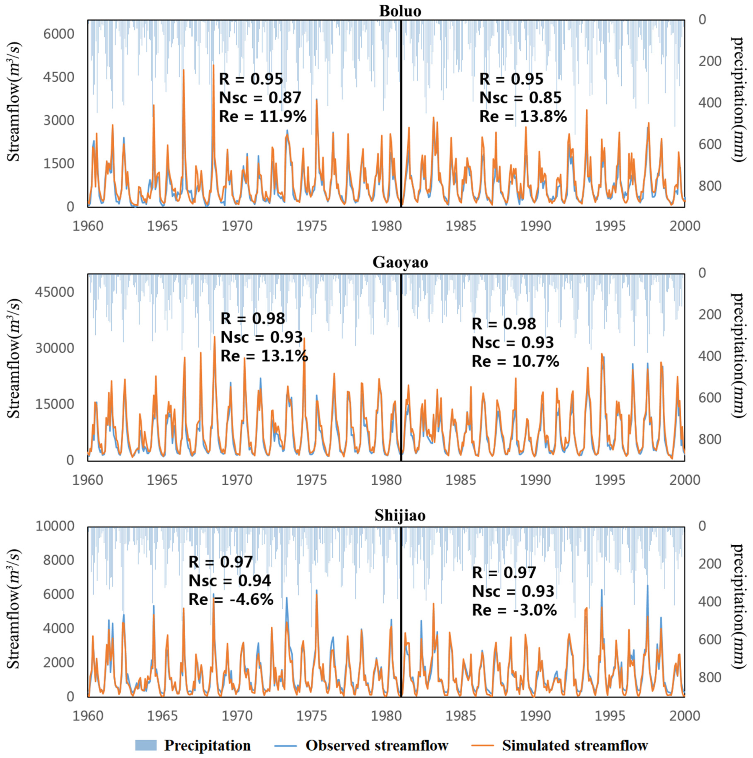
As shown in Figure 2, the monthly NSCEs of the three hydrological stations (Boluo, Gaoyao, and Shijiao) are all higher than 0.85 in both calibration (1960–1980) and validation (1981–2000) periods; all the correlation coefficients are higher than 0.95 with the absolute values of relative errors less than 15%. The results indicate that the VIC model performs satisfactorily for the hydrological simulation and maintains a reasonable water balance [25], demonstrating that the calibrated model can be used for the estimation of ETa in the PRB.

3.1.2. Annual ETa in the PRB

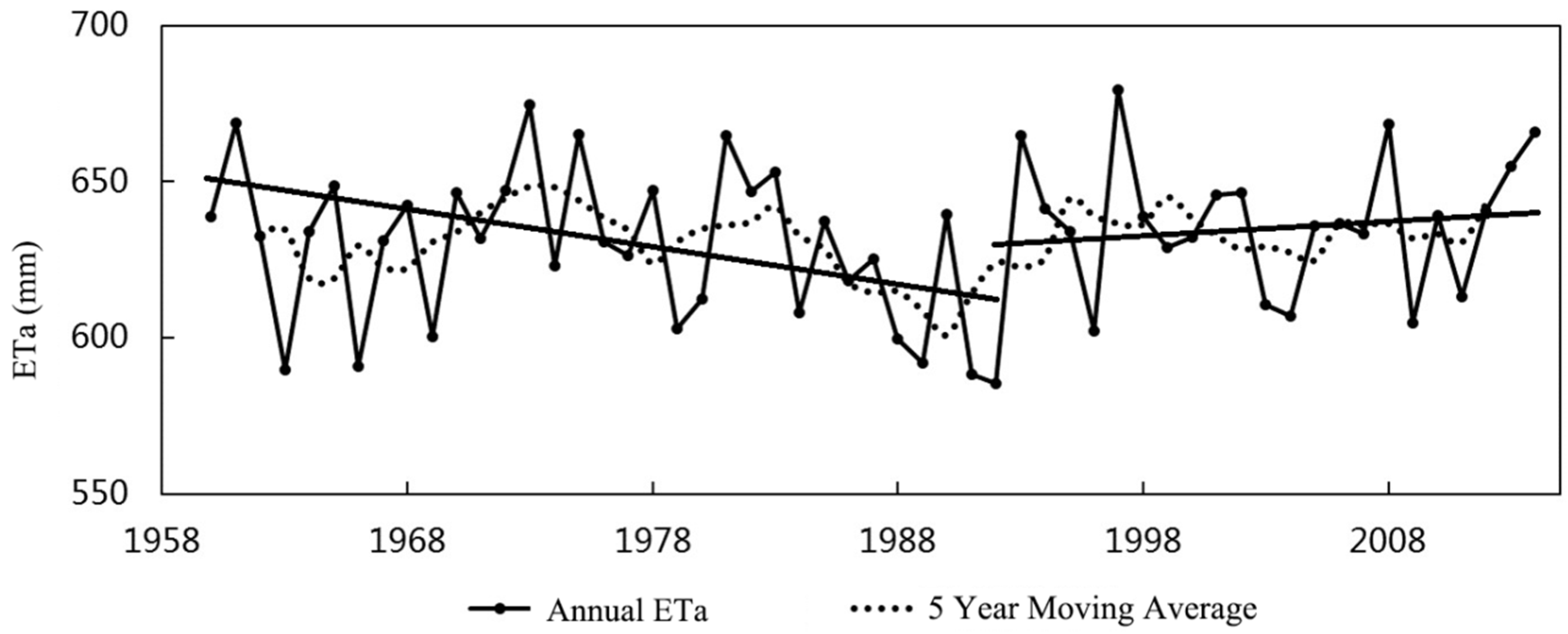
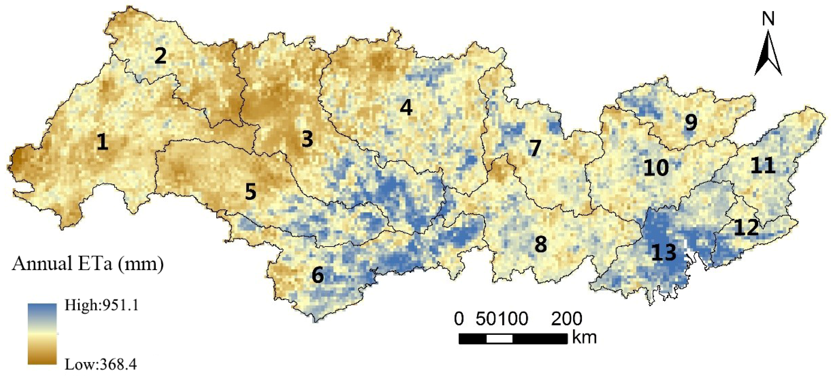
The daily ETa data of all grids in the entire basin exported by the VIC model from 1960 to 2014 were statistically analyzed at the spatial and temporal scales. From the statistical analyses, we obtained the annual sequence of the ETa over 55 years in the basin (Figure 3) and the spatial distribution of the annual average ETa (Figure 4).
The data shown in Figure 3 reveal that the annual average ETa in the PRB was 626.1 mm/a and varied from 585.5 to 679.3 mm over the 55 years. In terms of temporal changes, the annual ETa first decreased and then increased during the 55 years. Before the 1990s, the annual ETa generally showed a downward trend and reached the minimum value of 585.5mm in 1992. Subsequently, the annual ETa increased to a maximum value of 679.3 mm in 1997.
The prominent spatial heterogeneity in the spatial distribution of the ETa is displayed in Figure 4. The annual average ETa in the PRB was within the range of 368.4–951.1 mm. The high ETa values were mainly distributed around the estuary of the Pearl River Delta, and downstream of the Zuojiang, Youjiang, and Hongshui rivers as well. The low values mainly distributed in western region, including the sub-region of the Nanpan River, Beipan River, and the upper reaches of the Youjiang as well as Hongshui rivers.

3.1.3. Spatial-Temporal Variation of the ETa

The change trends of the ETa were analyzed by using the M–K trend test method at the monthly, seasonal, and yearly scales (Table 2 and Table 3). The results of the M–K test show that the M–K value of the annual ETa in the PRB during the period of 1960–2014 is 0.21, which means that the ETa generally showed a slight, but not significant increasing, trend over the past 55 years. The average change rate was approximately 0.042 mm/a, that is, it increased by about 2.34 mm in the past 55 years. At the seasonal scale, the ETa in the PRB showed a significant upward trend in summer (p < 0.05) and a significant downward trend in autumn (p < 0.01). At the monthly scale, the ETa across the whole basin significantly decreased in October (p < 0.1) and significantly increased in June (p < 0.05) and July (p < 0.01). Additionally, at the sub-region scale, the ETa in the upstream region displayed a more obvious downward trend, while the ETa in the downstream region exhibited a more obvious upward trend.
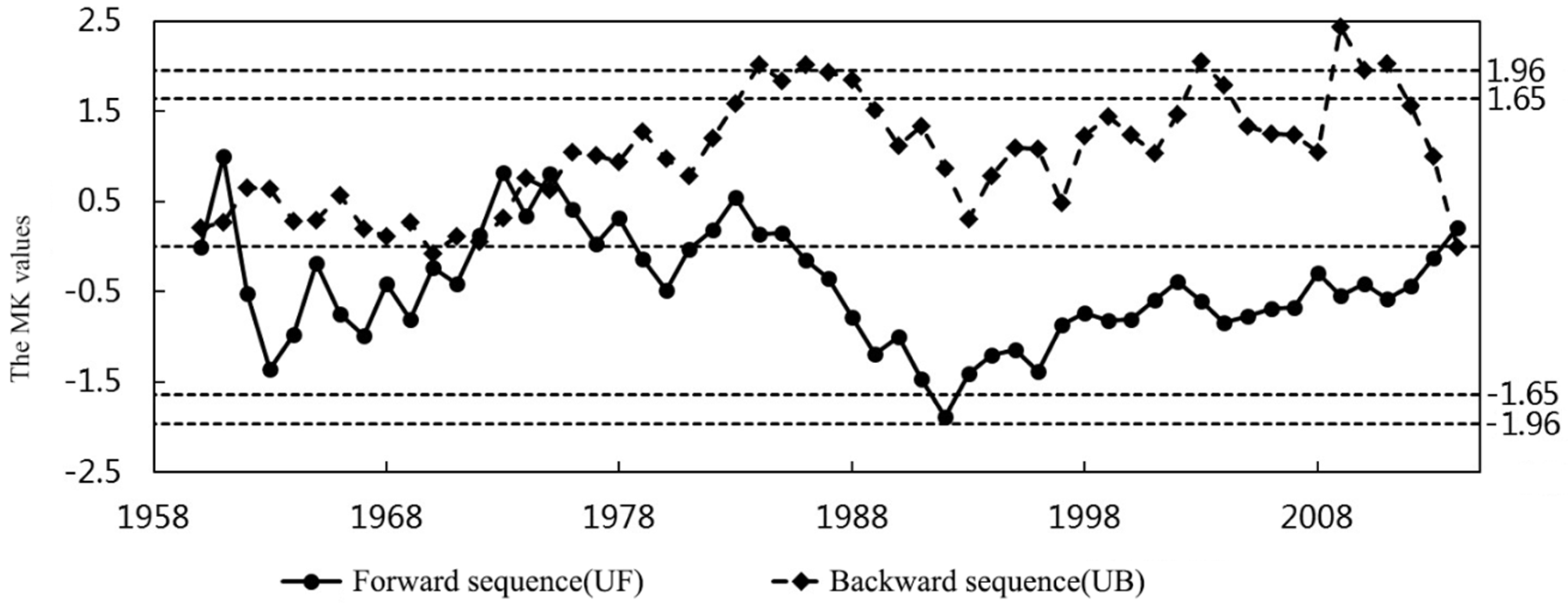
The data presented in Figure 5 reveal that the UF curve only comes in contact with the UB curve in 1973 and there was no significant intersection, which means that there is no obvious abrupt change over the 55 years in the PRB. According to the shape of the UF curve, the ETa roughly showed an obvious downward trend in the period of 1960–1992, with a M–K value of about −1.89 in the year 1992, passing the significant test at the 0.1 significance level (−1.65) and close to 0.05 significance level (−1.96). This means that from 1960 to 1992 the ETa had a decreasing trend in the PRB although there is no obvious abrupt change in the 55-year series; subsequently, the UF curve increased, indicating that the ETa in the basin gradually turned to an upward trend in the 1990s.
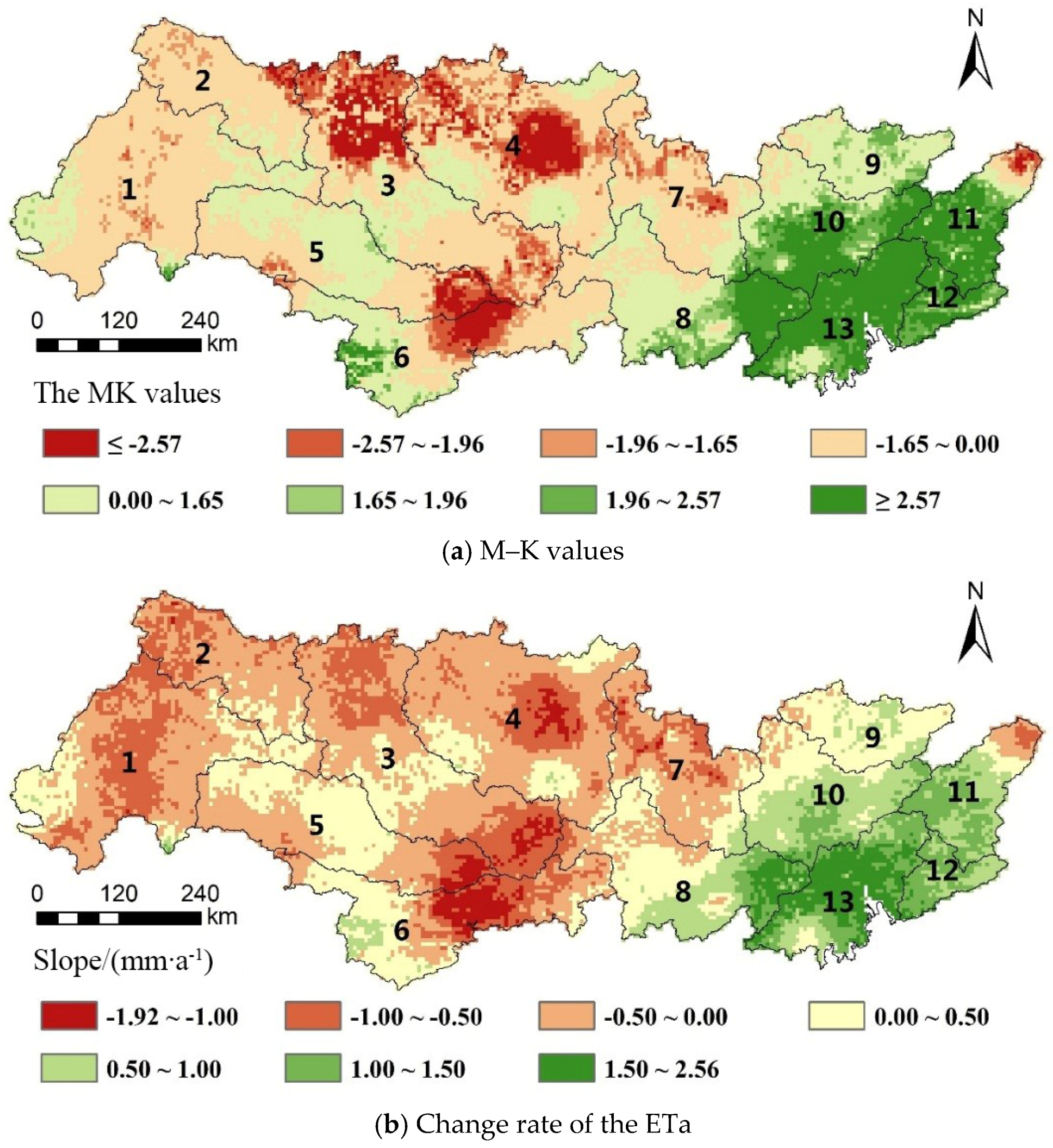
At the spatial scale (Figure 6a), the ETa in the upper stream of the PRB generally showed no significant increasing or decreasing trend. Some regions, including the sub-region of the Liujiang River, Zuojiang River and the upstream of the Hongshui River, exhibited a significant decreasing trend at the 0.05 significance level. Additionally, in the downstream region of the PRB, especially the Pearl River Delta, the Dongjiang River basin and the downstream of the Beijiang River, the ETa displayed a significant increasing trend at the 0.01 significance level. The change rate of the ETa in the PRB is shown in Figure 6b. The largest reduction of the ETa occurred in the south part of the PRB and the area with the largest increase was mainly located in the Pearl River Delta.

3.2. Relationships between the ETa and Climatic Factors

3.2.1. Partial Correlation Coefficient

In order to investigate the causes of the spatial distribution and temporal variation trend of the ETa in the PRB, a partial correlation coefficient analysis was conducted to evaluate the influence of various climatic factors on the ETa. With the aim of removing the interference of other factors as much as possible, ten climatic factors used in the relevant studies were selected to calculate the 9th order partial correlation coefficient of the ETa, and then we conducted a significance test by the Student’s test. The ten factors included: water quantity factors, such as precipitation (PREC), relative humidity (RH), water vapor pressure (VP); thermal factors, such as average temperature (TEMP), daily minimum and maximum temperature (TMIN, TMAX), daily temperature range (TMRG), sunshine hours (SH); dynamic factors, such as average pressure (PRESS), and mean wind speed (WIND). All the ten climatic factors are statistically independent from each other.
Accordingly, from the foregoing, we can learn that ETa in the PRB exhibited two different trends, namely before and after 1992. After analyzing the time series of climatic factors, we found their trends also changed around the year 1992. Thus, the ETa and climatic factors in the basin were divided into two periods (i.e., 1960–1992 and 1992–2014) for the convenience of calculation. The partial correlation coefficients of the influence of climatic factors on the ETa at different time scales in the two time periods are shown in Table 4.
During the 1960–1992 period, except for PREC, the VP and TEMP showed a significant correlation with the ETa both at the yearly scale, and the strong correlation of VP with ETa passed the significance test at the 0.01 level. At the monthly scale, the ETa showed significant correlations with the SH and PRESS. In addition, thermodynamic factors, such as WIND, TMAX, TMIN, and TMRG showed a high partial correlation with the ETa at the monthly scale in spring and summer.
During the 1992–2014 period, the SH had the most notable impact on the ETa (except for PREC), exhibiting a very significant correlation with a significant level of 0.01 in spring, summer and at the yearly scale. TEMP also had a very significant correlation with the ETa in spring, summer, and at the monthly and yearly scales. According to the data in Table 4, the partial correlation coefficients of the ETa and different climatic factors showed significant differences in the different time scales, which is consistent with the findings reported by Li et al. [44].

3.2.2. Temporal Variation of the Ten Climatic Factors

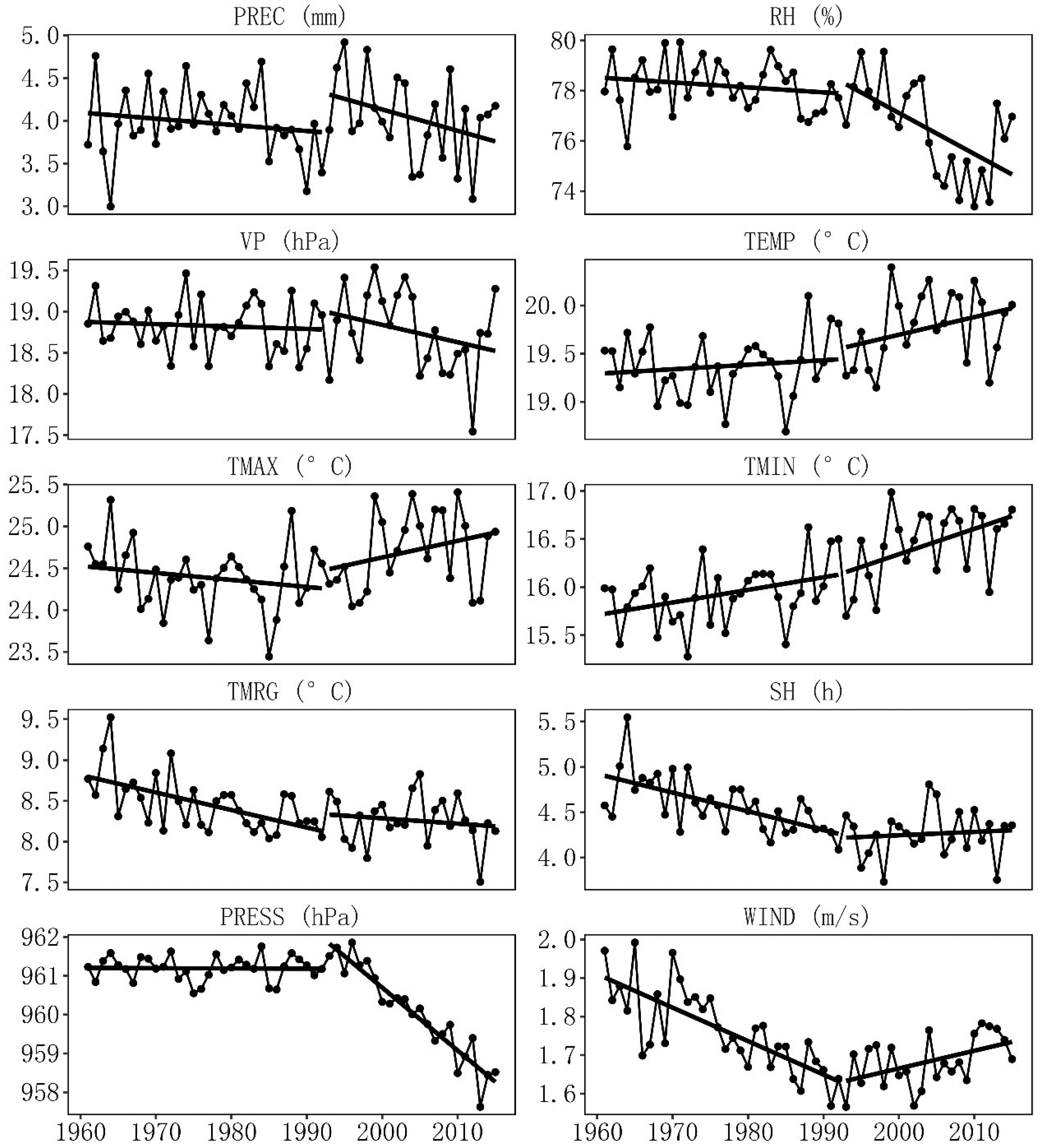
The change trends of the ten climatic factors in the PRB during the period of 1960–2014 are shown in Figure 7. The regression analysis results for each of the factors in the two periods of 1960–1992 and 1992–2014, revealed that factors including RH, TMAX, SH, PRESS, and WIND showed different change trends before and after 1992.
From 1960 to 1992, PREC, TEMP and VP, significantly correlated with the ETa at the yearly scale, but none showed obvious declining or rising trend. SH, which exhibited a very significant correlation with the ETa at the monthly scale, showed a significant declining trend. Thus, it can be speculated that the negative trend of the ETa in the PRB before 1992 may be mainly due to the significant decrease of SH. From 1992 to 2014, at the monthly and yearly scales, PRESS, TEMP, and SH showed significant correlations with the ETa. Compared with the period of 1960–1992, PRESS turned from a no apparent change trend to a significant decreasing trend; TEMP rose more significantly; SH turned from a significant decline to no obvious change trend, which indicate that the upward trend of the ETa in the PRB after 1992 may be due to the significant decrease of PRESS and the less sharp decline of SH.
In order to further investigate the main climatic factors affecting the ETa in each sub-region of the PRB, the partial correlation coefficients between the ETa and different climatic factors in each sub-region were calculated and analyzed at the yearly scale. The results, which are shown in Table 5, revealed that PREC is an important factor affecting the ETa in most regions. In addition, TEMP and VP had great influence on the ETa in the middle and lower reaches of the basin (i.e., in the sub-region of the Liujiang River, Zuojiang River, Yujiang River, Hegui River, etc.). Additionally, WIND also had a significant influence on the ETa in downstream areas, such as the Dongjiang River basin and the Pearl River Delta.

4. Discussion

4.1. Comparison with Related Studies

In the PRB, we found that the ETa showed a significant declining trend during the period of 1960–1992 and then gradually turns into an increasing trend from 1992 onwards. Zhang et al. stated the ETa decreased gradually from east to the west and our study showed a consistency with theirs. They also found decreasing wind speed and decreasing sunshine hours greatly dominated the change of actual evapotranspiration [75], which verified that sunshine duration is a dominant climatic factor of ETa in the PRB. However, only four climatic factors (i.e., temperature, precipitation, wind speed, and sunshine hours) and a shorter time series (1960–2005) were used in their study, causing a few differences with our study. Zhang and Chen found that the ETa in PRB showed an increasing trend during 2000–2014 [76], which is similar with the trend after the year 1992 in our study. However, Li et al. used the advection-aridity (A-A) model to carry out research in the PRB and their results were completely different from those of our study [77,78]. According to Li et al., the ETa in the PRB exhibited a significant decreasing trend from 1960 to 2008, which may be explained by the fact that the A-A model only considers a relatively ideal condition. In fact, according to the Penman–Monteith and Priestley–Taylor methods, the A-A model only roughly considers the vegetation and ignores the underlying surface details, which contributes to its possible low performance [79]. Thus, this indicates that the A-A model may not adequately reflect the actual situation and may be unsuitable for an extremely wet environment [80,81].
In addition, we also compared our results with the ones based on PE, ET0, and PET. Yao et al. found the annual PET in south China showed a decreasing trend then increased around 1995 [82]; Xing et al. also discovered the ET0 had a similar turning point in 1995 in Southeast China [40]. This change trend was also verified in Northwest China revealing that PE exhibited an obvious decreasing trend until early 1990s and such a downward trend reversed in 1993 [39]. A similar upward trend of land ET at the global scale was also confirmed by Zhang et al. during the period of 1981–2012 [14]. Their studies revealed that ET had an upward trend at the global scale and are also consistent to a certain extent with our results in the PRB during 1992–2014. Additionally, our study also shared similar characteristics with some studies on a national or global scale [7,14,33,38,39,83,84,85]. Based on the above relevant studies and our study, we could also speculate that the ET in the PRB experienced a turning point in the 1990s, in which it initially decreased and later ETa increased.
The trends of the seasonal ETa in the PRB had obvious regularity that exhibited a significant upward trend in summer and a decreasing trend in autumn. Zhang and Chen reported that the ETa increased in both summer and autumn, which is different from our study [76]. This inconsistency may be explained by the difference in the length of time series between the two studies. On the spatial scale, low ETa was mainly found in the western region with high elevation and lower vegetation coverage, while the eastern and central areas were characterized by high ETa. The results of our study showed that the spatial distribution of low ETa in the PRB was associated with elevation and vegetation types and coverage [76]. Notably, the ETa showed a significant increasing trend in the eastern region, and a decreasing trend in other regions, including the sub-region in the Liujiang River, Zuojiang River and the upstream of the Hongshui River, which showed significant spatial difference due to different topographic and climatic features.

4.2. The Dominant Climatic Factor of ETa in the PRB

In this study, ten climatic factors were chosen to examine their influence on the variation of the ETa in the PRB. According to the aforementioned analysis of the correlations between climatic factors and the ETa, SH can be regarded as the main factor influencing the variation of the ETa in the PRB. Since the decreasing SH had a significant correlation with the decreasing ETa during the period of 1960–1992, we were able to infer that SH was the major factor promoting the decrease of the ETa. The results are consistent with many former related studies [41,45,86,87,88]. For example, one study found that SH was the most important variable influencing PET in Southeast China [86]. Through the analysis of the contribution of various factors to ET0 variation, Wang et al. found that sunshine duration had the greatest impact on the variation of ET0 in coastal regions with increasing level of urbanization and large population, including the Southern China region [41] where the downstream areas of the PRB are located. Study in Guangdong Province, which belongs to the PRB, also determined that decreasing sunshine duration was the crucial climatic factor leading to the decreasing PE [87]. To some extent, the reliability of the findings in this study was reinforced by the above studies. Most previous studies concluded that the increasing cloud coverage and aerosol concentration would be the main causes of the decreasing sunlight [32,86,89]. It is widely known that, in recent decades, large amounts of aerosol were released to the atmosphere due to human activities, resulting in decreasing SH. Additionally, high-rise buildings in cities hinder the diffusion of aerosols more or less, thereby intensifying the decrease of SH. Thus, these may be the two reasons that SH was the dominant climatic factor influencing the ETa in the PRB, especially in the Pearl River Delta.
In terms of the previous analysis, we found that the partial correlation coefficients between the ETa and climatic factors showed significant differences in different time scales, which is consistent with the study of Li et al. [44]. Compared with the period of 1960–1992, PRESS turned into a significant decreasing trend; TEMP rose more clearly; SH turned from having a significantly declining trend to no obvious changing trend. Since PRESS had a negative correlation with the ETa [44], we also inferred that the increasing trend of the ETa in the PRB after 1992 may be due to the significant decrease of PRESS and the less sharp decline of SH. In addition, at the sub-regional scale, it is somewhat interesting that WIND had a significant correlation with the ETa in the downstream of the PRB including the Dongjiang River Basin and the Pearl River Delta. Considering the variation trend of WIND, we surmised that to a certain degree WIND may contribute to the variation of the ETa. Meanwhile, TEMP and VP had a great influence on the ETa in the middle and lower reaches of the basin. To explain these results, we reasoned that each region had its unique climatic and topographic condition, which resulted in the various correlated factors of ETa in different areas in the same period of time [44,76]. However, in general, it was indisputable that the variation of the ETa in the PRB was dominated by SH.
In particular, the variation of the ETa in the PRB is a complex process, due to the synthetical effects of related climatic factors. During the period of 1960–1992, even when the temperature rose slightly, the markedly decreasing SH led to the total decrease of the ETa. After 1992, with the more markedly rising temperature, SH decreased less sharply when PRESS fell steeply, ultimately resulting in the ETa turning into an upward trend.

4.3. Does the “Paradox” Exist When Using ETa Estimation?

According to the above analysis, over the past 55 years, the annual ETa showed a significant downward trend during the period of 1960–1992. However, the average temperature in the PRB showed an increasing trend during 1960–1992 (Figure 7) and then we can speculate that the “paradox” phenomenon existed in this period, i.e., the “paradox” phenomenon in the PRB can also be detected by using ETa estimation. Subsequently, the ETa gradually turned to an upward trend later in the 1992–2014 period. At the spatial scale, the ETa in the middle and upper stream of the PRB generally exhibited a non-significant decreasing trend when some of its parts showed a relatively significant decreasing trend. In the downstream areas, the ETa showed as a significant increasing trend. According to the above-mentioned results, in general, the “paradox” existed in the variation of ETa during the period of 1960–1992 in the middle-upper area of the PRB and the decline in SH mainly controlled the decrease in the ETa. Furthermore, an obvious decline of SH before the early 1990s in our study was associated with the “global dimming” and the recovery of SH after the 1990s roughly coincided with the “global brightening” [90], consistent with some previous studies [39,40]. The phenomenon of “global dimming and brightening” described by Wild et al. suggested that the declining global solar radiation during the period of 1960–1990s did not continue into the following years [90]. Some researchers concluded that cloud coverage and aerosol, which were in a way influenced by human activities, were the most likely factors to explain the “dimming and brightening”, and the strong aerosol effects of rising air pollution on the decline of solar radiation in China have also been confirmed [40,91]. These ideas could to some extent explain the “paradox” detected by ETa in the PRB, suggesting that we could use ETa to characterize the “evaporation paradox”.
Undoubtedly, the variation of the ETa resulted from synthetical effects of different climatic factors. Although temperature is always considered as a key driver of the ETa changes, it is neither the only factor nor the most decisive factor influencing the variation of the ETa in the PRB. In reality, each region has its own decisive factors. The so called “evaporation paradox” simply associated the ETa with temperature and neglected the effects of other related climatic factors and human activities, which may lead to increasing or decreasing ET. Therefore, to gain a deeper understanding of the “evaporation paradox”, further studies should fully consider the spatiotemporal variation of different influential factors, and focus on how their changes result in the spatiotemporal variations of ET.
Although this study analyzed the spatiotemporal variability of ETa and identified the dominant climatic factors and finally achieved some results, there are inevitably many remaining deficiencies. For example, as the VIC model was used to estimate the ETa and assess the impact of different climatic factors on ETa, the results will be more reliable if a sensitivity and uncertainty analysis are carried out [92,93]. The driving mechanism of climatic factors on ETa in the PRB is still unclear and needs further discussion. Hopefully, these deficiencies could be further discussed in the future in order to provide more information for understanding the advantages of the VIC model as well as more details of ETa in the PRB.

5. Conclusions

This study established a VIC model with a high spatial resolution of 0.05° in the PRB, and conducted a simulation of the ETa during the 1960–2014 period. The spatiotemporal variation of the simulated ETa and its influential climatic factors in recent decades were analyzed. The following conclusions can be drawn from the main results of this study:
(1)
The analysis of the simulated ETa derived from the VIC model showed that the mean annual ETa of the PRB was 626.1 mm. Additionally, overall, the annual ETa showed a slight but not significant increasing trend in the PRB over the past 55 years, whereas it showed a negative trend during the 1960–1992 period. At the spatial scale, the ETa in the middle and upper stream of the PRB generally exhibited a non-significant decreasing trend, except for some parts which showed a relatively significant decreasing trend. In the downstream areas, especially in the Pearl River Delta and Dongjiang River Basin, the ETa exhibited a significant increasing trend.
(2)
According to the analysis of the partial correlation coefficients, the partial correlation coefficients between the ETa and climatic factors varied at different time scales. From 1960 to 1992, the ETa in the PRB had significant correlations with TEMP and VP at the yearly scale. Additionally, it also significantly correlated with SH and PRESS at the monthly scale. From 1992 to 2014, it had a significant correlation with TEMP, SH, and PRESS. In general, after considering the variations of these factors, the changes of the ETa across the PRB were mainly influenced by SH and PRESS.
(3)
Overall, mainly due to the decreasing SH, the “paradox” phenomenon existed in the middle-upper area of the PRB during the period of 1960–1992. The phenomenon could be explained by the “global dimming” event in China, resulting from the changes of cloud coverage and aerosol accumulation. The “paradox” phenomenon in the PRB can be detected by ETa estimation, which implies we could also use ETa to further verify the “evaporation paradox”.

Author Contributions

Z.W. conceived and designed the research; W.G. performed the data analysis and wrote the manuscript; G.H. proposed some constructive suggestions about the research.

Funding

This research was funded by the National Key R and D Program of China (2018YFC1508200), and the National Natural Science Foundation of China (grant Nos. 51879107, 51709117).

Acknowledgments

We have the pleasure to extend our cordial gratitude to Guest Editor Sébastien Garrigues, Assistant Editor Xue Liang, and two anonymous reviewers for their insightful review and professional revision suggestions, which are greatly helpful for further improvement of this manuscript.

Conflicts of Interest

The authors declare no conflict of interest.

References

  1. Falamarzi, Y.; Palizdan, N.; Huang, Y.F.; Lee, T.S. Estimating evapotranspiration from temperature and wind speed data using artificial and wavelet neural networks (WNNs). Agric. Water Manage. 2014, 140, 26–36. [Google Scholar] [CrossRef]
  2. Fisher, J.; Melton, F.; Middleton, E.; Hain, C.; Anderson, M.; Allen, R.; McCabe, M.; Hook, S.; Baldocchi, D.; Townsend, P.; et al. The future of evapotranspiration: Global requirements for ecosystem functioning, carbon and climate feedbacks, agricultural management, and water resources. Water Resour. Res. 2017, 53, 2618–2626. [Google Scholar] [CrossRef]
  3. Katul, G.G.; Oren, R.; Manzoni, S.; Higgins, C.; Parlange, M.B. Evapotranspiration: A process driving mass transport and energy exchange in the soil-plant-atmosphere-climate system. Rev. Geophys. 2012, 7. [Google Scholar] [CrossRef]
  4. Mu, Q.; Zhao, M.; Running, S.W. Improvements to a MODIS global terrestrial evapotranspiration algorithm. Remote Sens. Environ. 2011, 115, 1781–1800. [Google Scholar] [CrossRef]
  5. Trenberth, K.E.; Fasullo, J.T.; Kiehl, J. Earth’s Global Energy Budget. Bull. Am. Meteorol. Soc. 2009, 90, 311–324. [Google Scholar] [CrossRef]
  6. Wang, K.; Dickinson, R.E. A review of global terrestrial evapotranspiration: Observation, modeling, climatology, and climatic variability. Rev. Geophys. 2012, 50. [Google Scholar] [CrossRef]
  7. Peterson, T.C.; Golubev, V.S.; Groisman, P.Y. Evaporation losing its strength. Nature 1995, 377, 687–688. [Google Scholar] [CrossRef]
  8. Kool, D.; Agam, N.; Lazarovitch, N.; Heitman, J.L.; Sauer, T.J.; Ben-Gal, A. A review of approaches for evapotranspiration partitioning. Agric. For. Meteorol. 2014, 184, 56–70. [Google Scholar] [CrossRef]
  9. Cammalleri, C.; Agnese, C.; Ciraolo, G.; Minacapilli, M.; Provenzano, G.; Rallo, G. Actual evapotranspiration assessment by means of a coupled energy/hydrologic balance model: Validation over an olive grove by means of scintillometry and measurements of soil water contents. J. Hydrol. 2010, 392, 70–82. [Google Scholar] [CrossRef]
  10. Xu, C.-Y.; Singh, V.P. Evaluation of three complementary relationship evapotranspiration models by water balance approach to estimate actual regional evapotranspiration in different climatic regions. J. Hydrol. 2005, 308, 105–121. [Google Scholar] [CrossRef]
  11. Wang, Z.; Li, J.; Lai, C.; Wang, R.Y.; Chen, X.; Lian, Y. Drying tendency dominating the global grain production area. Global Food Secur. 2018, 16, 138–149. [Google Scholar] [CrossRef]
  12. Zhong, R.; Chen, X.; Lai, C.; Wang, Z.; Lian, Y.; Yu, H.; Wu, X. Drought monitoring utility of satellite-based precipitation products across mainland China. J. Hydrol. 2019, 568, 343–359. [Google Scholar] [CrossRef]
  13. Li, J.; Wang, Z.; Lai, C.; Wu, X.; Zeng, Z.; Chen, X.; Lian, Y. Response of net primary production to land use and land cover change in mainland China since the late 1980s. Sci. Total Environ. 2018, 639, 237–247. [Google Scholar] [CrossRef] [PubMed]
  14. Zhang, Y.; Peña-Arancibia, J.L.; McVicar, T.R.; Chiew, F.H.S.; Vaze, J.; Liu, C.; Lu, X.; Zheng, H.; Wang, Y.; Liu, Y.Y.; et al. Multi-decadal trends in global terrestrial evapotranspiration and its components. Sci. Rep. 2016, 6, 19124. [Google Scholar] [CrossRef] [PubMed] [Green Version]
  15. Allen, R.G.; Pereira, L.S.; Howell, T.A.; Jensen, M.E. Evapotranspiration information reporting: I. Factors governing measurement accuracy. Agric. Water Manage. 2011, 98, 899–920. [Google Scholar] [CrossRef] [Green Version]
  16. Allen, R.G.; Pereira, L.S.; Raes, D. Crop Evapotranspiration: Guidelines for Computing Crop Requirements; Irrigation and Drainage Paper No. 56; FAO: Rome, Italy, 1998; p. 300. [Google Scholar]
  17. Thornthwaite, C.W. An Approach toward a Rational Classification of Climate. Geogr. Rev. 1948, 38, 55–94. [Google Scholar] [CrossRef]
  18. Penman, H.L. Natural evaporation from open water, bare soil and grass. Proc. R. Soc. Lond. Ser. A Math. Phys. Sci. 1948, 193, 120–145. [Google Scholar] [Green Version]
  19. Fan, L.; Zhang, G. Relationship between Actual Evapotranspiration and Potential Evapotranspiration in Guangdong. J. Guangdong Ocean Univ. 2013, 33, 71–77. (In Chinese) [Google Scholar]
  20. McMahon, T.A.; Peel, M.C.; Lowe, L.; Srikanthan, R.; McVicar, T.R. Estimating actual, potential, reference crop and pan evaporation using standard meteorological data: A pragmatic synthesis. Hydrol. Earth Syst. Sci. 2013, 17, 1331–1363. [Google Scholar] [CrossRef]
  21. Gao, G.; Chen, D.; Xu, C.; Simelton, E. Trend of estimated actual evapotranspiration over China during 1960–2002. J. Geophys. Res. 2007, 112, D11120. [Google Scholar] [CrossRef]
  22. Cao, G.; Han, D.; Song, X. Evaluating actual evapotranspiration and impacts of groundwater storage change in the North China Plain. Hydrol. Processes. 2014, 28, 1797–1808. [Google Scholar] [CrossRef]
  23. Larsen, M.A.D.; Christensen, J.H.; Drews, M.; Butts, M.B.; Refsgaard, J.C. Local control on precipitation in a fully coupled climate-hydrology model. Sci. Rep. 2016, 6, 22927. [Google Scholar] [CrossRef] [PubMed] [Green Version]
  24. Xie, Z.; Yuan, F.; Duan, Q.; Zheng, J.; Liang, M.; Chen, F. Regional Parameter Estimation of the VIC Land Surface Model: Methodology and Application to River Basins in China. J. Hydrometeor. 2007, 8, 447–468. [Google Scholar] [CrossRef] [Green Version]
  25. Wang, Z.; Zhong, R.; Lai, C.; Zeng, Z.; Lian, Y.; Bai, X. Climate change enhances the severity and variability of drought in the Pearl River Basin in South China in the 21st century. Agric. For. Meteorol. 2018, 249, 149–162. [Google Scholar] [CrossRef]
  26. Yan, D.; Werners, S.E.; Ludwig, F.; Huang, H.Q. Hydrological response to climate change: The Pearl River, China under different RCP scenarios. J. Hydrol. Reg. Stud. 2015, 4, 228–245. [Google Scholar] [CrossRef] [Green Version]
  27. Wu, C.; Huang, G.; Yu, H.; Chen, Z.; Ma, J. Impact of Climate Change on Reservoir Flood Control in the Upstream Area of the Beijiang River Basin, South China. J. Hydrometeor. 2014, 15, 2203–2218. [Google Scholar] [CrossRef]
  28. Shah, H.L.; Mishra, V. Hydrologic Changes in Indian Subcontinental River Basins (1901–2012). J. Hydrometeor. 2016, 17, 2667–2687. [Google Scholar] [CrossRef]
  29. Liu, M.; Adam, J.C.; Hamlet, A.F. Spatial-temporal variations of evapotranspiration and runoff/precipitation ratios responding to the changing climate in the Pacific Northwest during 1921–2006. J. Geophys. Res. Atmos. 2013, 118, 380–394. [Google Scholar] [CrossRef]
  30. Bohn, T.J.; Vivoni, E.R. Process-based characterization of evapotranspiration sources over the North American monsoon region. Water Resour. Res. 2016, 52, 358–384. [Google Scholar] [CrossRef]
  31. Trenberth, K.E.; Dai, A.G.; van der Schrier, G.; Jones, P.D.; Barichivich, J.; Briffa, K.R.; Sheffield, J. Global warming and changes in drought. Nat. Clim. Change. 2014, 4, 17–22. [Google Scholar] [CrossRef]
  32. Roderick, M.L.; Farquhar, G.D. The cause of decreased pan evaporation over the past 50 years. Science 2002, 298, 1410–1411. [Google Scholar] [PubMed]
  33. Cong, Z.T.; Yang, D.W.; Ni, G.H. Does evaporation paradox exist in China? Hydrol. Earth Syst. Sci. 2009, 13, 357–366. [Google Scholar] [CrossRef] [Green Version]
  34. Jung, M.; Reichstein, M.; Ciais, P.; Seneviratne, S.I.; Sheffield, J.; Goulden, M.L.; Bonan, G.; Cescatti, A.; Chen, J.; de Jeu, R.; et al. Recent decline in the global land evapotranspiration trend due to limited moisture supply. Nature 2010, 467, 951. [Google Scholar] [CrossRef] [PubMed]
  35. Hobbins, M.T.; Ramírez, J.A.; Brown, T.C. Trends in pan evaporation and actual evapotranspiration across the conterminous U.S.: Paradoxical or complementary? Geophys. Res. Lett. 2004, 31. [Google Scholar] [CrossRef] [Green Version]
  36. Liu, B.; Xu, M.; Henderson, M.; Gong, W. A spatial analysis of pan evaporation trends in China, 1955–2000. J. Geophys. Res. Atmos. 2004, 109, D15102–D15109. [Google Scholar] [CrossRef]
  37. Zhang, Q.; Qi, T.; Li, J.; Singh, V.P.; Wang, Z. Spatiotemporal variations of pan evaporation in China during 1960–2005: Changing patterns and causes. Int. J. Climatol. 2015, 35, 903–912. [Google Scholar] [CrossRef]
  38. Thomas, A. Spatial and temporal characteristics of potential evapotranspiration trends over China. Int. J. Climatol. 2000, 20, 381–396. [Google Scholar] [CrossRef]
  39. Li, Z.; Chen, Y.; Shen, Y.; Liu, Y.; Zhang, S. Analysis of changing pan evaporation in the arid region of Northwest China. Water Resour. Res. 2013, 49, 2205–2212. [Google Scholar] [CrossRef]
  40. Xing, W.; Wang, W.; Shao, Q.; Yu, Z.; Yang, T.; Fu, J. Periodic fluctuation of reference evapotranspiration during the past five decades: Does Evaporation Paradox really exist in China? Sci. Rep. 2016, 6, 39503. [Google Scholar] [CrossRef]
  41. Wang, Z.; Xie, P.; Lai, C.; Chen, X.; Wu, X.; Zeng, Z.; Li, J. Spatiotemporal variability of reference evapotranspiration and contributing climatic factors in China during 1961–2013. J. Hydrol. 2017, 544, 97–108. [Google Scholar] [CrossRef]
  42. Ukkola, A.M.; Prentice, I.C. A worldwide analysis of trends in water-balance evapotranspiration. Hydrol. Earth Syst. Sci. 2013, 17, 4177–4187. [Google Scholar] [CrossRef] [Green Version]
  43. Duethmann, D.; Bloschl, G. Why has catchment evaporation increased in the past 40 years? A data-based study in Austria. Hydrol. Earth Syst. Sci. 2018, 22, 5143. [Google Scholar] [CrossRef]
  44. Li, X.; Gemmer, M.; Zhai, J.; Liu, X.; Su, B.; Wang, Y. Spatio-temporal variation of actual evapotranspiration in the Haihe River Basin of the past 50 years. Quat. Int. 2013, 304, 133–141. [Google Scholar] [CrossRef]
  45. Wang, Y.; Liu, B.; Su, B.; Zhai, J.; Gemmer, M. Trends of Calculated and Simulated Actual Evaporation in the Yangtze River Basin. J. Clim. 2011, 24, 4494–4507. [Google Scholar] [CrossRef]
  46. Matin, M.A.; Bourque, C.P.-A. Assessing spatiotemporal variation in actual evapotranspiration for semi-arid watersheds in northwest China: Evaluation of two complementary-based methods. J. Hydrol. 2013, 486, 455–465. [Google Scholar] [CrossRef]
  47. Zhu, G.; Su, Y.; Li, X.; Zhang, K.; Li, C. Estimating actual evapotranspiration from an alpine grassland on Qinghai-Tibetan plateau using a two-source model and parameter uncertainty analysis by Bayesian approach. J. Hydrol. 2013, 476, 42–51. [Google Scholar] [CrossRef]
  48. Wu, J.; Chen, X. Spatiotemporal trends of dryness/wetness duration and severity: The respective contribution of precipitation and temperature. Atmos. Res. 2019, 216, 176–185. [Google Scholar] [CrossRef]
  49. Wang, Z.; Qin, J.; Chen, X. Variation characteristics and impact factors of pan evaporation in Pearl River Basin, China. Trans. Chin. Soc. Agric. Eng. 2010, 26, 73–77. (In Chinese) [Google Scholar]
  50. Lai, C.; Zhong, R.; Wang, Z.; Wu, X.; Chen, X.; Wang, P.; Lian, Y. Monitoring hydrological drought using long-term satellite-based precipitation data. Sci. Total Environ. 2019, 649, 1198–1208. [Google Scholar] [CrossRef]
  51. Wang, Z.; Lai, C.; Chen, X.; Yang, B.; Zhao, S.; Bai, X. Flood hazard risk assessment model based on random forest. J. Hydrol. 2015, 527, 1130–1141. [Google Scholar] [CrossRef]
  52. Zhou, Y.; Lai, C.; Wang, Z.; Chen, X.; Zeng, Z.; Chen, J.; Bai, X. Quantitative Evaluation of the Impact of Climate Change and Human Activity on Runoff Change in the Dongjiang River Basin, China. Water 2018, 10, 571. [Google Scholar] [CrossRef]
  53. Wu, X.; Wang, Z.; Guo, S.; Liao, W.; Zeng, Z.; Chen, X. Scenario-based projections of future urban inundation within a coupled hydrodynamic model framework: A case study in Dongguan City, China. J. Hydrol. 2017, 547, 428–442. [Google Scholar] [CrossRef]
  54. Lai, C.; Chen, X.; Wang, Z.; Wu, X.; Zhao, S.; Wu, X.; Bai, W. Spatio-temporal variation in rainfall erosivity during 1960–2012 in the Pearl River Basin, China. CATENA 2016, 137, 382–391. [Google Scholar] [CrossRef]
  55. Liu, B.; Peng, S.; Liao, Y.; Long, W. The causes and impacts of water resources crises in the Pearl River Delta. J. Cleaner Prod. 2018, 177, 413–425. [Google Scholar] [CrossRef]
  56. Wang, Z.; Li, J.; Lai, C.; Zeng, Z.; Zhong, R.; Chen, X.; Zhou, X.; Wang, M. Does drought in China show a significant decreasing trend from 1961 to 2009? Sci. Total Environ. 2017, 579, 314–324. [Google Scholar] [CrossRef] [PubMed]
  57. FAO; IIASA; ISRIC; ISSCAS; JRC. Harmonized World Soil Database (Version 1.2); FAO: Rome, Italy, 2012. [Google Scholar]
  58. Saxton, K.E.; Rawls, W.J. Soil water characteristic estimates by texture and organic matter for hydrologic solutions. Soil Sci. Soc. Am. J. 2006, 70, 1569–1578. [Google Scholar] [CrossRef]
  59. Hansen, M.; Defries, R.; Townshend, J.; Sohlberg, R. Global land cover classification at 1 km spatial resolution using a classification tree approach. Int. J. Remote Sens. 2000, 21, 1331–1364. [Google Scholar] [CrossRef]
  60. Shafer, M.A.; Fiebrich, C.A.; Arndt, D.S.; Fredrickson, S.E.; Hughes, T.W. Quality assurance procedures in the Oklahoma Mesonetwork. J. Atmos. Oceanic Technol. 2000, 17, 474–494. [Google Scholar] [CrossRef]
  61. Estevez, J.; Garcia-Marin, A.P.; Morabito, J.A.; Cavagnaro, M. Quality assurance procedures for validating meteorological input variables of reference evapotranspiration in mendoza province (Argentina). Agric. Water Manage. 2016, 17, 96–109. [Google Scholar] [CrossRef]
  62. Lohmann, D.; Raschke, E.; Nijssen, B.; Lettenmaier, D.P. Regional scale hydrology: I. Formulation of the VIC-2L model coupled to a routing model. Hydrol. Sci. J. 1998, 43, 131–141. [Google Scholar] [CrossRef]
  63. Liang, X.; Lettenmaier, D.P.; Wood, E.F.; Burges, S.J. A simple hydrologically based model of land surface water and energy fluxes for general circulation models. J. Geophys. Res. Atmos. 1994, 99, 14415–14428. [Google Scholar] [CrossRef]
  64. Martínez-Lozano, J.A.; Tena, F.; Onrubia, J.E.; De La Rubia, J. The historical evolution of the Ångström formula and its modifications: Review and bibliography. Agric. For. Meteorol. 1984, 33, 109–128. [Google Scholar] [CrossRef]
  65. Mann, H.B. Nonparametric tests against trend. Econometrica 1945, 13, 245–259. [Google Scholar] [CrossRef]
  66. Kendall, M.G. Rank Correlation Methods, 4th ed.; Griffin: London, UK, 1975; pp. 1–200. [Google Scholar]
  67. Yang, H.; Yang, D.; Hu, Q.; Lv, H. Spatial variability of the trends in climatic variables across China during 1961–2010. Theor. Appl. Climatol. 2015, 120, 773–783. [Google Scholar] [CrossRef]
  68. Yue, S.; Wang, C.Y. Applicability of prewhitening to eliminate the influence of serial correlation on the Mann-Kendall test. Water Resour. Res. 2002, 38, 41–47. [Google Scholar] [CrossRef]
  69. Jones, J.R.; Schwartz, J.S.; Ellis, K.N.; Hathaway, J.M.; Jawdy, C.M. Temporal variability of precipitation in the Upper Tennessee Valley. J. Hydrol. Reg. Stud. 2015, 3, 125–138. [Google Scholar] [CrossRef] [Green Version]
  70. Pearson, K. On some novel properties of partial and multiple correlation coefficients in a universe of manifold characteristics. Biometrika 1916, 11, 231–238. [Google Scholar] [CrossRef]
  71. Yule, G.U.; Kendall, M.G. An Introduction to the Theory of Statistics, 14th ed.; Charles Griffin & Co.: Belmont, CA, USA, 1965. [Google Scholar]
  72. Jukić, D.; Denić-Jukić, V. Investigating relationships between rainfall and karst-spring discharge by higher-order partial correlation functions. J. Hydrol. 2015, 530, 24–36. [Google Scholar] [CrossRef]
  73. Fan, Y.; Chen, Y.; Liu, Y.; Li, W. Variation of baseflows in the headstreams of the Tarim River Basin during 1960–2007. J. Hydrol. 2013, 487, 98–108. [Google Scholar] [CrossRef]
  74. Schafer, J.; Opgenrhein, R.; Zuber, V.; Ahdesmaki, M.; Silva, A.P.D.; Strimmer, A.K. Corpcor: Efficient Estimation of Covariance and (Partial) Correlation. 2015. Available online: https://rdrr.io/cran/corpcor/ (accessed on 9 May 2019).
  75. Zhang, Q.; Xu, C.-Y.; Chen, Y.D.; Ren, L. Comparison of evapotranspiration variations between the Yellow River and Pearl River basin, China. Stochastic Environ. Res. Risk Assess. 2011, 25, 139–150. [Google Scholar] [CrossRef]
  76. Zhang, T.; Chen, Y. Analysis of Dynamic Spatiotemporal Changes in Actual Evapotranspiration and Its Associated Factors in the Pearl River Basin Based on MOD16. Water 2017, 9, 832. [Google Scholar] [CrossRef]
  77. Wu, P.; Li, X.C.; Jiang, T.; Wen, S.S.; Wang, Y.J.; Qiu, X.F. Spatio-temporal variation of actual evapotranspiration and its impact factors in the Pearl River Basin, China. J. Trop. Meteorol. 2017, 23. (In Chinese) [Google Scholar] [CrossRef]
  78. Brutsaert, W.; Stricker, H. An advection-aridity approach to estimate actual regional evapotranspiration. Water Resour. Res. 1979, 15, 443–450. [Google Scholar] [CrossRef]
  79. Ershadi, A.; McCabe, M.F.; Evans, J.P.; Chaney, N.W.; Wood, E.F. Multi-site evaluation of terrestrial evaporation models using FLUXNET data. Agric. For. Meteorol. 2014, 187, 46–61. [Google Scholar] [CrossRef]
  80. Qualls, R.J.; Gultekin, H. Influence of components of the advection-aridity approach on evapotranspiration estimation. J. Hydrol. 1997, 199, 3–12. [Google Scholar] [CrossRef]
  81. Han, S.; Hu, H.; Tian, F. Evaluation of applicability of three evapotranspiration models using meteorological data. J. Hydraul. Eng. 2009, 40, 75–81. (In Chinese) [Google Scholar]
  82. Yao, Y.; Zhao, S.; Zhang, Y.; Jia, K.; Liu, M. Spatial and decadal variations in potential evapotranspiration of China based on reanalysis datasets during 1982–2010. Atmosphere 2014, 5, 737–754. [Google Scholar] [CrossRef]
  83. Zhang, D.; Liu, X.; Hong, H. Assessing the effect of climate change on reference evapotranspiration in China. Stochastic Environ. Res. Risk Assess. 2013, 27, 1871–1881. [Google Scholar] [CrossRef]
  84. Zhang, K.; Kimball, J.S.; Nemani, R.R.; Running, S.W.; Hong, Y.; Gourley, J.J.; Yu, Z. Vegetation Greening and Climate Change Promote Multidecadal Rises of Global Land Evapotranspiration. Sci. Rep. 2015, 5, 15956. [Google Scholar] [CrossRef]
  85. Huang, H.; Han, Y.; Cao, M.; Song, J.; Xiao, H.; Cheng, W. Spatiotemporal Characteristics of Evapotranspiration Paradox and Impact Factors in China in the Period of 1960–2013. Adv. Meteorol. 2015, 2015, 1–10. [Google Scholar] [CrossRef]
  86. Yin, Y.; Wu, S.; Chen, G.; Dai, E. Attribution analyses of potential evapotranspiration changes in China since the 1960s. Theor. Appl. Climatol. 2010, 101, 19–28. [Google Scholar] [CrossRef]
  87. He, Y.; Lin, K.; Chen, X.; Ye, C.; Cheng, L. Classification-Based Spatiotemporal Variations of Pan Evaporation Across the Guangdong Province, South China. Water Resour. Manage. 2015, 29, 901–912. [Google Scholar] [CrossRef]
  88. Wu, X.; Guo, S.; Yin, J.; Yang, G.; Zhong, Y.; Liu, D. On the event-based extreme precipitation across China: Time distribution patterns, trends, and return levels. J. Hydrol. 2018, 562, 305–317. [Google Scholar] [CrossRef]
  89. Zhang, Q.; Xu, C.-Y.; Chen, X. Reference evapotranspiration changes in China: Natural processes or human influences? Theor. Appl. Climatol. 2011, 103, 479–488. [Google Scholar] [CrossRef]
  90. Wild, M.; Gilgen, H.; Roesch, A.; Ohmura, A.; Long, C.N.; Dutton, E.G.; Forgan, B.; Kallis, A.; Russak, V.; Tsvetkov, A. From Dimming to Brightening: Decadal Changes in Solar Radiation at Earth’s Surface. Science 2005, 308, 847–850. [Google Scholar] [CrossRef] [PubMed]
  91. She, D.; Xia, J.; Zhang, Y. Changes in reference evapotranspiration and its driving factors in the middle reaches of Yellow River Basin, China. Sci. Total Environ 2017, 607–608, 1151–1162. [Google Scholar] [CrossRef]
  92. Camillo, P.J.; Gurney, R.J. A sensitivity analysis of a numerical model for estimating evapotranspiration. Water Resour. Res. 1984, 20, 105–112. [Google Scholar] [CrossRef]
  93. Coleman, G.; DeCoursey, D.G. Sensitivity and model variance analysis applied to some evaporation and evapotranspiration models. Water Resour. Res. 1976, 12, 873–879. [Google Scholar] [CrossRef]
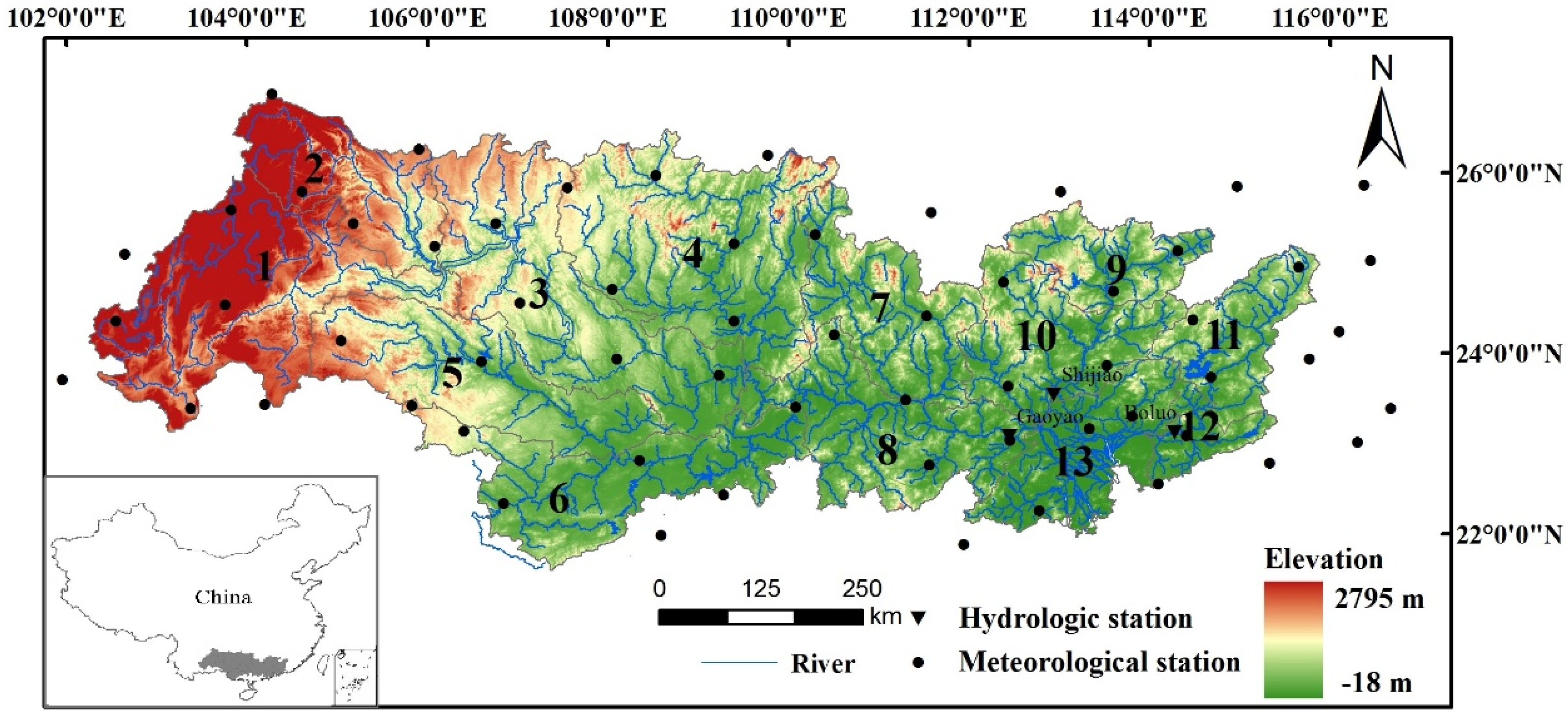
Figure 1. General location of the Pearl River Basin and the sub-regions. Notes: 1: Nanpan River; 2: Beipan River; 3: Hongshui River; 4: Liujiang River; 5: Youjiang River; 6: Zuojiang River and the main stream of the Yujiang River; 7: Hegui River; 8: Qianxun River and Xijiang River; 9: Upstream of the Dakengkou sub-region in the Beijiang River; 10: Downstream of the Dakengkou sub-region in the Beijiang River; 11: Upstream of the Qiujiangkou sub-region in the Dongjiang River; 12: Downstream of the Qiujiangkou sub-region in the Dongjiang River; 13: Pearl River Delta.
Atmosphere 10 00340 g001
Figure 2. Calibration and validation results of the VIC model.
Atmosphere 10 00340 g002
Figure 3. Annual ETa of the Pearl River Basin during 1960–2014 (α = 0.05).
Atmosphere 10 00340 g003
Figure 4. Distribution of the annual average ETa in the Pearl River Basin during 1960–2014. The name of the sub-regions refer to those in Figure 1.
Atmosphere 10 00340 g004
Figure 5. The M–K test results of the annual ETa during 1960–2014 in the Pearl River Basin. UF represents the statistics of forward sequence, UB the statistics of backward sequence.
Atmosphere 10 00340 g005
Figure 6. Spatial distribution of the trends of the annual ETa identified by the M–K test. (a) M–K values; (b) Change rate of the ETa. The name of the sub-regions refers to those in Figure 1.
Atmosphere 10 00340 g006
Figure 7. Variation trends (α = 0.05) of the ten climatic factors in the Pearl River Basin.
Atmosphere 10 00340 g007
Table 1. Meteorological and hydrological data used in this study.
Data CategoryData TypeSourceUnit
MeteorologicalPrecipitationThe Chinese Meteorological Administrationmm
Max daily air temperature°C
Min daily air temperature°C
Wind speedm/s
Sunshine hoursh
Shortwave radiationW/m2
Relative humidity%
HydrologicalObserved streamflowHydrological stationsm3/s
Table 2. M–K values for the ETa in the Pearl River Basin and its sub-regions at the monthly scale.
RegionJanuaryFebruaryMarchAprilMayJuneJulyAugustSeptemberOctoberNovember December
10.250.430.41−0.180.570.820.01−0.72−1.6−1.81△−1.74△−1.95△
2−1.440.310.52−0.83−0.241.21.33−0.73−1.43−1.47−1.36−2.45▲
3−1.60.850.7−1.87△−0.381.75△0.57−1.69△−0.91−1.63−1.71△−1.34
4−1.81△0.940.72−1.46−0.183.13★1.4−1.1−1.55−1.28−2.19▲−1.28
5−1.530.380.3−0.83−0.242.34▲1.070.23−1.91△−2.03▲−1.17−1.44
6−1.27−0.140.17−0.91−1.12.98★2.3▲2.17▲−0.86−2.05▲−1.66△−0.56
7−1.71△0.59−0.17−0.2−0.052.71★1.62−1.53−1.66△−2.19▲−1.44−0.21
8−0.530.311.10.811.43.36★3.33★1.070.69−1.11−1.39−0.17
9−0.082.5▲0.491.310.732.93★1.89△0.020.21−2.33▲−1.49−0.08
10−0.560.780.521.441.373.81★2.01▲1.041.5−1.36−0.460.41
110.21.041.211.331.232.46▲3.3★3.13★2.72★−1.39−1.020.28
120.470.630.680.592.46▲3.42★4.28★3★2.81★−0.53−1.071.02
130.5−0.050.861.143.48★4.45★4.07★3.46★3.68★−0.97−0.691.2
PRB−0.860.660.88−0.520.823.87★2.3▲0.34−0.79−1.89△−1.62−0.37
Notes: the names of the sub-regions refer to those in Figure 1; △, ▲, and ★ represent significance level of 0.1 (1.65), 0.05 (1.96), and 0.01 (2.58), respectively.
Table 3. M–K values for the ETa in the Pearl River Basin and its sub regions at the seasonal and annual scale.
RegionSpringSummerAutumnWinterYear
1−0.050.38−2.53▲−0.16−0.94
2−0.240.24−2.42▲−0.68−0.98
3−0.240.81−2.36▲−0.96−1.55
4−0.851.52−2.69★−1.07−1.47
5−0.32.11▲−2.53▲−1.14−0.54
6−0.723.72★−2.4▲−1.32−0.76
7−0.041.04−2.55▲−0.9−0.83
82.04▲3.46★−1.59−0.431.52
91.622.11▲−2.07▲0.741.33
101.84△3.71★−1.110.12.56▲
111.493.7★−0.540.162.42▲
121.654.78★−0.150.723.03★
132.42▲5.02★−0.080.893.58★
PRB0.433.16★−2.21▲−0.690.21
Notes: the name of the sub-regions refer to those in Figure 1; △, ▲, and ★ represent significance level of 0.1 (1.65), 0.05 (1.96), and 0.01 (2.58), respectively.
Table 4. Partial correlation coefficients between climatic factors and the ETa during the two periods of time in the Pearl River Basin.
1960~19921992~2014
MonthlySpringSummerAutumnWinterYearlyMonthlySpringSummerAutumnWinterYearly
PREC0.55★0.66★0.090.65★0.39▲0.44▲0.48★0.89★0.74★0.80★0.70★0.70★
RH–0.060.110.240.090.27–0.04–0.11△0.42–0.360.050.230.24
VP0.38★0.05–0.140.150.050.53★0.35★–0.54▲0.340.02–0.03–0.25
TEMP0.18★–0.16–0.02–0.20–0.03–0.47▲0.18★–0.60▲–0.78★–0.150.08–0.59▲
TMAX0.050.34△0.040.44▲0.27–0.060.060.000.76★–0.040.32–0.10
TMIN–0.06–0.34△–0.04–0.44▲–0.270.06–0.06–0.00–0.76★0.04–0.320.10
TMRG–0.06–0.34△–0.04–0.44▲–0.270.06–0.06–0.00–0.76★0.04–0.320.10
SH0.24★0.38△0.140.49▲0.02–0.250.20★0.83★0.260.190.68★0.66★
PRESS–0.21★0.46▲–0.090.200.31–0.06–0.35★0.82★0.170.140.180.48△
WIND0.06–0.35△0.47▲0.51★0.09–0.13–0.01–0.69★0.28–0.110.210.05
Notes: △, ▲, and ★ represent significance level at 0.1, 0.05, and 0.01, respectively.
Table 5. Partial correlation coefficients between climatic factors and the ETa at the sub-region scale in the Pearl River Basin.
PRECRHVPTEMPTMAXTMINTMRGSHPRESSWIND
10.62★0.14−0.04−0.020.02−0.02−0.020.06−0.210.03
20.69★0.000.07−0.060.26△−0.26△−0.26△0.33▲−0.120.17
30.180.100.23−0.220.09−0.08−0.090.070.020.14
40.07−0.100.26△−0.42★0.14−0.13−0.13−0.160.140.15
50.35▲0.020.02−0.160.08−0.07−0.080.22−0.020.03
60.64★−0.28△0.29▲−0.24△−0.060.060.060.30▲−0.130.12
70.45★−0.34▲0.38★−0.60★−0.150.150.15−0.25△0.080.62★
80.63★−0.130.09−0.38★−0.040.040.04−0.07−0.020.40★
90.51★−0.27△0.27△−0.47★0.01−0.01−0.01−0.10−0.080.24
100.53★−0.31▲0.30▲−0.41★0.000.000.000.02−0.070.39★
110.48★0.030.05−0.140.08−0.08−0.08−0.09−0.210.40★
120.49★0.25△−0.26△−0.06−0.29▲0.29▲0.29▲0.00−0.140.38★
130.69★0.20−0.21−0.07−0.33▲0.33▲0.33▲−0.01−0.220.38★
Notes: the name of sub-regions refer to those in Figure 1; △, ▲, and ★ represent significance level at 0.1, 0.05, and 0.01, respectively.