Article

Multifractal Detrended Fluctuation Analysis of Temperature Reanalysis Data over Greece

by
Kostas Philippopoulos
1,
Nikolaos Kalamaras
1,2,
Chris G. Tzanis
1,*,
Despina Deligiorgi
1 and
Ioannis Koutsogiannis
1
1
Section of Environmental Physics and Meteorology, Department of Physics, National and Kapodistrian University of Athens, 15784 Athens, Greece
2
Department of Weather Stations, Hellenic National Meteorological Service (HNMS), 16777 Athens, Greece
*
Author to whom correspondence should be addressed.
Atmosphere 2019, 10(6), 336; https://doi.org/10.3390/atmos10060336
Submission received: 21 May 2019 / Revised: 10 June 2019 / Accepted: 13 June 2019 / Published: 20 June 2019
(This article belongs to the Section Meteorology)

Abstract

:
The Multifractal Detrended Fluctuation Analysis (MF-DFA) is used to examine the scaling behavior and the multifractal characteristics of the mean daily temperature time series of the ERA-Interim reanalysis data for a domain centered over Greece. The results showed that the time series from all grid points exhibit the same behavior: they have a positive long-term correlation and their multifractal structure is insensitive to local fluctuations with a large magnitude. Special emphasis was given to the spatial distribution of the main characteristics of the multifractal spectrum: the value of the Hölder exponent, the spectral width, the asymmetry, and the truncation type of the spectra. The most interesting finding is that the spatial distribution of almost all spectral parameters is decisively determined by the land–sea distribution. The results could be useful in climate research for examining the reproducibility of the nonlinear dynamics of reanalysis datasets and model outputs.

1. Introduction

Many processes in nature are governed by nonlinear laws and they can be considered to be nonlinear systems that are described by nonlinear differential equations. A nonlinear system can be described effectively by the time series of a characteristic set of the system’s parameters. A noticeable characteristic of many time series that result from nonlinear systems is the self-similarity, where, when part of the time series is enlarged, it is exactly the same as, or approximately similar to, the whole time series. Self-similarity is a very important feature of fractal time series and it is apparent in many scales of time and magnitude. In nature, there are many time series with a fractal structure and, ever since the primary studies of Benoite B. Mandelbrot [1,2], a great number of studies and books about fractals have been published [3,4,5].
Nonlinear systems’ time series often exhibit a complex behavior that poses significant difficulties for their study using conventional linear methods, such as autocorrelation function analysis or spectral analysis. The presence of non-stationarities makes these methods totally unreliable for the detection of such time series properties [6]. On the other hand, the Detrended Fluctuation Analysis (DFA), introduced by Peng et al. [7], is a reliable method for finding the scaling properties of time series and detecting long-range correlations even in time series that appear to be non-stationary [8]. Scientists from various disciplines have exploited the advantages of DFA in their respective disciplines, such as financial market analysis [9,10], medical time series [11], DNA sequences [12], and natural and social phenomena [13,14,15]. Atmospheric processes interact in a complex way and obey nonlinear laws [16]. Thus, meteorological parameter records (e.g., temperature, humidity, precipitation, wind speed) exhibit a fractal structure and their fractal scaling behavior can be studied using the DFA method. A great number of studies have applied DFA successfully to meteorological time series. More specifically, DFA has been used in the study of climate for temperature time series [17,18,19,20,21,22], relative humidity [23,24], precipitation amount [25], drought and flood indices [26], ozone data [27,28,29,30], incident flux of solar radiation [31], examining the variability of the atmosphere for a very wide temporal range [32], and the North Atlantic Oscillation [33], among others.
A basic prerequisite for the application of the DFA method is that there is a single scaling exponent for all scales (i.e., monofractal time series). However, in nature, very often time series have a fractal structure that demands a multitude of scaling exponents for different scales in order to be described completely. These time series are called ‘multifractal’, and they can be analyzed using a generalization of the DFA method—the multifractal DFA (MF-DFA)—that was introduced by Kandelhardt et al. [34]. A thorough presentation of multifractal statistics and an application of nonlinear dynamics to weather and climate is presented by Lovejoy and Schertzer [35]. In general, meteorological time series have a multifractal structure and the MF-DFA has been used for the analysis of temperature time series [36], precipitation amount data [37,38,39], wind speed records [40,41,42], climate studies [43,44], agrometeorological data [45,46], particulate matter data [47], and paleoclimatic records [48], among others.
Following the findings of Kalamaras et al. [49], which are based on observational temperature records over Greece, the scope of this study is to examine the behavior and the spatial distribution of multifractal spectrum characteristics using temperature time series from a reanalysis dataset. In the following section, the characteristics of the area under study are presented along with the extracted subset of the temperature time series from the ERA-Interim dataset. In the methodology section, there is a detailed reference for the main multifractal spectrum features. In the results and discussion sections, the resulting multifractal spectra are examined in association with climatic features and compared with the principal results presented in [49].

2. Area of Study and Data

The area under study is Greece, which is located at the southern part of the Balkans in southeast Europe. Despite the fact that it covers a relatively small geographic area, it exhibits a significant climatic variability [50] due to its complex topography and its location. This is clearly demonstrated by Karras [51], who applied the Thornwaite method of climatic classification in Greece and found 29 distinct climate regions. A characteristic example of this climate variety is the remarkable climatic difference between the northwestern Greek regions and the southeast insular parts of Greece as is clearly illustrated in the Hellenic National Meteorological Service (HNMS) climate atlas. These climatic differences may be identified by the analysis of temperature time series over Greece [52]. Therefore, there is an increased interest in the spatial distribution of the multifractal properties of meteorological time series from different parts of Greece.
The daily temperature time series in this study were extracted from the ERA-Interim reanalysis dataset of the European Centre for Medium-Range Weather Forecasts (ECMWF). It should be noted that the mean daily 2 m temperature data values were calculated as the mean value of the four available synoptic hours per day (00, 06, 12, and 18 UTC). The covered area is 34.50° N–42.00° N and 18.75° E–28.50° E using a 0.75° × 0.75° grid, and the relevant points are illustrated in Figure 1. Therefore, 154 (11 × 14) grid points were used, that cover uniformly the Greek area for a 35-year period (January 1979 to December 2014). The 2 m temperature values of the ERA-Interim dataset were estimated using not only surface temperature observations but also other data sources, mainly satellite observations. From the assimilation of the observations, ERA Interim produces four analyses per day at 00, 06, 12, and 18 UTC. Therefore, there are four temperature values per day and per grid point and, in this study, each daily temperature value is the average of these four values for each grid point. Moreover, each temperature value encompasses observations before and after the specified observation time, i.e., for the production of the 00 UTC analysis, observations taken between 15 UTC on the previous day and 03 UTC on the present day were used and, similarly, observations taken between 03 and 15 UTC were used for the analysis of 12 UTC. The use of temperature data from reanalysis datasets has additional advantages related to data completeness and the quality control of the time series. A complete description of the ECMWF ERA-Interim dataset can be found in [53] and [54].

3. Methods

This study consists of two parts:
  • In the first part, the multifractal characteristics of reanalysis daily temperature are studied using MF-DFA;
  • In the second part, the spatial distribution of the main multifractal spectral characteristics is examined.
    The MF-DFA is used to study the scaling properties of the temperature time series. A brief description of the method is given below, while a more detailed description is elaborated in [34].
  • Initially, the time series are deseasonalized by subtracting the mean value of each calendar day from the corresponding values of the time series. For instance, in a daily temperature time series covering the period 1979–2014, the deseasonalized value of temperature on a specific date is calculated by subtracting the mean value of this day of all years (i.e., the mean from 36 values).
  • Subsequently, the ‘profile’ Y(i) of the deseasonalized time series xk of length N is found:
    Y ( i ) k = 1 i [ x k x ]
    where < x > is the mean of the time series and i = 1, …, N.
  • Y(i) is then divided into Ns = int(N/s) boxes of equal length s (s being the time scale).
  • In each box of length s, a least squares line is fitted to the data, which represents the trend in that box; i.e., the local trend. By subtracting the local trends, Y(i) is detrended and thus the variance F2 (v, s) of each segment (box) (v = 1, …, 2Ns) is calculated. In this study, second-order trends were eliminated from the profile Y(i) using quadratic polynomials and, according to [34], linear trends were removed from the original time series.
  • In order to find the qth order fluctuation function, the average overall segments are calculated:
    F q ( s ) = { 1 2 N s v = 1 2 N s [ F 2 ( v , s ) ] q 2 } 1 q s h ( q ) .
    Equation (2) is valid when q ≠ 0. If q = 0, the value of F0(s) is found using Equation (3):
    F 0 ( s ) = exp { 1 4 N s v = 1 2 N s ln [ F 2 ( v , s ) ] } s h ( 0 ) .
  • This quantity is calculated repeatedly for all time scales to determine the relationship between Fq(s) and s. Typically, Fq(s) is an increasing function of s.
The exponent h(q) usually depends on q. If q = 2, then, for stationary time series, h(2) is the Hurst exponent H. If the time series is monofractal, then h is independent of q. In the case of a different scaling between small and large fluctuations, significant dependencies are observed.
Disregarding for a moment the dependency of the Hurst exponent on q and assuming that h(q) = H, it is important to note that the time series is long-range anticorrelated for 0 < H < 0.5; uncorrelated for H = 0.5; and long-range positively correlated for H > 0.5. Furthermore, if:
τ(q) = qh(q) − 1,
then τ′(q) = α
and f(α) = τ(q) = q[αh(q)] + 1.
The quantity α is called singularity strength (or the Hölder exponent) and f(α) expresses the dimension of the subset of the time series that is characterized by α. The plot of α versus f(α) is called a singularity spectrum (or multifractal spectrum). The value of α where f(α) takes its maximum value is when df(α)/dα = 0, satisfied when q = 0. From (4), it is found that f(α)max = 1. This value of α corresponds to the most dominant scaling behavior [55] and it is the dominant Hurst exponent. Hereafter, this quantity will be denoted by αo. Another important feature of the spectrum is its width (αmax–αmin), where αmax and αmin are the maximum and the minimum values of α for which f(α) = 0, which is a multifractality measure. A spectrum with a broad width has a strong multifractality (i.e., it has a ‘fine’ structure). If the width decreases, then the multifractality becomes weaker and the time series tends to be a monofractal one. The spectrum width of a pure monofractal time series is equal to zero. More details about the multifractal spectrum can be found in [56]. As recommended by Shimizu el al. [57], a measure of the width of the multifractal spectrum can be obtained by fitting a second-order equation to the curve of the spectrum around αo, according to:
G ( a ) = A ( a a 0 ) 2 + B ( a a 0 ) + C
where B is an asymmetry parameter. For B = 0, the spectrum is symmetrical; for B > 0, the spectrum is right-skewed; and, for negative B values, the spectrum is left-skewed [58]. A right-skewed spectrum is related to relatively strongly weighted high fractal exponents, whereas a left-skewed spectrum is indicative of low fractal exponents (a more ‘regular’ time series). According to [57], a time series with a high value of αο, a broad width, and a right-skewed spectrum is considered to be more ‘complex’ than a time series with the opposite characteristics.
Since the range of q values for which the spectrum is plotted is finite, it is very often observed that the spectrum is not symmetrical, and one of its legs is truncated. Therefore, the shape of the multifractal spectrum can be also characterized by its truncation type. The shape of the spectrum can be symmetrical, left truncated, or right truncated. According to [49], the truncation type is grouped into four categories: LL (a high degree of truncation on the left side, i.e., when the left side of the spectrum is shorter than the half of the length of the right side); L (left-truncated, when the left side of the spectrum is shorter (but not less than half) than the right side); S (symmetrical, when left side has almost equal length to the right side); and R (right-truncated, when the right side is shorter than the left side). The distinction between L and LL was made because it was found that most of the spectra are left-truncated, and this can be a convenient way to better study their asymmetry.
According to [34], multifractality is due to either a broad probability density function of the time series values, or to different long-range correlations for fluctuations of large and small magnitude. In order to examine this, the time series values were ordered randomly (shuffling) and MF-DFA was applied to the shuffled time series. If multifractal characteristics are preserved, then multifractality is caused by a broad probability density function. If not, the multifractality is due to different long-range correlations for different magnitudes of the time series fluctuations.

4. Results

4.1. Multifractal Charactesistics

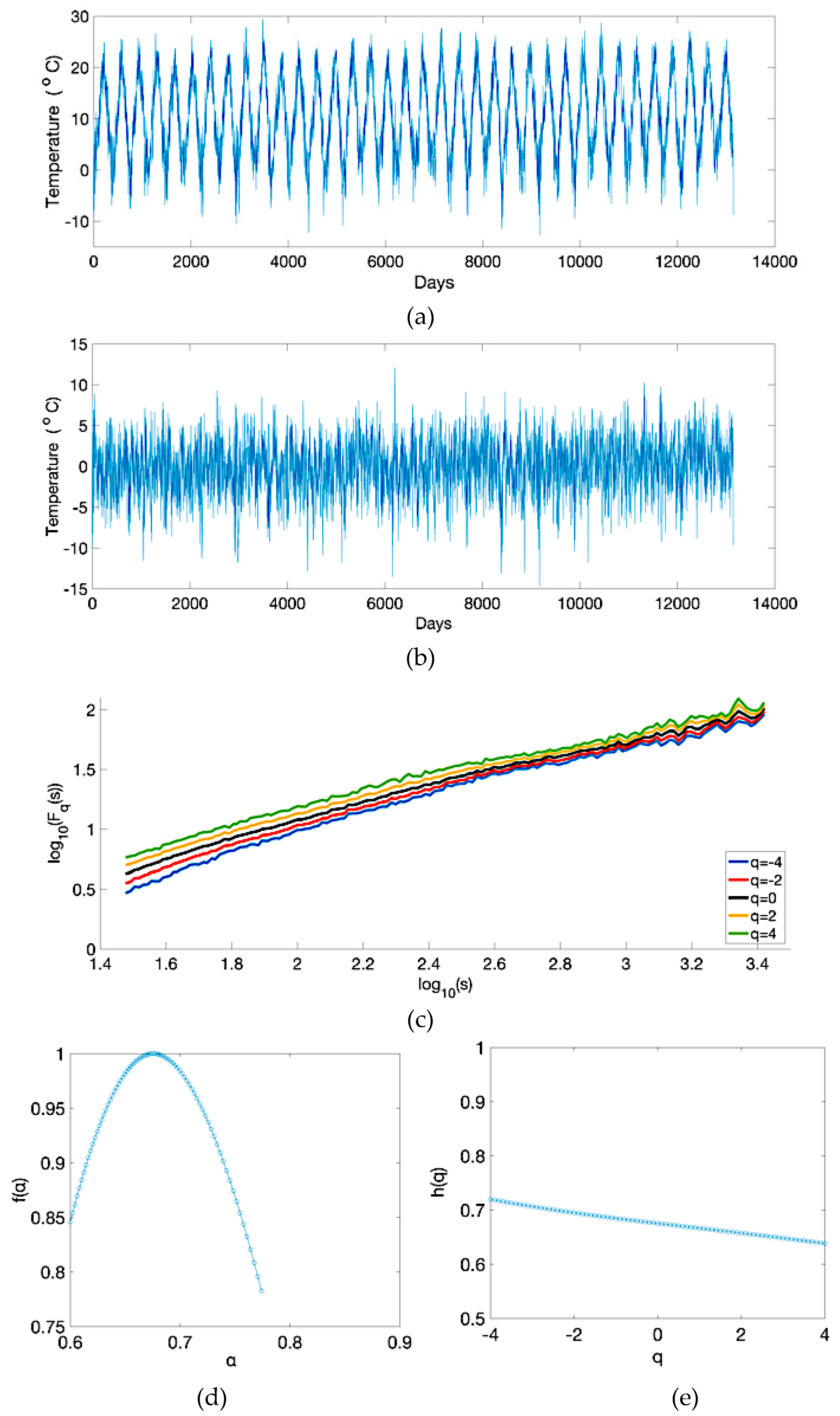
The application of the MF-DFA to the daily temperature for each grid point (154 time series), yields to the plots of the fluctuation factor Fq(s) versus times scale s, the generalized Hurst exponent h(q) versus q, and the multifractal spectrum f(α) versus α. In Figure 2 and Figure 3, these plots are presented along with the original and deseasonalized time series for the closest grid point to Athens (38.25° N, 24.00° E) and Kastoria (40.50° N, 21.00° E), respectively.
These grid points represent geographic areas with different climatic conditions. The grid point that is close to Athens is a coastal point, located in southeastern central Greece, and therefore it is influenced by the sea. On the other hand, the second grid point, which is located in mountainous northwestern Greece, is not influenced by the sea characterized by a colder climate. This is clearly reflected in Figure 2a and Figure 3a, where below-zero temperatures are often observed, especially during winter in northwestern Greece. The scaling behavior is determined by the fluctuation functions Fq(s) (Figure 2c and Figure 3c), which is similar in both grid points. The generalized Hurst exponent is greater than 0.5 in the two cases, revealing the fact that the temperature time series are long-range positively correlated. The most striking differences can be seen in the values of h(q), which are greater for the point located near to Athens (Figure 2e and Figure 3e). In addition to this, from Figure 2d and Figure 3d, it is observed that the value of α for which f(α) is maximum is greater for the point located near to Athens. This fact can be attributed to the influence of the sea, which leads to a more persistent behavior (that is, greater scaling exponents) as will be stated in the next paragraph. Moreover, the spectrum of the mountainous area (Figure 3d) is narrower than the spectrum of Figure 2d. This can be attributed to the complex topography of the mountainous areas, which is the cause of local weather conditions that, in turn, make temperature fluctuations to be noisier; a time series that has a structure similar to white noise has a narrow spectrum [56,57].
It should be noted that Fq(s) is plotted for s ranging from 101.5 to 103.5 in days. In all cases, the form of Fq(s) plots is almost linear, and, for different q values, their distance is decreased when s increases. This is attributed to the fact that, for small segments (small s values), local periods with small fluctuations (negative q) are easier to distinguish from periods with large fluctuations (positive q). On the contrary, large segments include periods of both small and large fluctuations and therefore the differences in magnitude are cancelled [56]. This results in the behavior of Fq(s) for large segments being similar to monofractal time series (i.e., the Fq(s) for monofractal time series is independent of q and in that case the Fq(s) lines coincide). The multifractal character of the temperature time series is exhibited from the fact that the Hurst exponent is dependent on q (Figure 2d) and from the upside-down parabola form of the multifractal spectrum (Figure 2e). In more detail, in all cases h(q) > 0.5, and consequently the temperature time series are long-range positively correlated and therefore it is highly likely that an increase/decrease in temperature values will be followed by another increase/decrease.
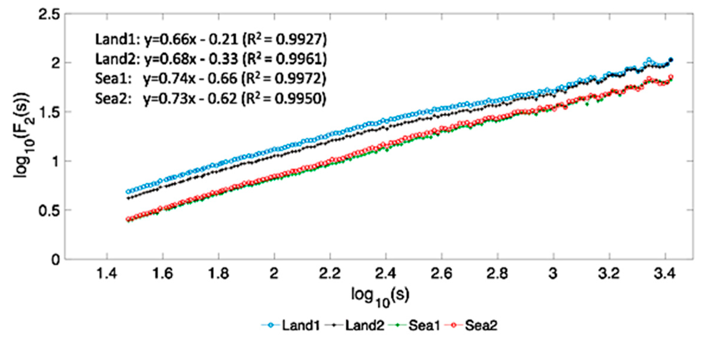
In Figure 4, the log-log plots of F2(s) versus s are illustrated for two representative grid points located over land (Land1: 39.75° N, 21.75° E, Land2: 37.50° N, 22.50° E) and for two points over sea (Sea1: 35.25° N, 27.75° E, Sea2: 36.75° N, 21.00° E). For each plot, a linear equation of the form y = ax + b is fitted, where a is the scaling exponent. It should be noted that, in all cases, high goodness-of-fit is achieved with coefficient of determination values greater than 99%. The estimated scaling exponents over sea are higher due to the influence of the higher seawater heat capacity, which leads to temperature time series with a higher degree of persistence. Furthermore, the lower F2(s) values over sea can be attributed to the smaller temperature fluctuations.
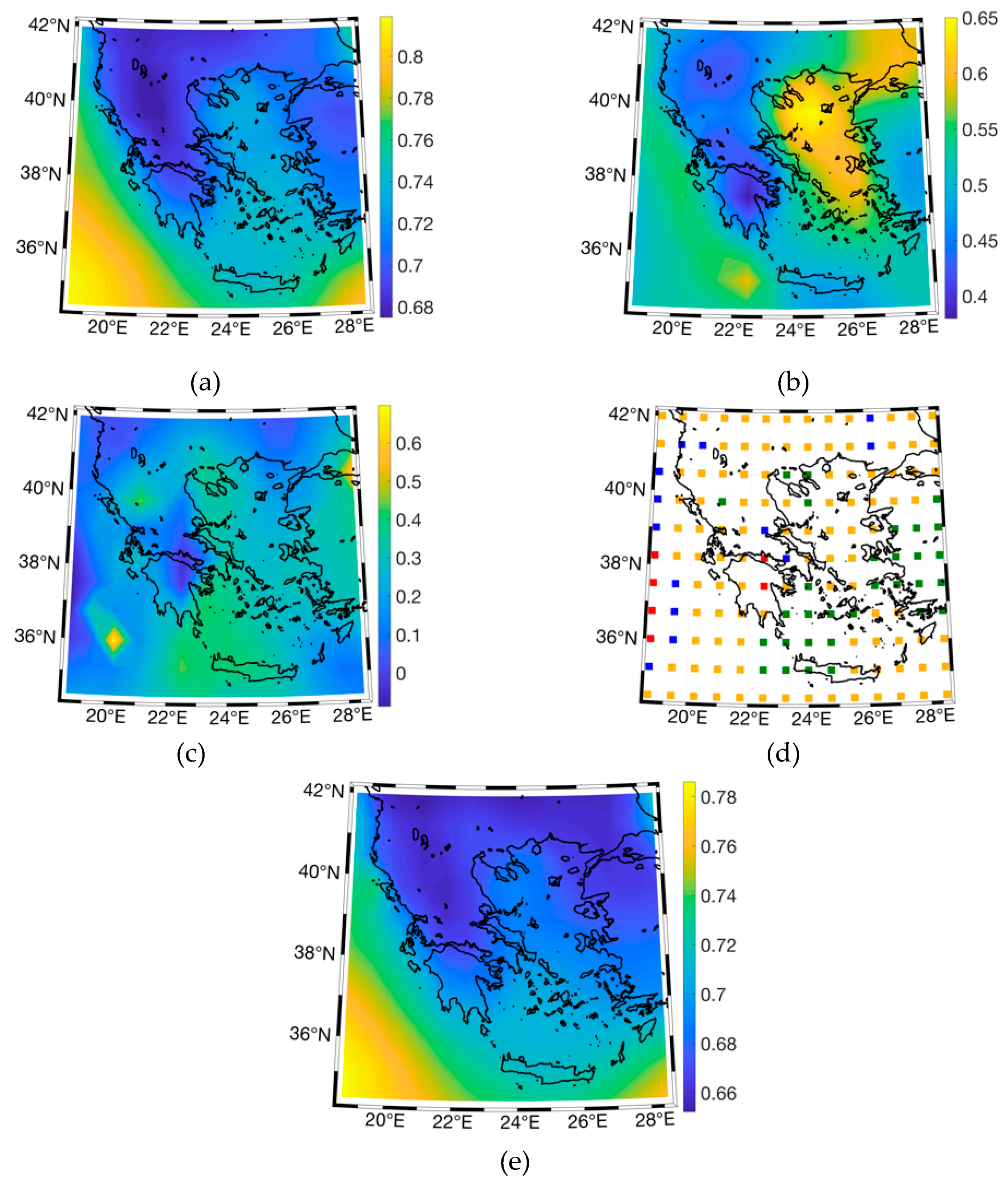
The multifractal characteristics, deducted from the multifractal spectrum (i.e., αmaxαmin width, α0, asymmetry parameter B, and truncation type), reveal important properties of the time series multifractality and their value distributions are illustrated in Figure 5. The α0 values range from 0.675 to 0.819 and, therefore, the dominant scaling exponent is greater than 0.5. In agreement with the h(q) findings, the dominant scaling behavior is persistent and positively correlated. The spectrum width values lie within the range of 0.380–0.650 and the asymmetry parameter values are in the range of −0.087–0.698. The B distribution demonstrates that the majority of the asymmetry values are positive and, therefore, in general, the spectra are right-skewed. As suggested by [57], a right-skewed spectrum shows relatively strongly weighted high fractal exponents (with a ‘fine structure’). Additionally, the examination of the truncation type of the spectra shows that the majority of the spectra are left-truncated, which is also indicative that, in general, there is a dominance of high fractal exponents.
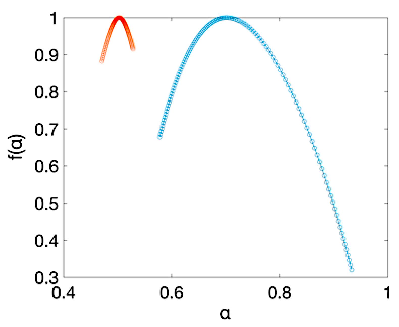
The type of multifractality of the temperature time series is examined by shuffling the time series and applying the MF-DFA to the shuffled time series. The results revealed that the shuffled time series exhibit a very weak multifractality and, therefore, the multifractality is caused mainly by different long-range correlations for small and large fluctuations. A representative case is depicted in Figure 6. In the multifractal spectrum of the shuffled time series, the value of α0 is very close to 0.5 and the spectrum width is clearly smaller than the corresponding width of the original time series.

4.2. Multifractal Characteristics Spatial Distribution

The spatial distributions of the multifractal characteristics are illustrated in Figure 7. Regarding the α0 spatial distribution (Figure 7a), the greater values are observed over marine areas, while lower values (darker color) dominate over land and, therefore, the time series exhibit a less persistent behavior over the continental areas of the domain. This finding could be attributed to the day-to-day variability of temperature, which is smaller over marine areas [59,60]. Over land, local weather conditions, such as katabatic winds, diabatic cooling or heating over ground, and the effect of elevation, lead to increased temperature variability. On the contrary, the greater heat capacity of seawater and the atmosphere–ocean interaction result in smaller changes in daily temperature. The same findings are also recognized in the spatial distribution of the Hurst exponent h(2) (Figure 7e). The spatial distribution of spectral width (Figure 7b) is very similar to that of α0. This can be attributed to the effect of complex terrain on local weather conditions, where temperature changes act as ‘noise’ to the smoother temperature changes caused by synoptic weather systems over land and to the effect of the sea over marine areas, where temperature changes exhibit a more persistent behavior.
The spatial distribution of the asymmetry parameter (Figure 7c) exhibits lower values over a part of continental Greece. This could be attributed to the fact that local weather parameters have a ‘noisy’ contribution to the multifractal spectrum, where the existence of low fractal exponents cancels out the right skewness caused by high fractal exponents. Additionally, the asymmetry parameter has, in general, higher values over the Aegean Sea than over other marine areas. This could be explained partially by the persistence of the Etesian winds [61] during summer, which affects accordingly the temperature field over the Aegean Sea. A similar situation is observed at the spatial distribution of truncation type (Figure 7d), where areas with lower values of asymmetry parameters appear to have a symmetrical or right-truncated spectrum.

5. Discussion

An additional scope of this study is to compare the scaling behavior of the reanalysis temperature time series with the corresponding findings from observational records from 22 land-based meteorological stations presented in [49]. The multifractal spectral parameters from the observational records and those from their nearest reanalysis data grid points are illustrated in Table 1. For the reader’s convenience, the station names and the corresponding nearest grid points are also given in Table 1. In all cases, the α0 differences are small (below 10%) and, therefore, the scaling behavior is virtually the same in both cases. Regarding the spectral width and the asymmetry parameters, greater differences between the two datasets are observed, which could be attributed mainly to the method used in deriving the temperature time series.
More specifically, α0 values for the observational data are of the order of 0.7, which verifies the long-range positively correlated behavior of the temperature time series. However, the dependence of α0 on land–sea distribution, which is evident in the reanalysis data results, is not clearly observed in the results from observational records. The most persistent behavior for the observational records is observed at southeastern Greece and parts of coastal western Greece; these two areas have more stable climatic conditions in Greece [50]. The range of spectrum width values is almost the same for the observational and reanalysis data, but likewise to α0, the role of land–sea distribution is not clearly detected. In addition, the behavior of the shuffled observational and reanalysis data is the same, which means that the multifractality is mainly due to different long-range correlations for different magnitudes of fluctuations.
Regarding the asymmetry parameter and truncation type spatial distributions, the reanalysis data findings are in accordance with the observational records results (positive values dominate in the experimental domain). The close relationship between the asymmetry parameter and truncation type, though it is not straightforward, is verified by Table 2. In general, left-truncated spectra are related to higher asymmetry parameter values than right-truncated spectra. In the latter case, the values of the asymmetry parameter are negative.
Another reason for the differences in multifractal spectrum characteristics between the observational and reanalysis time series is that the area of the study is evenly covered in the case of ERA-Interim reanalysis by a grid of 154 points, whereas only 22 weather stations have been used for the observational data analysis, which are more sparsely and unevenly distributed.

6. Conclusions

The MF-DFA analysis of the ERA-Interim reanalysis temperature data revealed that the time series are long-range positively correlated. In particular, the spatial distribution of the α0 parameter reveals a clear influence from the land/sea distribution. Lower α0 values are observed over land, whereas higher values prevail over marine areas, where temperature exhibits a more persistent behavior. This could be attributed to the higher seawater heat capacity. Regarding the spectral width, it is observed that higher values are found over marine areas, whereas lower values dominate over land and, thus, temperature time series at marine areas exhibit a higher degree of multifractality compared to continental areas. This finding could be attributed to the greater temperature variations over land. Such behavior is closer to that of white noise, which has a narrow spectrum [56]. On the other hand, the behavior is more persistent over sea and, therefore, temperature time series over marine areas appear to have a greater number of spectral components with higher Hölder exponent values. Moreover, it was deduced from the shuffled data spectra that the multifractal spectrum width is significantly smaller (of the order of 0.2) compared to that of the original data. This means that the multifractality is mainly due to different long-range correlations for different magnitudes of fluctuations. The values of the asymmetry parameter are positive in almost all areas (right-skewed spectra), which is indicative of the presence of strongly weighted high fractal exponents [57]. This is also confirmed from the dominance of left-truncated spectra. Future work will be focused on examining the multifractal characteristics of additional climatic parameters from experimental and reanalysis datasets for using the results in applied climatology.

Author Contributions

Conceptualization, K.P., N.K., C.G.T. and D.D.; Methodology, K.P., N.K., C.G.T. and D.D.; Software, K.P., N.K., C.G.T., D.D. and I.K.; Validation, K.P., N.K., C.G.T., D.D. and I.K.; Formal Analysis, K.P., N.K., C.G.T., D.D. and I.K.; Investigation, K.P., N.K., C.G.T. and D.D.; Data Curation, K.P., N.K., C.G.T., D.D. and I.K.; Writing—original draft preparation, K.P., N.K., C.G.T., D.D. and I.K.; Writing—review and editing,.; K.P., N.K., C.G.T., D.D. and I.K.; Visualization, K.P., N.K. and I.K.; Visualization, K.P., N.K. and I.K.; Supervision, K.P., C.G.T and D.D.

Funding

This research received no external funding.

Conflicts of Interest

The authors declare no conflicts of interest.

References

  1. Mandelbrot, B.B. Fractals: Form, Chance and Dimension; Freeman: San Francisco, CA, USA, 1977. [Google Scholar]
  2. Mandelbrot, B.B. The Fractal Geometry of Nature; Freeman: San Francisco, CA, USA, 1982. [Google Scholar]
  3. Feder, J. Fractals; Plenum: New York, NY, USA, 1988. [Google Scholar]
  4. Barnsley, M.F. Fractals Everywhere; Academic Press: San Diego, CA, USA, 1993. [Google Scholar]
  5. Mandelbrot, B.B. Multifractals and 1/f Noise: Wild Self-Affinity in Physics; Springer: Berlin, Germany, 1999. [Google Scholar]
  6. Kandelhardt, J.W. Fractal and Multifractal Time Series. In Mathematics of Complexity and Dynamical Systems; Meyers, R.A., Ed.; Springer: New York, NY, USA, 2011; pp. 463–487. [Google Scholar]
  7. Peng, C.K.; Buldyrev, S.V.; Havlin, S.; Simons, M.; Stanley, H.E.; Goldberger, A.L. Mosaic organization of DNA nucleotides. Phys. Rev. E 1994, 49, 1685–1689. [Google Scholar] [CrossRef] [Green Version]
  8. Kandelhardt, J.W.; Koscielny-Bunde, E.; Rego, H.A.H.; Havlin, S.; Bunde, A. Detecting long-range correlations with detrended fluctuation analysis. Physica A 2001, 295, 441–454. [Google Scholar] [CrossRef] [Green Version]
  9. Liu, Y.; Cizeau, P.; Meyer, M.; Peng, C.K.; Stanley, H.E. Correlations in economic time series. Physica A 1997, 245, 437–440. [Google Scholar] [CrossRef] [Green Version]
  10. Di Matteo, T.; Aste, T.; Dacorogna, M.M. Scaling behaviors in differently developed markets. Physica A 2003, 324, 183–188. [Google Scholar] [CrossRef]
  11. Barbi, M.; Chillemi, S.; Di Garbo, A.; Balocchi, R.; Carpeggiani, C.; Emdin, M.; Michelassi, C.; Santarcangelo, E. Predictability and nonlinearity of the heart rhythm. Chaos Soliton Fract. 1998, 9, 507–515. [Google Scholar] [CrossRef]
  12. Buldyrev, S.V.; Dokholyan, N.V.; Goldberger, A.L.; Havlin, S.; Peng, C.K.; Stanley, H.E.; Viswanathan, G.M. Analysis of DNA sequences using methods of statistical physics. Physica A 1998, 249, 430–438. [Google Scholar] [CrossRef]
  13. Gao, J.; Hu, J.; Mao, X.; Perc, M. Culturomics meets random fractal theory: Insights into long-range correlations of social and natural phenomena over the past two centuries. J. Royal Soc. Interface 2012, 9, 1956–1964. [Google Scholar] [CrossRef]
  14. Varotsos, C.A.; Melnikova, I.; Efstathiou, M.N.; Tzanis, C. 1/f noise in the UV solar spectral irradiance. Theor. Appl. Climatol. 2013, 111, 641–648. [Google Scholar] [CrossRef]
  15. Chattopadhyay, G.; Chattopadhyay, S. Study on statistical aspects of monthly sunspot number time series and its long-range correlation through detrended fluctuation analysis. Indian J. Phys. 2014, 88, 1135–1140. [Google Scholar] [CrossRef]
  16. Holton, J.R. An introduction to Dynamic Meteorology, 4th ed.; Elsevier Academic Press: Cambridge, MA, USA, 2004. [Google Scholar]
  17. Koscielny-Bunde, E.; Bunde, A.; Havlin, S.; Goldreich, Y. Analysis of daily temperature fluctuations. Physica A 1996, 231, 393–396. [Google Scholar] [CrossRef]
  18. Eichner, J.F.; Koscielny-Bunde, E.; Bunde, A.; Havlin, S.; Schellnhuber, H.J. Power-law persistence and trends in the atmosphere: A detailed study of long temperature records. Phys. Rev. E 2003, 68, 046133. [Google Scholar] [CrossRef] [PubMed] [Green Version]
  19. Bartos, I.; Janosi, I.M. Nonlinear correlations of daily temperature records over land. Nonlinear Proc. Geophys. 2006, 13, 571–576. [Google Scholar] [CrossRef] [Green Version]
  20. Orun, M.; Koçak, K. Application of detrended fluctuation analysis to temperature data from Turkey. Int. J. Climatol. 2009, 29, 2130–2136. [Google Scholar] [CrossRef]
  21. Yuan, N.; Fu, Z.; Mao, J. Different scaling behaviors in daily temperature records over China. Physica A 2010, 389, 4087–4095. [Google Scholar] [CrossRef]
  22. Kalamaras, N.; Philipppopoulos, K.; Deligiorgi, D. Scaling Properties of Meteorological Time Series Using Detrended Fluctuation Analysis. In Perspectives on Atmospheric sciences, Proceedings of the 13th International Conference of Meteorology, Climatology and Atmospheric Physics, Thessaloniki, Greece, 19–21 September 2016; Karacostas, T.S., Bais, A.F., Nastos, P.T., Eds.; Springer Atmospheric Physics; Springer International Publishing: Cham, Switzerland, 2016; pp. 545–550. [Google Scholar]
  23. Podobnik, B.; Ivanov, P.C.; Jazbinsek, V.; Trontelj, Z.; Stanley, H.E.; Grosse, I. Power-law correlated processes with asymmetric distributions. Phys. Rev. E 2005, 71, 025104. [Google Scholar] [CrossRef] [PubMed]
  24. Lin, G.; Chen, X.; Fu, Z. Temporal–spatial diversities of long-range correlation for relative humidity over China. Physica A 2007, 383, 585–594. [Google Scholar] [CrossRef]
  25. Jiang, L.; Zhao, L.; Zhao, Z. On the Difference of Scaling Properties for Temperature and Precipitation over China. Adv. Meteorol. Hindawi 2017, 2017. [Google Scholar] [CrossRef]
  26. He, W.; Zhao, S.; Liu, Q.; Jiang, Y.; Deng, B. Long-range correlation in the drought and flood index from 1470 to 2000 in eastern China. Int. J. Climatol. 2016, 36, 1676–1685. [Google Scholar] [CrossRef]
  27. Varotsos, C.A.; Tzanis, C. A new tool for the study of the ozone hole dynamics over Antarctica. Atmos. Environ. 2012, 47, 428–434. [Google Scholar] [CrossRef]
  28. Varotsos, C.A.; Milinevsky, G.; Grytsai, A.; Efstathiou, M.; Tzanis, C. Scaling effect in planetary waves over Antarctica. Int. J. Remote Sens. 2008, 29, 2697–2704. [Google Scholar] [CrossRef]
  29. Varotsos, C.; Efstathiou, M.; Tzanis, C.; Deligiorgi, D. On the limits of the air pollution predictability: the case of the surface ozone at Athens, Greece. Environ. Sci. Pollut. Res. 2012, 19, 295–300. [Google Scholar] [CrossRef] [PubMed]
  30. Varotsos, C.; Tzanis, C.; Efstathiou, M.; Deligiorgi, D. Tempting long-memory in the historic surface ozone concentrations at Athens, Greece. Atmos. Pollut. Res. 2015, 6, 1055–1057. [Google Scholar] [CrossRef]
  31. Varotsos, C.A.; Lovejoy, S.; Sarlis, N.V.; Tzanis, C.G.; Efstathiou, M.N. On the scaling of the solar incident flux. Atmos. Chem. Phys. 2015, 15, 7301–7306. [Google Scholar] [CrossRef] [Green Version]
  32. Lovejoy, S. A voyage through scales, a missing quadrillion and why the climate is not what you expect. Clim. Dyn. 2015, 44, 3187–3210. [Google Scholar] [CrossRef]
  33. Caldeira, R.; Fernandez, I.; Pacheco, J.M. On NAO’s predictability through the DFA method. Meteorol. Atmos. Phys. 2007, 96, 221–227. [Google Scholar] [CrossRef]
  34. Kandelhardt, J.W.; Zschiegner, S.A.; Koscielny-Bunde, E.; Havlin, S.; Bunde, A.; Stanley, H.E. Multifractal detrended fluctuation analysis of nonstationary time series. Physica A 2002, 316, 87–114. [Google Scholar] [CrossRef] [Green Version]
  35. Lovejoy, S.; Schertzer, D. The Weather and Climate Emergent Laws and Multifractal Cascades; Cambridge University Press: New York, NY, USA, 2013. [Google Scholar]
  36. Kalamaras, N.; Philippopoulos, K.; Deligiorgi, D.; Tzanis, C.G.; Karvounis, G. Multifractal scaling properties of daily air temperature time series. Chaos Solitons Fractals. 2017, 98, 38–43. [Google Scholar] [CrossRef]
  37. Svensson, C.; Olsson, J.; Berndtsson, R. Multifractal properties of daily rainfall in two different climates. Water Resour. Res. 1996, 332, 2463–2472. [Google Scholar] [CrossRef]
  38. Du, H.; Wu, Z.; Zong, S.; Meng, X.; Wang, L. Assessing the characteristics of extreme precipitation over northeast China using the multifractal detrended fluctuation analysis. J. Geophys. Res. Atmos 2013, 118, 6165–6174. [Google Scholar] [CrossRef]
  39. Shao, Z.-G.; Ditlevsen, P. Contrasting scaling properties of interglacial and glacial climates. Nat. Commun. 2016, 7, 10951. [Google Scholar] [CrossRef] [Green Version]
  40. Zhang, X.; Zhang, G.; Qiu, L.; Zhang, B.; Sun, Y.; Gui, Z.; Zhang, Q. A Modified Multifractal Detrended Fluctuation Analysis (MFDFA) Approach for Multifractal Analysis of Precipitation in Dongting Lake Basin, China. Water 2019, 11, 891. [Google Scholar] [CrossRef]
  41. Kavasseri, R.G.; Nagarajan, R. A multifractal description of wind speed records. Chaos Soliton Fract. 2005, 24, 165–173. [Google Scholar] [CrossRef]
  42. Feng, T.; Fu, Z.; Deng, X.; Mao, J. A brief description to different multi-fractal behaviors of daily wind speed records over China. Phys. Lett. A 2009, 373, 4134–4141. [Google Scholar] [CrossRef]
  43. Laib, M.; Telesca, L.; Kanevski, M. Long-range fluctuations and multifractality in connectivity density time series of a wind speed monitoring network. Chaos 2018, 28, 033108. [Google Scholar] [CrossRef] [PubMed] [Green Version]
  44. Pedron, I.T. Correlation and multifractality in climatological time series. J. Phys. Conf. Ser. 2010, 246, 012034. [Google Scholar] [CrossRef]
  45. Baranowski, P.; Krzyszczak, J.; Slawinski, C.; Hoffmann, H.; Kozyra, J.; Nieróbca, A.; Siwek, K.; Gluza, A. Multifractal analysis of meteorological time series to assess climate impacts. Clim. Res. 2015, 65, 39–52. [Google Scholar] [CrossRef]
  46. Hoffmann, H.; Baranowski, P.; Krzyszczak, J.; Zubik, M.; Sławiński, C.; Gaiser, T.; Ewert, F. Temporal properties of spatially aggregated meteorological time series. Agric. Forest Meteorol. 2017, 234–235, 247–257. [Google Scholar]
  47. Krzyszczak, J.; Baranowski, P.; Zubik, M.; Hoffmann, H. Temporal scale influence on multifractal properties of agro-meteorological time series. Agric. Forest Meteorol. 2017, 239, 223–235. [Google Scholar] [CrossRef]
  48. Xue, Y.; Pan, W.; Lu, W.; He, H. Multifractal nature of particulate matters (PMs) in Hong Kong urban air. Sci. Total Environ. 2015, 532, 744–751. [Google Scholar] [CrossRef]
  49. Kalamaras, N.; Tzanis, C.G.; Deligiorgi, D.; Philippopoulos, K.; Koutsogiannis, I. Distribution of air temperature multifractal characteristics over Greece. Atmosphere 2019, 10, 45. [Google Scholar] [CrossRef]
  50. Mariolopoulos, E.G. The Climate of Greece; A.A. Papaspyrou Press: Athens, Greece, 1938. (In Greek) [Google Scholar]
  51. Karras, G. Climatic Classification of Greece According to Thornthwaite. Ph.D. Thesis, National and Kapodistrian University of Athens, Athens, Greece, 1973. (In Greek). [Google Scholar]
  52. Feidas, H.; Makrogiannis, T.; Bora-Senta, E. Trend analysis of air temperature time series in Greece and their relationship with circulation using surface and satellite data: 1955–2001. Theor. Appl. Climatol. 2004, 79, 185–208. [Google Scholar] [CrossRef]
  53. Dee, D.P.; Uppala, S.M.; Simmons, A.J.; Berrisford, P.; Poli, P.; Kobayashi, S.; Andrae, U.; Balmaseda, M.A.; Balsamo, G.; Bauer, P.; et al. The ERA-Interim reanalysis: Configuration and performance of the data assimilation system. Q. J. Royal Meteorol. Soc. 2011, 137, 553–597. [Google Scholar] [CrossRef]
  54. Berrisford, P.; Dee, D.; Poli, P.; Brugge, R.; Fielding, K.; Fuentes, M.; Kallberg, P.; Kobayashi, S.; Uppala, S.; Simmons, A. The ERA-Interim Archive, version 2.0; ERA Report Series; ECMWF Publications: Reading, UK, 2011. [Google Scholar]
  55. Bishop, S.M.; Yarham, S.I.; Navapurkar, V.U.; Menon, D.K.; Ercole, A. Multifractal analysis of hemodynamic behavior: Intraoperative instability and its pharmacological manipulation. Anesthesilogy 2012, 117, 810–821. [Google Scholar] [CrossRef] [PubMed]
  56. Ihlen, E.A.F. Introduction to multifractal detrended fluctuation analysis in Matlab. Front. Physiol. 2012, 3, 141. [Google Scholar] [CrossRef] [PubMed]
  57. Shimizu, Y.; Thurner, K.; Ehrenberger, K. Multifractal spectra as a measure of complexity in human posture. Fractals 2002, 10, 103–116. [Google Scholar] [CrossRef]
  58. Burgueno, A.; Lana, X.; Serra, C.; Martinez, M.D. Daily extreme temperature multifractals in Catalonia (NE Spain). Phys. Lett. A 2014, 378, 874–885. [Google Scholar] [CrossRef]
  59. Bountas, N.; Boboti, N.; Feloni, E.; Zeikos, L.; Markonis, Y.; Tegos, A.; Mamassis, N.; Koutsoyiannis, D. Temperature variability over Greece: Links between space and time. In Proceedings of the 5th EGU Leonardo Conference, Kos Island, Greece, 17–19 October 2013. [Google Scholar]
  60. Stathopoulos, V.; Fotiadi, A.; Houssos, E.E.; Hatzianastassiou, N.; Vardavas, I. Day to Day Variability of Air Temperature over Greece for the Period 1957–2002. In Advances in Meteorology, Climatology and Atmospheric Physics; Springer Atmospheric Sciences; Springer: erlin/Heidelberg, Germany, 2012; pp. 737–742. [Google Scholar]
  61. Metaxas, D.A. The interannual variability of the Etesian frequency as a response of atmospheric circulation anomalies. Bull Hell Meteorol. Soc. 1977, 2, 30–40. [Google Scholar]
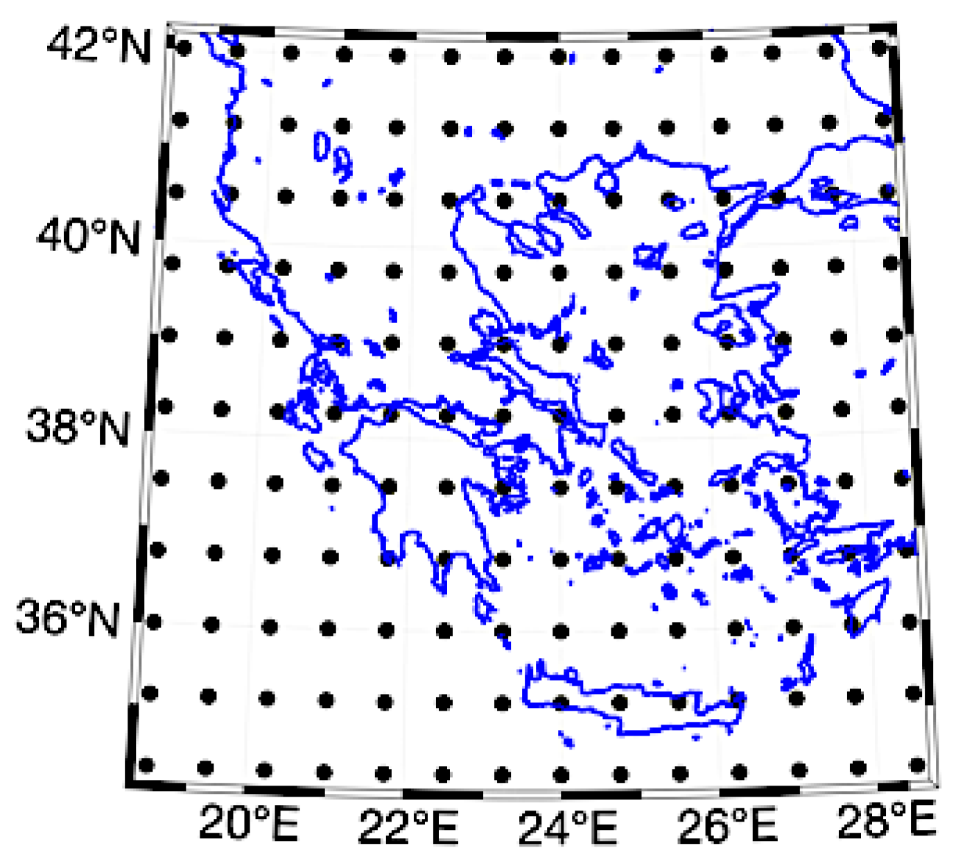
Figure 1. The area of study and the ERA-Interim reanalysis grid points.
Atmosphere 10 00336 g001
Figure 2. Original time series (a), deseasonalized time series (b), log-log plot of Fq(s) versus s (c), multifractal spectrum f(α) versus α for the nearest grid point to Athens (38.25° N, 24.00° E) (d) and generalized Hurst exponent h(q) versus q plot (e)
Atmosphere 10 00336 g002
Figure 3. Original time series (a), deseasonalized time series (b), log-log plot of Fq(s) versus s (c), multifractal spectrum f(α) versus α for the nearest grid point to Kastoria (40.50° N, 21.00° E) (d) and generalized Hurst exponent h(q) versus q plot (e).
Atmosphere 10 00336 g003
Figure 4. Log-log plots of F2(s) for two grid points located over land (Land1: 39.75° N, 21.75° E, Land2: 37.50° N, 22.50°E) and for two points located over sea (Sea1: 35.25° N, 27.75° E, Sea2: 36.75° N, 21.00° E) along with the linear fit equations and the corresponding coefficient of determination R2 values.
Atmosphere 10 00336 g004
Figure 5. Multifractal spectral parameters distributions for a0 (a), spectral width (b), asymmetry parameter (c), and truncation type (d).
Atmosphere 10 00336 g005
Figure 6. Multifractal spectra for the original (right) and for the shuffled (left) time series. The plots are for the closest to Thessaloniki grid point (40.50° N, 23.25° E).
Atmosphere 10 00336 g006
Figure 7. Spatial distribution of a0 (a), spectral width (b), asymmetry parameter (c), truncation type (d) where (LL: green squares, L: orange squares, S: blue squares, and R: red squares), and h(2) (e).
Atmosphere 10 00336 g007
Table 1. Spectral parameters’ values of observational (Obs) and ERA-Interim (ERA) time series for the closest to the station grid points.
StationNearest Pointα0Spectral WidthAsymmetry Parameter
ObsERAObsERAObsERA
Alexandroupoli40.50° N, 26.25° E0.6850.7140.5450.6000.1800.177
Andravida38.25° N, 21.00° E0.7200.7190.6640.5020.4960.291
Elefsina38.25° N, 23.25° E0.7080.7050.6290.4410.4160.086
Hellinikon38.25° N, 24.00° E0.7190.7250.6590.5320.3990.344
Herakleio35.25° N, 25.50° E0.7120.7440.4580.4840.3750.362
Kastoria40.50° N, 21.00° E0.7130.6750.4790.4210.0380.252
Kerkira39.75° N, 20.25° E0.7120.6900.4470.4420.2240.272
Kithira36.00° N, 23.25° E0.6880.7410.3880.4980.4970.384
Kos36.75° N, 27.00° E0.7470.7370.5110.5490.0370.270
Lamia39.00° N, 22.50° E0.7180.6890.5000.4460.4780.066
Larisa39.75° N, 22.50° E0.6840.6930.6590.4660.6850.105
Limnos39.75° N, 25.50° E0.7250.7240.5660.6200.2550.218
Methoni36.75° N, 21.75° E0.7340.7370.5480.4970.3960.283
Milos36.75° N, 24.75° E0.6960.7440.4700.5360.2140.340
Mitilini39.00° N, 26.25° E0.7150.7170.5320.5800.2690.259
Naxos36.75° N, 25.50° E0.7750.7440.6770.5530.3050.297
Preveza39.00° N, 21.00° E0.7200.6950.7270.4260.5770.087
Rodos36.00° N, 27.75° E0.7300.7560.4370.5230.0970.161
Skiros39.00° N, 24.75° E0.7030.7310.5440.6150.4090.271
Souda35.25° N, 24.00° E0.6910.7450.6880.4900.2870.399
Thessaloniki40.50° N, 23.25° E0.7170.7020.4630.5210.2990.377
Tripoli37.50° N, 22.50° E0.7340.7010.3800.3800.317−0.029
Table 2. Range of asymmetry parameter values for each truncation type.
Truncation TypeAsymmetry Parameter
LL0.288–0.450
L0.033–0.698
S0.029–0.341
R−0.087–0.016