A New Approach for Generating Human Biometeorological Information Based on Gridded High-Resolution Data (Basic Data of Test-Reference-Years)

Abstract

The assessment of human-biometeorological information requires appropriate preparation of data and suitable visualisation of results. Human-biometeorological information can be valuable for tourists and visitors, but also for citizens looking for information about their neighbourhood or a new residence. Cities or health resorts can also promote their climate conditions for health rehabilitation. To derive this human-biometeorological information in a unified, comprehensive, and comprehensible form, a tool was developed. The input information contains the coordinates of a place and/or area of interest, and the time period of data chosen by the user. For meteorological data, the basic dataset of Test-Reference-Years from the German Meteorological Service is used, containing hourly meteorological data for the time period from 1995 to 2012, covering Germany with a spatial resolution of 1 km². Based on the Perceived Temperature as a thermal index, days with heat stress and cold stimulus are identified. In this process, the effects of short-term human acclimatisation on the thermal environment are considered by using a variable threshold value based on the thermal conditions of the last 30 days. The results of the tool’s application consist of several frequency diagrams, the Climate-Tourism/Transfer-Information-Scheme, a diagram of heat waves, and maps of the area of interest, displaying the spatial distribution of heat stress and cold stimulus. As an example, the (bio-)meteorological conditions of the region of southern Baden around Freiburg and the Black Forest, including the health resort, Hinterzarten, are analysed.

1. Introduction

The thermal complex plays a central role in human biometeorology, as the human body is permanently confronted with a thermal environment and challenged to keep a balanced heat exchange. Extreme heat and cold are stress factors that can have adverse consequences to health, e.g., heat strokes (e.g., [1,2,3]). However, slightly cold conditions can be used as a positive stimulation effect for climatotherapy [1]. Several approaches exist to capture the complexity of the human body´s heat exchange with the environment, generating an assessment index of thermal perception [4]. Examples of such thermal indices are the Perceived Temperature (PT) from the German Meteorological Service (Deutscher Wetterdienst, DWD) [5,6,7], the Physiologically Equivalent Temperature (PET) [8,9,10,11], and the Universal Thermal Climate Index (UTCI) [12].

The thermal perception of humans is influenced mainly by a combination of the meteorological variables of air temperature, humidity, wind speed, and radiation fluxes. The physiological factors influencing thermal perception are the metabolic rate, mechanical power, and the insulating effect of clothing. The human body´s thermoregulation system controls heat production and heat dissipation. The purpose of this control is to minimize the deviation of the core temperature from its standard value (37 °C) due to variant thermal conditions of the environment [13]. Thermal perception is comfortable if the activity of the thermoregulation is minimal, i.e., if the thermal conditions of the environment are within the thermal comfort zone. If the body is exposed to thermal conditions beyond this zone, the thermoregulation tries to balance out the additional heat gain or heat loss [14]. Extreme thermal conditions can lead to a dysfunctional thermoregulation system, with changes to the body’s core temperature. If the body´s core temperature falls below 28 °C (hypothermia), severe cardiac arrhythmias are possible, which can result in death. If the body core temperature rises above 41 °C (hyperthermia), important proteins and the brain can be damaged, and vasoconstriction and sweat production will be reduced. Damage from heat stroke is mostly irreversible and can lead to death. Even moderate heat or cold stress can have consequences on our health, especially if it continues over several days [14,15].

Understanding the physiological reaction to heat is essential to prevent heat related mortality, which is one of the main causes of weather related mortality [14]. The awareness of the danger of heat waves has risen in the last decades; extreme events like the European heat wave of 2003 led to the installation of Heat Health Warning Systems in many countries [16]. One of the factors determining heat tolerance beyond pre-existing illness is acclimatisation (ACC). The body can adapt to heat and cold when exposed to them for a few subsequent days. This includes both physiological and behavioural changes. If the adaption processes fail, the heat tolerance stays on a low level [14,17]. Therefore, the effect of acclimatisation is important to detect heat related mortality and should be considered in the assessment of thermal perception [14].

Further application areas of human biometeorology, besides the health sector including warnings of extreme events and the detection of positive effects for climatotherapy, are urban and regional planning and the tourism industry [18]. A lot of indices exist to assess weather conditions, especially in tourism. Tourism climate indices aim to give information about the best time and region with suitable weather conditions for tourism activity by combining several different meteorological, geographical, and seasonal factors [18,19]. The public and media are very interested in information about human biometeorology. Due to the research of the last decades, it is now possible to offer warnings, general information, and forecasts with high temporal and spatial resolution, accessible on websites, weather applications for smartphones, and newspapers [20]. Beyond access to the data, presenting these data in a relevant and understandable way is an important task. Besides the indices, there are other forms to visualize climatic information for the public. Maps can display the spatial distribution of a specific factor or condition, and diagrams with frequency distribution represent the climatic conditions of a specific place or region.

The choice of representing data is dependent on the availability and resolution of data. If the temporal resolution is high, yearly frequency distributions with a ten day period are possible (decades instead of monthly periods) [21,22]. For a climatic map of a city and its surroundings, the spatial resolution should be at least on a meso scale, which means a grid cell size of 1 km² [5]. For local maps on a micro scale, a higher spatial resolution is required [20].

The frequency and intensity of extreme weather events will increase in the future due to climate change [23,24]. Especially for temperature extremes on a global-scale, confidence in the expected long-term change is high [24]. Temperature extremes have a relatively high occurrence compared to other extreme events like droughts. Therefore, confidence in the observed changes allows this forecast. It is very likely that the overall number of cold days has decreased and the overall number of warm days and warm nights has increased [24]. To identify such trends, the current and past climate conditions have to be analysed. For this, reliable data for a preferably long time period (a standard of 30 years) are absolutely necessary. Meteorological data with high temporal and spatial resolution for a specific region like Germany make it possible to analyse the current situation of climate conditions and the occurrence of extreme events like heat waves.

This study focuses on the thermal complex of human biometeorology, analysing the frequency and spatial distribution of thermal perception classes like heat stress and cold stimulus, and representing the results with different diagrams and maps. The analyses are computed within a tool developed for this purpose, with an open and high-resolution dataset of the DWD. The tool is designed to generate and communicate nationwide bioclimatic information, providing a selection of different settings for choosing a favourite Point of Interest (POI) or Area of Interest (AOI) in Germany and the time period.

2. Data and Method

2.1. Data

The data used for the analyses is the so-called “basis dataset of the Test-Reference-Years” (TRY) from the German Meteorological Service [25]. This is a gridded dataset covering the German land surface and comprises the following 12 meteorological variables: air temperature (T_a), air pressure (P), dew point temperature (T_d), cloud cover (CC), relative humidity (RH), water vapour content (X), wind speed (v) and wind direction (WD), global (G) and direct radiation (SIS), and both surface down-welling (SDL) and up-welling longwave radiation (SOL). The dataset covers the years from 1995 to 2012 with a spatial resolution of 1 km² and a temporal resolution of one hour [25]. Different data sources were used to construct the gridded data. The main source was data from synoptic stations. Measurements from satellites provide data for the radiation components and cloud cover used to eliminate the influence of topographic barriers like mountain ranges and strong winds on cloud patterns. To support the gridding of the wind and longwave radiation components, downscaled reanalysis data from a regional climate model (RCM) [26] was used (

Table 1. Meteorological variables and data sources used for the gridding procedure of basis dataset of TRY [25]. RCM, Regional Climate Model.

Climate Variable	Unit	Station Data	Satellite Data	RCM Data
Air temperature	°C	X
Air pressure	hPa	x
Dew point temperature	°C	X
Relative humidity	%	X
Water vapour content	g/Kg	X
Cloud cover	1/8	X	X
Global radiation	W/m2	X	X
Direct radiation	W/m2	X	X
Down-welling longwave radiation	W/m2		X	X
Up-welling longwave radiation	W/m2		X	X
Wind speed	m/s	X		X
Wind direction	°	X		X

).

The gridding procedure was used with different methods of interpolation, depending on the data source, data density, and the climate variable. For more details about the data gridding process and interpolation see [25].

As a consequence of the high spatial and temporal resolution, the effect of the Urban Heat Island (UHI) has to be considered [25]. The UHI effect is reflected in the positive difference of air temperature between urban and rural areas. This difference is the mutual response of urban factors, such as anthropogenic heat storage building material and its specific albedo [27,28]. Therefore, the UHI effect is integrated into the gridding process of air temperature fields.

Another effect of urban climate is the difference of humidity between urban and rural areas. In general, relative humidity is reduced in urban areas, with a maximum of more than 15% during the night [29,30,31]. Reasons for this effect are the reduced latent heat flux and the higher T_a in urban areas compared to rural ones. Since RH is dependent on T_a, water vapour pressure (VP) should be examined, too. In calm and cloudless summer nights, VP can be increased in cities despite a lower relative humidity [30,31]. Both effects were only considered by the interpolation of dew point and air temperature [25].

The statistical evaluation of the data grids (with a leave-one-out cross-validation, as per [25]) reveals a high root mean square error (averaged RMSE over data time period 1995–2012) for wind speed, direct, and global radiation. The satellite-derived radiation parameters are underestimated due to snow cover, which can be misinterpreted as clouds. The same misinterpretation leads to an overestimation of cloud cover between 0.5 to 1.2 eights, especially in winter. Wind speed is spatially highly heterogeneous, and particularly low wind speed is difficult to measure with wind sensors. Thus, the predicted data delineate an overestimation of low wind speed (about 1 m/s) compared to the observed data. The hourly air temperature prediction depicts an error of about 1 °C, with higher errors in regions with complex terrain. Comparing the distribution of the cross-validated predicted data with the observed data, the air temperature grids match over the entire value range and all regions in Germany. Further, the long-term averages of hourly radiation also match. Relative humidity shows an overestimation in the lower section of predicted distribution of nearly 5% [25].

The presented dataset was initially generated to update the Test-Reference-Years of Germany, an artificial dataset for technical climatology with hourly data for the length of one year (365 days), first developed in 1986 (and updated several times). This dataset consists of observational data of several meteorological parameters and describes the annual cycle, but also shorter sections from one day up to a length of one month. The main applications of the TRY data are in technical air conditioning systems and as input for thermal building simulations to estimate energy consumption. Because of the size and different climate regions of Germany, the TRY data were divided into 15 climate regions, with one meteorological station representing each region. Thus, the TRY data did not have the same representative status in the German regions. With the new dataset for every square kilometre, various applications emerged. The 1 km² hourly gridded dataset is now the basis of the new TRY and publicly available from the DWD Climate Data Center CDC [32].

2.2. Method

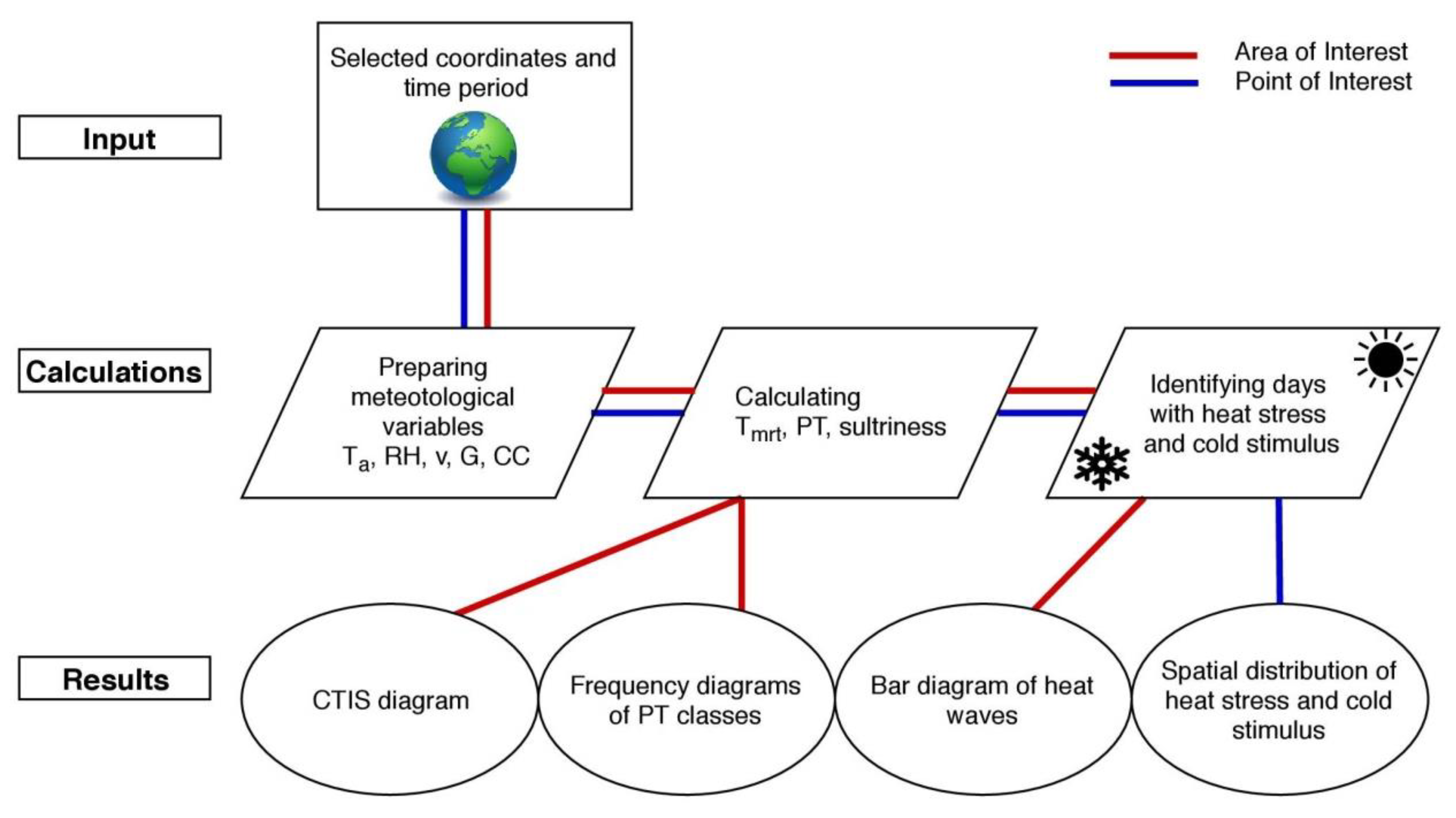
2.2.1. Calculation Procedure

The calculation procedure of the developed tool consists of eight calculation and analysis steps implemented in R scripts (Figure 1). The coordinates of the selected Point or Area of Interest (POI or AOI), and the chosen time periods are the input information with which the required meteorological data will be selected from the TRY basis dataset. The next steps are the calculation of wind speed at a 1.1 m height (v_1.1), VP, the calculation of mean radiant temperature (T_mrt), PT, and sultriness. In the following analysis, the days with heat stress and cold stimulus are identified. The results are presented with graphics depending on the requested data (POI or AOI). If information for a POI is requested, a Climate-Tourism/Transfer-Information-Scheme [33,34], frequency diagrams of PT classes, and a bar diagram that displays occurring heat waves are returned as output. If an AOI was selected, the output contains maps of the requested regions with the number of days with heat stress and cold stimulus for each 1 km² cell. All calculation steps, the generating, naming, and saving of results proceed by default.

After the input is completed, meteorological data of the requested time period and area can be extracted. In order to calculate PT, at least four meteorological variables are needed: T_a, RH, v, CC, and/or G. Both CC and G can be used to calculate T_mrt individually [9,35,36]. If both of them are available, they can supplement the calculation.

The wind speed data provided represents the standard measurement height of 10 ± 4 m. However, for the calculation of T_mrt and PT, wind speed at the height of the average human gravity centre of 1.1 m is relevant. To convert the wind speed, the wind profile of [37] and [38] is used.

For the calculation of T_mrt, the approach according to [36], taken from the RayMan model, is implemented. The following adjustments due to the data structure and availability (interpolated data of 1 km²) are necessary: the default value for human albedo = 0.3 after [39,40], the albedo of the surroundings α = 0.2, the Bowen ratio = 1, the emissivity of the surroundings and the sky view factor svf = 1. The Bowen ratio describes the ratio between latent and sensible heat transfer. To estimate the turbidity of atmosphere, the Linke turbidity is considered [36].

Input parameters for computing T_mrt in the tool are T_a, VP, G, and CC, v_1.1, the geographical coordinates and elevation, and the date and time. The calculation of Perceived Temperature is implemented as FORTRAN code that is executed from the R script. Input parameters are T_a, VP, v_1.1, and T_mrt. Outputs are the Perceived Temperature and an index (d_std) for sultriness in hourly resolution. This index for sultriness is defined according to [41]. With this, the index depicts the occurrence of sultriness affecting the PT in addition to the other parameters [42].

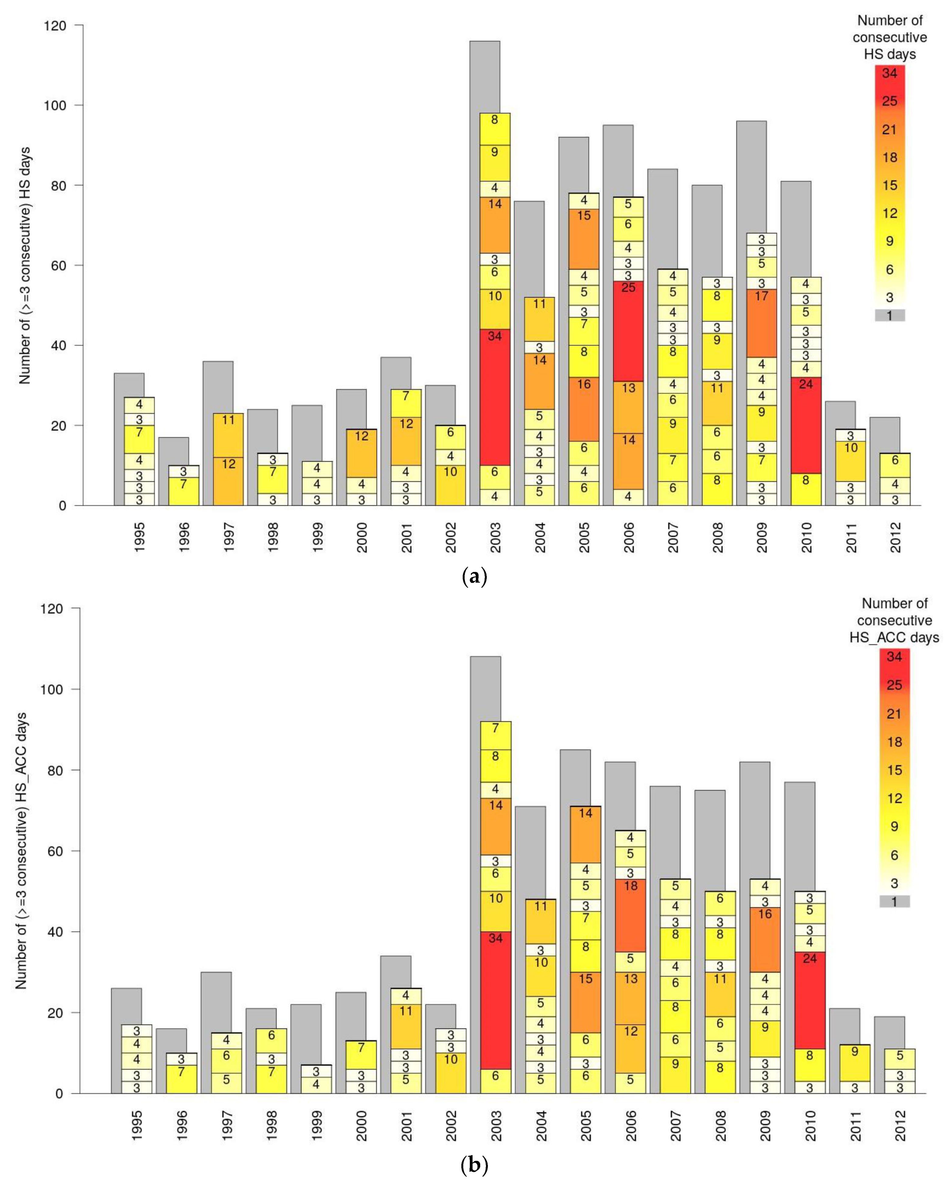
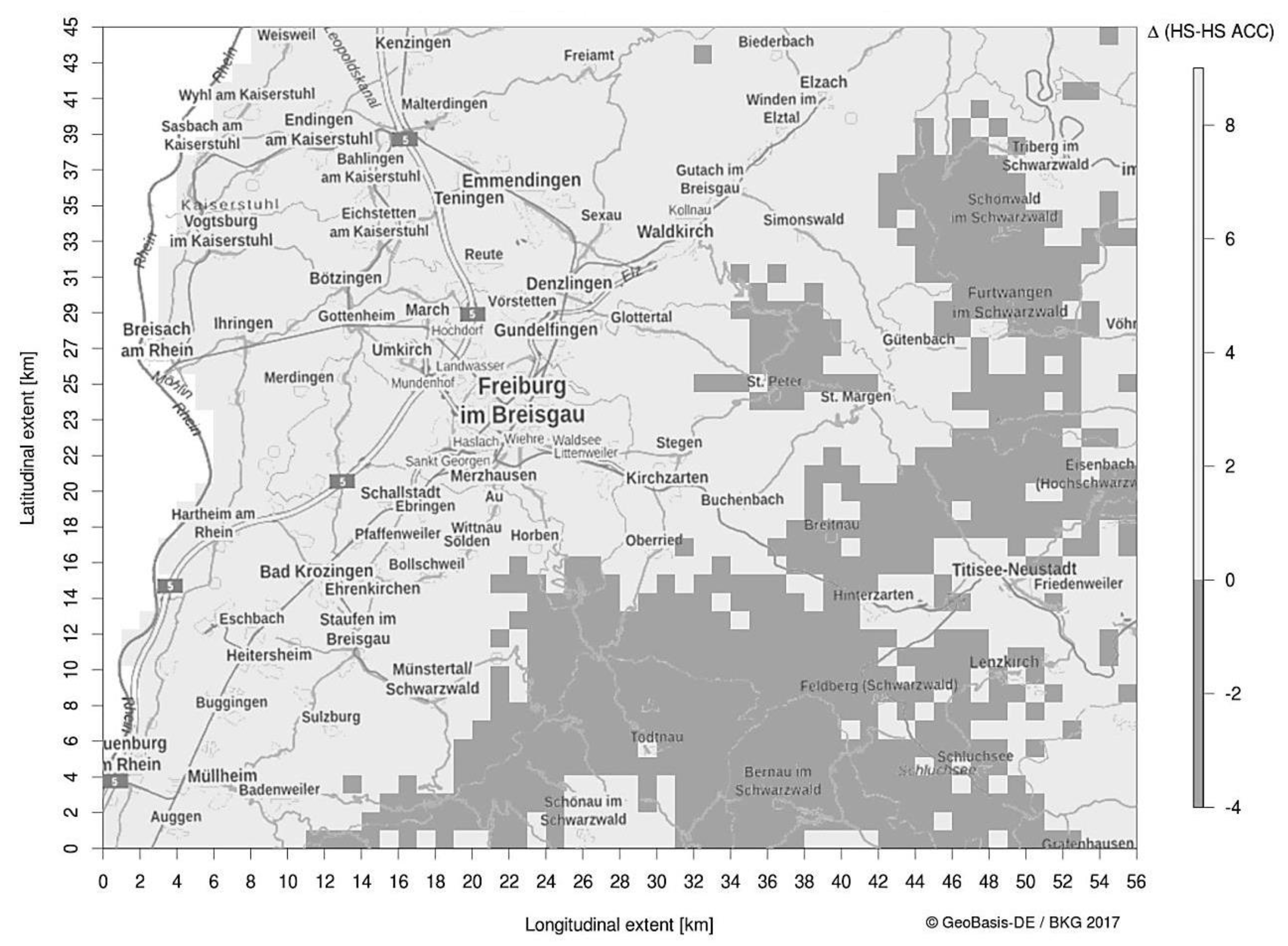
2.2.2. Identifying Days with Heat Stress and Cold Stimulus

Specific thermal conditions and how these conditions affect humans can be defined differently. For this tool, the definition of a day with heat stress (HS day) and cold stimulus (CS day) is taken according to [43] with fixed threshold values (

Table 2. Criteria of calculating days with heat stress or cold stimulus, both with constant and variable threshold values. TH, threshold value; THH, threshold value to heat stress; THC, threshold value to cold stimulus; CET, Central European Time.

Criteria	Heat Stress	Cold Stimulus
Time of analysis	13 CET	7–19 CET
Constant threshold values	THH = 20 °C	THC = 0 °C
Condition with constant TH	PT ≥ THH + 12 °C = 32 °C PT ≥ THH + 6 °C = 26 °C plus sultriness	PT ≤ THC − 6.5 °C = −6.5 °C
Variable threshold values	12 ≤ THH ≤ 22 °C	−4 ≤ THC ≤ 7 °C
Condition with acclimatisation	PT ≥ THH + 12 °C 24 ≤ THH ≤ 34 °C PT ≥ THH + 6 °C 18 ≤ THH ≤ 28 °C plus sultriness	PT ≤ THC − 6.5 °C −10.5 ≤ THC ≤ 0.5 °C

). The threshold values are based on a range of thermal comfort of the Perceived Temperature between 0 °C and 20 °C. Therefore, the threshold value of a day with strong heat stress is defined as the upper boundary of the thermal comfort (20 °C) plus the difference on the class of strong heat stress of 12 °C (20 °C + 12 °C = 32 °C). The definition of a day with cold stimulus is equivalent to this: The lower boundary of thermal comfort minus half of the difference to the physiological class of slight cold stress (0 °C−6.5 °C = −6.5 °C). To identify heat stress, only the Perceived Temperature of 13 CET (Central European Time) is considered, and when checking for cold stimulus, the mean of PT between 7 and 19 CET is considered. This time period comprises the time that (health) tourists are most probably exposed to relevant thermal conditions outdoors. A further definition of heat stress considers the effect of sultriness on the thermal perception. Therefore, a day is also counted as a day with heat stress if PT_{13 CET} ≥ 26 °C (the threshold for moderate heat stress) with simultaneously appearing sultriness.

To consider the effect of short-term acclimatisation within the thermal assessment procedure, the HeRATE (Health Related Assessment of the Thermal Environment) approach, according to [44], is implemented. This approach is assigned to calculate variable threshold values of heat stress and cold stimulus. The effect of acclimatisation shifts the zone of thermal comfort (normal range between 0 °C–20 °C PT) to colder or warmer conditions depending on the thermal conditions of the preceding 30 days. The calculation method of the variable threshold values for the Day of Interest (DOI) is divided into the fixed and the mutable part of the threshold value. The threshold value for heat stress TH_H consists of the fixed part (20 °C PT), counted by two thirds, and the mutable part, which is calculated with the sum of the PT of the preceding 30 days (PT_(D-29:D)) and the Gaussian coefficients (gco), and is counted by one third (Equation (1)). The variable threshold value of heat stress ranges is now, with acclimatisation considered, between approximately 12 °C and fixed 22 °C. The upper boundary is fixed by 22 °C due to the limited ability of the human body to adapt to greater heat. The threshold value for the category “strong heat stress” ranges, therefore, between 24 °C and 34 °C PT (TH_H + 12 °C):

$$\mathrm{THH}\left(\mathrm{DOI}\right)=\frac{2\ast 20}{3}+ \frac{\frac{\sum \left(\mathrm{PT}\left(\mathrm{DOI}-29:\mathrm{DOI}\right)\times \mathrm{gco}\right)}{\sum gco}}{3}.$$

(1)

The same method is applied for the calculation of the threshold value for cold stimulus TH_C (Equation (2)). Here, the fixed part is 0 °C PT. The variable TH_C ranges are now between fixed −4 °C PT and approximately +7 °C PT; the fixed lower boundary is also due to the limited ability of acclimatisation. Considering the effect of acclimatisation, the threshold value for the category “cold stimulus” ranges between approximately −10.5 °C and 0.5 °C PT (TH_C − 6.5 °C):

$$\mathrm{THC}\left(\mathrm{DOI}\right)=\frac{\frac{\sum \left(\mathrm{PT}\left(\mathrm{DOI}-29:\mathrm{DOI}\right)\times \mathrm{gco}\right)}{\sum gco}}{3}.$$

(2)

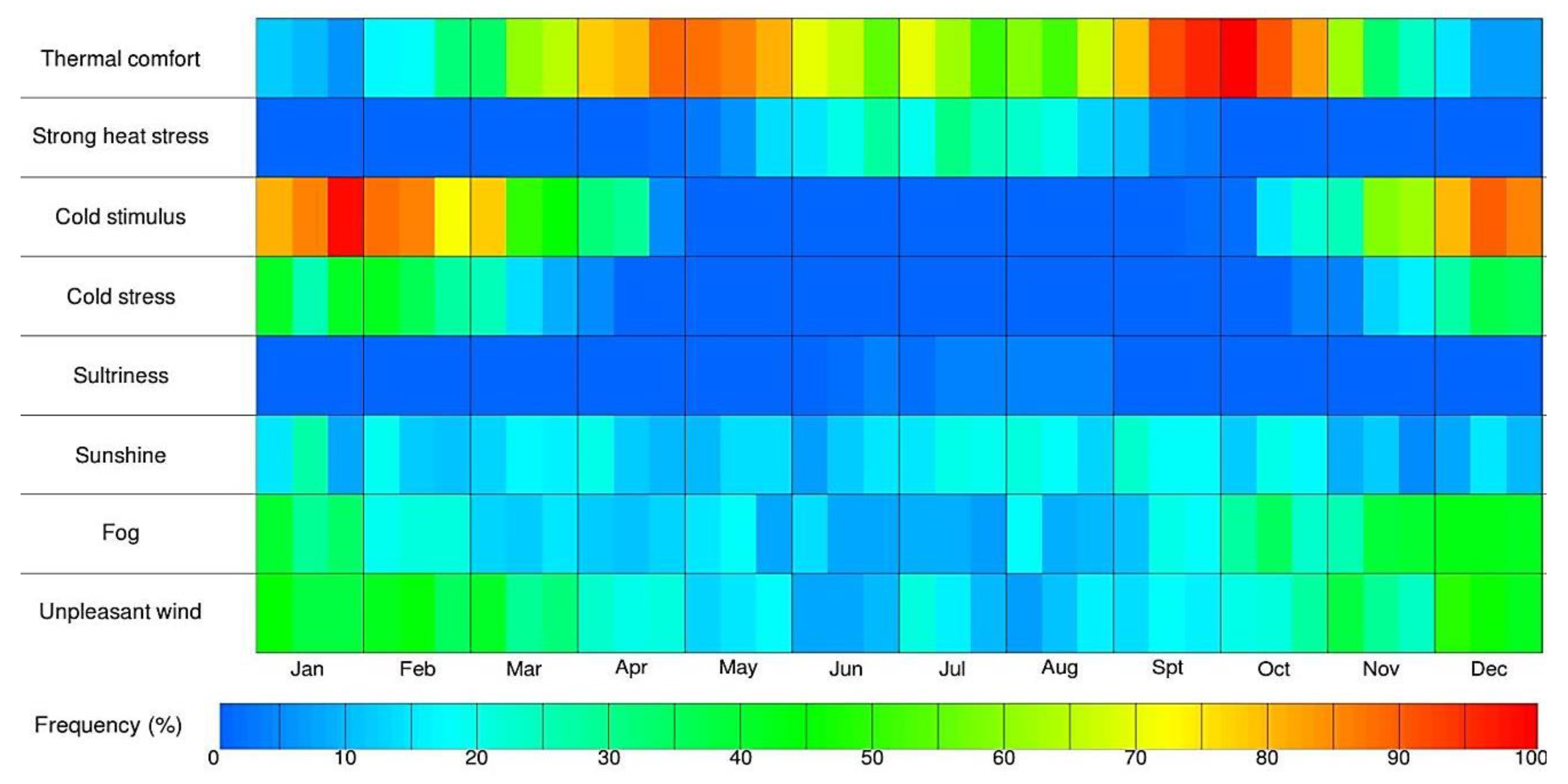
2.2.3. Climate-Tourism/Transfer-Information-Scheme

The Climate-Tourism/Transfer-Information-Scheme (CTIS) depicts the frequency of specific thermal conditions and other meteorological events for the daytime (7–19 CET) [21,22]. The threshold values, from which a day is counted as, for example, a day with thermal comfort, sultriness, or unpleasant wind are different (

Table 3. Method applied to derive the Climate-Tourism-Information-Scheme.

Condition	Threshold Value	Time of Analysis	Minimum Length
Thermal comfort	0 °C ≤ PT ≤ 2 °C	7–19 CET	≥8 h/12 h
Strong heat stress	PT ≥ 32 °C	7–19 CET	≥3 h/12 h
Cold stimulus	PT ≤ −6.5 °C	7–19 CET	≥1 h/12 h
Cold stress	PT ≤ −13 °C	7–19 CET	≥1 h/12 h
Sultriness	d_std ≥ 1	0–23 CET	≥1 h/24 h
Sunshine	CC < 5/8	7–19 CET	12 h/12 h
Fog	RH > 98%	7–19 CET	≥1 h/12 h
Unpleasant wind	v10 > 8 m/s	7–19 CET	≥1 h/12 h

).

To designate a day with thermal comfort, the conditions for this thermal perception have to be present for a minimum of eight hours during the analysis time period from 7–19 CET. If the cloud cover is lower than 5/8 within all twelve hours, the day is declared a day with sunshine. Sultriness is counted during all 24 h due to the loading effect on both day and night, which should appear at least for one hour in order to be counted. Heat stress is counted with a minimum of three hours; cold stimulus, cold stress, fog, and storm are counted from an occurrence of at least one hour during the day.

2.3. Study Area

The study area of southern Baden comprises the city of Freiburg surrounded by the Upper Rhine valley and the German-French border in the west and the Black Forest in the east and south (N 47.777°–N 48.207°, E 7.543°–E 8.297°). The highest mountain of the Black Forest, the Feldberg (south-east from Freiburg), is 1493 m high and with this, is the highest mountain of Germany beyond the Alps. Several health resorts are located in this region of the Black Forest. The largest are the villages Titisee and Hinterzarten, north-east of Feldberg. The altitudes of the study area range from 164 m a.s.l. in the top-left corner of the map to 1458 m a.s.l., averaged in the grid cell of Feldberg. This study area, with an expanse of 56 × 45 km, was chosen due to this great difference in altitude on a relatively small area, displaying the dependence of thermal conditions on height and the effect of acclimatisation. Furthermore, it demonstrates the loading situation of Freiburg and the Upper Rhine Valley compared to the recreational potential of the Black Forest.

3. Results

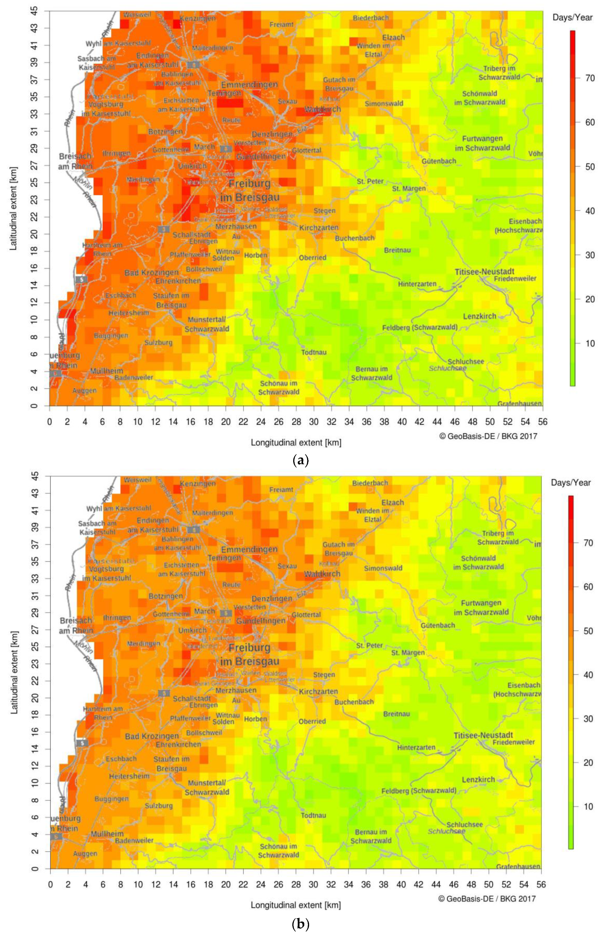
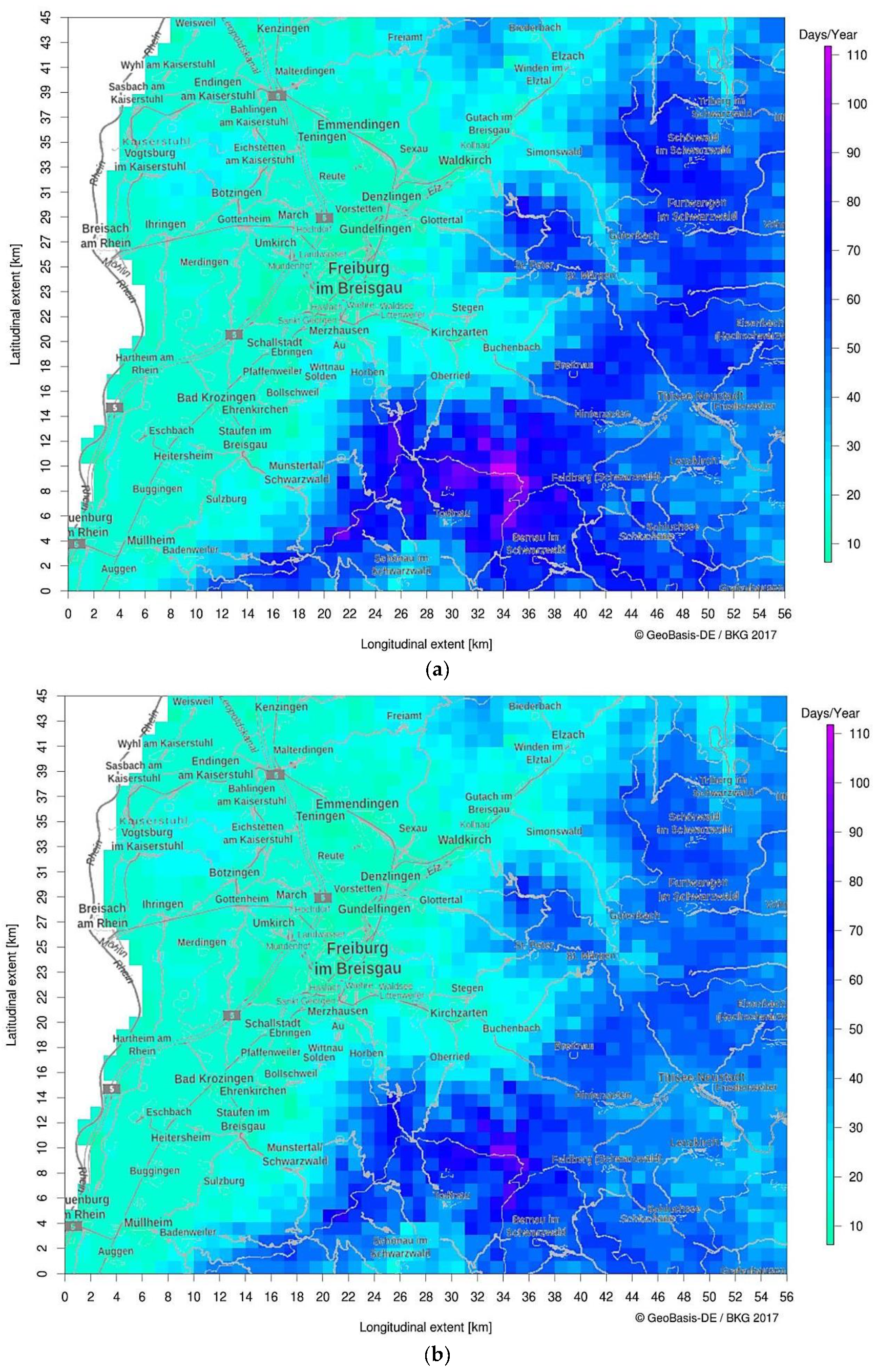
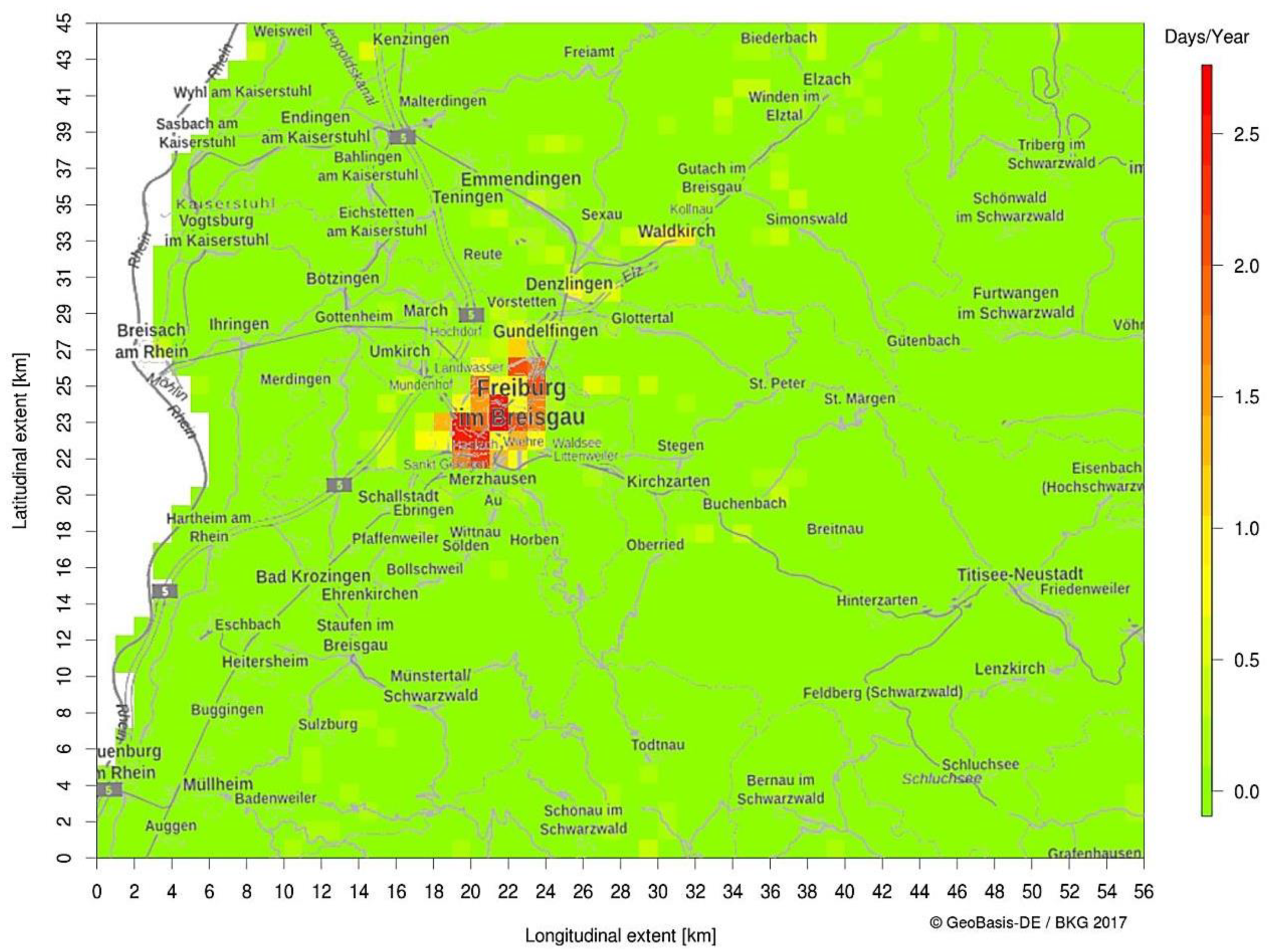
3.1. Study Area of Southern Baden

The area around Freiburg has the lowest number of days with cold stimulus (mean = 13 days) of the study area, with an ascending gradient upstream the river Dreisam towards the Black Forest (Figure 2a). Within the city, the Urban Heat Island effect contributes to higher thermal perception. The low mountain range Kaiserstuhl in the north of Breisach depicts a higher number of days with cold stimulus due to the elevation. The most days with cold stimulus, up to 110 days, occur at Feldberg.

By considering acclimatisation to the thermal condition of the last 30 days, the number of days with cold stimulus (CS_ACC days) is reduced by 5.6 days, averaged over this study area and over the time period from 1995 to 2012 (Figure 2b). However, the range of this difference is very high due to variations in of altitude and climate conditions. The higher the altitude, the more days are reduced by acclimatisation. At Feldberg, the mean number is reduced by 24 days, thereby amounting to only 86 days per year.

On the contrary, the acclimatisation effect increases the number of days with cold stimulus in some areas by a maximum of two days. The days with cold stimulus are important for health resorts located in this region to offer activities, like hiking, which promote fitness. However, acclimatisation mostly affects the residents and visitors only after a longer stay in this region.

The spatial distribution of days with heat stress is likewise noticeable (Figure 3). The number of days with heat stress (HS days) ranges from 3 to 78 days, and the fewest examples of heat stress occur at Feldberg. In the city of Freiburg itself, heat stress occurs an average of 56 days per year. In Hinterzarten, 14 days with heat stress are counted. Within the distance between Freiburg and Hinterzarten, heat stress is reduced by 42 days. If the effect of acclimatisation is considered, the number of days with heat stress (HS_ACC days) decreases by 2.1 days per year averaged over the study area and time period. The maximum decrease amounts to 8.0 days north of Freiburg, and the maximum increase of heat stress with 2.5 days per year occurs at Feldberg.

The spatial distribution of heat stress and cold stimulus draws a well recognisable line between the higher altitude and colder climate of the Black Forest in the east and south of the study area and the lower altitude, with the warmer region of the Rhine Valley in the north and west. The effect of acclimatisation displays the differences in altitude and climate, as well (Figure 4). The mean difference between the number of HS days calculated with the constant threshold value and the number of HS days calculated with the variable threshold value, considering acclimatisation effects (HS_ACC days), illustrates the opposing effect of acclimatisation in warmer and colder regions. While the acclimatisation effect in warmer regions leads to a reduction of days with heat stress (light grey areas), the number of days with heat stress increases in colder regions like the Black Forest (dark grey areas). This is caused by the variable threshold value considering the thermal conditions of the last 30 days.

If these thermal conditions are cooler, the variable threshold value for heat stress decreases. This can lead to the situation that a day with a PT_{13 CET} lower than 32 °C PT is counted as a day with heat stress. The equivalent effect of acclimatisation is also recognisable in the distribution of CS days compared to CS_ACC days, leading to an increase in CS days in the warmer regions near Freiburg and the Rhine Valley and a decrease of CS days in the Black Forest, caused by the different thermal conditions affecting acclimatisation (data not shown).

The thermal conditions at night clearly display the effect of the UHI in Freiburg (Figure 5). Warm nights with a T_{a, min 18-6 CET} ≥ 14 °C occur mainly within the city. The maximum of 2.6 days per year is located in the city centre. Tropical nights with T_{a,min 18-6 CET} ≥ 20 °C appear very rarely throughout the study area, even in the city centre.

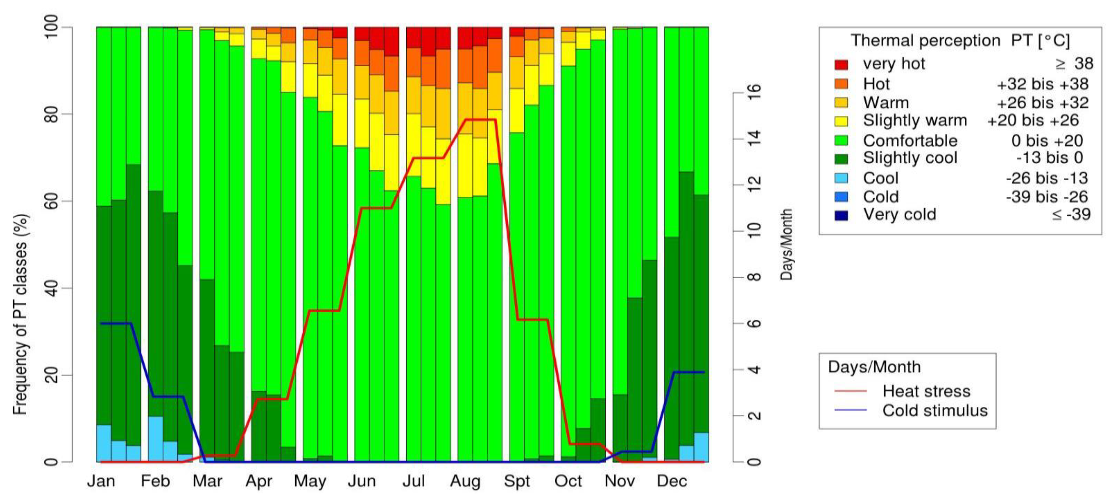
3.2. Comparision of Freiburg with a Health Resort in the Black Forest

Freiburg is an important touristic destination for Germans and, due to its proximity to France and Switzerland, also for French and Swiss visitors. It is one of the biggest cities close to the Black Forest and is ideal for day trips into the mountains. The frequency diagram (Figure 6) and the CTIS of Freiburg (Figure 7) display the climatic conditions of the city. The frequency diagram depicts the annual thermal condition averaged over all available data, i.e., daytime and night-time. In contrast, most parameters displayed in CTIS depict only the daytime conditions. This is the reason for the differences of frequencies in Figure 6 and Figure 7.

Thermal comfort conditions occur throughout the year, in winter with a frequency of approximately 40%, while a minimum frequency of 16% occurs in summer, particularly from late July until mid-August (Figure 7). The high number of days with heat stress during summer (max. 47%) and the presence of sultriness from June to early September (max. 38%) explain this minimum of thermal comfort in summer. Cold stimulus occurs in winter months on up to 52% of days, while cold stress has a maximum frequency of 17%. Days with sunshine have a mean frequency of 16%, with a maximum in late July and a minimum in late November. Fog arises mainly in autumn on up to 22% of days in mid-October. Stormy days are present from December until March, with a mean frequency of 14%.

HS days counted in Freiburg appear frequently in the context of a heat wave, i.e., they are consecutive over a minimum of three days (Figure 8a). Heat waves with more than 15 consecutive days appeared in the years 2003, 2005, 2006, 2009, and 2010. The mean percentage of HS days in the context of a heat wave amounts 44.5% of 55.5 HS days averaged over the time period. Due to the acclimatisation effect, heat waves are less frequent and shorter; of the averaged 49.5, HS_ACC days occur approximately 45% of the time in the context of a heat wave (Figure 8b).

In contrast to the warm climate of Freiburg, Hinterzarten, located at 901 m a.s.l., has different climatic conditions (Figure 9). Hinterzarten, the lake, and the village of Titisee are very well known touristic destinations, but they are known as health resorts too. In general, the Black Forest is used as escape from the loading thermal conditions in Freiburg and the Rhine Valley during summer and for winter sport activities in winter. In Hinterzarten, the two local maxima of thermal comfort in spring and autumn are extended and shifted towards summer.

The mean occurrence of thermal comfort amounts to 50%. From late April until early June, the first maximum of 80% appears, and from September until October, the second maximum of 90% emerges. In-between, the summerly minimum of 46% occurs in early August. This highlights the difference to Freiburg, which has a summerly minimum of 16%. As expected, heat stress occurs only in the summer months with a frequency of up to 27%. However, days with cold stimulus are counted from mid-October until mid-April, with high frequencies up to 89%.

The warm days in summer are mostly accompanied by dry air, and sultriness occurs only on very few days. Days with sunshine occur consistently throughout the year, with a mean frequency of 13%. Fog and storms arise mainly in winter, but both can also occur throughout the year with a higher frequency compared to Freiburg.

3.3. Comparison of Results with a Bioclimatic Map of DWD

The generated heat stress and cold stimulus maps, considering the acclimatisation effect, were compared with the bioclimatic map 1981–2010 of the DWD regarding acclimatisation as well (bioclimatic maps are accessible on DWD website [45]). In general, the number of days with heat stress, identified with the presented data and method for acclimatisation effects, is higher in this study area. However, the same applies to the number of days with a cold stimulus. Differences are induced by meteorological data and the methods used to calculate PT for the bioclimatic map. For the previous bioclimatic map, PT is calculated only with data of the synoptic stations of the DWD. Subsequently, PT is statistically interpolated to generate a meso-scale map with a spatial resolution of 1 km², smoothing colder and warmer conditions. Due to the high resolution of the basic TRY data, extreme values are better represented.

The disadvantage of the basic TRY dataset is that it features the short time period compared to the bioclimatic maps that are available for different standard reference periods. This shorter time period is also an explanation for the more extreme numbers of days with heat stress and cold stimulus. This is observable in Hinterzarten, with a mean of 21 HS days per year, which can be more than the allowed number for a climatic health resort (depending on the thermal conditions during the nights between the heat stress days). Due to the shorter time period, the threshold values for heat stress days in health resorts are only applicable to a limited extend.

4. Discussion

4.1. Appropriate Preparation and Assessment of Climate Data

The basic TRY dataset is statistically generated with meteorological data from synoptic stations, satellite data, and data from a regional climate model. The application possibilities of this dataset are determined by the consistency of data across variables and in time. As the data was generated, the focus was on the consistency between meteorological variables and on short-term temporal consistency over one day. The high spatial resolution requires the utilisation of all available station data fulfilling basic quality [25,46]. However, as the station network changed during the time period from 1995 to 2012, inhomogeneities occurred and limited the consistency in time. This has led to limited capabilities for climatological analyses, such as the identification of long-term trends. The variations in the network density can also demonstrate artificial trends, even in interpolated datasets with a focus on a high temporal consistency [46]. Therefore, interpretation of trends should be done carefully. The consistency across variables and temporally over one day is conformed since it is an essential requirement of the originally data application as Test-Reference-Years [25]. Another limiting factor of climatological analyses is the total length of the data series. Usually, the climatological time scale is 30 years (standard reference period), but the time period of the described dataset is yet only 18 years. Therefore, climatological studies are not yet recommended [25,46]. The DWD extends this dataset gradually for the latest years, and an update of the dataset comprising years up to 2015 will be available soon.

A spatial resolution of at least 1 km² is required to generate high resolution maps, allowing one to evaluate the spatial distribution of climatological parameters over a specific region. Understanding the difficulties in estimating radiation and wind speed, and the low density of station measurements for radiation components, it is evident that the gridded dataset cannot capture all variations of the parameters that may occur within the 1 km² resolution. This also applies to the other meteorological variables in the complex terrain. Further, it should be noted that over-smoothing (smoothing out of extreme values, induced by the kriging and spline interpolation) is quite possible in datasets with spatial interpolation [47]. This over-smoothing leads to an under-estimation of high percentiles and an over-estimation of lower percentiles [25]. Therefore, the results for POI have to be interpreted with this knowledge. The temporal resolution of one hour is necessary to display the diurnal distribution of (bio-)climatic parameters and to reveal loading conditions like heat stress around noon. Today, a measurement interval of at least one hour is standard of synoptic station.

4.2. Assessment of Human-Biometeorological Methods

The Perceived Temperature was chosen as one of several possible thermal indices due to its comparability to the bioclimatic map of the DWD and other studies using this index in Germany. Other indices like PET or UTCI are applicable as well. In this tool, calculating thermal index and threshold values for heat stress and cold stimulus have to be adapted. The uncertainty of PT is conditioned by the insecurity of the individual input parameters T_a, VP, v_1.1, and T_mrt.

The HeRATE approach was implemented to consider human acclimatisation to the thermal environment. This modifies the number of days with heat stress and cold stimulus identified in other studies, as well as in the previous bioclimatic maps of the DWD and in the climatic report for health resorts. Therefore, the threshold values, e.g., for days with heat stress allowed in a health resort, have to be modified, in order to adjust to the new method. By considering acclimatisation, the thermal perception of people living permanently with the local climate is estimated. Newly arrived guests of a health resort have to acclimatise initially to the local climate, so thermal perception can deviate from that of the locals and also from the perception estimated by the HeRATE approach [44].

The analysis of the variable threshold values for heat stress and cold stimulus derived with the HeRATE approach depicts an annual variation with a range of approximately 10 °C, from 12 °C to 22 °C for TH_H, and from −4 °C to 7 °C for TH_C. Despite the low TH_H during winter, days with heat stress occur only between May and October (data not shown). Days with cold stimulus, identified with the variable threshold value TH_C, occur between October and April, despite the positive TH_C during summer. Therefore, there is no need to limit the threshold values additionally to the already existing limits. The overlapping of days with heat stress and cold stimulus is induced by the large study area of southern Baden with highly different thermal conditions. Hence, additional days with heat stress and cold stimulus due to acclimatisation occur for some regions within their expected range [48].

4.3. Appropriate Visualisation of Results

Considering the different ways to visualise POI data for tourism and health resorts, a frequency distribution diagram and CTIS diagram were chosen. The frequency distribution of PT classes represents the different thermal conditions of the selected POI as a mean annual or diurnal distribution. Additional to the frequency diagrams displaying only thermal components, the CTIS also represents meteorological parameters like wind speed, cloud cover, and the occurrence of fog. The CTIS diagram, as an objective depiction of data, is more detailed compared to a single value of a tourism climate index. The user gets the frequency distribution of different meteorological and human biometeorological parameters and can identify periods with suitable climatic conditions for his vacation. Citizens can get an overview of climatic conditions within the (favoured) residential area. Therefore, the CTIS is appropriate for all possible user groups, not only for tourists, which is the reason for the inclusion of “Transfer” in the name of CTIS [33]). The variance of the parameters within months justifies and confirms the temporal resolution of an approximately ten day period.

The maps of AOI display the occurrence and spatial distribution of extreme or health-relevant events. This representation of spatial distributed data can be much more helpful as information for a POI, e.g., for a choice of location for a holiday or a new residence. This is possible only with gridded data. The spatial resolution of 1 km² is suitable for several purposes and application, e.g., as a climatic map of a city and its surroundings, to compare districts, and as an overview of a touristic region to select the best location for a vacation.

The tool providing different maps can also be seen as interactive version of the bioclimatic map of the DWD, with additional features like the displayed acclimatisation effect, nightly heat stress, and additional information of a chosen POI.

5. Conclusions

The tool was developed to generate human bioclimatic information about the temporal and spatial distribution of heat stress, cold stimulus, thermal comfortable conditions, and the occurrence of heat waves. This information is represented with different diagrams and maps trying to meet the requirements of all possible user groups. Therefore, this tool offers an additional value for the field of human-biometeorology.

The calculations, analyses and results of this study reveal that the appropriate preparation and assessment of data, biometeorological methods, and visualisation are strongly dependent on the data available. The basic TRY dataset does not allow the analysis or depiction of climatological trends or single years. These values have to be considered by the assessment of bioclimatic information and by the visualisation of this information. The preparation of climatic data for human biometeorological methods should be consequent for all parameters required; otherwise, the differences and their consequences have to be noted. All data and information used to generate a human thermal index contribute to the insecurity of the resulting parameter. A spatial resolution of 1 km² is needed for a meso-scaled map, but the interpolation methods, additional data sources, and models can lead to differences in which meteorological phenomena occurring within a grid cell are considered. A temporal resolution of at least one hour is essential to depict the diurnal distribution of parameters and to identify health-related thermal conditions, like heat stress.

Short-term acclimatisation is considered by the assessment of meteorological and physiological conditions relevant to the thermal perception of humans. This affects the number of days with heat stress and other thermal conditions and is only relevant for residents of the study area. Tourists and visitors have to acclimatise to the local climate of the destination (if this differs from their usual climate) before they can adapt to a current event like a heat wave. Therefore, and because of its comparability and comprehensibility, heat stress calculated with both methods is represented. The adverse effect of acclimatisation on the number of days with heat stress in colder and warmer regions has to be considered, e.g., by analysing climate health resorts. The advantage of this gridded data is the possibility to analyse spatial distributions of parameters and, therefore, examine the surroundings of, e.g., a health resort.

A tool with free access for the public is not yet implemented on the website of the DWD. The design of the website and input form, linking to the other offers of the DWD, and suitable promotion of this tool are the next steps of this project. The diagrams and maps have to be accompanied by explanations to ensure an appropriate evaluation of the results.

Despite these restrictions, this tool enriches the human-biometeorological offerings of the DWD and can offer information valuable to different users and for different applications in several economic sectors.

References

1. Jendritzky, G. The atmospheric environment—An introduction. Experientia 1993, 49, 733–740. [Google Scholar] [CrossRef]
2. Basu, R.; Samet, J.M. Relation between elevated ambient temperature and mortality: A review of the epidemiologic evidence. J. Epidemiol. Rev. 2002, 24, 190–202. [Google Scholar] [CrossRef]
3. Parsons, K. Human Thermal Environments: The Effects of Hot, Moderate, and Cold Environments on Human Health, Comfort, and Performance; CRC Press: Boca Raton, FA, USA, 2014. [Google Scholar]
4. Staiger, H.; Laschewski, G.; Matzarakis, A. Selection of Appropriate Thermal Indices for Applications in Human Biometeorological Studies. Atmosphere 2019, 10, 18. [Google Scholar] [CrossRef]
5. Jendritzky, G.; Menz, G.; Schmidt-Kessen, W.; Schirmer, H. Methodik der räumlichen Bewertung der thermischen Komponente im Bioklima des Menschen (Fortgeschriebenes Klima-Michel-Modell); Beiträge der Akademie für Raumforschung und Landesplanung: Hannover, Germany, 1990. [Google Scholar]
6. Staiger, H.; Bucher, K.; Jendritzky, G. Gefühlte Temperatur. Die physiologisch gerechte Bewertung von Wärmebelastung und Kältestress beim Aufenthalt im Freien in der Maßzahl Grad Celsius. Annalen der Meteorologie 1997, 33, 100–107. [Google Scholar]
7. Staiger, H.; Laschewski, G.; Grätz, A. The perceived temperature—A versatile index for the assessment of the human thermal environment. Part A: Scientific basics. Int. J. Biometeorol. 2012, 56, 165–176. [Google Scholar] [CrossRef]
8. Mayer, H.; Höppe, P. Thermal comfort of man in different urban environments. Theor. Appl. Climatol. 1987, 38, 43–49. [Google Scholar] [CrossRef]
9. VDI. Environmental Meteorology, Methods for the Human Biometeorological Evaluation of Climate and Air Quality for the Urban and Regional Planning at Regional Level; VDI: Berlin, Germany, 1998; Volume 3787. [Google Scholar]
10. Höppe, P. The physiological equivalent temperature—A universal index for the biometeorological assessment of the thermal environment. Int. J. Biometeorol. 1999, 43, 71–75. [Google Scholar] [CrossRef]
11. Matzarakis, A.; Mayer, H.; Iziomon, M.G. Applications of a universal thermal index: Physiological equivalent temperature. Int. J. Biometeorol. 1999, 43, 76–84. [Google Scholar] [CrossRef]
12. Jendritzky, G.; de Dear, R.; Havenith, G. UTCI—Why another thermal index? Int. J. Biometeorol. 2012, 56, 421–428. [Google Scholar] [CrossRef]
13. Hensel, H. Temperaturreglation. In Kurzgefasstes Lehrbuch der Physiologie; Keidel, W.D., Ed.; Thieme-Verlag: Stuttgart, Germany, 1973; pp. 224–235. [Google Scholar]
14. Koppe, C. Gesundheitsrelevante Bewertung von thermischer Belastung unter Berücksichtigung der kurzfristigen Anpassung der Bevölkerung an die lokalen Witterungsverhältnisse; Deutschen Wetterdienstes: Offenbach, Germany, 2005. [Google Scholar]
15. ASHRAE. The 2005 Handbook: Fundamentals; American Society of Heating, Refrigerating and Air-Conditioning Engineers Inc.: Atlanta, GA, USA, 2005. [Google Scholar]
16. Matzarakis, A. Das Hitzewarnsystem des Deutschen Wetterdienstes (DWD) und seine Relevanz für die menschliche Gesundheit. Gefahrstoffe-Reinhaltung der Luft 2016, 76, 457–460. [Google Scholar]
17. Armstrong, L.E. Heat acclimatization. In Encyclopedia of Sports Medicine and Science; Internet Society for Sport Science (Hrsg.: Fathey, D.B.): Reston, VA, USA, 1998. [Google Scholar]
18. Matzarakis, A. Weather and climate-related information for tourism. Tour. Hospitality Plan. Dev. 2006, 3, 99–4115. [Google Scholar] [CrossRef]
19. de Freitas, C.R. Tourism climatology: Evaluating environmental information for decision making and business planning in the recreation and tourism sector. Int. J. Biometeorol. 2003, 48, 45–454. [Google Scholar] [CrossRef]
20. Becker, P.; Bucher, K.; Grätz, A.; Koppe, C.; Laschewski, G. Das medizin-meteorologische Informationsangebot für den Gesundheitssektor und die Öffentlichkeit. Promet. 2007, 33, 140–147. [Google Scholar]
21. Matzarakis, A. Assessment method for climate and tourism based on daily data. Dev. Tour. Climatol. 2007, 52–58. [Google Scholar]
22. Lin, T.P.; Matzarakis, A. Tourism climate and thermal comfort in Sun Moon Lake, Taiwan. Int. J. Biometeorol. 2008, 52, 281–290. [Google Scholar] [CrossRef]
23. Ebi, K.L.; Schmier, J.K. A stitch in time: Improving public health early warning systems for extreme weather events. Int. J. Biometeorol. 2005, 27, 115–121. [Google Scholar] [CrossRef]
24. Stocker, T. Climate Change 2013: The Physical Science Basis: Working Group I Contribution to the Fifth Assessment Report of the Intergovernmental Panel on Climate Change; Cambridge University Press: Cambridge, UK, 2014. [Google Scholar]
25. Krähenmann, S.; Walter, A.; Brienen, S.; Imbery, F.; Matzarakis, A. High-resolution grids of hourly meteorological variables for Germany. Theor. Appl. Climatol. 2018, 131, 899–926. [Google Scholar] [CrossRef]
26. Böhm, U.; Kücken, M.; Ahrens, W.; Block, A.; Hauffe, D.; Keuler, K.; Rockel, B.; Will, A. CLM—The climate version of LM: Brief description and long-term applications. COSMO Newsletter 2006, 6, 225–235. [Google Scholar]
27. Oke, T.R. The energetic basis of the urban heat island. Q. J. R. Meteor. Soc. 1982, 108, 1–24. [Google Scholar] [CrossRef]
28. Rizwan, A.M.; Dennis, L.Y.C.; Chunho, L. A review on the generation, determination and mitigation of Urban Heat Island. J. Environ. Sci. 2008, 20, 120–128. [Google Scholar] [CrossRef]
29. Oke, T. Boundary Layer Climates, 2nd ed.; Methuen Co.: London, UK, 1987. [Google Scholar]
30. Mayer, H.; Matzarakis, A.; Iziomon, M.G. Spatio-temporal variability of moisture conditions within the Urban Canopy Layer. Theor. Appl. Climatol. 2003, 76, 165–179. [Google Scholar] [CrossRef]
31. Kuttler, W.; Weber, S.; Schonnefeld, J.; Hesselschwerdt, A. Urban/rural atmospheric water vapour pressure differences and urban moisture excess in Krefeld, Germany. Int. J. Climatol. 2007, 27, 2005–2015. [Google Scholar] [CrossRef]
32. DWD. Climate Data Center FTP-Server. Available online: ftp://ftp-cdc.dwd.de/pub/CDC/grids_germany/hourly/Project_TRY/ (accessed on 20 March 2019).
33. Matzarakis, A. Transfer of climate data for tourism applications—The climate-tourism/transfer-information-scheme. Sustain. Environ. Res. 2014, 24, 273–280. [Google Scholar]
34. Zaninović, K.; Matzarakis, A. The bioclimatological leaflet as a means conveying climatological information to tourists and the tourism industry. Int. J. Biometeorol. 2009, 53, 369–374. [Google Scholar] [CrossRef]
35. Matzarakis, A.; Rutz, F.; Mayer, H. Modelling radiation fluxes in simple and complex environments—Application of the RayMan model. Int. J. Biometeorol. 2007, 51, 323–334. [Google Scholar] [CrossRef]
36. Matzarakis, A.; Rutz, F.; Mayer, H. Modelling radiation fluxes in simple and complex environments: Basics of the RayMan model. Int. J. Biometeorol. 2010, 54, 131–139. [Google Scholar] [CrossRef]
37. Kuttler, W. Stadtklima. In Handbuch der Umweltveränderungen und Ökotoxologie; Guderian, R., Ed.; Springer: Berlin, Germany, 2000; Vol. Band 1B Atmosphäre, pp. 420–470. [Google Scholar]
38. Matzarakis, A.; De Rocco, M.; Najjar, G. Thermal bioclimate in Strasbourg-the 2003 heat wave. Theor. Appl. Climatol. 2009, 98, 209–220. [Google Scholar] [CrossRef]
39. Fanger, P.O. Thermal Comfort, Analysis and Application in Environmental Engineering; DANISH TECHNICAL PRESS: Copenhagen, Denmark, 1972. [Google Scholar]
40. VDI. Environmental Meteorology, Methods for the Human-Biometeorological Evaluation of Climate and Air Quality for the Urban and Regional Planning at Regional Level; VDI: Berlin, Germany, 2008; Volume 3787, p. 29. [Google Scholar]
41. Gagge, A.P.; Fobelets, A.P.; Berglund, L.G. A standard predictive Index of human reponse to thermal enviroment. ASHRAE 1986, 92, 709–731. [Google Scholar]
42. Staiger, H.; Laschewski, G.; Matzarakis, A. A short note on the inclusion of sultriness issues in perceived temperature in mild climates. Theor. Appl. Climatol. 2018, 131, 819–826. [Google Scholar] [CrossRef]
43. VDI. Environmental Meteorology—Human Biometeorological Re-Quirements in the Framework of Recreation, Prevention, Therapy and Rehabilitation; VDI: Berlin, Germany, 2010; Volume 3787. [Google Scholar]
44. Koppe, C.; Jendritzky, G. Inclusion of short-term adaptation to thermal stresses in a heat load warning procedure. Meteorol. Z 2005, 14, 271–278. [Google Scholar] [CrossRef]
45. DWD. Bioklimakarte Deutschland (Bioclimatic Map Germany). Available online: https://www.dwd.de/DE/leistungen/bioklimakarte/bioklimakarte.html (accessed on 20 March 2019).
46. Hiebl, J.; Frei, C. Daily temperature grids for Austria since 1961—Concept, creation and applicability. Theor. Appl. Climatol. 2016, 124, 161–178. [Google Scholar] [CrossRef]
47. Haylock, M.R.; Hofstra, N.; Tank, A.M.G.; Klok, E.J.; Jones, P.D.; New, M. A European daily high-resolution gridded data set of surface temperature and precipitation for 1950–2006. J. Geophys. Res. Atmos. 2008, 113. [Google Scholar] [CrossRef]
48. Endler, C.; Oehler, K.; Matzarakis, A. Vertical gradient of climate change and climate tourism conditions in the Black Forest. Int. J. Biometeorol. 2010, 54, 45–61. [Google Scholar] [CrossRef]
Figure 1. The calculations procedure of the tool for a Point or Area of Interest in eight steps. Ta, air temperature; RH, relative humidity; v, wind speed; G, global radiation; CC, cloud cover; Tmrt, mean radiant temperature; PT, Perceived Temperature; CTIS, Climate-Tourism/Transfer-Information-Scheme.
Atmosphere 10 00334 g001
Figure 2. Spatial distribution of cold stimulus within the study area of southern Baden averaged over the time period 1995–2012: (a) cold stimulus days without consideration of acclimatisation effects (CS days) and (b) CS days with acclimatisation effects (CSACC days).
Atmosphere 10 00334 g002
Figure 3. Spatial distribution of heat stress within the study area of southern Baden averaged over the time period 1995–2012: (a) heat stress days without consideration of acclimatisation effects (HS days) and (b) HS days with acclimatisation effects (HSACC days).
Atmosphere 10 00334 g003
Figure 4. Spatial distribution of the mean difference between HS days (heat stress without acclimatisation effect) and HSACC days (heat stress acclimatisation effect) during the time period 1995–2012. Negative differences (dark grey) imply an increase in days with heat stress due to the acclimatisation effect, and positive differences (light grey) imply a decrease in days with heat stress.
Atmosphere 10 00334 g004
Figure 5. Spatial distribution of nightly heat stress expressed with the mean number of warm nights with Ta, min 18-6 CET ≥ 14 °C within the study area of southern Baden over the time period 1995–2012. The calculation was conducted without consideration of acclimatisation effects.
Atmosphere 10 00334 g005
Figure 6. Frequency diagram of the Perceived Temperature of the city of Freiburg, extracted from the area of interest of southern Baden, averaged over the time period 1995–2012 (6–18 UTC).
Atmosphere 10 00334 g006
Figure 7. CTIS of the city of Freiburg, extracted from the AOI of southern Baden, averaged over the time period 1995–2012 (6–18 UTC).
Atmosphere 10 00334 g007
Figure 8. Consecutive number of days with heat stress for Freiburg during the time period 1995–2012: (a) without acclimatisation effects and (b) with acclimatisation effects. Grey bars depict the total number of HS respectively HSACC days of the year.
Atmosphere 10 00334 g008
Figure 9. The CTIS of Hinterzarten, extracted from the AOI of southern Baden, averaged over the time period 1995–2012.
Atmosphere 10 00334 g009