Article

Impacts of Green Vegetation Fraction Derivation Methods on Regional Climate Simulations

by
Jose Manuel Jiménez-Gutiérrez
1,
Francisco Valero
1,
Sonia Jerez
2 and
Juan Pedro Montávez
2,*
1
Departamento de Astrofísica y Ciencias de la Atmósfera, Universidad Complutense de Madrid, 28040 Madrid, Spain
2
Departamento de Física, Universidad de Murcia, 30100 Murcia, Spain
*
Author to whom correspondence should be addressed.
Atmosphere 2019, 10(5), 281; https://doi.org/10.3390/atmos10050281
Submission received: 8 March 2019 / Revised: 13 May 2019 / Accepted: 15 May 2019 / Published: 21 May 2019
(This article belongs to the Special Issue Lower Atmosphere Meteorology)

Abstract

:
The representation of vegetation in land surface models (LSM) is crucial for modeling atmospheric processes in regional climate models (RCMs). Vegetation is characterized by the green fractional vegetation cover (FVC) and/or the leaf area index (LAI) that are obtained from nearest difference vegetation index (NDVI) data. Most regional climate models use a constant FVC for each month and grid cell. In this work, three FVC datasets have been constructed using three methods: ZENG, WETZEL and GUTMAN. These datasets have been implemented in a RCM to explore, through sensitivity experiments over the Iberian Peninsula (IP), the effects of the differences among the FVC data-sets on the near surface temperature (T2m). Firstly, we noted that the selection of the NDVI database is of crucial importance, because there are important bias in mean and variability among them. The comparison between the three methods extracted from the same NDVI database, the global inventory modeling and mapping studies (GIMMS), reveals important differences reaching up to 12% in spatial average and and 35% locally. Such differences depend on the FVC magnitude and type of biome. The methods that use the frequency distribution of NDVI (ZENG and GUTMAN) are more similar, and the differences mainly depends on the land type. The comparison of the RCM experiments exhibits a not negligible effect of the FVC uncertainty on the monthly T2m values. Differences of 30% in FVC can produce bias of 1 C in monthly T2m, although they depend on the time of the year. Therefore, the selection of a certain FVC dataset will introduce bias in T2m and will affect the annual cycle. On the other hand, fixing a FVC database, the use of synchronized FVC instead of climatological values produces differences up to 1 C, that will modify the T2m interannual variability.

1. Introduction

Land surface features play a very important role in modulating surface-atmosphere interactions. This is an overlooked issue in climate simulations [1] and short-term weather forecasting [2]. Surface components like soil moisture, albedo, emissivity, surface roughness, vegetation type and amount are fundamental since they control the energy partition at surface [3]. Therefore, the representation of all these variables in land surface models (LSM) is crucial for modeling atmospheric processes.
Atmosphere and vegetation interact in different ways, controlling evapotranspiration, moisture availability, momentum transfer, partitioning radiation, etc. Vegetation is characterized within numerical weather prediction models (NWPM) and RCMs by FVC, LAI and the vegetation class [4]. Therefore, realistic characterization of these parameters should lead to a better reproduction of atmosphere-surface processes.
Different methodologies have been reported for obtaining FVC and LAI through satellite NDVI data [5,6,7,8]. According to Gutman and Ignatov [6] both parameters should not be used simultaneously in the same parameterization. Therefore, it is necessary to prescribe one of the indices and derive the other. Gutman and Ignatov [6] and Carlson et al. [9] argued that is preferable to derive FVC and prescribe LAI, because the exponential dependence of LAI and NDVI saturates after a certain threshold, becoming LAI insensitive to changes in NDVI. Some other authors [7,10] recommend to derive LAI (fixing FVC), because they assume that spatial and seasonal variations of NDVI are related with variations of LAI and validation of FVC is problematical because of the requirement of information at the scale of individual plant elements. Anyway, Godfrey et al. [2] argue that errors introduced by the dual specification of vegetation parameters from a single NDVI observation are likely smaller than uncertainties associated to initial conditions.
The role of vegetation parameters (FVC and LAI) is relevant for weather forecasting and climate change assessments [11]. Their impact on land surface processes has been studied in the Eta operational model [12,13,14] and the Weather Research and Forecasting model (WRF) [15,16,17,18,19,20]. The relevance of using realistic information of the vegetation state on RCM performance has been analyzed in several works. Meng et al. [21] and Müller et al. [22] study the impact of vegetation in concrete cases of droughts in Australia and South America. Other works investigate the contribution of near real time values of vegetation fraction to simulated precipitation. For instance, vegetation–atmosphere feedback in monsoon systems [23,24], severe convection episodes [25], or improving model performance in oasis-desert systems [26]. Other interesting studies focus on vegetation effects on regional climate simulations in complex urban areas like Los Angeles [27,28].
However, the characterization of vegetation is subjected to several sources of uncertainty. On one hand, there are several NDVI database available for obtaining FVC data. They differ in aspects such as the methods for correcting errors, type of satellite, etc. The differences among these NDVI databases reach, for example, similar values to the observed trends in the phenological phases [29]. On the other hand, several methodologies can be used to obtain FVC or LAI from NDVI data [4,6,13,30]. Crawford et al. [31] points out that differences up to 25% in LAI and FVC can easily occur among the different methodologies, similar values to the FVC interannual variability.
In addition, most of the standard configurations of NWPM and RCM use climatological values of vegetation parameters. However, the vegetation has a strong inter-annual variability [18,21,31], leading this to a non-suitable characterization of surface properties. A known limitation is that surface properties can vary at several time scales depending on climate conditions and other processes such as urbanization, forest fires or changes in crops [32].
As an example of the impact of using different approaches with FVC datasets in a LSM, Miller et al. [30] describe, using the Noah LSM, noteworthy differences in surface fluxes, comparing a five-year climatology data from the Advanced Very High Resolution Radiometer (AVHRR) and NASA’s Moderate Resolution Imaging Spectrometers (MODIS) data from the year 2000. With differences of 25% in FVC in monthly-averaged values for all pixels of dry land and cropland of the same two-degree box, transpiration was modified in 30 W m 2 , latent heat fluxes in 10 W m 2 , and sensible heat fluxes in −20 W m 2 . Other works, where real-time satellite data have been used instead of climatological values, have found improvements in the forecasts of T2m in RCM simulations [13,33]. While other studies, indicates that the model sensitivity is not reliable with improved vegetation parameters [2,15,23], stressing the significance of minimizing errors in surface initial conditions (especially soil moisture) or canopy resistance parameterization.
The objective of this work is to assess the impact on T2m simulated by a RCM, of the uncertainty associated to the use of different NDVI data, different methodologies for obtaining FVC, as well as the temporal variability of surface properties in regional climate simulations. Our work will focus on IP, since it is characterized by a large variety of vegetation classes, with a strong seasonal and interannual climate variability that leads to important changes in the state of vegetation.

2. Methods and Data

2.1. NDVI Data

The NDVI is defined as:
N D V I = N I R V I S N I R + V I S ,
where NIR and VIS are the amounts of near-infrared and red visible, respectively, reflected by the vegetation and captured by the satellite sensor [34]. This index was highly correlated with the photo synthetically active biomass, chlorophyll abundance and energy absorption [35] and has been widely used in studies involving land-biosphere interactions [6,13,30,31,36].
There are several global coarse-resolution satellite spectral vegetation index datasets [37]. For example, Satellite Pour l’Observation de la Terre (SPOT Vegetation) and MODIS datasets which have higher resolution and significant improvements with regard to the 1981–2004 record of the AVHRR dataset. However, the latter is an invaluable and irreplaceable archive of historical land surface information and the most used dataset for deriving NDVI due to its long record. Since 1984 several global land surface NDVI data have been derived from AVHRR, as can be the global vegetation index (GVI) dataset [38,39], the NASA Pathfinder 8-km dataset [40] and the GIMMS-NDVI [37,41]. Other datasets, such as the EFAI-NDVI [29], were derived from the NASA Pathfinder 8 km data. These datasets were corrected by taking into account artifacts from sensors, orbital drifting, atmospheric corrections and cloud screening.
Therefore, NDVI values can vary from a database to another in an remarkable way. The GIMMS-NDVI and EFAI-NDVI datasets were chosen to perform our analysis. The selection was done following criteria of NDVI data already processed, easily/free availability and temporal extension.
The EFAI-NDVI covers the period 1982–2001 and corrects the original AVHRR data to create a continuous dataset of 10-day temporal and 0.1 spatial resolutions with global coverage. The correction method implies a spatial interpolation of missing values and processing artifacts as well as a temporal interpolation of the NDVI series throughout a Fourier adjustment algorithm [10,29].
The GIMMS-NDVI [42] from the AVHRR dataset covers from 1982 to 2006 with a spatial resolution of 8 km. This database has been corrected for calibration, view geometry, volcanic aerosols, and other effects non related to vegetation change. In particular, NOAA-9 descending node data from September 1994 to January 1995, volcanic stratospheric aerosol correction for 1982–1984 and 1991–1994, and improved NDVI using empirical mode decomposition/reconstruction to minimize effects of the orbital drift.

2.2. Deriving FVC from NDVI Data

FVC is defined as the fraction of horizontal area associated with the photosynthetically active green vegetation that occupies a model grid cell [43]. In our experiments we derive FVC and use prescribed LAI, because of our LSM, Noah, considers this option in its configuration.
FVC calculation from NDVI data [44] can be based on linear models [6] or quadratic models [45]. These methods take as reference bare soil ( N D V I 0 ) and dense green vegetation( N D V I ). Such values can be prescribed or estimated from the actual NDVI data. For instance, Montandon and Small [44] studied the impact of varying N D V I 0 , showing how its underestimation yields a FVC overestimation.
In this study, three linear models, WETZEL, GUTMAN and ZENG have been selected as a basis to study the uncertainty in FVC calculation and its impacts on RCMs runs. These methods present different degrees of complexity, being the WETZEL/ZENG method the most simple/complex, while GUTMAN is of intermediate complexity. This latter has been extensively used in generating data for NWPMs.
The three methodologies have been applied to the GIMMS-NDVI data. Monthly FVC values have been calculated from 1982 to 2006 with a spatial resolution of 0.1 .

2.2.1. Wetzel Method

In Chang and Wetzel [5] a two-line-segment method is presented. The slope of the linear relationship between NDVI and FVC changes when NDVI exceeds 0.547. The relation is as follows:
F V C = 1.5 ( N D V I 0.1 ) , N D V I 0.547 3.2 ( N D V I ) 1.08 , N D V I > 0.547 ,
being that the FVC is constrained to be between 0 and 1.
The FVC data obtained by this method is used in the MM5 LSM model by Crawford et al. [31] and in the ETA model by Kurkowski et al. [13].

2.2.2. Gutman Method

This method uses the following simple linear relationship between NDVI and FVC:
F V C = N D V I v a l N D V I 0 N D V I N D V I 0 ,
where N D V I 0 and N D V I are the values for bare soil and dense green vegetation.
Gutman and Ignatov [6] take N D V I 0 = 0.04 and N D V I = 0.52, which correspond respectively to the minimum NDVI value of the desert cluster and the maximum NDVI value of the evergreen cluster in their study with GVI data. These values are in principle, region and season specific, since they depend on the soil and vegetation types and the vegetation chlorophyll content [46]. However, the authors take this assumption because there are many intermediate cases that make the evaluation difficult for other surface types. In this work, N D V I 0 and N D V I , have been set to 0.1 (2% percentile of bare soil) and 0.91 (98% Evergreen vegetation) using the GIMMS-NDVI database.

2.2.3. Zeng Method

This method includes procedures that involve the analysis of NDVI data as a function of biome or land cover type. This approach has been used in several works [7,15,30,43]. It follows the simple relationship between FVC and NDVI described by Gutman and Ignatov [6] (Equation (3)). The values of N D V I are calculated analyzing the frequency distribution of maximum NDVI for each land cover type.
This study uses the University of Maryland Department (UMD) global land cover classification [47,48]. This land cover database has been chosen because it was created using the same NDVI data as the GIMMS-NDVI database. Figure 1a (forest types) and Figure 2a (shrubland, cropland and grassland) show the spatial distribution as well as the relative frequency distributions of NDVI.
According to Zeng et al. [7] N D V I is low sensitive to the exact percentile used for a given vegetation type. In this work the N D V I is chosen getting the 98th percentile as adopted in other studies ([10,43]). For N D V I 0 , the 5th percentile of the no-vegetation category is taken for all vegetation types. North Africa has been included to have a more suitable value for bare soil. Regarding N D V I v a l , Zeng et al. [7] estimated FVC as independent of season, then N D V I v a l (Equation (3)) is the annual maximum in a given pixel in order to minimize the effects of cloud contamination. However, in our case, N D V I v a l corresponded with each of the 15-day values of the GIMMS-NDVI database in a given pixel, since we precisely wanted that FVC varies with time.
As a help for understanding differences between the methods, Figure 3 shows the relationships between FVC and NDVI for the three methods. The ZENG method (red area) provides a wider range of values of FVC depending of land type frequency distribution of NDVI. The GUTMAN method (green line) agrees with the lower correspondence between NDVI and FVC of the ZENG method, explaining the lower values of FVC. On the other hand, the WETZEL method produce higher FVC values in areas where NDVI is larger than the rupture point (0.547), especially in the north of IP.

2.3. Regional Climate Model Experiments

In order to gain some insight about the sensitivity of a RCM to changes in FVC a set of simulations have been performed using a climate version of the MM5 mesoscale model [49,50]. The spatial configuration consists of two-way nested domains with 30 and 10 km horizontal resolution respectively (Figure 4) and 24 sigma levels in the vertical up to 100 mb. ERA-Interim reanalysis [51] were used to provide initial and boundary conditions, which were updated every six hours. The physics configuration consisted of Grell cumulus parameterization [52], simple ice for microphysics [53], rapid radiative transfer mode (RRTM) radiation scheme [54] and the medium-range forecast (MRF) planet boundary layer scheme [55]. The Noah LSM [56] used in this simulations was based on the coupling of the diurnally dependent Penman potential evaporation approach of Mahrt and Ek [57], the multilayer soil model of Mahrt and Pan [58], and the primitive canopy model of Pan and Mahrt [59]. It was extended by Chen and Coauthors [60] to include a complex canopy resistance approach [61,62] and a surface runoff scheme. The prognostic variables in the Noah LSM are soil moisture and temperature as well as canopy moisture and water-equivalent snow depth. Four soil layers were used with thicknesses of 10, 30, 60 and 100 cm, and an additional canopy layer for the soil model. The total soil depth was 2 m, with the root zone in the upper 1 m of soil. The lower 1-m soil layer acted as a reservoir with gravity drainage at the bottom. Ground heat flux was controlled by the usual diffusion equation for soil temperature, with heat capacity and thermal conductivity formulated as functions of the soil water content. The diffusive form of Richard’s equation was used as the prognostic equation for the volumetric soil moisture content, where the hydraulic conductivity and the soil water diffusivity are also functions of the soil water content. In this LSM, vegetation type and soil texture were primary variables upon which other secondary parameters (such as minimal canopy resistance and soil hydraulic and thermal properties) were determined. Landuse-vegetation category is specified from 25-category 1 km data from USGS version 2 land cover data. The dominant vegetation type in each grid box is selected to represent the “grid level” vegetation characteristic. In Noah LSM, the FVC acts as a fundamental weighting coefficient in partitioning the total evaporation into direct evaporation from the top shallow soil layer, evaporation of precipitation intercepted by the canopy, and transpiration via canopy and roots.
The runs have been performed running the model for one year with four additional months of spin-up period. The outputs during this spin-up period, integrated only to guarantee that soil variables reach dynamic equilibrium, are ignored. The RCM used here, employing similar configurations, provided satisfactory results in climatic simulations [50,63,64,65].
Most regional models such as WRF or MM5 (Noah LSM) use a default FVC monthly climatological data calculated in a given period. A commonly used database is described in Gutman and Ignatov [6] which consist of a 5-year FVC climatology derived from AVHRR, for the period April-December of 1985, from 1986 to 1990 and the period January–March of 1991 with a spatial resolution of 0.15 . In this work, the database generated had a resolution of 0.1 × 0.1 .
Two set of experiments have been carried out. The first set investigated the effect of using different methodologies in constructing the FVC database used in the simulations. For this task, firstly a five-year FVC climatology has been constructed for the same period of Gutman and Ignatov [6] (April 1985–March 1991) with the ZENG, GUTMAN and WETZEL methods from the GIMMS-NDVI data. Then three runs for the year 1995 were performed using such FVC climatologies. The second set of simulations explored the role of introducing synchronous FVC data for a given year respect to the use of climatological values of this variable. For this case, two pairs of runs were carried out, choosing the ZENG method for the years 1995 (a dry year) and 1996 (a wet year). Each pair consists of a simulation using the period of the five-year FVC climatology (CLIM) described before and the other one using the FVC values for such year (YEAR). The ZENG method has been chosen, among the three options, because it presents an intermediate behaviour between WETZEL and GUTMAN (see Figure 5) as well as the fact that it has been evaluated in previous works [7].

3. Results

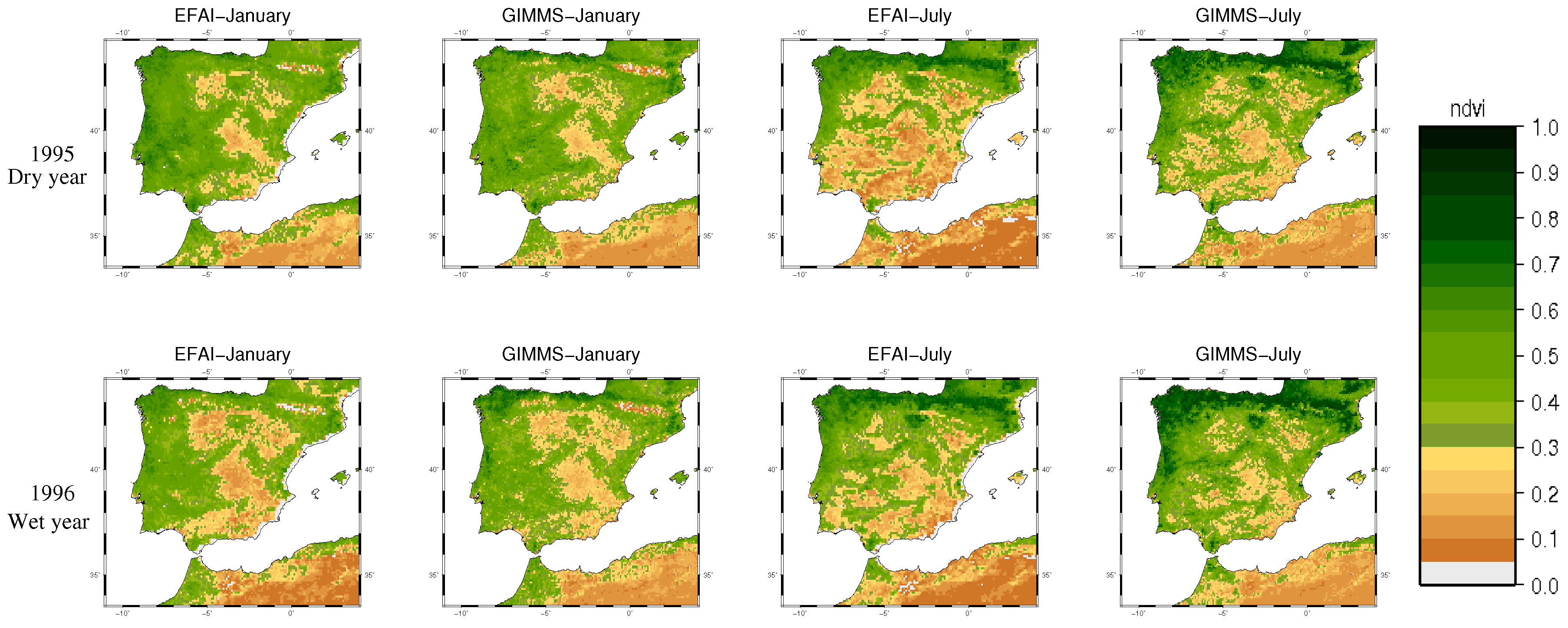
3.1. NDVI Database Comparison

Figure 6 shows the NDVI for the two datasets in a dry year (1995) and a wet year (1996) for January and July over the IP. It is remarkable that they differed in magnitude but that spatial variability was quite similar (spatial correlation over 0.97). The differences were higher when comparing years with different precipitation regime, where NDVI values differed up to 30% in the summer (not shown).
The 12 month run-mean series of the spatially averaged NDVI over the IP for the period 1982–1998 is shown in Figure 7a. The series shows a quite different interannual variability for the whole period; the EFAI-NDVI had a greater variability and lower mean values than the GIMMS-NDVI. We attributed the disagreement (almost a periodical signal not attributable to natural variability) to the solar zenith angle correction implemented in the GIMSS-NDVI that avoids artificial trends derived from orbital drifting. At this point we concluded that the EFAI-NDVI should not be used for characterizing the vegetation properties in RCMs. Therefore, we focused our study on the GIMMS-NDVI data. In addition, GIMMS-NDVI had a longer record, because of the compatibility with AVHRR data with MODIS and SPOT vegetation satellite data, that have continued until nowadays.
Usually FVC is implemented using climatological values in NWPMs and RCMs. We compared the spatially averaged NDVI over the IP, with monthly climatological values calculated on a seven year period (1985–1991) with the monthly evolution on a specific dry (1995) and wet year (1996) (Figure 7b). The biggest NDVI differences between the dry and wet year were observed in spring, when the maximum of vegetation productivity occurred, prevailing these NDVI differences in a lesser way the rest of the year. The spatial average NDVI difference between wet and dry years was about 5% reaching values up to 15% in some areas. This elucidates that taking into account the interannual variability could be important when implementing these data in RCMs.

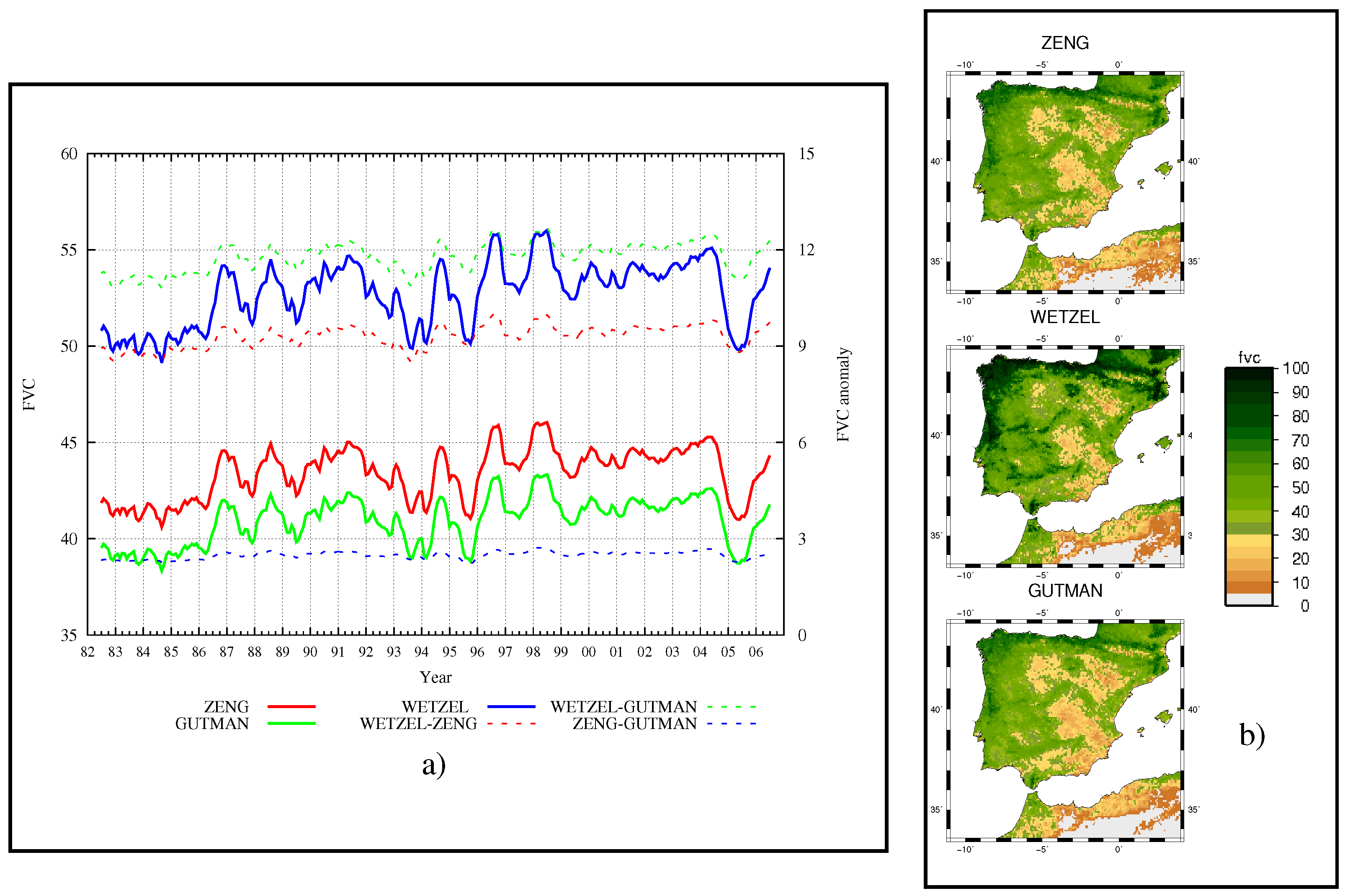
3.2. Analysis of FVC Retrieval Methods

FVC data were obtained for the 25 year of available NDVI data using the three methods. Figure 5a shows the temporal evolution of the FVC data spatially averaged over the IP and Figure 5b the temporal means of FVC values over the domain. Since the three methods used the same NDVI, there was a very good agreement in the temporal variation of FVC, however some important differences appear. The most remarkable difference comparing the magnitude of FVC was that WETZEL method presented FVC values 10% greater than the others. The ZENG and GUTMAN methods only differed around a 3% in magnitude. This large difference was due to the fact that when applying WETZEL method the frequency distribution of NDVI was not taken into account. Regarding the spatial variability, the ZENG and GUTMAN show very similar patterns although the ZENG method achieves a larger range of FVC values, reaching values near 10% and over 80% more frequently.
The differences between the methods depended on the land type by construction. Figure 1b and Figure 2b depict the time series of the FVC spatially averaged by land types calculated with the GUTMAN (green solid line), WETZEL (blue solid line) and ZENG (red solid line) methods as well as the differences between them (dashed lines). The GUTMAN and ZENG methods showed very similar FVC values in forest land types (Figure 1), while the WETZEL method showed significant differences of around 20% respect to the other methods. Land types with low values of FVC, such as shrubland, cropland and grassland (Figure 2) present smaller differences. In the case of closed and open shrubland, the WETZEL method presents the closest values to the other methods. This can be explained because NDVI values below the rupture point of the WETZEL method were more frequent for this land types (Figure 2a).
Therefore, in general, places with high FVC values exhibited a good agreement between the methods that take into account the NDVI frequency distribution (GUTMAN and ZENG), showing larger differences with the WETZEL method. While in places with medium and low values of FVC, the spread among the methods was lower.
Another interesting feature was to evaluate is the differences in phenology. Figure 1 and Figure 2 show the relative frequency distribution if NDVI (a), temporal evolution (b) and FVC annual cycle (c) for each biome and the differences between them. In the biomes where the maximum of FVC occurred in summer, forest vegetation with low hydric stress, the GUTMAN and ZENG methods had a quite similar behavior (maximum value of 60–80% in summer) while the WETZEL method gave greater values. In the rest of the biomes, the maximum of FVC occurred in spring (irrigated lands or places with summer hydric stress) and the differences between the methods were smaller than for forest land types, although there were differences that could be remarkable in cropland, grasslands and woodland areas.

3.3. Sensitivity to the FVC Estimation Method

Here we assessed the sensitivity of climate simulations to the use of different FVC data presented above. For the sake of clarity, we only present the comparisons between the ZENG and WETZEL experiments, because they show the largest FVC differences. Figure 8a depicts the FVC monthly means of ZENG for some months representative of each season (January, April, July and October) and Figure 8b the FVC differences between the ZENG and WETZEL methods. There is a clear negative difference in the FVC estimated (ZENG-WETZEL) with higher FVC values for the WETZEL data, especially in areas with the highest FVC. The biggest difference was in April, when the vegetation productivity presented the maximum rate of generation of biomass.
The effect of such differences between the ZENG and WETZEL data on the regional climate simulations for monthly mean T2m is depicted in Figure 8c,d. In general, lower FVC values led to higher temperatures, but this relationship depended on the time of the year (Figure 8d). This result was directly related to the sensible and latent heat partitioning (not shown). An increase/decrease of vegetation led to a larger/lower evapotranspiration and therefore, a higher/smaller latent heat production. This led to a reduced/intensified sensible heat manifested in a decrease/increase in T2m. Besides, there was an additional effect due to the modification of soil thermal conductivity by the presence of a vegetation canopy. Heat flux from soil was reduced when FVC increases because of heat conductivity was diminished [12,66]. This effect was of importance mostly during night when these fluxes had a dominant role and can cause higher night temperatures with reduced FVC.
It is worth noting that T2m differences were higher in April and July than in January and October with similar FVC differences (Figure 8). In January differences of 30% in FVC led to changes smaller than 0.5 C, while in July or April can reach 1 C in some places. This was mainly due to the greater availability of energy at these months. In addition, the greater dispersion in the quasi-linear relationship between changes in FVC and T2m (Figure 8d) for higher Δ F V C values may be relevant. Therefore, it was clear that changing the FVC database modified the climatology reproduced by a RCM, both the spatial patterns and the amplitude of the annual cycle.

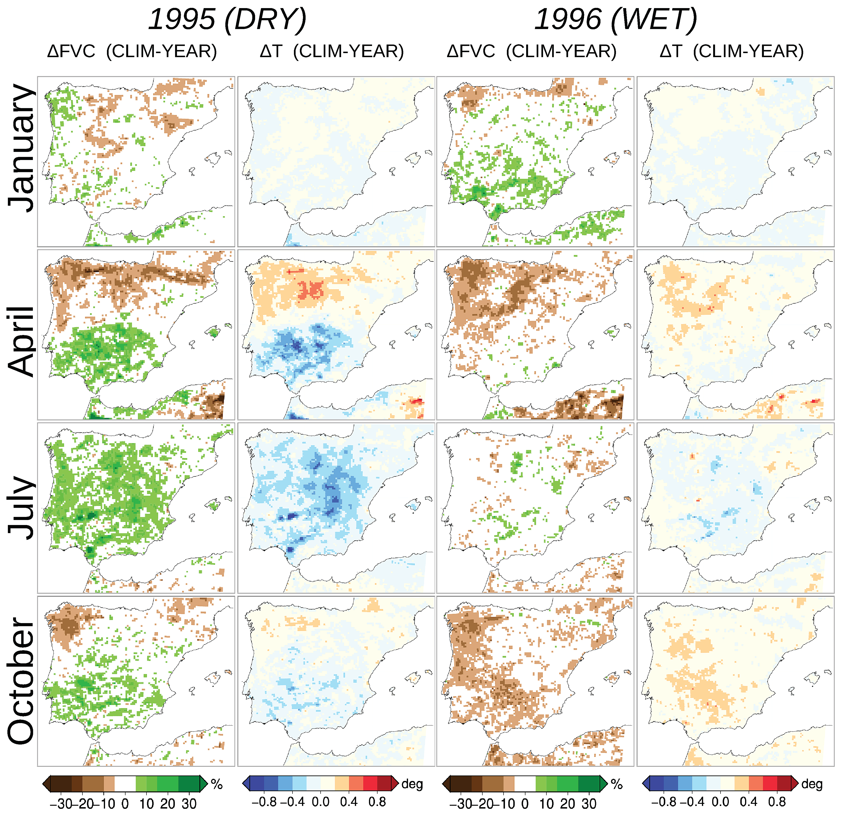
3.4. Sensitivity to FVC Interannual Variations

As mentioned above, in RCM experiments, FVC values are usually prescribed using climatologies, so they do not vary from year to year. But vegetation depended on the climate conditions as well as other factors, and it had a non negligible interannual variability. In this section we analyze the effect of varying the FVC according to the observations (real FVC) versus fixed monthly climatological/prescribed values.
Figure 9 shows the differences between the FVC 5-year climatology simulation (CLIM) and the reconstructed (YEAR) for January, April, July and October for two years, the dry 1995 and wet 1996. These years were selected because of their quite different climate conditions. Dry conditions prevailed during 1995, while 1996 was characterized for abundant precipitation that favored higher biomass production.
During the dry year, the prescribed FVC was much higher that the estimated for this year, finding large areas with Δ F V C over 10%, especially in April and July that locally reached values around 30%. The T2m temperature patterns resembled the spatial structure of Δ F V C with a clear negative bias. The largest T2m differences appeared again in July and April, with values larger than 0.4 C in large areas that locally were over 0.8 C.
During the wet year the largest Δ F V C appeared in April in the north–west part of the IP, and October over the South and Western Iberia. In this case differences were negative, i.e., the prescribed FVC underestimates the YEAR FVC. Interestingly, the absolute T2m differences were smaller, with slightly lower absolute Δ F V C . This is due to the fact that in July (highest sensitivity) Δ F V C is quite small, and that in April advection phenomena prevailed in the area with the largest Δ F V C .
Adding both effects at the different times suggest that interannual variability can change more that 1 C in some areas for a given month.

4. Discussion and Conclusions

Three database of monthly FVC from 1982 to 2006 has been created for a domain covering the whole IP with a spatial resolution of 0.1 with the aim of being implemented in RCMs to improve climate simulations by providing more realistic soil physical conditions. Three different methodologies, WETZEL, GUTMAN and ZENG, were applied to the same NDVI database. The GIMMS-NDVI data was selected because it has better interannual behavior, longer record and is compatible with MODIS and SPOT vegetation data, which facilitates its temporal extension.
The comparison between the FVC databases reveals important differences between them that depend on the FVC value and the biome, being especially relevant for forest land types. Methods that use the frequency distribution of NVDI (ZENG and GUTMAN) are more similar although some differences can be found between them depending of the land type. In addition the FVC series reveal a important interannual variability, consequently prescribed FVC values can present important differences regarding the “real” FVC. These facts can be important when FVC are used in RCMs coupled to LSMs. The magnitude of the differences found causes a noteworthy impact on surface fluxes and hence modifying the regional climate.
The RCM experiments performed exhibit a not negligible effect of FVC uncertainty on the monthly climatological values. The results showed that differences of 30% of FVC, that appear in the two sensitivity experiments, can produce bias of 1 in T2m monthly values. Therefore, depending on the spatial structure of the FVC differences, the climatological patters are modified. In addition, the magnitude of the model response depends on the time of the year. This implies that the annual cycle reproduced by the model is also sensible to the FVC data used. Finally, the role of the interannual variability of the FVC series can also change the interannual variability of climatological series (T2m in our study). In the experiment showed here, the differences for some times of the year, especially spring and summer could reach 1 C.
It is known that changes in vegetation also modifies the albedo. This was not taken into account in our experiments. Therefore, it can be expected an impact on the regional climate simulations. In fact, this impacts can be opposite to our findings since a decrease of the vegetation leads to an increase of albedo and then, less radiation is trapped by the surface and temperature could decrease. However, Crawford et al. [31] show that the impact of changing albedo on surface heat fluxes is much smaller, an order of magnitude, than changing FVC.
In this paper we just analyze the sensitivity of RCM simulations to changes in FVC. A question remaining is if the RCM simulations with these new FVC datasets can better capture the climate over the IP. The sensitivity of the model to the FVC changes is much smaller than the deviations of the model respect to the observations (not shown), therefore it is difficult to find any improvement using only one or two years of data. This is not a surprising result. For example, Gómez-Navarro et al. [67] shows that the skill score of different RCMs depends on the data-base chosen for evaluating the model. Other examples can be found in Fernández et al. [68] and Jerez et al. [64] where the authors did not find any combination of physical parameterizations that always reproduce better the observed climate. However, changing FVC with time instead of using climatological data should improve the simulation of inter-annual regional climate variability. For instance, the mean temperature differences between the dry and the wet year are better represented by the YEAR simulations (not shown).
In this work, just linear models have been tested for obtaining FVC from NDVI, because they have been more frequently used (for instance, in most of works cited along the work). Some examples are the NOAH land–surface model and the NAM Eta model. However, some authors use quadratics models. Figure 3 shows the relationship between FVC and NDVI for the linear models analyzed and a quadratic model (GUTMAN Quadratic). The quadratic methodology drives to lower values of FVC. Anyway, the FVC differences obtained with linear methods covers the range of the differences in FVC that we found.

Author Contributions

Conceptualization, J.M.J.-G. and J.P.M. Methodology, J.M.J.-G. and J.P.M. Software, J.M.J.-G. and J.P.M. and S.J. Investigation, J.M.J.-G. Formal Analysis, J.M.J.-G., J.P.M. and S.J. Data curation, J.M.J.-G., J.P.M. and S.J. Writing—original draft preparation, J.M.J.-G. and J.P.M. Writing—review and editing, J.M.J.-G., J.P.M., S.J. and F.V. Visualization, J.M.J.-G. Supervision, J.P.M. and F.V.

Funding

The authors acknowledge projects REPAIR-CGL2014-59677-R and ACEX-CGL2017-87921-R of the Spanish Ministry of Economy and Competitiveness PCIN-2014-013-C07-04, PCIN2016-080 (UE ERA-NET Plus NEWA Project), CGL2016-78702, and the Instituto de Matemática Interdisciplinar (IMI) of the Universidad Complutense that partially support this work. S. Jerez has received funding from the Plan Propio de Investigación of the University of Murcia (grant No. UMU-2017-10604) and the Fundación Séneca—Regional Agency for Science and Technology of Murcia (CLIMAX project 20642/JLI/18).

Acknowledgments

We acknowledge all the institutions and communities that provided free software, R community, CDO (Climate Data Operators), GMT (Generic Mapping Tools), MM5, Gnuplot, gfortran as well as the institutions supplying data (ECMWF, NASA).

Conflicts of Interest

The authors declare no conflicts of interest.

References

  1. Pielke, R.A. Overlooked issues in the U.S. National Climate and IPCC assesments. Clim. Chang. 2002, 52, 1–11. [Google Scholar]
  2. Godfrey, C.M.; Stensrud, D.J.; Leslie, L.M. The influence of improved land surface and soil data on mesoscale model predictions. CD–ROM. In Proceedings of the 19th Conference on Hydrology; American Meteorological Society: Boston, MA, USA, 2002; Paper 4.7. [Google Scholar]
  3. Jerez, S.; Montavez, J.; Gomez-Navarro, J.; Jimenez, P.; Jimenez-Guerrero, P.; Lorente, R.; Gonzalez-Rouco, J.F. The role of the land-surface model for climate change projections over the Iberian Peninsula. J. Geophys. Res. Atmos. 2012, 117. [Google Scholar] [CrossRef] [Green Version]
  4. Stensrud, D.J. Parameterization Schemes: Keys to Understanding Numerical Weather Prediction Models; Cambridge University Press: Cambridge, UK, 2007. [Google Scholar]
  5. Chang, J.T.; Wetzel, P.J. Effects of spatial variations of soil moisture and vegetation on the evolution of a prestorm environment: A numerical case study. Mon. Weather Rev. 1991, 119, 1368–1390. [Google Scholar] [CrossRef]
  6. Gutman, G.; Ignatov, A. The derivation of the green vegetation fraction from NOAA/AVHRR data for use in numerical weather prediction models. Int. J. Remote Sens. 1998, 19, 1533–1543. [Google Scholar] [CrossRef]
  7. Zeng, X.; Dickinson, R.E.; Walker, A.; Shaikh, M. Derivation and evaluation of global 1-km fractional vegetation cover data for land modelling. J. Appl. Meteorol. 2000, 39, 826–839. [Google Scholar] [CrossRef]
  8. Li, X.; Zhang, J. Derivation of the Green Vegetation Fraction of the Whole China from 2000 to 2010 from MODIS Data. Earth Interact. 2016, 20, 1–16. [Google Scholar] [CrossRef]
  9. Carlson, T.N.; Perry, E.M.; Schmugge, T.J. Remote estimates of soil moisture availability and fractional vegetation cover for agricultural fields. Remote Sens. Environ. 1990, 52, 45–70. [Google Scholar]
  10. Sellers, P.J.; Los, S.O.; Tucker, C.J.; Justice, C.O.; Dazlich, D.A.; Collatz, G.J.; Randall, D.A. A revised land surface parameterization (SiB2) for atmospheric GCMs. Part II: The generation of global fields of terrestrial biophysical parameters from satellite data. J. Clim. 1996, 9, 706–737. [Google Scholar] [CrossRef]
  11. Hanamean, J.M., Jr.; Pielke, R.A., Sr.; Castro, C.L.; Ojima, D.S.; Reed, B.C.; Gao, Z. Vegetation greenness impacts on maximum and minimum temperatures in northeast Colorado. Meteorol. Appl. 2003, 10, 203–215. [Google Scholar] [CrossRef] [Green Version]
  12. Ek, M.B.; Mitchell, K.E.; Lin, Y.; Rogers, E.; Grunmann, P.; Koren, V.; Gayno, G.; Tarpley, J.D. Implementation of Noah land surface model advances in the National Centers for Environmental Prediction operational mesoscale Eta model. J. Geophys. Res. Atmos. 2003, 108, 8851. [Google Scholar] [CrossRef]
  13. Kurkowski, N.P.; Stensrud, D.J.; Baldwin, M.E. Assessment of Implementing Satellite-Derived Land Cover Data in the Eta Model. Weather Forecast. 2003, 18, 404–416. [Google Scholar] [CrossRef]
  14. Marshall, C.H.; Crawford, K.C.; Mitchell, K.E.; Stensrud, D.J. The impact of the land surface physics in the operational NCEP Eta model on simulating the diurnal cycle: Evaluation and testing using Oklahoma Mesonet data. Weather Forecast. 2003, 18, 748–768. [Google Scholar] [CrossRef]
  15. Hong, S.; Lakshmi, V.; Small, E.; Chen, F.; Tewari, M.; Manning, K.W. Effects of vegetation and soil moisture on the simulated land surface processes from the coupled WRF/Noah model. J. Geophys. Res. Atmos. 2009, 114, D18118. [Google Scholar] [CrossRef]
  16. Limei, R.; Gilliam, R.; Binkowski, F.; Xiu, A.; Pleim, J.; Band, L. Sensitivity of the Weather Research and Forecast/Community Multiscale Air Quality modeling system to MODIS LAI, FPAR, and albedo. J. Geophys. Res. Atmos. 2015, 120, 8491–8511. [Google Scholar] [Green Version]
  17. Cao, Q.; Yu, D.; Georgescu, M.; Han, Z.; Wu, J. Impacts of land use and land cover change on regional climate: A case study in the agro-pastoral transitional zone of China. Environ. Res. Lett. 2015, 10, 124025. [Google Scholar] [CrossRef]
  18. Xu, L.; Pyles, R.D.; Snyder, R.H.; Monier, E.; Falk, M.; Chen, S.-H. Impact of canopy representations on regional modeling of evapotranspiration using the WRF-ACASA coupled model. Agric. For. Meteorol. 2017, 247, 79–92. [Google Scholar] [CrossRef] [Green Version]
  19. Zhang, M.; Geping, L.; Maeyer, P.D.; Cai, P.; Kurban, A. Improved Atmospheric Modelling of the Oasis-Desert System in Central Asia Using WRF with Actual Satellite Products. Remote Sens. 2017, 9, 1273. [Google Scholar] [CrossRef]
  20. Wen, J.; Lai, X.; Shi, X.; Pan, X. Numerical simulations of fractional vegetation coverage influences on the convective environment over the source region of the Yellow River. Meteorol. Atmos. Phys. 2013, 120, 1–10. [Google Scholar] [CrossRef]
  21. Meng, X.H.; Evans, J.P.; McCabe, M.F. The Impact of Observed Vegetation Changes on Land–Atmosphere Feedbacks During Drought. J. Hydrometeorol. 2014, 15, 759–776. [Google Scholar] [CrossRef] [Green Version]
  22. Müller, O.V.; Berbery, E.H.; Alcaraz-Segura, D.; Ek, M.B. Regional model simulations of the 2008 drought in southern South America using a consistent set of land surface properties. J. Clim. 2014, 27, 6754–6778. [Google Scholar] [CrossRef]
  23. Matsui, T.; Lakshmi, V.; Small, E.E. The effects of satellite-derived vegetation cover variability on simulated land-atmosphere interactions in the NAMS. J. Clim. 2005, 18, 21–40. [Google Scholar] [CrossRef]
  24. Notaro, M.; Chen, G.; Yu, Y.; Wang, F.; Tawfik, A. Regional Climate Modeling of Vegetation Feedbacks on the Asian–Australian Monsoon Systems. J. Clim. 2017, 30, 1553–1582. [Google Scholar] [CrossRef]
  25. James, K.A.; Stensrud, D.J.; Yussouf, N. Value of real-time vegetation fraction to forecasts of severe convection in high-resolution models. Weather Forecast. 2009, 24, 187–210. [Google Scholar] [CrossRef]
  26. Zhang, G.; Zhou, G.; Chen, F.; Barlage, M.; Xue, L. A Trial to Improve Surface Heat Exchange Simulation through Sensitivity Experiments over a Desert Steppe Site. J. Hydrometeorol. 2014, 15, 664–684. [Google Scholar] [CrossRef]
  27. Vahmani, P.; Hogue, T. High-resolution land surface modeling utilizing remote sensing parameters and the Noah UCM: A case study in the Los Angeles Basin. Hydrol. Earth Syst. Sci. 2014, 18, 4791–4806. [Google Scholar] [CrossRef]
  28. Vahmani, P.; Ban-Weiss, G. Climatic consequences of adopting drought-tolerant vegetation over Los Angeles as a response to California drought. Geophys. Res. Lett. 2016, 43, 8240–8249. [Google Scholar] [CrossRef]
  29. Stockli, R.; Vidale, P.L. European plant phenology and climate as seen in a 20 year AVHRR land-surface parameter dataset. Int. J. Remote Sens. 2004, 17, 3303–3330. [Google Scholar] [CrossRef]
  30. Miller, J.; Barlage, M.; Zeng, X.; Wei, H.; Mitchell, K. Sensitivity of the NCEP/Noah land surface model to the MODIS green vegetation fraction data set. Geophys. Res. Lett. 2006, 33, 237–250. [Google Scholar] [CrossRef]
  31. Crawford, T.M.; Stensrud, D.J.; Mora, F.; Merchant, J.W.; Wetzel, P.J. Value of Incorporating Satellite-Derived Land Cover Data in MM5/PLACE for Simulating Surface Temperatures. J. Hydrometeorol. 2001, 2, 453–468. [Google Scholar] [CrossRef]
  32. Myneni, R.B.; Keeling, C.D.; Tucker, C.J.; Asrar, G.; Nemani, R.R. Increased plant growth in the northern high latitudes from 1981 to 1991. Nature 1997, 386, 698–702. [Google Scholar] [CrossRef]
  33. Refslund, J.; Dellwik, E.; Hahmann, A.; Barlage, M.; Boegh, E. Development of satellite green vegetation fraction time series for use in mesoscale modeling: Application to the European heat wave 2006. Theor. Appl. Clim. 2014, 117, 377–392. [Google Scholar] [CrossRef]
  34. Pettorelli, N.; Olav, V.J.; Atle, M.; Gaillard, J.M.; Tucker, C.J.; Stenseth, N.C. Using the satellite-derived NDVI to assess ecological responses to enviromental change. IEEE Trans. Geosci. Remote Sens. 2005, 20, 503–510. [Google Scholar]
  35. Myneni, R.B.; Hall, F.G.; Sellers, P.J.; Marshak, A.L. The interpretation of spectral vegetation indexes. IEEE Trans. Geosci. Remote Sens. 1995, 33, 481–486. [Google Scholar] [CrossRef]
  36. Zhou, L.; Kaufmann, R.K.; Tian, Y.; Mineny, R.B.; Tucker, C.J. Relation between interannual variations in satellite measures of northern forest greenness and climate between 1982 and 1999. J. Geophys. Res. 2003, 108. ACL 3-1–ACL 3-16. [Google Scholar] [CrossRef]
  37. Tucker, C.J.; Pinzon, J.E.; Brown, M.E.; Slayback, D.; Pak, E.W.; Mahoney, R.; Vermote, E.; Saleous, N.E. An Extended AVHRR 8-km NDVI Data Set Compatible with MODIS and SPOT Vegetation NDVI Data. Int. J. Remote Sens. 2005, 26, 4485–4498. [Google Scholar]
  38. Tarpley, J.P.; Schneider, S.R.; Money, R.L. Global vegetation indices from NOAA-7 meteorological satellite. J. Clim. Appl. Meteorol. 1984, 23, 491–494. [Google Scholar]
  39. Gutman, G.; Tarpley, D.; Ignatov, A.; Olson, S. The enhanced NOAA Global Land datasets from the Advanced Very High Resolution Radiometer. Int. J. Remote Sens. 1995, 76, 1141–1156. [Google Scholar] [CrossRef]
  40. James, M.E.; Kalluri, S.N.V. The Pathfinder AVHRR land dataset:an improved coarse resolution dataset for terrestrial monitoring. Int. J. Remote Sens. 1994, 15, 3347–3363. [Google Scholar] [CrossRef]
  41. Pinzon, J. Using HHT to successfully uncouple seasonal and interannual components in remotely sensed data. In Proceedings of the 6th World Multiconference on Systemics, Cybernetics and Informatics, Orlando, FL, USA, 14–18 July 2002. [Google Scholar]
  42. Tucker, C.J.; Pinzon, J.E.; Brown, M.E. Global Inventory Modeling and Mapping Studies 2.0, 2004. Digital Media. Available online: http://staff.glcf.umd.edu/sns/htdocs/data/gimms/ (accessed on 8 March 2019).
  43. Gallo, K.; Tarpley, D.; Mitchell, K.; Csiszar, I.; Owen, T.; Reed, B. Monthly fractional green vegetation cover associated with land cover classes of the Conterminous USA. Geophys. Res. Lett. 2001, 28, 2089–2092. [Google Scholar] [CrossRef]
  44. Montandon, L.M.; Small, E.E. The impact of soil reflectance on the quantification of the green vegetation fraction from NDVI. Remote Sens. Environ. 2008, 112, 1835–1845. [Google Scholar] [CrossRef]
  45. Carlson, T.N.; Rypley, D.A. On the relation between NDVI, fractional vegetation cover, and leaf area index. Remote Sens. Environ. 1997, 62, 241–252. [Google Scholar] [CrossRef]
  46. Price, J.C. Estimating vegetation amount from visible and near infrared reflectances. Remote Sens. Environ. 1992, 41, 29–34. [Google Scholar] [CrossRef]
  47. Hansen, M.; DeFries, R.; Townshend, J.R.G.; Sohlberg, R. UMD Global Land Cover Classification. 8 Kilometer. Version 1.0. 1981–1994; Department of Geography, University of Maryland: College Park, MD, USA, 1998. [Google Scholar]
  48. Hansen, M.; DeFries, R.; Townshend, J.R.G.; Sohlberg, R. Global land cover classification at 1km resolution using a decision tree classifier. Int. J. Remote Sens. 2000, 21, 1331–1365. [Google Scholar] [CrossRef]
  49. Grell, G.; Dudhia, J.; Stauffer, D. A Description of the Fifth-Generation Penn State/NCAR Mesoscale Model (MM5); NCAR Technik Note; NCAR: Boulder, CO, USA, 1994. [Google Scholar]
  50. Jerez, S.; Montavez, J.P.; Gomez-Navarro, J.J.; Jimenez-Guerrrero, P.; Jimenez, J.M.; Gonzalez-Rouco, J.F. Temperature sensitivity to the land-surface model in MM5 climate simulations over the Iberian Peninsula. Meteorol. Z. 2010, 19, 363–374. [Google Scholar] [CrossRef] [Green Version]
  51. Dee, D.P.; Uppala, S.M.; Simmons, A.; Berrisford, P.; Poli, P.; Kobayashi, S.; Andrae, U.; Balmaseda, M.A.; Balsamo, G.; Bauer, P.; et al. The ERA-Interim reanalysis: Configuration and performance of the data assimilation system. Quart. J. R. Meteorol. Soc. 2011, 137, 553–597. [Google Scholar] [CrossRef]
  52. Grell, G.A. Prognostic evaluation of assumptions used by cumulus parameterizations. Mon. Weather Rev. 1993, 121, 764–787. [Google Scholar] [CrossRef]
  53. Dudhia, J. Numerical study of convection observed during the winter monsoon experiment using a mesoscale two-dimensional model. J. Atmos. Sci. 1989, 46, 3077–3107. [Google Scholar] [CrossRef]
  54. Mlawer, E.; Taubman, S.; Brown, P.; Iacono, M.; Clough, S. Radiative transfer for inhomogeneous atmospheres: RRTM, a validated correlated-k model for the longwave. J. Geophys. Res. 1997, 102, 16663–16682. [Google Scholar] [CrossRef] [Green Version]
  55. Hong, S.; Pan, H. Nonlocal boundary layer vertical diffusion in a Medium-Range Forecast Model. Mon. Weather Rev. 1996, 124, 2322–2339. [Google Scholar] [CrossRef]
  56. Chen, F.; Dudhia, J. Coupling an advanced land-surface/hydrology model with the Penn State/NCAR MM5 modeling system. Part I: Model implementation and sensitivity. Mon. Weather Rev. 2001, 129, 569–585. [Google Scholar] [CrossRef]
  57. Mahrt, L.; Ek, M. The influence of atmospheric stability on potential evaporation. J. Appl. Meteorol. 1984, 23, 222–234. [Google Scholar] [CrossRef]
  58. Mahrt, L.; Pan, H. A two-layer model of soil hydrology. Bound. Layer Meteorol. 1984, 29, 1–20. [Google Scholar] [CrossRef] [Green Version]
  59. Pan, H.L.; Mahrt, L. Interaction between soil hydrology and boundary-layer development. Bound. Layer Meteorol. 1987, 38, 185–202. [Google Scholar] [CrossRef]
  60. Chen, F.; Mitchell, K.; Schaake, J.; Xue, Y.; Pan, H.L.; Koren, V.; Duan, Q.Y.; Ek, M.; Betts, A. Modeling of land surface evaporation by four schemes and comparison with FIFE observations. J. Geophys. Res. Atmos. 1996, 101, 7251–7268. [Google Scholar] [CrossRef] [Green Version]
  61. Noilhan, J.; Planton, S. A simple parameterization of land surface processes for meteorological models. Mon. Weather Rev. 1989, 117, 536–549. [Google Scholar] [CrossRef]
  62. Jacquemin, B.; Noilhan, J. Sensitivity study and validation of a land surface parameterization using the HAPEX-MOBILHY data set. Bound. Layer. Meteorol. 1990, 52, 93–134. [Google Scholar] [CrossRef]
  63. Gómez-Navarro, J.; Montávez, J.; Jiménez-Guerrero, P.; Jerez, S.; Lorente-Plazas, R.; González-Rouco, J.; Zorita, E. Internal and external variability in regional simulations of the Iberian Peninsula climate over the last millennium. Clim. Past 2012, 8, 25. [Google Scholar] [CrossRef]
  64. Jerez, S.; Montavez, J.P.; Jimenez-Guerrero, P.; Gomez-Navarro, J.J.; Lorente-Plazas, R.; Zorita, E. A multi-physics ensemble of present-day climate regional simulations over the Iberian Peninsula. Clim. Dyn. 2013, 40, 3023–3046. [Google Scholar] [CrossRef]
  65. Lorente-Plazas, R.; Montávez, J.; Jerez, S.; Gómez-Navarro, J.; Jiménez-Guerrero, P.; Jiménez, P. A 49 year hindcast of surface winds over the Iberian Peninsula. Int. J. Climatol. 2015, 35, 3007–3023. [Google Scholar] [CrossRef]
  66. Peters-Lidard, C.D.; Zion, M.S.; Wood, E.F. A soil-vegetation-atmosphere transfer scheme for modeling spatially variable water and energy balance processes. J. Geophys. Res. Atmos. 1997, 102, 4303–4324. [Google Scholar] [CrossRef] [Green Version]
  67. Gómez-Navarro, J.; Montávez, J.; Jerez, S.; Jiménez-Guerrero, P.; Zorita, E. What is the role of the observational dataset in the evaluation and scoring of climate models? Geophys. Res. Lett. 2012, 39. [Google Scholar] [CrossRef] [Green Version]
  68. Fernández, J.; Montávez, J.; Sáenz, J.; González-Rouco, J.; Zorita, E. Sensitivity of the MM5 mesoscale model to physical parameterizations for regional climate studies: Annual cycle. J. Geophys. Res. Atmos. 2007, 112. [Google Scholar] [CrossRef] [Green Version]
Figure 1. (a) Area covered by land type. Relative frequency distributions of NDVI in the IP by land types according to UMD global landcover. (b) FVC time series in forest land types calculated with the GUTMAN (green solid line), WETZEL (blue solid line) and ZENG (red solid line) methods (spatial average by land type). Differences between FVC methods: WETZEL-ZENG (red dashed line), WETZEL-GUTMAN (green dashed line), ZENG-GUTMAN (blue dashed line). (c) Same as b but monthly averaged values by land type for the period 1982–2006.
Atmosphere 10 00281 g001
Figure 2. As Figure 1 for closed and open shrubland, grassland and croplands.
Atmosphere 10 00281 g002
Figure 3. Relationship between fractional vegetation cover (FVC) and nearest difference vegetation index (NDVI) for the ZENG (red area), GUTMAN, WETZEL, and GUTMAN quadratic methods.
Atmosphere 10 00281 g003
Figure 4. Regional climate model (RCM) spatial domains. Mother domain, D1 (30 km), and inner domain, D2 (10 km). Topography of the spatial domains.
Atmosphere 10 00281 g004
Figure 5. (a) FVC spatial averaged time series (solid lines) and differences between them (dashed lines) for the whole IP calculated by the WETZEL (blue line), GUTMAN (green line) and ZENG (red line) methods. (b) FVC temporal averaged over the whole period (1982–2006) for the IP for the ZENG, WETZEL and GUTMAN methods.
Atmosphere 10 00281 g005
Figure 6. EFAI-NDVI and GIMMS-NDVI for January and July for a wet year (1996) and a dry year (1995) in the Iberian Peninsula (IP).
Atmosphere 10 00281 g006
Figure 7. (a) NDVI 12 month run-mean of the spatially averaged series for the IP derived from the EFAI-NDVI (red line) and GIMMS-NDVI (green line); (b) GIMMS-NDVI monthly values for a wet year (1996, green line), a dry year (1995, orange line) and climatology (blue line).
Atmosphere 10 00281 g007
Figure 8. (a) Monthly means of FVC for the ZENG method. (b) Differences of monthly means of FVC between the ZENG and WETZEL methods. (c) Differences in monthly means of T2m between the ZENG and WETZEL regional climate simulations. (d) x–y scatter plot graph between differences of FVC (x-axis) and differences in T2m between ZENG and WETZEL methods(y-axis).
Atmosphere 10 00281 g008
Figure 9. Differences between five-year FVC climatology (CLIM) simulation (climatology-based FVC) and FVC values for such year (YEAR) simulation (inter-annual varying FVC) for FVC and T2m in a dry year (1995) and a wet year (1996).
Atmosphere 10 00281 g009

