Assessing Forest Canopy Impacts on Smoke Concentrations Using a Coupled Numerical Model

 , , , , , ,
  ,
, 
Abstract
1. Introduction
2. Methods
2.1. Prescribed Fire Cases and Field Measurements
2.2. ARPS-CANOPY Numerical Weather Prediction Model
2.3. FLEXPART-WRF Lagrangian Particle Dispersion Model
3. Results and Discussion
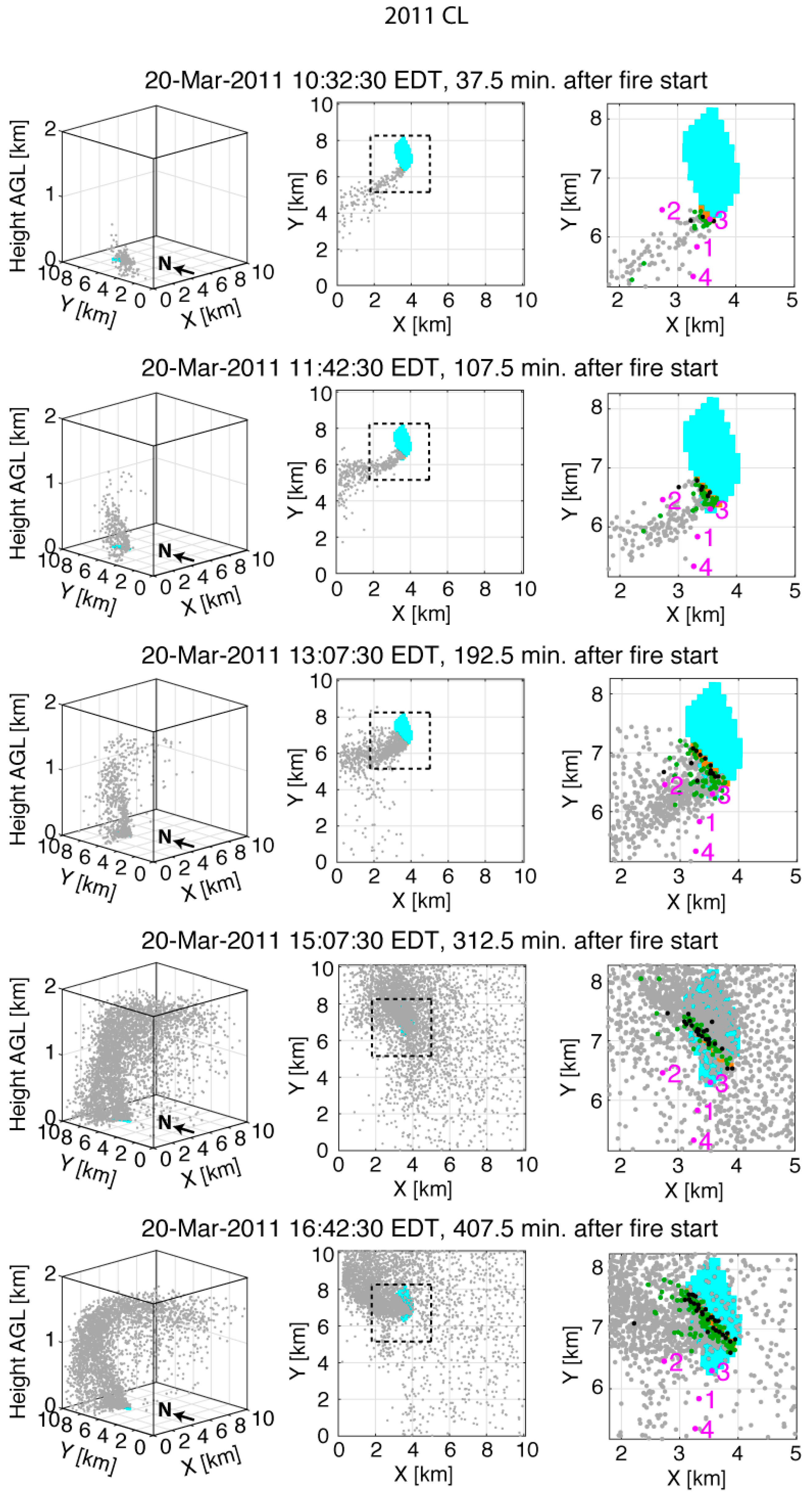
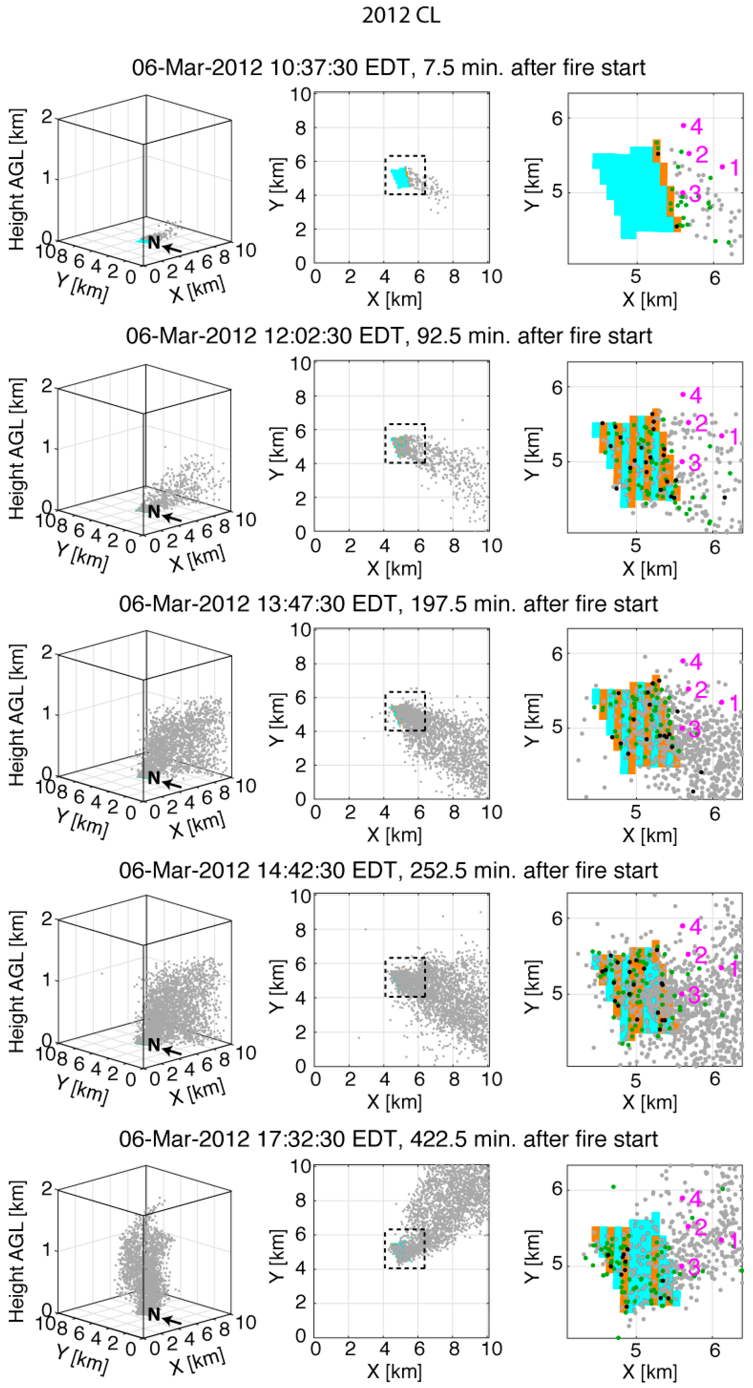
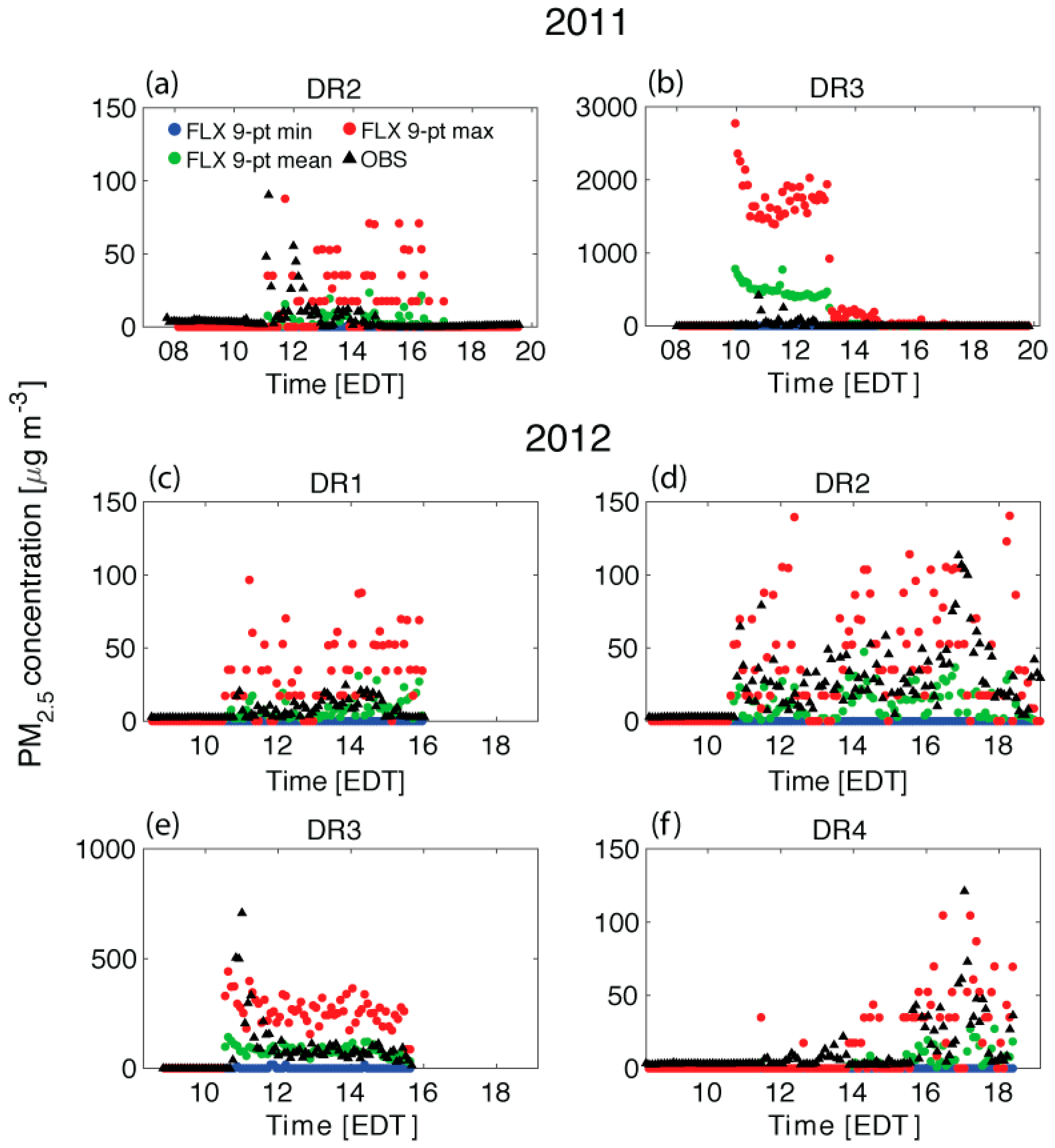
3.1. Smoke Plume Overview and AC/F Assessment
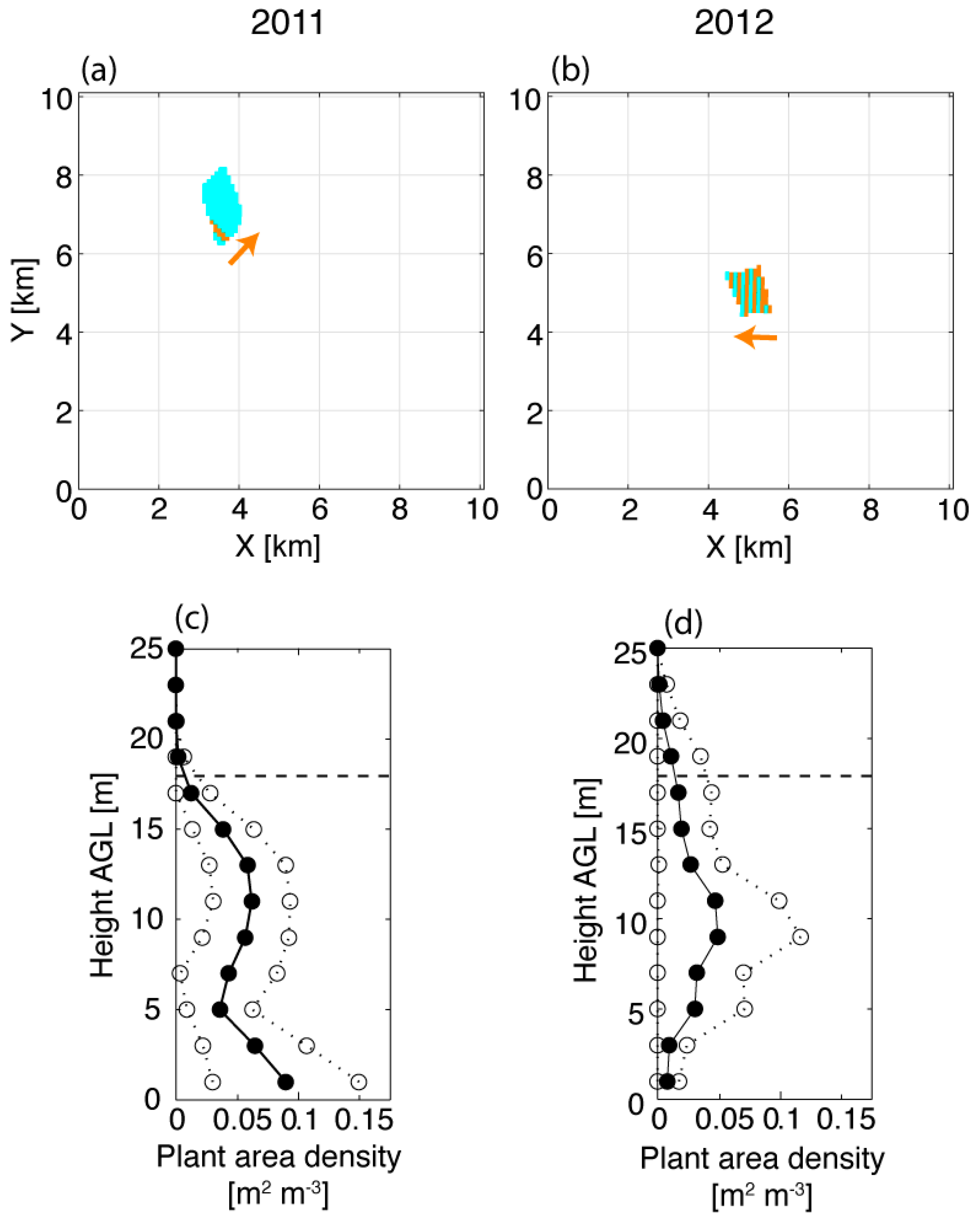
3.2. Smoke Plume Sensitivity to the Forest Canopy
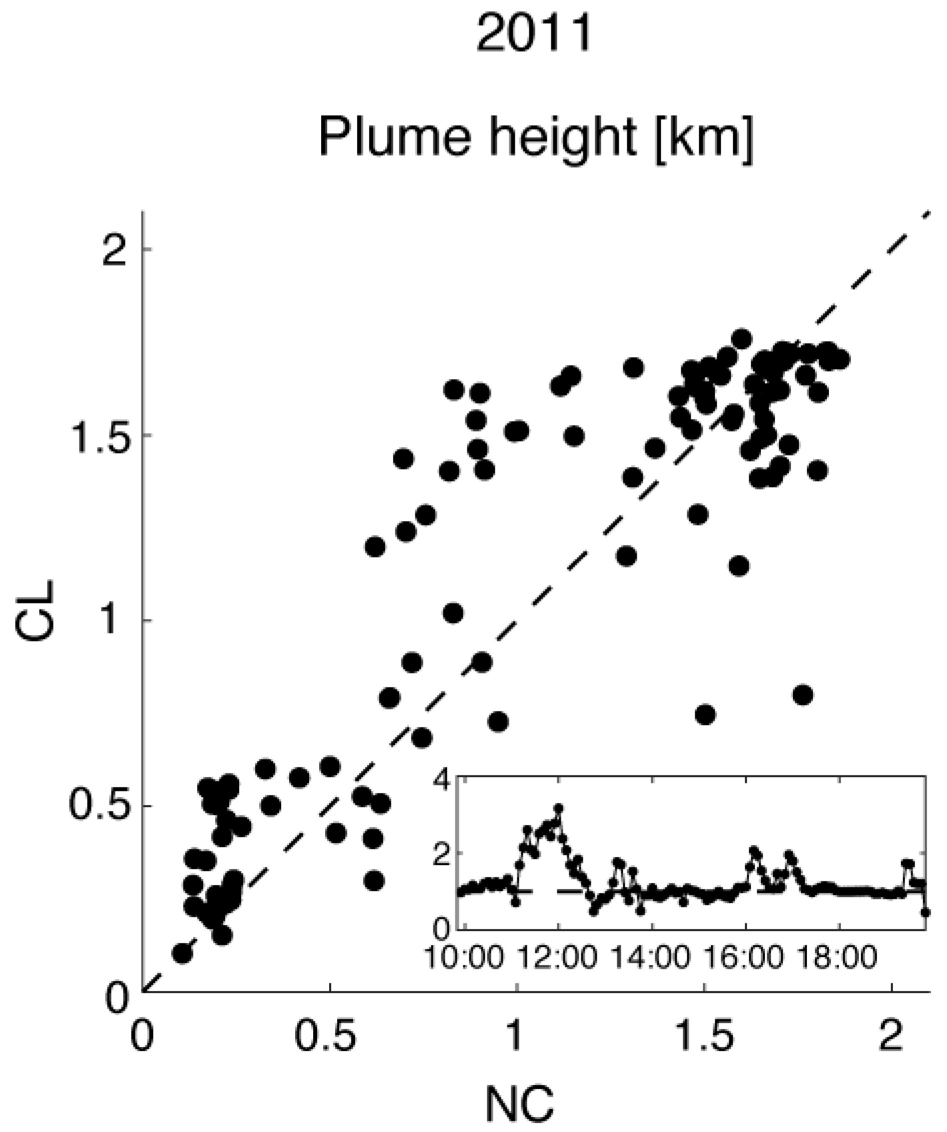
3.2.1. 2011 Case
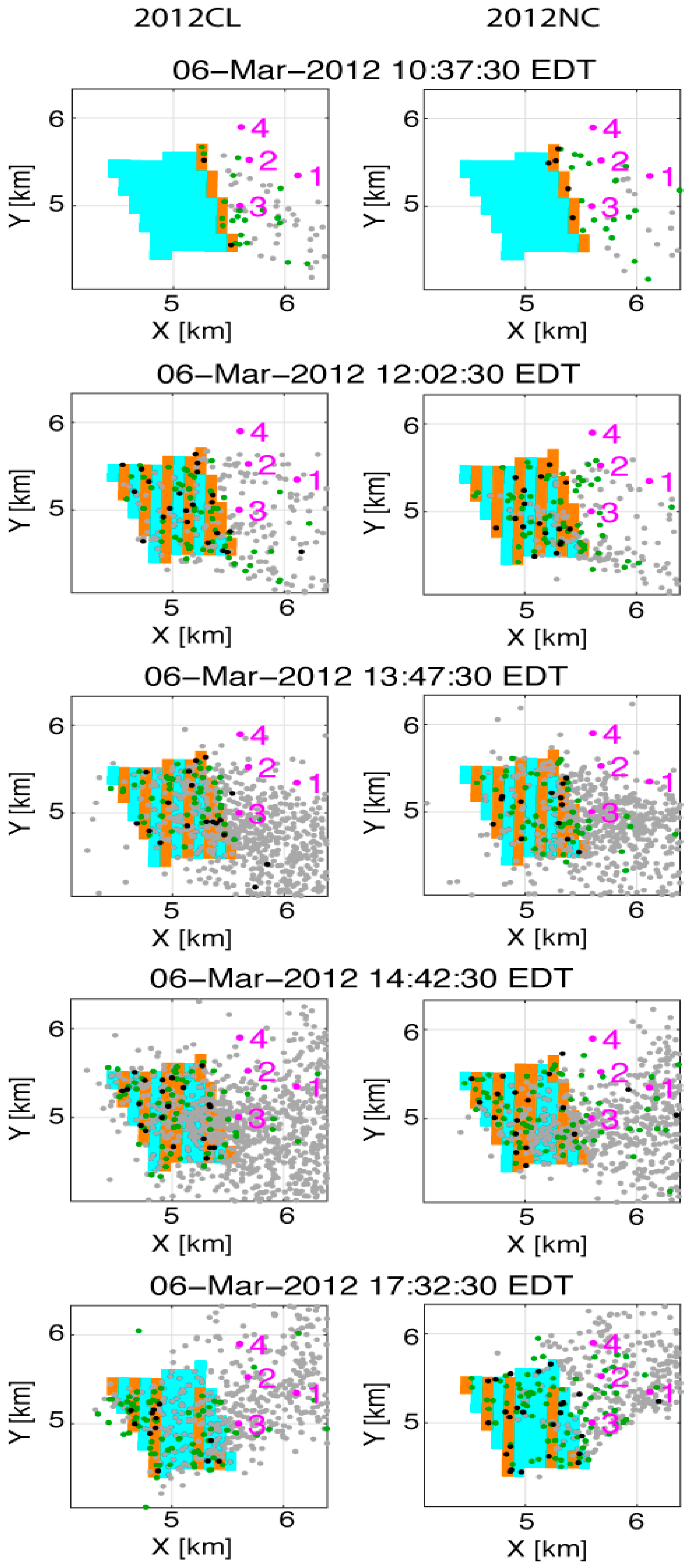
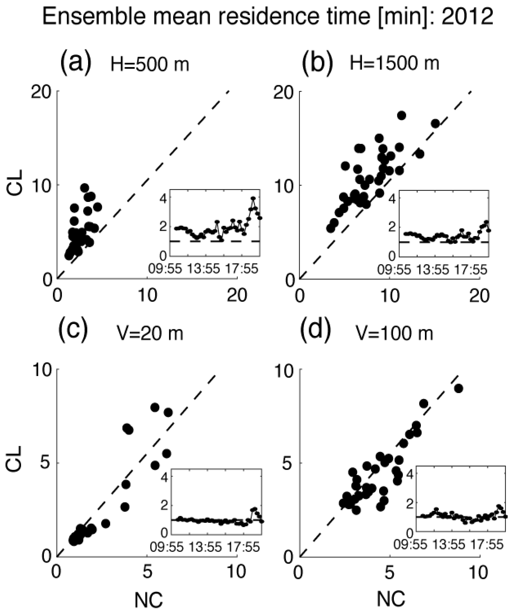
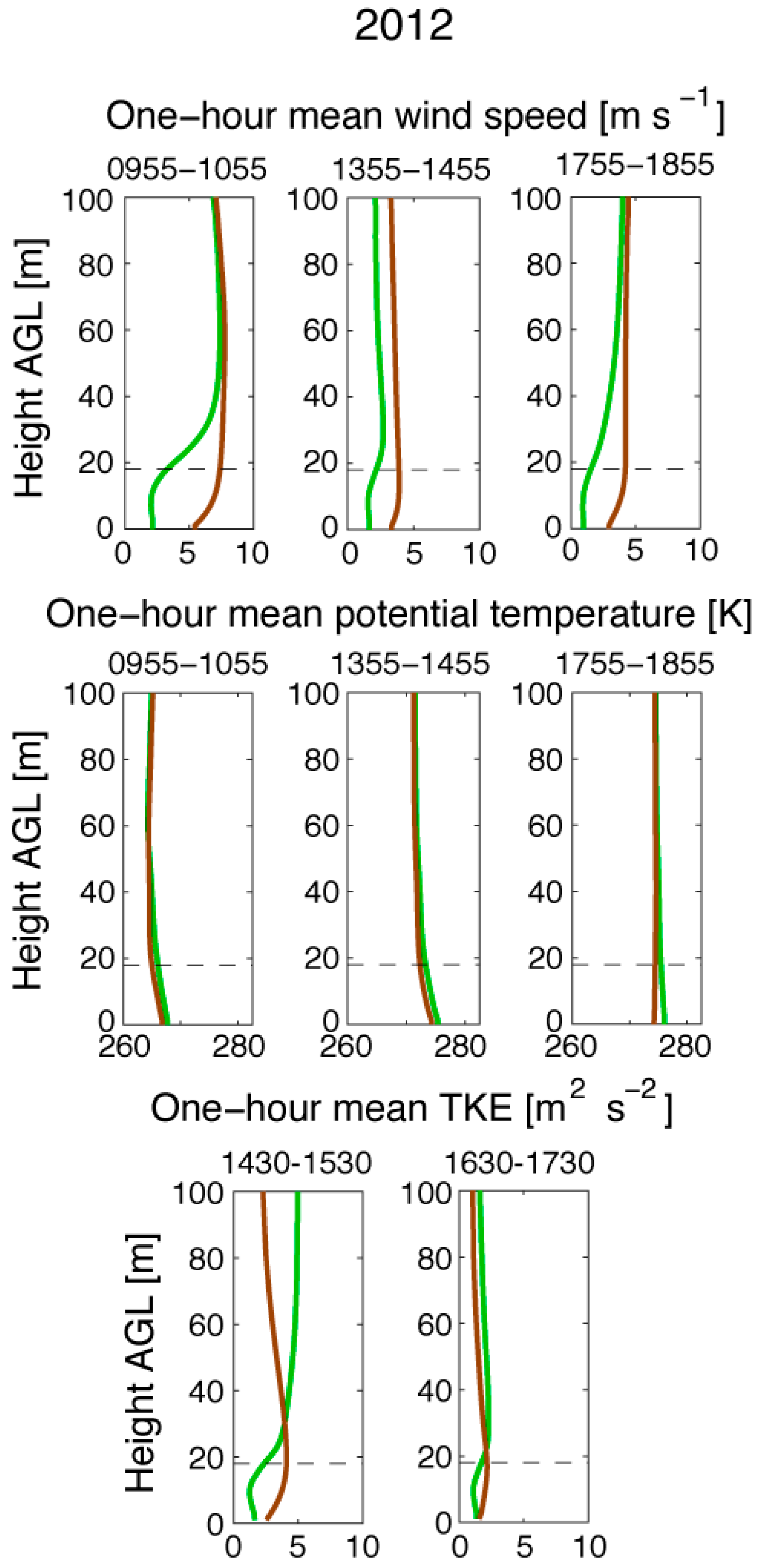
3.2.2. 2012 Case
4. Conclusions
Author Contributions
Funding
Acknowledgments
Conflicts of Interest
References
- Wildland Fire Executive Council. The National Strategy. The Final Phase in the Development of the National Cohesive Wildland Fire Management Strategy. Available online: http://www.forestsandrangelands.gov/strategy/documents/strategy/CSPhaseIIINationalStrategyApr2014.pdf (accessed on 13 May 2019).
- Larkin, N.K.; O’Neill, S.M.; Solomon, R.; Raffuse, S.; Strand, T.; Sullivan, D.C.; Krull, C.; Rorig, M.; Peterson, J.; Ferguson, S.A. The BlueSky smoke modeling framework. Int. J. Wildland Fire 2009, 18, 906–920. [Google Scholar] [CrossRef]
- Mell, W.E.; Manzello, S.L.; Maranghides, A.; Butry, D.; Rehm, R.G. The wildland–urban interface fire problem–current approaches and research needs. Int. J. Wildland Fire 2010, 19, 238–251. [Google Scholar] [CrossRef]
- Slaughter, J.C.; Koenig, J.Q.; Reinhardt, T.E. Association between lung function and exposure to smoke among firefighters at prescribed burns. J.Occup. Environ. Hyg. 2004, 1, 45–49. [Google Scholar] [CrossRef] [PubMed]
- Naeher, L.P.; Brauer, M.; Lipsett, M.; Zelikoff, J.T.; Simpson, C.D.; Koenig, J.Q.; Smith, K.R. Woodsmoke health effects: A review. Inhal. Toxicol. 2007, 19, 67–106. [Google Scholar] [CrossRef] [PubMed]
- Fernandes, P.M.; Botelho, H.S. A review of prescribed burning effectiveness in fire hazard reduction. Int. J. Wildland Fire 2003, 12, 117–128. [Google Scholar] [CrossRef]
- Edburg, S.L.; Allwine, G.; Lamb, B.; Stock, D.; Thistle, H.; Peterson, H.; Strom, B. A simple model to predict scalar dispersion within a successively thinned loblolly pine canopy. J. Appl. Meteorol. Clim. 2010, 49, 1913–1926. [Google Scholar] [CrossRef]
- Thistle, H.W.; Strom, B.; Strand, T.; Lamb, B.K.; Edburg, S.; Allwine, G.; Peterson, H.G. Atmospheric dispersion from a point source in four southern pine thinning scenarios: Basic relationships and case studies. Trans. ASABE 2011, 54, 1219–1236. [Google Scholar] [CrossRef]
- Kiefer, M.T.; Zhong, S.; Heilman, W.E.; Charney, J.J.; Bian, X. Evaluation of an ARPS-based canopy flow modeling system for use in future operational smoke prediction efforts. J. Geophys. Res. Atmos. 2013, 118, 6175–6188. [Google Scholar] [CrossRef]
- Maurer, K.D.; Bohrer, G.; Kenny, W.T.; Ivanov, V.Y. Large-eddy simulations of surface roughness parameter sensitivity to canopy-structure characteristics. Biogeosciences 2015, 12, 2533–2548. [Google Scholar] [CrossRef]
- Kiefer, M.T.; Heilman, W.E.; Zhong, S.; Charney, J.J.; Bian, X.; Skowronski, N.S.; Hom, J.L.; Clark, K.L.; Patterson, M.; Gallagher, M.R. Multiscale simulation of a prescribed fire event in the New Jersey Pine Barrens using ARPS-CANOPY. J. Appl. Meteorol. Clim. 2014, 53, 793–812. [Google Scholar] [CrossRef]
- Kiefer, M.T.; Heilman, W.E.; Zhong, S.; Charney, J.J.; Bian, X. Mean and Turbulent Flow Downstream of a Low-Intensity Fire: Influence of Canopy and Background Atmospheric Conditions. J. Appl. Meteorol. Clim. 2015, 54, 42–57. [Google Scholar] [CrossRef]
- Goodrick, S.L.; Achtemeier, G.L.; Larkin, N.K.; Liu, Y.; Strand, T.M. Modelling smoke transport from wildland fires: A review. Int. J. Wildland Fire 2013, 22, 83–94. [Google Scholar] [CrossRef]
- Brioude, J.; Arnold, D.; Stohl, A.; Cassiani, M.; Morton, D.; Seibert, P.; Angevine, W.; Evan, S.; Dingwell, A.; Fast, J.D.; et al. The Lagrangian particle dispersion model FLEXPART-WRF version 3.1. Geosci. Model Dev. 2013, 6, 1889–1904. [Google Scholar] [CrossRef]
- Stohl, A.; Forster, C.; Frank, A.; Seibert, P.; Wotawa, G. Technical note: The Lagrangian particle dispersion model FLEXPART version 6.2. Atmos. Chem. Phys. 2005, 5, 2461–2474. [Google Scholar] [CrossRef]
- Byun, D.W.; Ching, J. Science Algorithms of the EPA Model-3 Community Multiscale Air Quality (CMAQ) Modeling System; National Sxposure Research Laboratory, EPA: Washington, DC, USA, 1999.
- Solomos, S.; Amiridis, V.; Zanis, P.; Gerasopoulos, E.; Sofiou, F.I.; Herekakis, T.; Brioude, J.; Stohl, A.; Kahn, R.A.; Kontoes, C. Smoke dispersion modeling over complex terrain using high resolution meteorological data and satellite observations–The FireHub platform. Atmos. Environ. 2015, 119, 348–361. [Google Scholar] [CrossRef]
- Kontoes, C.; Solomos, S.; Amiridis, V.; Herekakis, T. Synergistic Satellite and Modeling Methods for the Description of Biomass Smoke Dispersion Over Complex Terrain. In Perspectives on Atmospheric Sciences; Springer: Cham, Switzerland, 2017; pp. 809–815. [Google Scholar]
- Solomos, S.; Gialitaki, A.; Marinou, E.; Proestakis, E.; Amiridis, V.; Baars, H.; Komppula, M.; Ansmann, A. Modeling and remote sensing of an indirect Pyro-Cb formation and biomass transport from Portugal wildfires towards Europe. Atmos. Environ. 2019, 206, 303–315. [Google Scholar] [CrossRef]
- Heilman, W.E.; Zhong, S.; Hom, J.L.; Charney, J.J.; Kiefer, M.T.; Clark, K.L.; Skowronski, N.S.; Bohrer, G.; Lu, W.; Liu, Y.; et al. Development of Modeling Tools for Predicting Smoke Dispersion from Low-Intensity Fires. Available online: https://www.firescience.gov/projects/09-1-04-1/project/09-1-04-1_final_report.pdf (accessed on 13 May 2019).
- Heilman, W.E.; Clements, C.B.; Seto, D.; Bian, X.; Clark, K.L.; Skowronski, N.S.; Hom, J.L. Observations of fire-induced turbulence regimes during low-intensity wildland fires in forested environments: Implications for smoke dispersion. Atmos. Sci. Lett. 2015, 16, 453–460. [Google Scholar] [CrossRef]
- Heilman, W.E.; Bian, X.; Clark, K.L.; Skowronski, N.S.; Hom, J.L. Atmospheric turbulence observations in the vicinity of surface fires in forested environments. J. Appl. Meteorol. Clim. 2017, 56, 3133–3150. [Google Scholar] [CrossRef]
- Byram, G.M. Combustion of Forest Fuels. Forest Fire: Control and Use, 1st ed.; Davis, K.P., Ed.; McGraw-Hill: New York, NY, USA, 1959; pp. 61–89. [Google Scholar]
- Xue, M.; Droegemeier, K.K.; Wong, V. The Advanced Regional Prediction System (ARPS)—A multi-scale nonhydrostatic atmosphere simulation and prediction model. Part I: Model dynamics and verification, Meteor. Atmos. Phys. 2000, 75, 161–193. [Google Scholar] [CrossRef]
- Xue, M.; Droegemeier, K.K.; Wong, V.; Shapiro, A.; Brewster, K.; Carr, F.; Weber, D.; Liu, Y.; Wang, D. The Advanced Regional Prediction System (ARPS)—A multi-scale nonhydrostatic atmosphere simulation and prediction tool. Part II: Model physics and applications, Meteor. Atmos. Phys. 2001, 76, 143–165. [Google Scholar] [CrossRef]
- Mesinger, F.G.; DiMego, E.; Kalnay, K.; Mitchell, P.C.; Shafran, W.; Ebisuzaki, D.; Jović, J.; Woollen, E.; Rogers, E.H.; Berbery, M.B.; et al. North American Regional Reanalysis. Bull. Am. Meteorol. Soc. 2006, 87, 343–360. [Google Scholar] [CrossRef]
- Wei, M.; Toth, Z.; Wobus, R.; Zhu, Y. Initial perturbations based on the ensemble transform (ET) technique in the NCEP global operations forecast system. Tellus A 2008, 60, 62–79. [Google Scholar] [CrossRef]
- The ARPS System. Available online: http://www.caps.ou.edu/ARPS/arpsdown.html (accessed on 13 May 2019).
- Skowronski, N.S.; Clark, K.L.; Duveneck, M.; Hom, J.L. Three-dimensional canopy fuel loading predicted using upward and downward sensing LiDAR systems. Remote Sens. Environ. 2011, 115, 703–714. [Google Scholar] [CrossRef]
- Sun, R.; Jenkins, M.A.; Krueger, S.K.; Mell, W.; Charney, J.J. An evaluation of fire-plume properties simulated with the Fire Dynamics Simulator (FDS) and the Clark coupled wildfire model. Can. J. For. Res. 2006, 36, 2894–2908. [Google Scholar] [CrossRef]
- Powers, J.G.; Klemp, J.B.; Skamarock, W.C.; Davis, C.A.; Dudhia, J.; Gill, D.O.; Coen, J.L.; Gochis, D.J. The Weather Research and Forecasting (WRF) Model: Overview, System Efforts, and Future Directions. Bull. Am. Meteorol. Soc. 2017, 98, 1717–1737. [Google Scholar] [CrossRef]
- Hanna, S.R. Applications in air pollution modeling. In Atmospheric Turbulence and Air Pollution Modeling; Nieuwstadt, F.T.M., van Dop, H.D., Eds.; Reidel Publishing Company: Dordrecht, Holland, 1982; pp. 275–310. [Google Scholar]
- Anderson, G.K.; Sandberg, D.V.; Norheim, R.A. Fire Emission Production Simulator (FEPS) User’s Guide, U.S. Forest Service. Available online: http://www.fs.fed.us/pnw/fera/feps/FEPS_users_guide.pdf (accessed on 13 May 2019).
- Liu, Y.; Goodrick, S.L.; Achtemeier, G.L.; Forbus, K.; Combs, D. Smoke plume height measurement of prescribed burns in the southeastern United States. Int. J. Wildland Fire 2013, 22, 130–147. [Google Scholar] [CrossRef]


© 2019 by the authors. Licensee MDPI, Basel, Switzerland. This article is an open access article distributed under the terms and conditions of the Creative Commons Attribution (CC BY) license (http://creativecommons.org/licenses/by/4.0/).
Share and Cite
Charney, J.J.; Kiefer, M.T.; Zhong, S.; Heilman, W.E.; Nikolic, J.; Bian, X.; Hom, J.L.; Clark, K.L.; Skowronski, N.S.; Gallagher, M.R.; et al. Assessing Forest Canopy Impacts on Smoke Concentrations Using a Coupled Numerical Model. Atmosphere 2019, 10, 273. https://doi.org/10.3390/atmos10050273
Charney JJ, Kiefer MT, Zhong S, Heilman WE, Nikolic J, Bian X, Hom JL, Clark KL, Skowronski NS, Gallagher MR, et al. Assessing Forest Canopy Impacts on Smoke Concentrations Using a Coupled Numerical Model. Atmosphere. 2019; 10(5):273. https://doi.org/10.3390/atmos10050273
Chicago/Turabian StyleCharney, Joseph J., Michael T. Kiefer, Shiyuan Zhong, Warren E. Heilman, Jovanka Nikolic, Xindi Bian, John L. Hom, Kenneth L. Clark, Nicholas S. Skowronski, Michael R. Gallagher, and et al. 2019. "Assessing Forest Canopy Impacts on Smoke Concentrations Using a Coupled Numerical Model" Atmosphere 10, no. 5: 273. https://doi.org/10.3390/atmos10050273
APA StyleCharney, J. J., Kiefer, M. T., Zhong, S., Heilman, W. E., Nikolic, J., Bian, X., Hom, J. L., Clark, K. L., Skowronski, N. S., Gallagher, M. R., Patterson, M., Liu, Y., & Hawley, C. (2019). Assessing Forest Canopy Impacts on Smoke Concentrations Using a Coupled Numerical Model. Atmosphere, 10(5), 273. https://doi.org/10.3390/atmos10050273