Article

Climate Change Projections of Extreme Temperatures for the Iberian Peninsula

Department of Physics and Centre for Environmental and Marine Studies (CESAM)–University of Aveiro, Campus Universitário de Santiago, 3810-093 Aveiro, Portugal
*
Author to whom correspondence should be addressed.
Atmosphere 2019, 10(5), 229; https://doi.org/10.3390/atmos10050229
Submission received: 26 March 2019 / Revised: 16 April 2019 / Accepted: 26 April 2019 / Published: 29 April 2019
(This article belongs to the Section Meteorology)

Abstract

:
The comprehensive characterization of heat waves and extreme hot days is fundamental for policymakers due to its vast implications for human health. This study evaluates extreme temperature changes over the Iberian Peninsula for the present climate and future projections, considering extreme temperature indices, cold/heat waves, and a recovery factor, using the Weather Research and Forecasting model. The projected temperatures show an increase of over 6 °C. An increase in the number of summer days and tropical nights and a decrease in frost days is expected. The number of heat waves and their duration and intensity are expected to increase. The number of heat wave days are expected to increase, with much of the average summer season being under heat wave conditions. The recovery factor is expected to decrease. Cold spells are projected to decrease in terms of number, intensity, duration, and number of spell days, whereas the recovery factor is expected to increase. Heat wave analysis was combined with maximum temperature thresholds to isolate extreme heat waves. The results show an increase in extreme heat wave days, with regions experiencing over 10 heat wave days with maximum temperature surpassing 45 °C for the long-term future.

Graphical Abstract

1. Introduction

Climate change is one of the major threats of the 21st century. The main concern with the evaluation of climate change impacts is the associated potential change in climate variability and, consequently, in extreme events [1]. Extreme events are defined as the tails of the distribution of a weather variable, which occur with low frequency, that is, the values located away from the mean or median value of the distribution [2]. Examples are extreme temperature events (heat waves, cold spells, and the number of days exceeding different threshold temperatures) and extreme precipitation events (heavy rain and droughts). These events are responsible for significant impacts on both human society and the natural environment, for instance, human morbidity/mortality and economic losses [3,4]. Several studies point to an increase in the frequency of extreme events associated with an increase in temperature [3,5,6].
Regional climate models (RCMs), such as the Weather Research and Forecasting model (WRF), are frequently used to provide detailed information on extremes and not only on average conditions [6]. Generally, global climate models (GCMs) are used as forcing models to RCMs, providing information about the initial and boundary conditions. However, this combination of GCMs and RCMs, often introduces systematic errors in the simulations [7,8,9], which might be amplified when studying extreme events such as extreme temperatures [10].
Models are simplifications of reality, and therefore, there are small differences between the statistics of the observations and the climate model simulation. These differences are called biases or systematic errors. These biases can be due to simplified physics and thermodynamic processes, mathematical formulation of the numerical integrations, limited knowledge of the climate system process, and limited spatial resolution in the climate model.
With the purpose of reducing such systematic errors, several studies have applied bias correction methods to RCM simulations [9,11,12,13]. These authors used quantile mapping as a method of correction, with improved results for temperature. Different methodologies have been developed in order to reduce the model biases, for instance, the quantile mapping, which is applied in this study.
Numerous studies have focused on observed and simulated historical and future changes in extreme temperature events [6,14,15,16], considering the exceedance of a fixed absolute value or the deviation from the historical climatology, using the maximum and minimum temperature, climate change indices, or heat waves and cold spells. In the future, a pronounced warming in the Mediterranean is projected, mainly during summer and in maximum temperature [5,17]. Consequently, an increase in the indices associated with hot extremes is estimated, conversely, with a decrease in the ones associated with cold events [18,19]. An increase in the frequency of the heat waves and a decrease in the cold spells in the Iberian Peninsula is also projected [20].
Nowadays, climate change with respect to extreme temperatures is a well-recognized problem. Ongoing effects of heat waves and extreme hot days include consequences on human morbidity/mortality and on the environment and economy [3,21]. These impacts are even more pronounced in urban areas with high population density, which are heavily vulnerable to extreme temperature events. Thus, assessing this type of event is crucial during the policymaking process, when both mitigation and adaptation measurements are addressed.
The main purpose of this study is to evaluate the change in extreme temperatures in the Iberian Peninsula for two future climate periods relative to a historical recent climate. This is done using a set of climate simulations performed by WRF RCM and forced by the Max Planck Institute earth system model–low resolution (MPI-ESM-LR) GCM. First, because the modeling of climate may have systematic errors, bias correction was applied to the simulations using a quantile mapping approach. The change in extreme temperature was evaluated through the differences between the future climates and the historical climate and respective statistical significance, combining the maximum and minimum temperature, climate change indices, heat waves and cold spells characteristics, and their recovery factor.
The novelty of this study is that it considers many complementary aspects of temperature relevant to thermal stress, bias correction is performed prior to the climate change analysis, and the statistical significance of changes is evaluated.
The article is structured as follows: in Section 2, we describe the data and methods used, where we detail the bias correction approach used in this study, the variables used to evaluate the climate change—climate change indices, heat waves and cold spells—and their formulation. Afterwards, in Section 3, we present and discuss the results obtained, referring to the model validation and future change in extreme temperatures. In Section 4, we present a summary with our conclusions.

2. Data and Methods

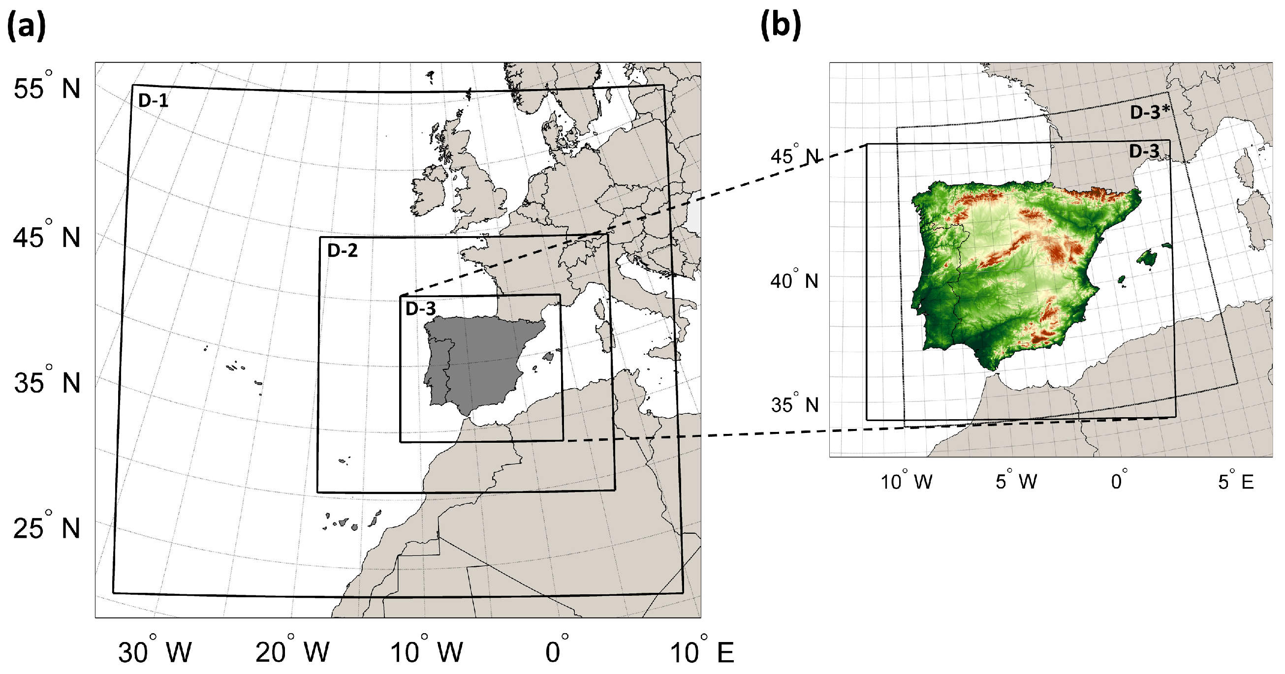
2.1. Data and Simulations

For this study, a set of WRF v3.5 (Weather Research and Forecasting) simulations, previously performed and validated, were used [22]. The WRF model is a numerical weather prediction (NWP) system developed for both research and operational applications.
The WRF model is a fully compressible, non-hydrostatic, primitive-equation model with multiple nesting capabilities and variable time integration [23]. It is a very versatile numerical model used to simulate storms [24], heavy rainfall events [25], and urban heat island [26]. Moreover, it has been successfully used as a regional climate model [22,27,28,29].
WRF simulations were driven by the global climate model MPI-ESM-LR (WRF-MPI), which provided the initial and boundary conditions to obtain regional climate information through a method called dynamical downscaling. This process takes information from larger scales to the local/regional scale.
The MPI model with r1i1p1 initialization has a horizontal resolution of 1.9°, which corresponds to about 160 km [30]. For these simulations, WRF-MPI was set with 29 vertical levels defined as eta-terrain-following coordinates, unevenly spaced with a higher resolution directly over the surface to better capture the boundary layer representation. Several different physical parameterizations using the WRF model were tested for the Iberian Peninsula [31]. Their results are used in this study. The physical parametrizations used include WRF single-moment 6-class microphysical scheme [32], Dudhia shortwave radiation scheme [33], RRTMG (rapid radiative transfer model) longwave radiation model [34], MM5 similarity surface layer scheme [35], Noah land surface model [36], Yonsei University planetary boundary layer scheme [32], and Grell–Freitas ensemble scheme for cumulus parametrization [37]. Because model simulations are sensible to land use, the Coordination of Information on the Environment (CORINE) Land Cover was implemented [38]. The process consisted of converting CORINE data categories into WRF categories [39]. Sensitivity tests were performed for the usage of this dataset in WRF simulations [40].
The model was integrated without interruption for 21 years for the three periods. This extra starting year is the spin-up year necessary to allow the soil moisture to adjust [22]. In this study, the boundary conditions from MPI were provided to WRF at six-hour intervals, including the sea surface temperature. To avoid mismatches between MPI boundaries and WRF, all simulations were performed using spectral nudge for wavelengths larger than 1000 km [41].
To make WRF outputs more resembling a climate simulation, in the sense that climate simulations are concerned with averages, sums, and minimum and maximum values, a set of modifications were introduced allowing for output of the daily minimum and maximum temperature [29]. In doing so, it was ensured that the minimum and maximum fell in daily intervals.
The MPI model participated in the Coupled Model Intercomparison Project Phase 5 (CMIP5) [42], which uses new emission scenarios, namely the representative concentration pathways (RCPs) [19].
This study comprises two future periods—medium- (2046–2065) and long-term (2081–2100)—and a historical period (1986–2005). These simulations were performed for 20-year periods, as used by the Intergovernmental Panel on Climate Change (IPCC) 5th Assessment Report [43]. The future simulations consider a future greenhouse gas emission scenario, namely RCP8.5, defined by a radiative forcing of 8.5 W m−2 by 2100 and a continuous increase after this year [44]. Several studies have used this forcing model as the key driver for future climate change estimation [14,20,45,46,47].
The WRF-MPI model was implemented for three two-way nested domains with an increasing horizontal resolution, using a fixed nesting ratio of three, namely 81, 27, and 9 km. This study focuses on the innermost domain, with higher resolution (9 km, D-3), which includes the Iberian Peninsula (Figure 1a).
Bias correction was applied to the original simulations using observational data as a reference. These observational data—E-OBS—developed by the European Climate Assessment and Dataset (ECA&D), consist of a land-only, daily, high-resolution gridded dataset for Europe, which cover a period between 1950 and 2006 [48]. These data comprise precipitation and minimum, maximum, and mean surface temperature. In this study, we extracted the daily minimum and maximum temperature for an interval equal to the historical period of the simulations—1986–2005—for a rotated pole grid with a horizontal resolution of 0.22°.
A regular grid with a horizontal resolution of 0.2° was defined (D-3*) (Figure 1b), which allows for the comparison between the simulations and the observational data.
Past research shows that there are breaks in the homogeneity of the temperature and within the temperature data. The inhomogeneities are more significant in the day-to-day difference in temperature than in the daily amplitude [49]. This information may be important when calculating trends using E-OBS. Regardless, it was shown that E-OBS satisfactorily reproduced temperature data and indices in most study sites, despite the fact that precipitation indices were less accurate [50]. E-OBS succeeded in estimating trends in extreme temperature and precipitation.

2.2. Methods

Firstly, since the modeling of climate may have systematic errors, bias correction was applied to temperature simulations. The bias correction method applied in this study is explained in this section.
Afterwards, we focused on the change in extreme temperatures, which was evaluated by the mean differences of maximum and minimum temperature, climate change indices, heat waves, cold spells, and their recovery factor. Additionally, and not considered often in other similar studies, we evaluated the statistical significance of the changes of the future climates relative to the historical reference climate. The same test was applied to verify the differences between simulations, before and after bias correction, and the observations for the reference period. A two-tailed statistical hypothesis test—Student’s t-test—using a 5% significance level was applied [51,52].
The methods applied to calculate the climate change indices, heat waves, cold spells, and the recovery factor are detailed in this section.

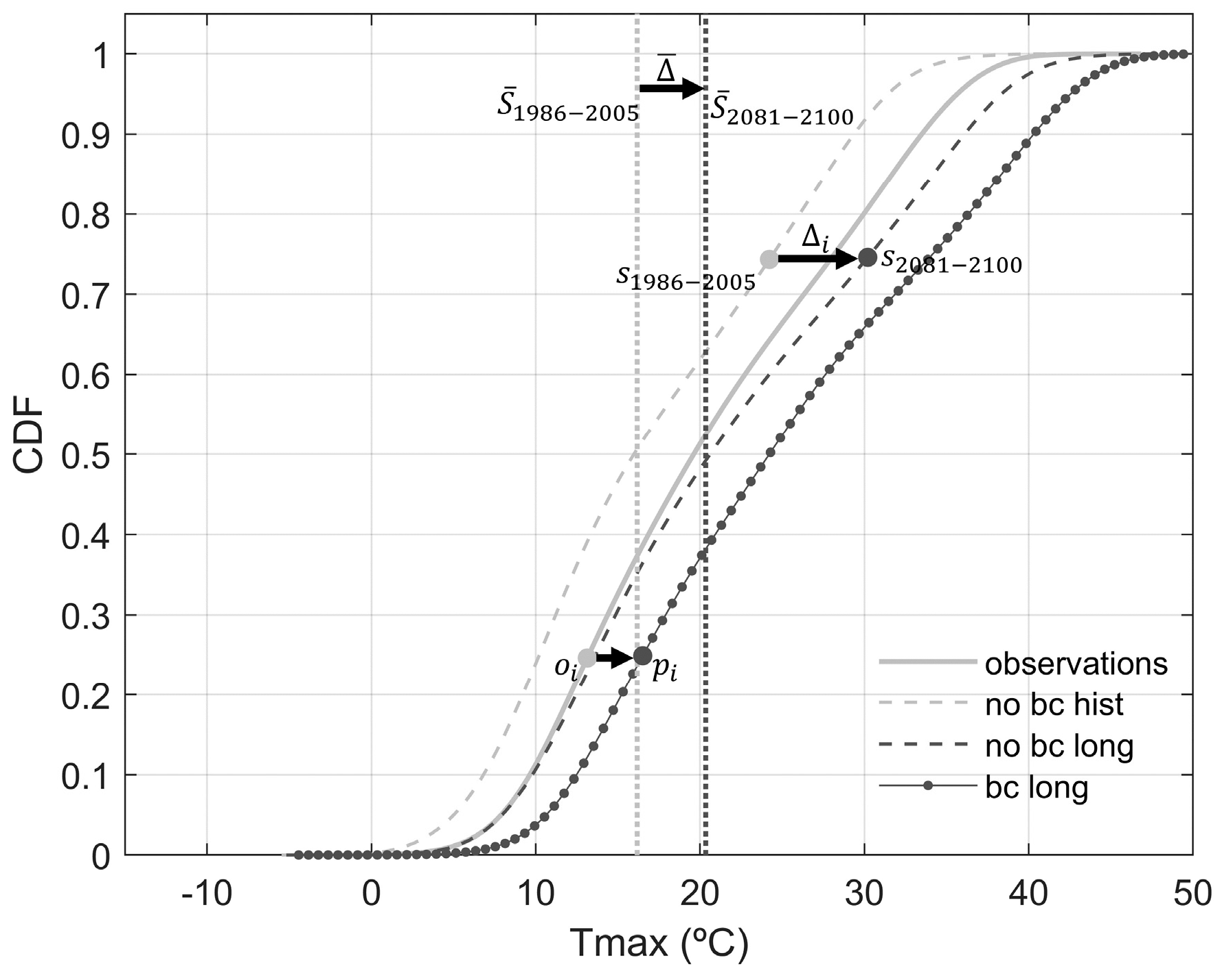
2.2.1. Bias Correction

The simulations performed by GCMs and RCMs frequently present systematic errors, triggered by low horizontal resolution, complex terrain, simplified parametrization of the thermodynamic and physical processes, or simplified numerical schemes [7,8,9]. With the purpose of minimizing the differences between simulated and observational data, numerous studies have applied bias correction to the simulations [9,53,54,55,56,57]. Bias correction of climate variables is a current issue and has been under debate since the correction may not preserve some characteristics of the variable. Thus, correcting climate variables is a balance between a reliable analysis and its possible side effects, with some authors presenting extensive discussions on the topic [58,59,60,61,62,63,64].
Some studies applied a quantile mapping bias adjustment method to reduce the model biases [11,12,13,65]. This approach consists of correcting the distribution individually for each quantile. For Europe, the results are controversial. Some mention that quantile mapping changes the indices based on thresholds [58]. On the other hand, some authors show that indices based on the duration of the event are affected [54]. Others present a detailed discussion about the error correction on climate variables, such as the temperature, and conclude that quantile mapping retains the quality of the temporal structure in the timeseries and the inter-variable dependencies of the regional climate models [66]. Despite the limitations, bias correction is commonly used to correct systematic distributional biases in climate variables such as temperature [67], and it is often considered more adequate than using raw simulated data.
In this study, we used a method that enables the minimization of the systematic errors verified in the daily maximum and minimum temperature simulations through a quantile–quantile calibration (q-q plot) [12]. This method assumes that the distribution function of the variable may change in the future. The advantage of this approach is the correction of the complete distribution including the tails, which, in this case, comprises the correction of extreme temperatures.
First, we performed bias correction of temperature for the historical period, by projecting the distribution of the observed temperature onto the simulated temperature for the historic period. Later, the temperatures in the future periods were also bias-corrected based on the method described briefly by the following equations, in which i corresponds to the i th ranked value of the respective cumulative distribution function (CDF) [12]:
i = s 2081 2100 s 1986 2005
¯ = i = 1 N i N =   S ¯ 2081 2100 S ¯ 1986 2005
i = i ¯
f = σ o σ S c = I Q R 75 25 | o I Q R 75 25 | S c
where s 2081 2100 is the future simulated temperature without bias correction for the long-term future case, s 1986 2005 is the historical temperature with no bias correction, and N is the number of days of the sample (in our study, N = 7670 ).
Therefore, Equation (1) represents the difference between the future and historical simulated temperature without bias correction. Equation (2) corresponds to the mean regime shift and Equation (3) to the deviations from this shift. Furthermore, Equation (4) represents the interquartile ranges of the observed and historical simulated temperature with no bias correction ( I Q R 75 25 | o and I Q R 75 25 | S c , respectively), which corresponds to the difference between the 75th and 25th percentiles. We assume the latter variables represent the variability of both observed and historical simulated temperature with no bias correction ( σ o and σ S c ) [12].
Thus, the future simulated temperatures with bias correction ( p i ) are calculated using the following equation [12], where o i is the observed temperature:
p i = o i + g ¯ + f i
where g and f are parameters that modulate the variation in the mean state and that calibrate the change in variability and shape, respectively. For temperature, we assume that the simulation shift in the mean is a plausible outcome of the models. Thus, this shift must be preserved in the projected simulations resulting in g = 1 .
The full methodology of the applied bias correction is presented by [12]. Bias correction was applied to the daily minimum and maximum temperature of each grid point of the domain. Figure 2 shows the application of the bias correction methodology to maximum temperature, performed on a single grid point representative of Madrid for only the long-term future. In this figure, an example of the shift from both historical and long-term future simulations is depicted before bias correction (in the 75th percentile) and their shift after applying bias correction to both simulations (25th percentile).

2.2.2. Climate Change Indices

The climate change indices, defined by the World Climate Research Programme’s Expert Team on Climate Change Detection and Indices (WCRP’s ETCCDI), consist of a set of 27 indices, which allow the quantification and characterization of the variability and change of climate [68,69]. This set of standard indices enables a consistent comparison between analyses performed by different authors and promotes the analysis of extremes all over the world. These have been used in several studies, which evaluate changes in extreme temperature [14,15,19,68,70], suggesting a very likely warming of the Iberian Peninsula.
Because this study focuses on extreme temperatures, we assessed three indices, which evaluate the changes in minimum and maximum temperatures, namely the number of summer days (SU25), number of frost days (FD0), and number of tropical nights (TR20).
The number of summer days is defined as the annual count of days in which maximum temperature is above 25 °C ( T m a x > 25   ° C ). The number of frost days considers days in which the minimum temperature is lower than 0 °C ( T m i n   < 0   ° C ). The number of tropical nights is defined as the annual number of days in which the minimum temperature is higher than 20 °C ( T m i n > 20   ° C ).

2.2.3. Heat Waves and Cold Spells

Several studies have evaluated the properties of heat waves and cold spells in historical and future climates [6,15,20,71,72,73]. In general terms, the results show surface warming [15] that may be related to a decrease in cold spells [20] and an increase in frequency, intensity, and duration of heat waves in Europe and in the Iberian Peninsula [6,20,71,72,73], with some models projecting an increase in the probability of occurrence of extreme and very extreme heat waves [20,71].
Different definitions are used to detect these events [74], which have a variable minimum number of consecutive days above a variable daily threshold. For instance, some authors define a heat wave as a minimum period of six consecutive days with maximum temperature exceeding its 90th percentile [6], while others consider a heat wave as a minimum of two consecutive days occurring above the 95th percentile of the daily maximum temperature [73]. Other studies consider different meteorological variables such as the relative humidity [74,75]. In addition, some studies use different methods to establish the daily threshold, namely the exceedance of a fixed absolute value or the deviation from normal [74].
In this study, we defined a heat wave (HW) using a methodology that considers a period of at least three consecutive days in which the maximum temperature is equal or superior to the daily threshold of the historical period (in our study, 1986–2005) [71]. Conversely, cold spells (CSs) are defined as an interval of at least three consecutive days with minimum temperature equal or inferior to the daily threshold of the historical period.
The daily threshold mentioned above has a different formulation for the heat waves and the cold spells. In the former case, it consists of the 90th percentile of the maximum daily temperature, while in the latter case it consists of the 10th percentile of the minimum daily temperature. Both daily thresholds for a particular day are calculated on a 31-day window centered on that day [20].
In this study, heat waves were only detected for summer for a period covering June to August (JJA), whereas cold spells were searched for winter, the period between December and February (DJF). With the aim of not restricting possible events occurring in the limits of these intervals, we counted three extra days in the beginning and in the end of the periods established.
To characterize the heat wave/cold spell events, we calculated the duration, intensity, waves’/spells’ number, and number of wave/spell days [20]. The intensity of a heat wave consists of the mean difference between the maximum temperature and the daily threshold, while the intensity of a cold spell considers the minimum temperature. Furthermore, we calculated the recovery factor, which is defined as the mean difference between the maximum and minimum temperature of the events (temperature range), representing the health recovering capacity during the night/day within a heat/cold wave/spell [20]. The characteristics of the heat waves and cold spells and the recovery factor are descripted in Table 1.
Due to the acknowledged increase in global temperatures, part of this study consisted of combining different thresholds of maximum temperature, namely 25 °C, 35 °C, 40 °C, and 45 °C, with the purpose of identifying very extreme heat waves in future climate scenarios. Thus, in this case, the daily threshold consisted of the combination of the exceedance of a fixed absolute value and the deviation from normal.

3. Results

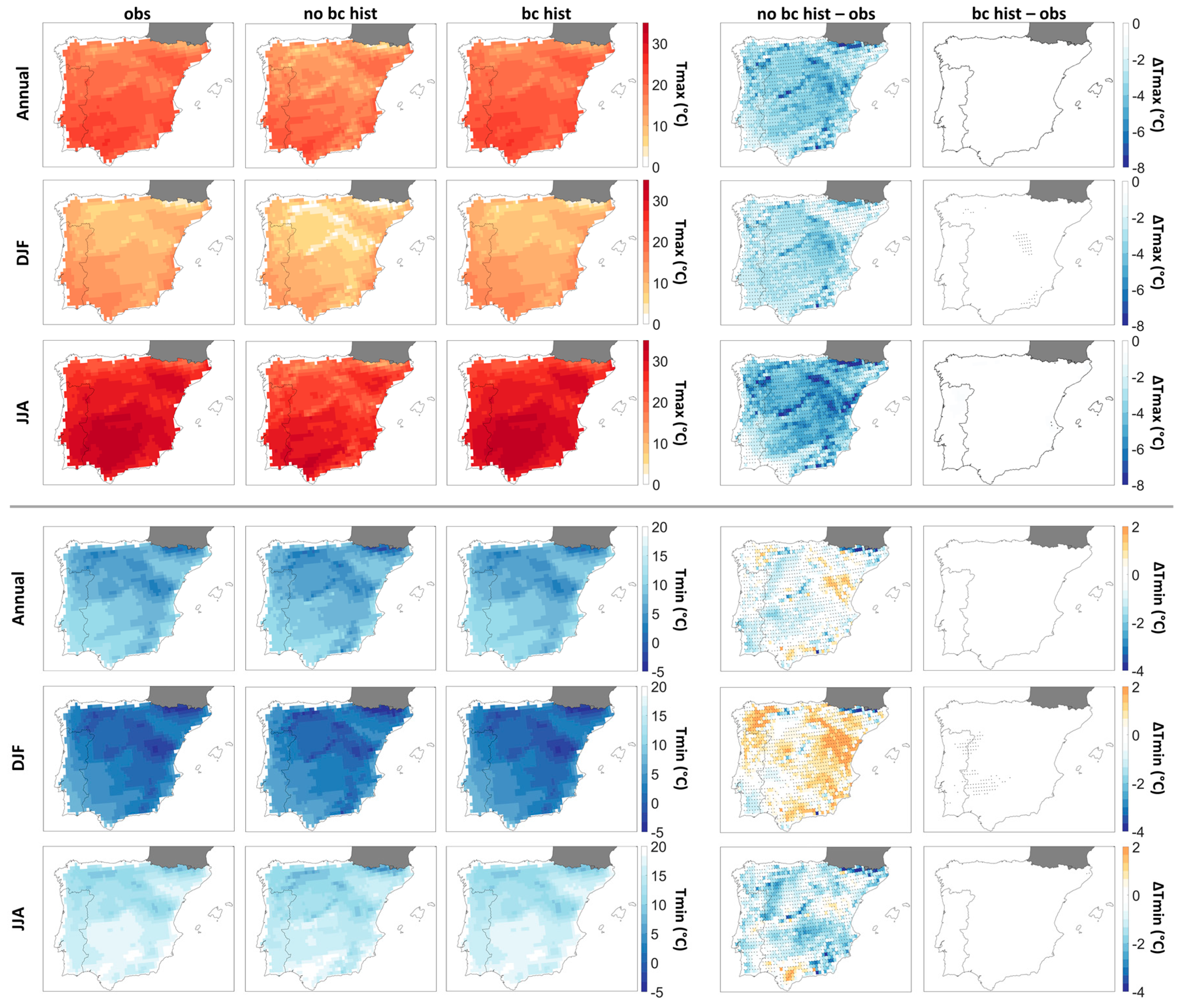
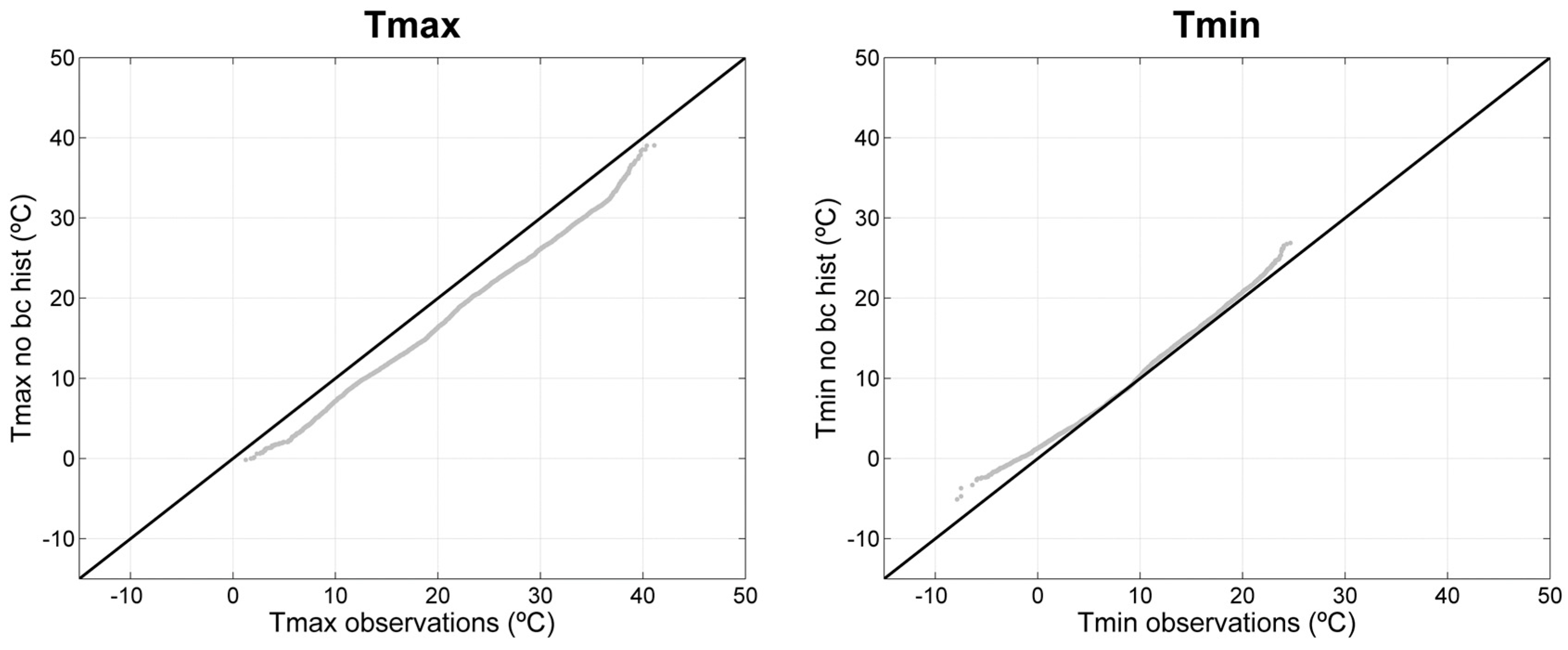
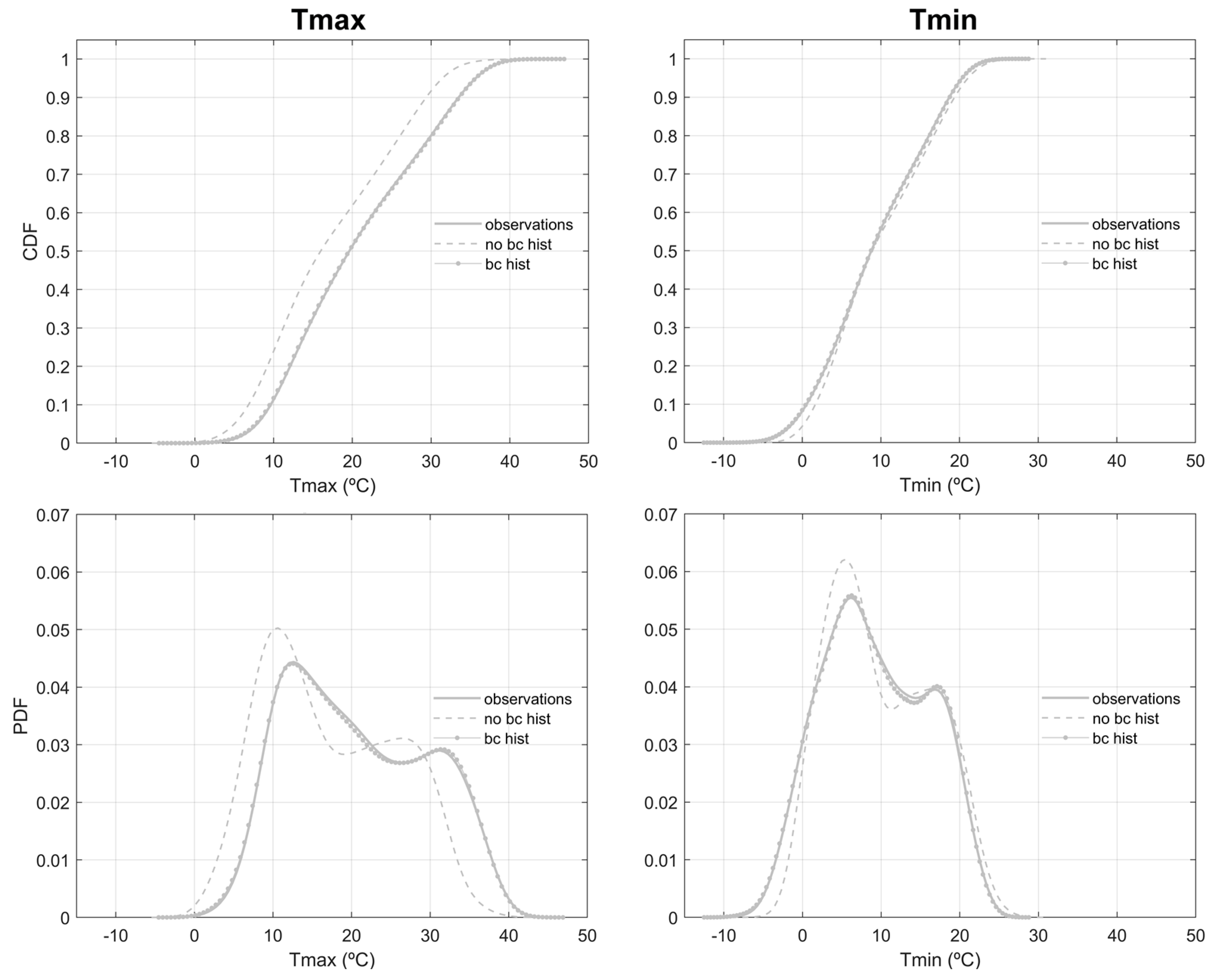
3.1. Model Validation

With the purpose of validating the bias correction applied to the maximum and minimum temperature simulated by WRF-MPI, we compared the observations (E-OBS) with the historical simulations with and without bias correction.
First, we calculated the mean spatial distribution of the observations (obs) and the simulations from the historical period with and without bias correction (bc hist and no bc hist, respectively), their differences, and respective statistical significance (Figure 3). All calculations were performed considering annual and seasonal mean fields (summer—JJA and winter—DJF).
Before bias correction, the maximum temperature is underestimated relative to the observations. These differences are statistically significant, and their peak occurs in regions with higher altitude and during summer. After applying the bias correction, these differences are approximately null and statistically non-significant (Figure 3). The minimum temperature is underestimated and overestimated by the WRF-MPI simulations in different regions of the domain. These statistically significant differences are predominantly positive during winter and negative during summer. After bias correction, the differences became approximately null and statistically non-significant, with the exception of a small region in the central Iberian Peninsula (Figure 3).
For a better understanding of the bias correction method applied, Figure 4 shows the quantile–quantile plots of the maximum and minimum temperature observed and simulated for the historical period with and without bias correction for a grid point representative of Madrid. The quantiles of the simulated maximum temperature presented lower temperatures than those observed. On contrary, the simulated minimum temperature adjusted to the observations with the exception of the extremes of the distribution, where an overestimation of the temperature was verified mainly in the lower temperatures (DJF). Similar results have been verified in Figure 3.
Figure 5 represents the CDF and the probability density function (PDF) of maximum and minimum temperature simulated for the historical period with and without bias correction and that observed for Madrid. It is important to notice that, after bias correction, the simulated temperature for the historical period and the observations were similar.
The CFD and PDF of maximum temperature with no bias correction were shifted in the direction of the lower temperatures, when compared to the observations. The CDF and PDF representatives of the minimum temperature were similar, with the exception of the extremes, where a shift of the distribution with no bias correction in the direction of the higher temperatures can be observed mainly in the lower temperatures (DJF). Similar results can be observed in Figure 3 and Figure 4.
Analyzing Figure 3, Figure 4 and Figure 5, we verified model temperature biases for minimum and maximum temperatures. After the application of the bias correction, both simulations and observations were similar. Thus, the model was validated with success, and, hereafter only bias-corrected temperature will be used.

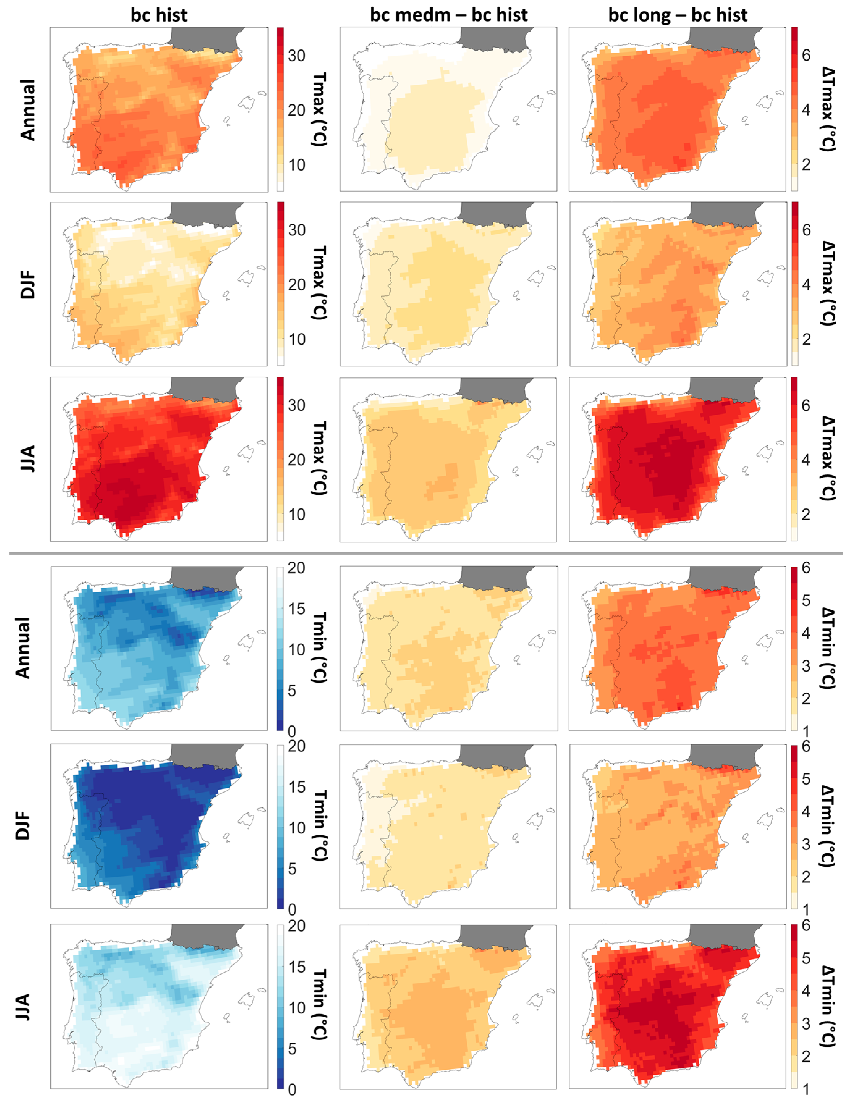
3.2. Future Change in Extreme Temperatures

To evaluate the change in extreme temperature, we focused on the differences between the future climate scenarios and the historical period and respective statistical significance. We combined maximum and minimum temperature, climate change indices, heat waves/cold spells’ properties and the associated recovery factor, and a combination of daily maximum temperature thresholds and heat waves.

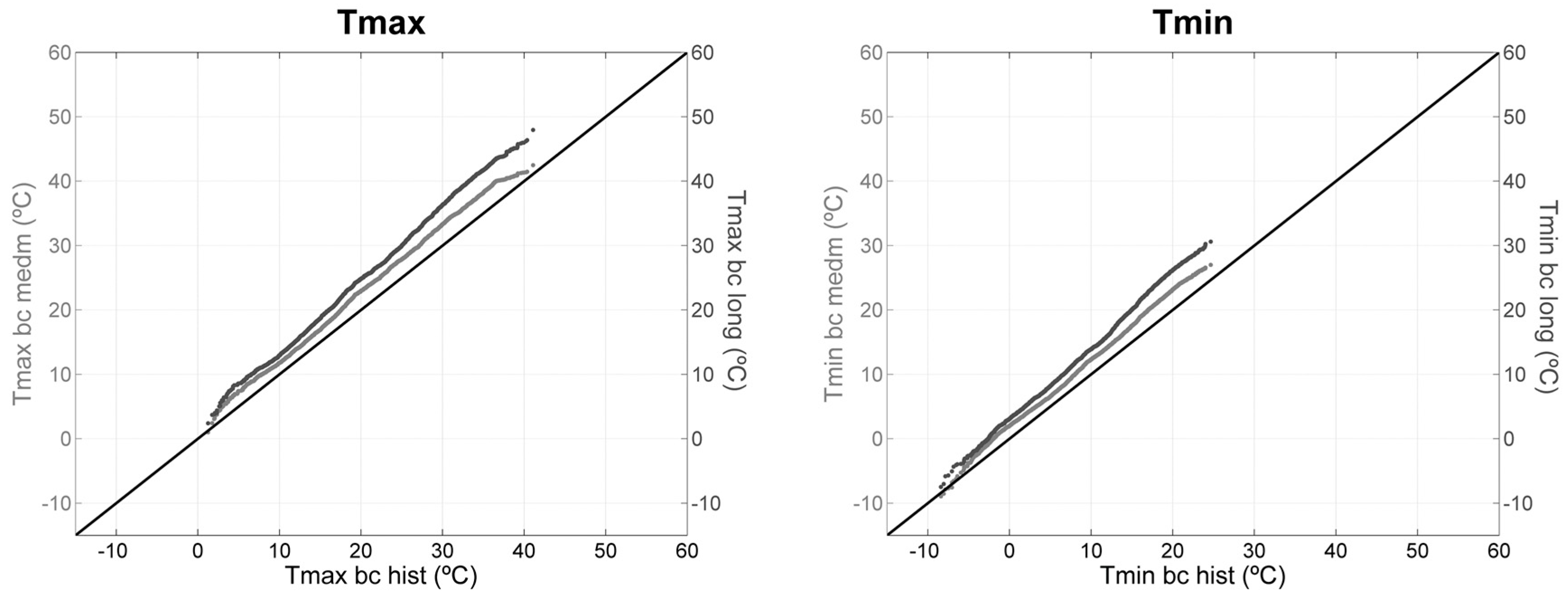
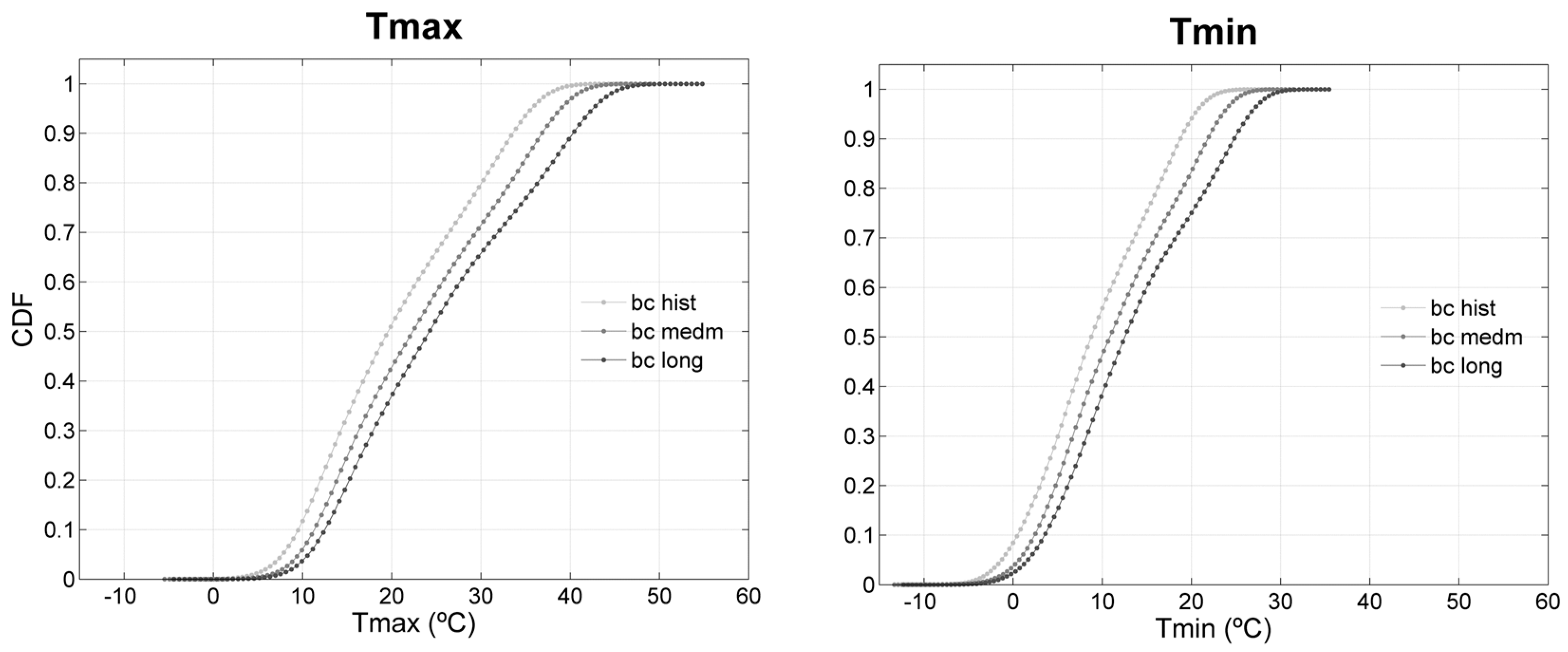
3.2.1. Maximum and Minimum Temperature

First, we calculated the mean spatial distribution of the maximum and minimum temperature for the historical climate and the differences between the future and historical periods. Figure 6 shows a future increase in temperature, which is more pronounced for maximum temperature during summer. For the medium- and long-term future, a significant increase in the annual minimum and maximum temperature, greater than 2 °C and 4 °C respectively, is expected, although during summer, the increase in both minimum and maximum temperature might be superior to 6 °C. These changes are statistically significant over the whole domain. This pronounced warming during summer has been verified in previous studies [17,76], while others noticed the pronounced increase in maximum temperature [5,19,77].
In the scope of CMIP5, several studies have evaluated the performance of several models (including MPI-ESM-LR) in simulating past and future extreme temperatures in Europe. A study was performed using 33 global climate models participating in CMIP5, under the RCP8.5 [78]. For the climate change analysis, the ensemble-mean temperatures are expected to increase over all of Europe during winter and summer. Focusing on the Iberian Peninsula, a warming between 2 and 4 °C is projected during winter. For summer, the temperature is likely to increase between 5–7 °C, with a more pronounced increase in central Iberian Peninsula. The results are similar to the ones presented by our study, which also show a more pronounced increase in temperature during summer and in the innermost region of the Peninsula.
For a better understanding of future changes of temperature’s distribution, Figure 7 shows quantile–quantile plots of the maximum and minimum temperature simulated for the historical and both future periods for Madrid. The quantiles that are representative of both maximum and minimum temperatures have the same behavior.
The quantiles of the historical period have lower temperatures than those in the future periods, associated with a future increase in temperature. However, these differences are enhanced in the maximum temperature range, which is also shown in Figure 6. Furthermore, the increase in temperature in the medium-term future is lower than that observed in the long-term future, although the differences between both future periods are more pronounced for higher values of temperature, which is associated with an unequal warming of the different quantiles. Thus, the higher the temperature during the historical period, the greater the increase in temperature in the future periods. The higher (lower) temperatures of both minimum and maximum temperature are most likely associated with summer (winter), in which a more (less) pronounced increase in temperature was previously observed (Figure 6).
Figure 8 represents the CDF of the maximum and minimum temperature simulated for the historical and future periods for Madrid. Their behavior is similar to that observed in Figure 7. Thus, both future periods are shifted in the direction of the higher temperatures, especially in the maximum temperature. In addition, the increase in temperature in the medium-term future is lower than that observed in the long-term future. Finally, the higher the temperature during the historical period, the greater the increase in temperature in the future. Therefore, in the future, a greater increase in temperature for higher temperature extremes (high maximum and minimum temperature) is expected than for lower temperature extremes.

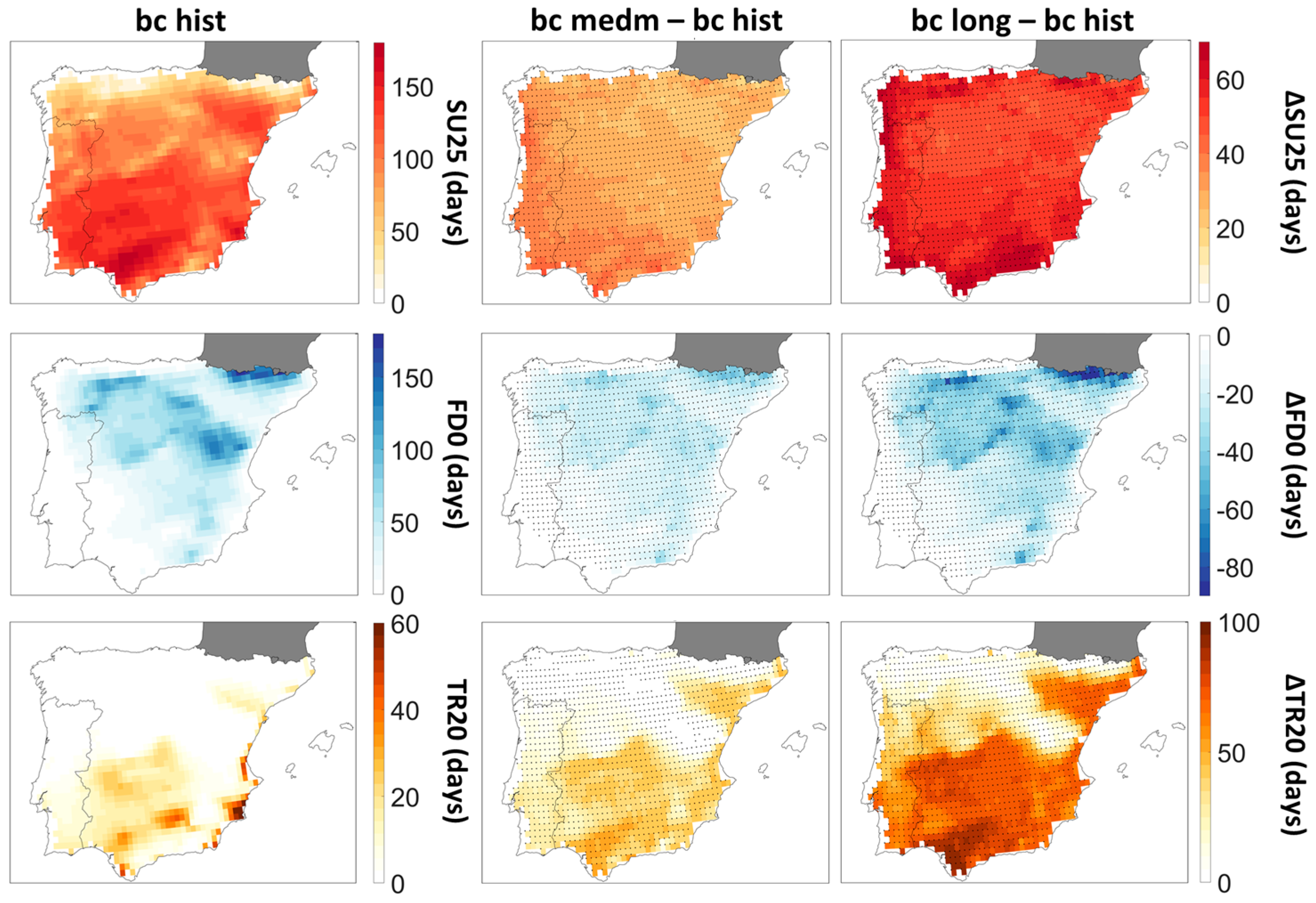
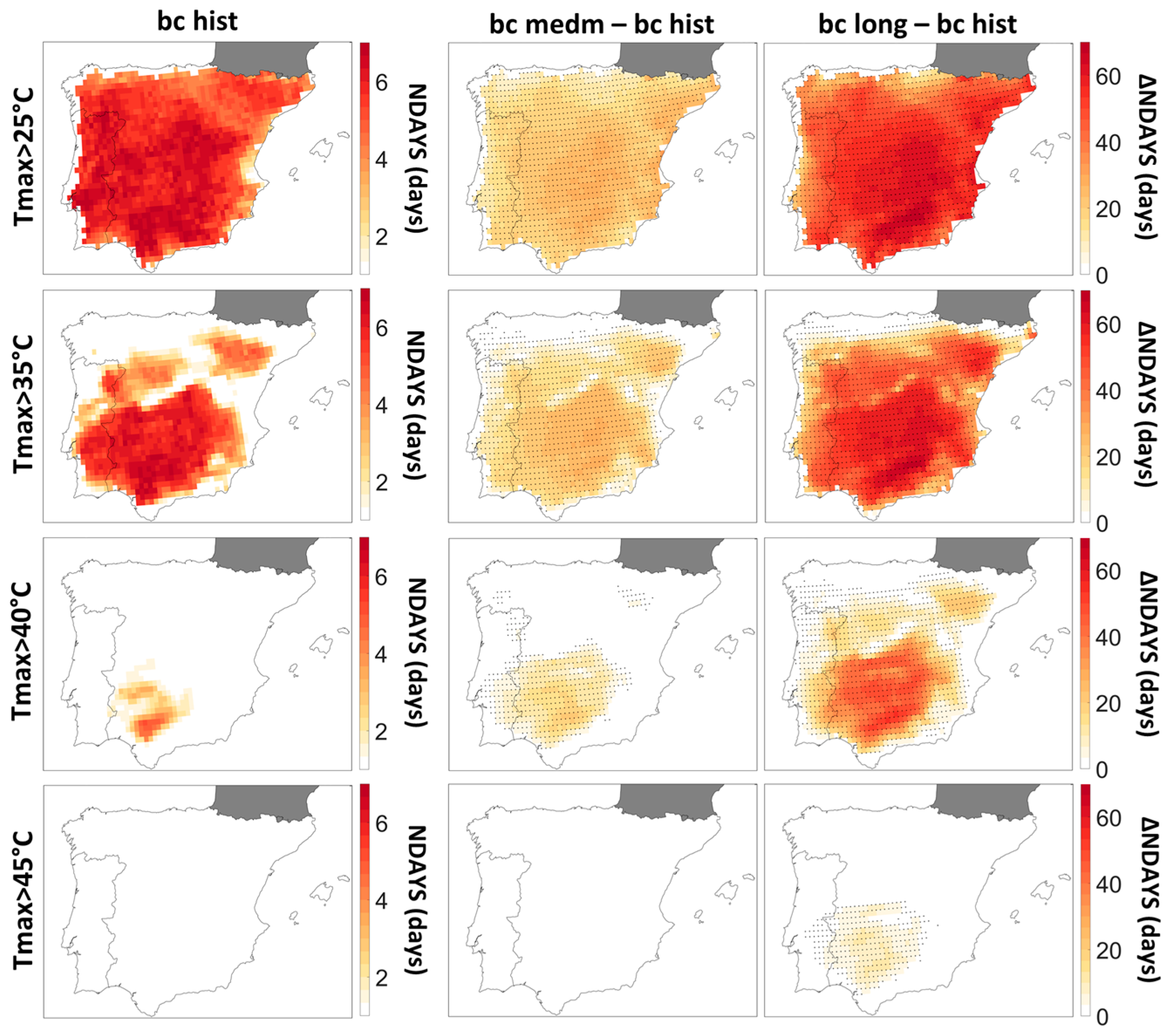
3.2.2. Climate Change Indices

To further evaluate temperature changes, other independent and universally adopted methods have been used here, namely changes in some of the ETCCDI indices. As said before, these are the number of summer days (SU25), number of frost days (FD0), and number of tropical nights (TR20). Figure 9 shows the spatial distribution of these mean indices for the historical climate and the differences between the future and historic climates. The statistical significance of these changes has also been assessed.
In the future, a statistically significant increase of the SU25 is expected, when compared with the historical period. In the medium-term future, this increase is around one month, while for the long-term future it is approximately two months. In addition, in the future, a statistically significant decrease in the number of FD0 is estimated. In the historical period, some areas in the southwest region of the domain do not have frost days. However, in the future, in which a decrease of 80 days is estimated in certain areas, the area with no frost days is expected to increase. Finally, in the future, a significant increase in the number of TR20 is estimated, with more than 100 nights (greater than 3 months) in the long-term future for much of the southern part of the domain. Statistically significant changes are observed over most of the domain.
Previous studies have also shown similar recent and future positive trends to those presented here [14,15,18,19,70,77,79,80].

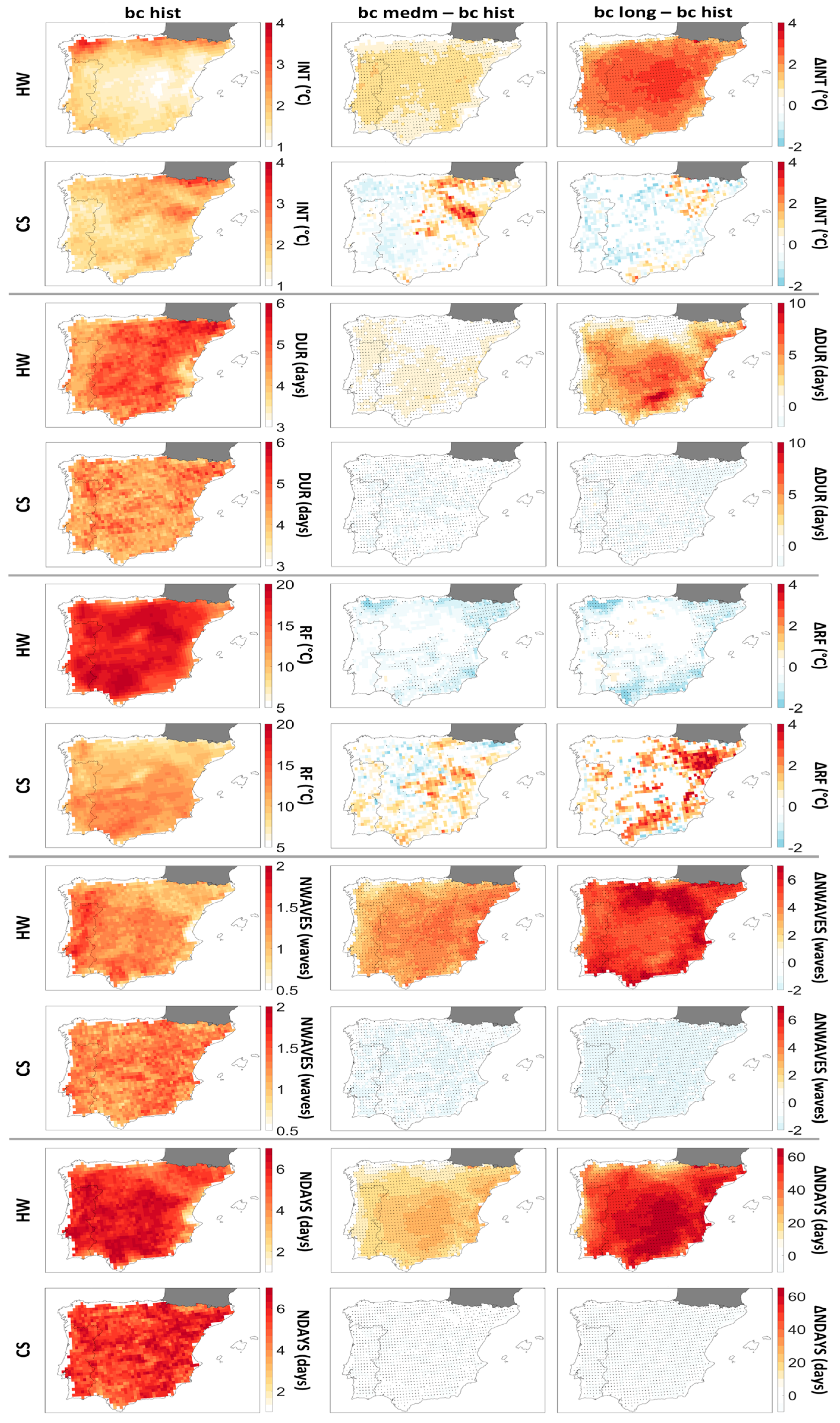
3.2.3. Heat Waves and Cold Spells

As mentioned above, heat waves and cold spells are characterized by their intensity (INT), duration (DUR), recovery factor (RF), waves’/spells’ number (NWAVES), and number of wave/spell days (NDAYS). These events were defined for summer (June to August) and for winter (December to February), respectively.
Figure 10 shows the mean spatial distribution of these properties for heat waves and cold spells in the historical period, the differences between the medium- and long-term future and the historical period, and the respective statistical significance. In the future, heat waves are projected to have a statistically significant increase in their intensity, duration, waves’ number, and number of wave days. This increase is more pronounced in the long-term future, in which we verify a mean maximum increase of the intensity and duration of 4 °C and 10 days, respectively, resulting in the doubling of the maximum intensity and in the triple of the duration of the historical period. During the long-term future, a mean maximum increase greater than 6 waves and 60 wave days (around 2 months, that is, 2/3 of summer), which corresponds to threefold and 10-fold the wave’s number and number of wave days observed during the historical period, respectively, is expected. A significant decrease in the recovery factor in some small areas is also expected, whereas in others there are no significant differences.
The results show a future increase in the waves’ number, their duration, and intensity. Other studies [6,20,70,71,81,82,83] found the same results for number, duration, and intensity of heat waves.
Cold spells are estimated to have a predominant significant decrease in their duration, spells’ number, and number of spell days, associated with the increase in the minimum temperature. The intensity and the recovery factor have a variable behavior in the future. Thus, there are verified non-significant positive and negative differences, according to the region and period of study, although both future periods are majorly characterized by a decrease in the intensity. The recovery factor is defined by regions with an increase and decrease during the medium-term future, while in the long-term future, its predominant increase is verified. In the medium-term future, certain areas have no cold spells, which is more considerable in the long-term future.
Few studies focused on cold spells, although some studies presented a future decrease of the cold spells’ number, their duration, and intensity [20,84].
Because cold spells are expected to be less frequent in the future and heat waves are expected to increase, one expects these to represent several environmental and socio-economic negative impacts [3,21,83,85], influencing, for example, the ecosystems, human society and mortality, and regional economies. To further illustrate this, we focused on the heat waves with the longest duration that occurred in Madrid during the historical and future periods (Figure 11). The selection of this characteristic (i.e., duration) is based on evidence that suggests that, concerning impacts, the duration of the heat waves might be more important than the intensity [86].
In the future periods, an increase of the duration and intensity of the heat waves is verified, while the recovery factor remains unchanged. These results are similar to those previously presented in Figure 10. During the historical period, the longest heat wave was characterized by a duration of 11 days and an intensity of around 1 °C. In the long-term future, the duration increased to 76 days, which corresponds to a consecutive period of longer than 2 months, and the intensity increased five times (5.79 °C). We observe that this mega heat wave has temperatures exceeding 40 °C most days and some consecutive days of more than 45 °C.

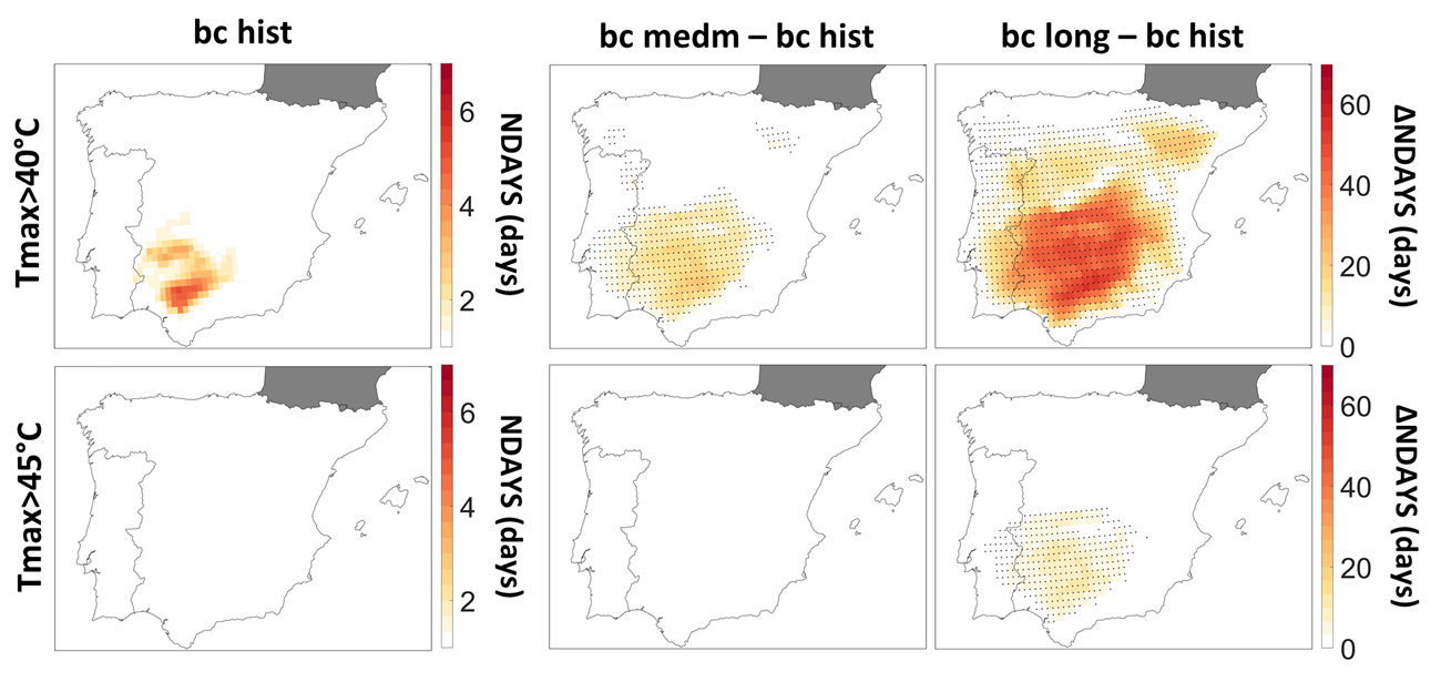
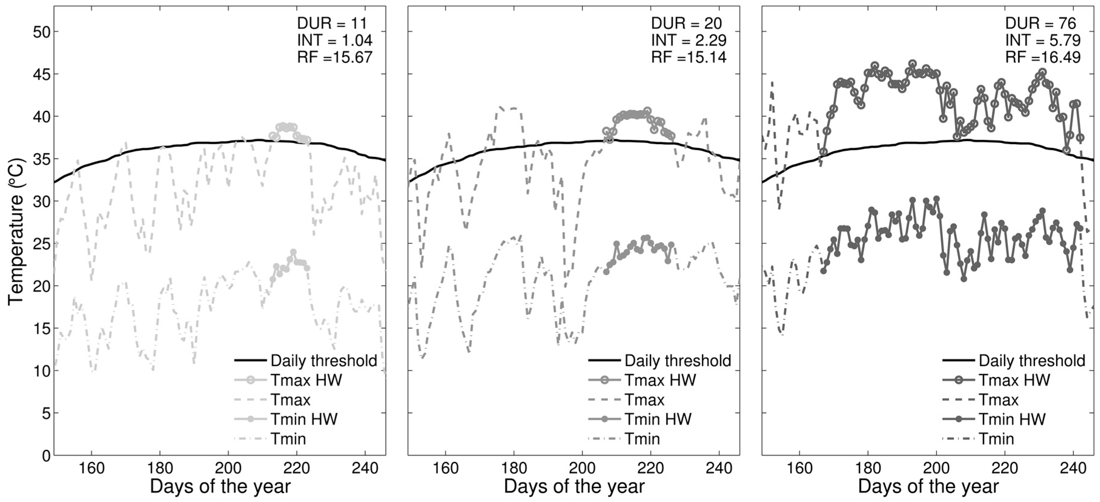
3.2.4. Extreme Heat Waves

To obtain more insight into very extreme high temperature heat wave events, we combined the heat wave definition with high maximum temperature thresholds, namely 25 °C, 35 °C, 40 °C, and 45 °C. Thus, the daily threshold used to identify heat waves was a combination of the exceedance of a fixed absolute value and the usual deviation from the heat wave threshold derived in Section 2.2.3.
Figure 12 shows the mean spatial distribution of the number of heat wave days for the historical climate and the differences between the future and historical periods. This was done for heat waves using thresholds of maximum temperature equal to 25, 35, 40, and 45 °C. In the future, a statistically significant increase in the number of heat wave days is expected, when compared with the historical period. This increase is more pronounced for the lower thresholds (25 and 35 °C) with significant differences higher than 60 days in the long-term future for heat waves with temperatures over 25 °C. For the heat waves with maximum temperature higher than 35 °C, such differences were not observed in the northern regions. For the medium-term future, the coastal northern region was characterized by the inexistence of heat waves with maximum temperatures higher than 35 °C, contrary to what happens in the long-term future.
Regarding the higher threshold temperatures (40 and 45 °C), the historical period is characterized by the almost inexistence of such extreme heat waves. In the medium-term future, the number of heat wave days with maximum temperatures higher than 40 °C increases significantly in the central/southern region, which includes cities such as Évora and Seville, while for the long-term future the area significantly increases, covering most of the Iberian Peninsula. The largest differences are observed in regions that already had heat wave days with maximum temperatures surpassing 40 °C in the medium-term future, reaching values higher than 40 days. Concerning the most extreme heat waves, with maximum temperatures higher than 45 °C, the historic and medium-term future have few such heat wave days, whereas, for the long-term future, one may expect around an annual average of up to 20 heat wave days with maximum temperatures higher than 45 °C, with these occurring in the central/southern non-coastal region. We note, however, that the total annual average number of up to two consecutive days (i.e., not heat waves) with maximum temperatures above these thresholds are slightly higher than those shown in Figure 12.

4. Conclusions

The main purpose of this study was to assess extreme temperature climate changes over the Iberian Peninsula. For that, different methods and various aspects of extreme temperatures, such as heat waves and cold spells, were analyzed. A set of climate simulations performed by the WRF regional climate model and forced by the MPI-ESM-LR global climate model for the Iberian Peninsula were used. The evaluation of the future change in extreme temperatures was accomplished through the differences of two future climate scenarios—medium-term (2046–2065) and long-term (2081–2100)—relative to a historical reference climate (1986–2005), considering the future greenhouse gas emission scenario RCP8.5. The statistical significance of these changes was also assessed.
Simulated daily maximum temperature was underestimated to different degrees along the distribution, relative to the observations, while simulated minimum temperature was predominantly underestimated during summer and overestimated during winter. These systematic errors were minimized after the application of bias correction in the form of quantile mapping to simulated daily maximum and minimum temperature using observationally derived temperature data (E-OBS).
The change in extreme temperature and its statistical significance was evaluated through the differences between the future climates and the historical climate.
In the medium- and long-term future, a statistically significant increase in both minimum and maximum temperatures greater than 2 °C and 4 °C, respectively, is expected but more pronounced during summer with warming in excess of 6 °C in some regions. This is in line with an increase in the annual number of summer days and tropical nights and a decrease of the annual number of frost days.
For heat waves and for both future climates, an increase in their intensity, duration, and waves’ number is estimated. The number of heat wave days is estimated to increase from an annual average of 6 in the historical climate to 20 and 50 over much of the region for the medium- and long-term climate, respectively. A small decrease in the recovery factor is observed. On the contrary, for cold spells, a decrease in the intensity, duration, spells’ number, and number of spell days and an increase in the recovery factor are expected. These differences are more pronounced for the heat waves and are statistically significant in most cases for most of the Iberian Peninsula.
These results are in line with the existing literature applying bias correction before assessing extreme events. Recent studies show that heat waves become more frequent and have higher mean duration and intensity. Moreover, heat waves can occur during a larger part of summer [87]. Other studies show the same future warming with an increase for severe heat waves [88].
Finally, we analyzed the most extreme heat waves as being those in which each day has maximum temperatures above 25 °C, 35 °C, 40 °C, and 45 °C. In the future, a significant increase in heat wave days with extreme maximum temperatures is expected. For the long-term future, the central/southern region of the Iberian Peninsula may experience an average of between 10 and 20 heat wave days per year with maximum temperatures surpassing 45 °C in each wave day. For some locations in the southern/central non-costal region we identified heat waves that may last nearly the whole summer, with average maximum temperatures of about 40 °C. These type of mega heat waves were not found in the historic and medium-term future climates.
These results should be considered in the development of extreme temperature-related adaptation measures in various socio-economic areas.

Author Contributions

Conceptualization, A.R.; methodology, C.V., S.C.P., and A.R.; investigation, C.V., S.C.P, and A.R.; original draft preparation, C.V.; review and editing, S.C.P. and A.R.; and supervision, A.R.

Funding

This work is supported by the Fundação para a Ciência e Tecnologia (FCT) (Portugal) through the PhD grant reference SFRH/BD/129154/2017. The authors also wish to thank the financial support of FEDER through the COMPETE Programme and the national funds from FCT—Science and Technology Portuguese Foundation for financing the DOUROZONE project (PTDC/AAG-MAA/3335/2014; POCI-01-0145-FEDER-016778). The authors wish to thank the Department of Physics (University of Aveiro). Thanks are also due for the financial support to CESAM (UID/AMB/50017/2019) to FCT/MEC through national funds and the co-funding by the FEDER within the PT2020 Partnership Agreement and Compete 2020.

Acknowledgments

The author wish to acknowledge the E-OBS dataset from the EU-FP6 project ENSEMBLES (http://ensembles-eu.metoffice.com) and the data providers in the ECA&D project (http://www.ecad.eu).

Conflicts of Interest

The authors declare no conflict of interest.

References

  1. Marengo, J.A.; Rusticucci, M.; Penalba, O.; Renom, M. An intercomparison of observed and simulated extreme rainfall and temperature events during the last half of the twentieth century: Part 2: Historical trends. Clim. Chang. 2010, 98, 509–529. [Google Scholar] [CrossRef]
  2. Meehl, G.A.; Karl, T.; Easterling, D.R.; Changnon, S.; Pielke, R., Jr.; Changnon, D.; Evans, J.; Groisman, P.Y.; Knutson, T.R.; Kunkel, K.E.; et al. An Introduction to Trends in Extreme Weather and Climate Events: Observations, Socioeconomic Impacts, Terrestrial Ecological Impacts, and Model Projections. Bull. Am. Meteorol. Soc. 2000, 81, 413–416. [Google Scholar] [CrossRef]
  3. Easterling, D.R.; Meehl, G.A.; Parmesan, C.; Changnon, S.A.; Karl, T.R.; Mearns, L.O. Climate Extremes: Observations, Modeling, and Impacts. Science 2000, 289, 2068–2074. [Google Scholar] [CrossRef] [Green Version]
  4. Mora, C.; Dousset, B.; Caldwell, I.R.; Powell, F.E.; Geronimo, R.C.; Bielecki, C.R.; Counsell, C.W.W.; Dietrich, B.S.; Johnston, E.T.; Louis, L.V.; et al. Global risk of deadly heat. Nat. Clim. Chang. 2017, 7, 501–506. [Google Scholar] [CrossRef]
  5. Sánchez, E.; Gallardo, C.; Gaertner, M.A.; Arribas, A.; Castro, M. Future climate extreme events in the Mediterranean simulated by a regional climate model: A first approach. Glob. Planet. Chang. 2004, 44, 163–180. [Google Scholar] [CrossRef]
  6. Beniston, M.; Stephenson, D.B.; Christensen, O.B.; Ferro, C.A.T.; Frei, C.; Goyette, S.; Halsnaes, K.; Holt, T.; Jylhä, K.; Koffi, B.; et al. Future extreme events in European climate: An exploration of regional climate model projections. Clim. Chang. 2007, 81, 71–95. [Google Scholar] [CrossRef]
  7. Suklitsch, M.; Gobiet, A.; Truhetz, H.; Awan, N.K.; Göttel, H.; Jacob, D. Error characteristics of high resolution regional climate models over the Alpine area. Clim. Dyn. 2011, 37, 377–390. [Google Scholar] [CrossRef]
  8. Teutschbein, C.; Seibert, J. Bias correction of regional climate model simulations for hydrological climate-change impact studies: Review and evaluation of different methods. J. Hydrol. 2012, 456–457, 12–29. [Google Scholar] [CrossRef]
  9. Hnilica, J.; Hanel, M.; Puš, V. Multisite bias correction of precipitation data from regional climate models. Int. J. Clim. 2017, 37, 2934–2946. [Google Scholar] [CrossRef]
  10. Moberg, A.; Jones, P.D. Regional climate model simulations of daily maximum and minimum near-surface temperatures across Europe compared with observed station data 1961–1990. Clim. Dyn. 2004, 23, 695–715. [Google Scholar] [CrossRef]
  11. Déqué, M. Frequency of precipitation and temperature extremes over France in an anthropogenic scenario: Model results and statistical correction according to observed values. Glob. Planet. Chang. 2007, 57, 16–26. [Google Scholar] [CrossRef]
  12. Amengual, A.; Homar, V.; Romero, R.; Alonso, S.; Ramis, C. A statistical Adjustment of Regional Climate Model Outputs to Local Scales: Application to Platja de Palma, Spain. J. Clim. 2012, 25, 939–957. [Google Scholar] [CrossRef]
  13. Ngai, S.T.; Tangang, F.; Juneng, L. Bias correction of global and regional simulated daily precipitation and surface mean temperature over Southeast Asia using quantile mapping method. Glob. Planet. Chang. 2017, 149, 79–90. [Google Scholar] [CrossRef]
  14. Fonseca, D.; Carvalho, M.J.; Marta-Almeida, M.; Melo-Gonçalves, P.; Rocha, A. Recent trends of extreme temperature indices for the Iberian Peninsula. Phys. Chem. Earth 2016, 94, 66–76. [Google Scholar] [CrossRef]
  15. Alexander, L.V.; Zhang, X.; Peterson, T.C.; Caesar, J.; Gleason, B.; Klein Tank, A.M.G.; Haylock, M.; Collins, D.; Trewin, B.; Rahimzadeh, F.; et al. Global observed changes in daily climate extremes of temperature and precipitation. J. Geophys. Res. 2006, 111, D05109. [Google Scholar] [CrossRef]
  16. Goubanova, K.; Li, L. Extremes in temperature and precipitation around the Mediterranean basin in an ensemble of future climate scenario simulations. Glob. Planet. Chang. 2007, 57, 27–42. [Google Scholar] [CrossRef]
  17. Giorgi, F.; Lionello, P. Climate change projections for the Mediterranean region. Glob. Planet. Chang. 2008, 63, 90–104. [Google Scholar] [CrossRef]
  18. Sillmann, J.; Roeckner, E. Indices for extreme events in projections of anthropogenic climate change. Clim. Chang. 2008, 86, 83–104. [Google Scholar] [CrossRef]
  19. Sillmann, J.; Kharin, V.V.; Zwiers, F.W.; Zhang, X.; Bronaugh, D. Climate extremes indices in the CMIP5 multimodel ensemble: Part 2. Future climate projections. J. Geophys. Res. Atmos. 2013, 118, 2473–2493. [Google Scholar] [CrossRef] [Green Version]
  20. Pereira, S.C.; Marta-Almeida, M.; Carvalho, A.C.; Rocha, A. Heat wave and cold spell changes in Iberia for a future climate scenario. Int. J. Clim. 2017, 37, 5192–5205. [Google Scholar] [CrossRef]
  21. Zuo, J.; Pullen, S.; Palmer, J.; Bennetts, H.; Chileshe, N.; Ma, T. Impacts of heat waves and corresponding measures: A review. J. Clean. Prod. 2015, 92, 1–12. [Google Scholar] [CrossRef]
  22. Marta-Almeida, M.; Teixeira, J.C.; Carvalho, M.J.; Melo-Gonçalves, P.; Rocha, A.M. High resolution WRF climatic simulations for the Iberian Peninsula: Model validation. Phys. Chem. Earth 2016, 94, 94–105. [Google Scholar] [CrossRef]
  23. Skamarock, W.C.; Klemp, J.B.; Dudhia, J.; Gill, D.O.; Barker, D.M.; Duda, M.G.; Huang, X.-Y.; Wang, W.; Powers, J.G. A Description of the Advanced Research WRF Version 3; National Center for Atmospheric Research: Boulder, CO, USA, 2008. [Google Scholar] [CrossRef]
  24. Pradhan, P.K.; Liberato, M.L.R.; Ferreira, J.A.; Dasamsetti, S.; Vijaya Bhaskara Rao, S. Characteristics of different convective parameterization schemes on the simulation of intensity and track of severe extratropical cyclones over North Atlantic. Atmos. Res. 2018, 199, 128–144. [Google Scholar] [CrossRef]
  25. Efstathiou, G.A.; Zoumakis, N.M.; Melas, D.; Lolis, C.J.; Kassomenos, P. Sensitivity of WRF to boundary layer parameterizations in simulating a heavy rainfall event using different microphysical schemes. Effect on large-scale processes. Atmos. Res. 2013, 132–133, 125–143. [Google Scholar] [CrossRef]
  26. Sharma, A.; Fernando, H.J.S.; Hamlet, A.F.; Hellmann, J.J.; Barlage, M.; Chen, F. Urban meteorological modeling using WRF: A sensitivity study. Int. J. Clim. 2017, 37, 1885–1900. [Google Scholar] [CrossRef]
  27. Katragkou, E.; Garciá-Diéz, M.; Vautard, R.; Sobolowski, S.; Zanis, P.; Alexandri, G.; Cardoso, R.M.; Colette, A.; Fernandez, J.; Gobiet, A.; et al. Regional climate hindcast simulations within EURO-CORDEX: Evaluation of a WRF multi-physics ensemble. Geosci. Model Dev. 2015, 8, 603–618. [Google Scholar] [CrossRef]
  28. Cardoso, R.M.; Soares, P.M.M.; Miranda, P.M.A.; Belo-Pereira, M. WRF high resolution simulation of Iberian mean and extreme precipitation climate. Int. J. Clim. 2013, 33, 2591–2608. [Google Scholar] [CrossRef]
  29. Fita, L.; Fernández, J.; García-Díez, M. CLWRF: WRF modifications for regional climate simulation under future scenarios. In Preprints, 11th WRF Users’ Event; NCAR: Boulder, CO, USA, 2010; p. 26. [Google Scholar] [CrossRef]
  30. Giorgetta, M.A.; Jungclaus, J.; Reick, C.H.; Legutke, S.; Bader, J.; Böttinger, M.; Brovkin, V.; Crueger, T.; Esch, M.; Fieg, K.; et al. Climate and carbon cycle changes from 1850 to 2100 in MPI-ESM simulations for the Coupled Model Intercomparison Project phase 5. J. Adv. Model. Earth Syst. 2013, 5, 572–597. [Google Scholar] [CrossRef] [Green Version]
  31. Ferreira, A.P.G.F. Sensibilidade às Parametrizações físicas do WRF nas Previsões à Superfície em Portugal Continental, Internship Report in Meteorology and Physical Oceanography, University of Aveiro. 2007. Available online: http://climetua.fis.ua.pt/publicacoes/Estagio_PauloFerreira.pdf (accessed on 19 April 2019).
  32. Hong, S.-Y.; Lim, J.-O.J. The WRF Single-Moment 6-Class Microphysics Scheme (WSM6). J. Korean Meteorol. Soc. 2006, 42, 129–151. [Google Scholar]
  33. Dudhia, J. Numerical Study of Convection Observed during the Winter Monsoon Experiment Using a Mesoscale Two-Dimensional Model. J. Atmos. Sci. 1989, 46, 3077–3107. [Google Scholar] [CrossRef] [Green Version]
  34. Mlawer, E.J.; Clough, S.A. On the Extension of Rapid Radiative Transfer Model to the Shortwave Region. In Proceedings of the 6th Atmospheric Radiation Measurement (ARM) Science Team Meeting, US Department of Energy, Washington, DC, USA, 4–7 March 1996; CONF-9603149. pp. 223–226. [Google Scholar]
  35. Zhang, D.; Anthes, R.A. A High-Resolution Model of the Planetary Boundary Layer-Sensivity Tests and Comparisons with SESAME-79 Data. J. Appl. Meteorol. 1982, 21, 1594–1609. [Google Scholar] [CrossRef]
  36. Tewari, M.; Chen, F.; Wang, W.; Dudhia, J.; LeMone, M.A.; Mitchell, K.; Ek, M.; Gayno, G.; Wegiel, J.; Cuenca, R.H. Implementation and verification of the unified NOAH land surface model in the WRF model. In Proceedings of the 20th Conference on Weather Analysis and Forecasting/16th Conference on Numerical Weather Prediction, Seatle, WA, USA, 12–16 January 2004. [Google Scholar]
  37. Grell, G.A.; Freitas, S.R. A scale and aerosol aware stochastic convective parameterization for weather and air quality modeling. Atmos. Chem. Phys. 2014, 14, 5233–5250. [Google Scholar] [CrossRef] [Green Version]
  38. Bossard, M.; Feranec, J.; Otahel, J. CORINE Land Cover Technical Guide-Addendum 2000; European Environment Agency Technical Report 40; European Environment Agency: Copenhagen, Denmark, 2000.
  39. Pineda, N.; Jorba, O.; Jorge, J.; Baldasano, J.M. Using NOAA AVHRR and SPOT VGT data to estimate surface parameters: Application to a mesoscale meteorological model. Int. J. Remote Sens. 2004, 25, 129–143. [Google Scholar] [CrossRef]
  40. Teixeira, J.C.; Carvalho, A.C.; Carvalho, M.J.; Luna, T.; Rocha, A. Sensitivity of the WRF model to the lower boundary in an extreme precipitation event-Madeira island case study. Nat. Hazards Earth Syst. Sci. 2014, 14, 2009–2025. [Google Scholar] [CrossRef]
  41. Miguez-Macho, G.; Stenchikov, G.L.; Robock, A. Spectral nudging to eliminate the effects of domain position and geometry in regional climate model simulations. J. Geophys. Res. 2004, 109, D13104. [Google Scholar] [CrossRef]
  42. Taylor, K.E.; Stouffer, R.J.; Meehl, G.A. An overview of CMIP5 and the experiment design. Bull. Am. Meteorol. Soc. 2012, 93, 485–498. [Google Scholar] [CrossRef]
  43. IPCC. Climate Change 2014; Synthesis Report. Contribution of Working Groups I, II and III to the Fifth Assessment Report of the Intergovernmental Panel on Climate Change; IPCC: Geneva, Switzerland, 2014; p. 151. [Google Scholar] [CrossRef]
  44. Moss, R.; Babiker, M.; Brinkman, S.; Calvo, E.; Carter, T.; Edmonds, J.; Elgizouli, I.; Emori, S.; Erda, L.; Hibbard, K.; et al. Towards New Scenarios for Analysis of Emissions, Climate Change, Impacts and Response Strategies; Technical Summary; Intergovernmental Panel on Climate Change (IPCC): Geneva, Switzerland, 2008; p. 25. [Google Scholar]
  45. Viceto, C.; Marta-Almeida, M.; Rocha, A. Future climate change of stability indices for the Iberian Peninsula. Int. J. Clim. 2017, 37, 4390–4408. [Google Scholar] [CrossRef]
  46. Bartolomeu, S.; Carvalho, M.J.; Marta-Almeida, M.; Melo-Gonçalves, P.; Rocha, A. Recent trends of extreme precipitation indices in the Iberian Peninsula using observations and WRF model results. Phys. Chem. Earth 2016, 94, 10–21. [Google Scholar] [CrossRef]
  47. Carvalho, M.J.; Melo-Gonçalves, P.; Teixeira, J.C.; Rocha, A. Regionalization of Europe based on a K -Means Cluster Analysis of the climate change of temperatures and precipitation. Phys. Chem. Earth 2016, 94, 22–28. [Google Scholar] [CrossRef]
  48. Haylock, M.R.; Hofstra, N.; Klein Tank, A.M.G.; Klok, E.J.; Jones, P.D.; New, M. A European daily high-resolution gridded data set of surface temperature and precipitation for 1950-2006. J. Geophys. Res. Atmos. 2008, 113, D20119. [Google Scholar] [CrossRef]
  49. Hofstra, N.; Haylock, M.; New, M.; Jones, P.D. Testing E-OBS European high-resolution gridded data set of daily precipitation and surface temperature. J. Geophys. Res. 2009, 114, D21101. [Google Scholar] [CrossRef]
  50. Kostopoulou, E.; Giannakopoulos, C.; Hatzaki, M.; Tziotziou, K. Climate extremes in the NE Mediterranean: Assessing the E-OBS dataset and regional climate simulations. Clim. Res. 2012, 54, 249–270. [Google Scholar] [CrossRef]
  51. Student. The Probable Error of a Mean. Biometrika 1908, 6, 1–25. [Google Scholar] [CrossRef]
  52. Wilks, D.S. Statistical Methods in the Atmospheric Sciences. Int. Geophys. Ser. 2006, 91, 649. [Google Scholar] [CrossRef]
  53. Dosio, A.; Paruolo, P.; Rojas, R. Bias correction of the ENSEMBLES high resolution climate change projections for use by impact models: Analysis of the climate change signal. J. Geophys. Res. Atmos. 2012, 117, D17110. [Google Scholar] [CrossRef]
  54. Dosio, A. Projections of climate change indices of temperature and precipitation from an ensemble of bias-adjusted high-resolution EURO-CORDEX regional climate models. J. Geophys. Res. Atmos. 2016, 121, 5488–5511. [Google Scholar] [CrossRef] [Green Version]
  55. Sippel, S.; Otto, F.E.L.; Forkel, M.; Allen, M.R.; Guillod, B.P.; Heimann, M.; Reichstein, M.; Seneviratne, S.I.; Thonicke, K.; Mahecha, M.D. A novel bias correction methodology for climate impact simulations. Earth Syst. Dyn. 2016, 7, 71–88. [Google Scholar] [CrossRef]
  56. Piani, C.; Haerter, J.O.; Coppola, E. Statistical bias correction for daily precipitation in regional climate models over Europe. Appl. Clim. 2010, 99, 187–192. [Google Scholar] [CrossRef]
  57. Piani, C.; Weedon, G.P.; Best, M.; Gomes, S.M.; Viterbo, P.; Hagemann, S.; Haerter, J.O. Statistical bias correction of global simulated daily precipitation and temperature for the application of hydrological models. J. Hydrol. 2010, 395, 199–215. [Google Scholar] [CrossRef]
  58. Themeßl, M.J.; Gobiet, A.; Heinrich, G. Empirical-statistical downscaling and error correction of regional climate models and its impact on the climate change signal. Clim. Chang. 2012, 112, 449–468. [Google Scholar] [CrossRef]
  59. Maraun, D. Bias Correction, Quantile Mapping, and Downscaling: Revisiting the Inflation Issue. J. Clim. 2013, 26, 2137–2143. [Google Scholar] [CrossRef] [Green Version]
  60. Casanueva, A.; Kotlarski, S.; Herrera, S.; Fernández, J.; Gutiérrez, J.M.; Boberg, F.; Colette, A.; Christensen, O.B.; Goergen, K.; Jacob, D.; et al. Daily precipitation statistics in a EURO-CORDEX RCM ensemble: Added value of raw and bias-corrected high-resolution simulations. Clim. Dyn. 2016, 47, 719–737. [Google Scholar] [CrossRef]
  61. Casanueva, A.; Bedia, J.; Herrera, S.; Fernández, J.; Gutiérrez, J.M. Direct and component-wise bias correction of multi-variate climate indices: The percentile adjustment function diagnostic tool. Clim. Chang. 2018, 147, 411–425. [Google Scholar] [CrossRef]
  62. Maraun, D.; Shepherd, T.G.; Widmann, M.; Zappa, G.; Walton, D.; Gutiérrez, J.M.; Hagemann, S.; Richter, I.; Soares, P.M.M.; Hall, A.; Mearns, L.O. Towards process-informed bias correction of climate change simulations. Nat. Clim. Chang. 2017, 7, 764–773. [Google Scholar] [CrossRef]
  63. Hertig, E.; Maraun, D.; Bartholy, J.; Pongracz, R.; Vrac, M.; Mares, I.; Gutiérrez, J.M.; Wibig, J.; Casanueva, A.; Soares, P.M.M. Comparison of statistical downscaling methods with respect to extreme events over Europe: Validation results from the perfect predictor experiment of the COST Action VALUE. Int. J. Clim. 2018, 1–22. [Google Scholar] [CrossRef]
  64. Ivanov, M.A.; Luterbacher, J.; Kotlarski, S. Climate model biases and modification of the climate change signal by intensity-dependent bias correction. J. Clim. 2018, 31, 6591–6610. [Google Scholar] [CrossRef]
  65. Li, H.; Sheffield, J.; Wood, E.F. Bias correction of monthly precipitation and temperature fields from Intergovernmental Panel on Climate Change AR4 models using equidistant quantile matching. J. Geophys. Res. Atmos. 2010, 115, D10101. [Google Scholar] [CrossRef]
  66. Wilcke, R.A.I.; Mendlik, T.; Gobiet, A. Multi-variable error correction of regional climate models. Clim. Chang. 2013, 120, 871–887. [Google Scholar] [CrossRef] [Green Version]
  67. Maraun, D.; Widmann, M. Cross-validation of bias-corrected climate simulations is misleading. Hydrol. Earth Syst. Sci. 2018, 22, 4867–4873. [Google Scholar] [CrossRef]
  68. Zhang, X.; Alexander, L.; Hegerl, G.C.; Jones, P.; Tank, A.K.; Peterson, T.C.; Trewin, B.; Zwiers, F.W. Indices for monitoring changes in extremes based on daily temperature and precipitation data. Wires Clim. Chang. 2011, 2, 851–870. [Google Scholar] [CrossRef]
  69. Climdex. 2019. Available online: https://www.climdex.org/learn/indices/ (accessed on 19 March 2019).
  70. Tebaldi, C.; Hayhoe, K.; Arblaster, J.M.; Meehl, G.A. Going to the extremes: An intercomparison of model-simulated historical and future changes in extreme events. Clim. Chang. 2006, 79, 185–211. [Google Scholar] [CrossRef]
  71. Russo, S.; Dosio, A.; Graversen, R.G.; Sillmann, J.; Carrao, H.; Dunbar, M.B.; Singleton, A.; Montagna, P.; Barbola, P.; Vogt, J.V. Magnitude of extreme heat waves in present climate and their projection in a warming world. J. Geophys. Res. Atmos. 2014, 119, 12500–12512. [Google Scholar] [CrossRef]
  72. Morabito, M.; Crisci, A.; Messeri, A.; Messeri, G.; Betti, G.; Orlandini, S.; Raschi, A.; Maracchi, G. Increasing Heatwave Hazards in the Southeastern European Union Capitals. Atmosphere 2017, 8, 115. [Google Scholar] [CrossRef]
  73. Acero, F.J.; Fernández-Fernández, M.I.; Carrasco, V.M.S.; Parey, S.; Hoang, T.T.H.; Dacunha-Castelle, D.; García, J.A. Changes in heat wave characteristics over Extremadura (SW Spain). Appl. Clim. 2018, 133, 605–617. [Google Scholar] [CrossRef]
  74. Robinson, P.J. On the Definition of a Heat Wave. J. Appl. Meteorol. 2001, 40, 762–775. [Google Scholar] [CrossRef]
  75. Russo, S.; Sillmann, J.; Sterl, A. Humid heat waves at different warming levels. Sci. Rep. 2017, 7, 7477. [Google Scholar] [CrossRef] [PubMed] [Green Version]
  76. Hansen, J.; Sato, M.; Ruedy, R. Perception of climate change. Proc. Natl. Acad. Sci. USA 2012, 109, E2415–E2423. [Google Scholar] [CrossRef] [Green Version]
  77. Ramos, A.M.; Trigo, R.M.; Santo, F.E. Evolution of extreme temperatures over Portugal: Recent changes and future scenarios. Clim. Res. 2011, 48, 177–192. [Google Scholar] [CrossRef]
  78. Cattiaux, J.; Douville, H.; Peings, Y. European temperatures in CMIP5: Origins of present-day biases and future uncertainties. Clim. Dyn. 2013, 41, 2889–2907. [Google Scholar] [CrossRef]
  79. Donat, M.G.; Alexander, L.V.; Yang, H.; Durre, I.; Vose, R.; Dunn, R.J.H.; Willett, K.M.; Aguilar, E.; Brunet, M.; Caesar, J.; et al. Updated analyses of temperature and precipitation extreme indices since the beginning of the twentieth century: The HadEX2 dataset. J. Geophys. Res. Atmos. 2013, 118, 2098–2118. [Google Scholar] [CrossRef] [Green Version]
  80. Tank, A.M.G.K.; Können, G.P. Trends in Indices of Daily Temperature and Precipitation Extremes in Europe, 1946–99. J. Clim. 2003, 16, 3665–3680. [Google Scholar] [CrossRef] [Green Version]
  81. Schoetter, R.; Cattiaux, J.; Douville, H. Changes of western European heat wave characteristics projected by the CMIP5 ensemble. Clim. Dyn. 2015, 45, 1601–1616. [Google Scholar] [CrossRef]
  82. Bador, M.; Terray, L.; Boé, J.; Somot, S.; Alias, A.; Gibelin, A.-L.; Dubuisson, B. Future summer mega-heatwave and record-breaking temperatures in a warmer France climate. Environ. Res. Lett. 2017, 12, 074025. [Google Scholar] [CrossRef] [Green Version]
  83. Meehl, G.A.; Tebaldi, C. More intense, More Frequent, and Longer Lasting Heat Waves in the 21st Century. Science 2004, 305, 994–997. [Google Scholar] [CrossRef] [PubMed]
  84. Peterson, T.C.; Heim, R.R., Jr.; Hirsch, R.; Kaiser, D.P.; Brooks, H.; Diffenbaugh, N.S.; Dole, R.M.; Giovannettone, J.P.; Guirguis, K.; Karl, T.R.; et al. Monitoring and Understanding Changes in Heat Waves, Cold Waves, Floods, and Droughts in the United States: State of Knowledge. Bull. Am. Meteorol. Soc. 2013, 94, 821–834. [Google Scholar] [CrossRef]
  85. Gasparrini, A.; Armstrong, B. The impact of heat waves on mortality. Epidemiology 2012, 22, 68–73. [Google Scholar] [CrossRef]
  86. D’Ippoliti, D.; Michelozzi, P.; Marino, C.; de’Donato, F.; Menne, B.; Katsouyanni, K.; Kirchmayer, U.; Analitis, A.; Medina-Ramón, M.; Paldy, A.; et al. The impact of heat waves on mortality in 9 European cities: Results from the EuroHEAT project. Environ. Heal. 2010, 9, 37. [Google Scholar] [CrossRef]
  87. Ouzeau, G.; Soubeyroux, J.-M.; Schneider, M.; Vautard, R.; Planton, S. Heat waves analysis over France in present and future climate: Application of a new method on the EURO-CORDEX ensemble. Clim. Serv. 2016, 4, 1–12. [Google Scholar] [CrossRef] [Green Version]
  88. Lhotka, O.; Kyselý, J.; Plavcová, E. Evaluation of major heat waves’ mechanisms in EURO-CORDEX RCMs over Central Europe. Clim. Dyn. 2018, 50, 4249–4262. [Google Scholar] [CrossRef]
Figure 1. (a) Configuration of the domains used in the regional Weather Research and Forecasting (WRF) model implementation. The model ran in two-way nesting mode with increasing domain resolutions of 81 km (D-1), 27 km (D-2), and 9 km (D-3); (b) topography of the study area (Iberian Peninsula); WRF domain D-3 (9 km resolution) and domain D-3* (0.2° resolution). In this study, we used domain D-3*.
Atmosphere 10 00229 g001
Figure 2. Graphical scheme of the bias correction (bc) of maximum temperature (Tmax, °C) for Madrid for only the long-term future. Cumulative distribution function (CDF) of the observations, simulations with no bias correction of the historical and long-term future periods (no bc hist and no bc long, respectively), and bias correction of the long-term future period (bc long). Vertical lines show the mean values of historical and long-term future simulations before bias correction.
Atmosphere 10 00229 g002
Figure 3. Mean daily maximum and minimum temperature (Tmax and Tmin, °C) [first row, annual; second row, winter (DJF); third row, summer (JJA)] of the observations (obs) and the simulations with no and with bias correction (no bc hist and bc hist, respectively) for the historical period. Differences between the mean spatial distribution with no and with bias correction and the observations (no bc hist–obs and bc hist–obs, respectively). Statistically significant differences (Student’s t-test) at 5% significance level are represented by black dots.
Atmosphere 10 00229 g003
Figure 4. Quantile–quantile plot of observations (x-axis) vs. no bias correction of the historical period (no bc hist, y-axis) for the daily maximum (left) and minimum temperature (°C) (right) for Madrid. Black solid line represents similar x-axis and y-axis quantiles.
Atmosphere 10 00229 g004
Figure 5. Cumulative distribution function (first row) and probability density function (PDF, second row) of the simulations with no bias correction of the historical period (no bc hist), observations and bias correction of the historical period (bc hist) for the daily maximum and minimum temperature (Tmax and Tmin, °C) (first and second column, respectively) for Madrid.
Atmosphere 10 00229 g005
Figure 6. Mean daily maximum and minimum temperature (Tmax and Tmin, °C) for the historical period (bc hist, first column). Differences between the medium- and long-term future and the historical period [bc medm–bc hist (second column) and bc long–bc hist (third column), respectively]. Statistically significant differences (Student’s t-test) at 5% significance level were verified in all the grid points.
Atmosphere 10 00229 g006
Figure 7. Quantile–quantile plot of the historical period (bc hist, x-axis) vs. the medium-term future (bc medm, medium grey, left y-axis) and the long-term future (bc long, dark grey, right y-axis), for daily maximum and minimum temperature (Tmax and Tmin, °C) (left and right, respectively) for Madrid. Black solid line represents similar x-axis and y-axis quantiles.
Atmosphere 10 00229 g007
Figure 8. Cumulative distribution function (CDF) of the historical period (bc hist), medium- (bc medm), and long-term future (bc long), for the daily maximum and minimum temperature (Tmax and Tmin, °C) (left and right, respectively) for Madrid.
Atmosphere 10 00229 g008
Figure 9. Climate change indices—mean number of summer days (SU25, days per year, first row), mean number of frost days (FD0, days per year, second row), and mean number of tropical nights (TR20, nights per year, third row)—for the historical period (bc hist, first column). Differences between the medium- and long-term future and the historical period [bc medm–bc hist (second column) and bc long–bc hist (third column), respectively]. Statistically significant differences (Student’s t-test) at the 5% significance level are represented by black dots.
Atmosphere 10 00229 g009
Figure 10. Mean properties—intensity (INT, °C), duration (DUR, days), recovery factor (RF, °C), waves’/spells’ number (NWAVES), and number of wave/spell days (NDAYS, days)—of the heat waves (HW) and cold spells (CS) for the historical period (bc hist, first column). Differences between the medium- and long-term future and the historical period [bc medm–bc hist (second column) and bc long–bc hist (third column), respectively]. Statistically significant differences (Student’s t-test) at the 5% significance level are represented by black dots.
Atmosphere 10 00229 g010
Figure 11. Daily threshold (solid black line), maximum daily temperature of the heat wave (Tmax HW, solid grey line with empty circles), maximum daily temperature (Tmax, dashed grey line), minimum daily temperature of the heat wave (Tmin HW, solid grey line with filled circles), and minimum daily temperature (Tmin, dashed-dotted grey line) for the heat wave with largest duration during the historical period (first panel), medium-term future (second panel), and long-term future (third panel) in Madrid. In the upper right corner, it the duration (DUR, days), mean intensity (INT, °C), and mean recovery factor (RF, °C) of each event are presented.
Atmosphere 10 00229 g011
Figure 12. Mean number of heat wave days per year (NDAYS, days) due to the combination of heat waves and maximum temperature thresholds—25 °C (first row), 35 °C (second row), 40 °C (third row), and 45 °C (forth row)—for the historical period (bc hist, first column). Differences between the medium- and long-term future and the historical period [bc medm—bc hist (second column) and bc long—bc hist (third column), respectively]. Statistically significant differences (Student’s t-test) at the 5% significance level are represented by black dots.
Atmosphere 10 00229 g012
Table 1. Description of the properties of heat waves (HWs) and cold spells (CSs).
HW/CS PropertiesAbbreviationFormulaUnits
DurationDUR-Days
IntensityINT 1 n i = 1 n | T d a i l y   t h r e s h o l d T m a x | , HW 1
1 n i = 1 n | T d a i l y   t h r e s h o l d T m i n | , CS 2
°C
Recovery FactorRF 1 n i = 1 n T m a x T m i n °C
N. Waves/SpellsNWAVES--
N. Wave/Spell DaysNDAYS-Days
1 T d a i l y   t h r e s h o l d and T m a x correspond to the daily threshold and to the daily maximum temperature, and n corresponds to the duration of the event. 2 T m i n   corresponds to the daily minimum temperature.

