Article

Impact of Along-Valley Orographic Variations on the Dispersion of Passive Tracers in a Stable Atmosphere

by
Julian Quimbayo-Duarte
1,*,
Chantal Staquet
1,
Charles Chemel
2 and
Gabriele Arduini
1,2,†
1
CNRS, Grenoble INP, LEGI, Univ. Grenoble Alpes, 38000 Grenoble, France
2
Centre for Atmospheric & Instrumentation Research University of Hertfordshire, College Lane, Hatfield AL10 9AB, UK
*
Author to whom correspondence should be addressed.
Current address: European Centre for Medium-Range Weather Forecasts (ECMWF), Reading, Berkshire RG2 9AX, UK.
Atmosphere 2019, 10(4), 225; https://doi.org/10.3390/atmos10040225
Submission received: 17 October 2018 / Revised: 10 April 2019 / Accepted: 16 April 2019 / Published: 25 April 2019
(This article belongs to the Special Issue Atmospheric Processes over Complex Terrain)

Abstract

:
A numerical model is used to investigate the transport of passive tracers in an idealized Alpine valley during stable wintertime conditions after the evening transition. The valley is composed of an upstream-valley section, which opens on a narrower downstream valley section, which opens onto a plain. The ratio between the valley-floor widths of the upstream and downstream sections is either 4 (simulation P1) or 11.5 (P2). The change in the thermal structure of the atmosphere in the along-valley direction and over the plain leads to the development of an along-valley flow. This flow is up-valley in the upstream section during the first three hours of the P1 simulation, reversing to the down-valley direction afterwards, but remains up-valley during the six hours of the P2 simulation. The effect of wind dynamics on the dispersion of passive scalars is identified by tracking areas prone to stagnation, recirculation, and ventilation using the methodology developed by Allwine and Whiteman (1994). Zones identified as prone to stagnation are consistent with those of high tracer concentration in both simulations. The narrowing of the valley is found to significantly reduce ventilation in the upstream section, an observation quantified by a ventilation efficiency.

1. Introduction

Under wintertime atmospheric conditions, urbanized mountainous areas are affected by air pollution episodes related to particulate matter (PM) due to emission of primary aerosols and precursor gases leading to secondary aerosols. Several studies have addressed the problems of particulate air pollution in mountainous terrain during winter [1,2,3,4]. In the French Alps, PM emissions resulting from wood combustion increase dramatically during wintertime and are a major concern to air quality [5]. Emissions being given, PM concentration is controlled by meteorological variables. In valleys stable boundary layers are often associated with persistent cold-air pools (PCAPs), which can last for days, leading to an accumulation of air pollutants that can exceed air-quality standards [2].
The terrain geometry is responsible for the formation of cold-air pools (CAPs) in complex terrain. In valleys colder and denser air flowing down the slopes tends to accumulate in the lower parts of the terrain. Air may remain stagnant there or may be ventilated away [6]. The thermal structure of the atmosphere plays a crucial role in the characteristics of the intra-valley atmospheric dynamics, by creating an along-valley pressure gradient that pushes the flow out of the valley, or in absence of any temperature difference along the valley axis, by promoting stagnation of air.
The relationship between the development of wintertime CAPs in mountainous areas and severe air pollution episodes has been well documented in recent years. Whiteman et al. (2014) [7] studied the critical wintertime meteorological factors that affect PM concentrations in Utah’s urbanized Salt Lake Valley using a record of 40 years of data. The authors found a strong positive correlation between the strength of PM air pollution episodes and valley heat deficit, which can be thought as a vertically integrated measure of atmospheric stability. Largeron and Staquet (2016) [4] studied the relationship between synoptic-scale meteorology and boundary-layer processes, and the occurrence of PM air pollution episodes during PCAPs in the Grenoble Valley in the French Alps during the winter 2006–2007. The authors also found a strong positive correlation between the strength of temperature inversions and the strength of PM air pollution episodes, when the temperature inversion persists for multiple days. Chemel et al. (2016) [8] examined the temporal variability of PM concentration in an urbanized section of the Arve River Valley in the French Alps and showed that it may be explained by the temporal variability of the valley heat deficit and PM emissions in the area.
Meteorological processes that control the ventilation of air pollution in urbanized valleys have received less attention than other topics in the literature related to air pollution such as atmospheric chemistry, plume modelling, or emission control among others. Allwine and Whiteman (1988) [9] examined the evolution of a pollutant plume from a valley at night, which is released into the regional-scale flows the following morning. The authors developed a simple parametrization of valley-scale pollutant transport for regional-scale models. Regmi et al. (2003) [10] used a numerical model and observations of chemical tracers to study air pollution transport in the Kathmandu valley in central Nepal. The authors concluded that local flows suppressed vertical mixing, leading to high air pollution levels due to the decrease of daytime ventilation of air over the area. Maurizi et al. (2013) [11] used results from numerical simulations to investigate the budget of local and non-local pollutants in the Po Valley in the north of Italy over a whole year. The authors concluded that the contribution to air pollution from emissions outside the hot spots cannot be neglected, even if there is a strong seasonal dependence due to the change in chemical processes and in boundary layers dynamics through seasons.
To date, operational weather and air-quality numerical models were ran using relatively coarse grid spacings and so rely on parametrizations of sub-grid scales. There is a need for reliable sub-grid scale parametrizations that can represent topographically induced transport processes [12] and one approach is provided by high-resolution numerical simulations of idealized configurations. Thus, several works have considered the effects of geometrical properties of the valley, namely its width [13] and depth [14], on the thermal structure of the atmosphere and the development of the valley-wind system. The role of the valley-wind system in the transport of pollutants has been also addressed in different idealized studies. Lehner and Gohm (2010) [15] explored the impact of thermal stratification and surface albedo on daytime pollution transport in an idealized steep valley using stable atmospheric conditions, with results being qualitatively consistent with wintertime observations in the Austrian Inn Valley. Quimbayo-Duarte et al. (2019) [16] analyzed the impact of the along-valley wind on the transport of passive tracers in a stably stratified atmosphere during wintertime in an isolated Alpine valley opening directly on a plain.
However, little attention has been paid to the impact of along-valley topographic variations on the valley-wind system. The development of thermally induced flows in valleys has been explained using the concept of the topographic amplification factor (TAF), which was first discussed by Wagner (1938) [17] and later further investigated during the 1980s by several authors [18,19,20]. The TAF concept is based on the fact that when a given energy input is applied to a valley, a smaller volume of air (with larger surfaces) has to be heated than if the same energy input is applied to a volume of same height and width over a plain, resulting in a larger heating in the case of the valley atmosphere. The same reasoning applies when the system is subjected to cooling, the smaller volume in a valley being easier to cool. Using results from idealized numerical simulations Arduini et al. (2017) [21] explored the impact of intra-valley variations of the valley width on the nocturnal boundary-layer structure in idealized deep valleys. The authors found that the dynamical and thermodynamical characteristics of the valley atmosphere along a valley section depend upon the valley width of the neighboring sections. Li and Atkinson (1999) [22] analyzed a set of numerical simulations to examine the dynamical and thermal characteristics of the atmosphere of idealized valleys during the morning and evening transition periods. The authors showed that the evening transition always lasts longer than the morning transition, and that the time at which these periods start depends on the orography.
The main objective of the present work is to investigate the impact of along-valley orographic variations on the transport and dispersion of passive tracers under wintertime stable and dynamically decoupled atmospheric conditions. Results of a set of high-resolution numerical simulations of an idealized valley with a varying width along the valley axis are presented and analyzed. The same numerical setup as Arduini et al. (2017) [21] is used with the inclusion of a set of passive tracer sources in the present work.
The numerical simulations are presented in Section 2. In Section 3 a brief description of the main characteristics of the valley atmosphere is given. Section 4 characterizes the zones prone to stagnation and recirculation using the methodology devised by Allwine and Whiteman (1994) [23]. In Section 5 the overall behavior of the passive tracers is described. Finally, a summary and conclusions are given in Section 6.

2. Methods

2.1. Numerical Model
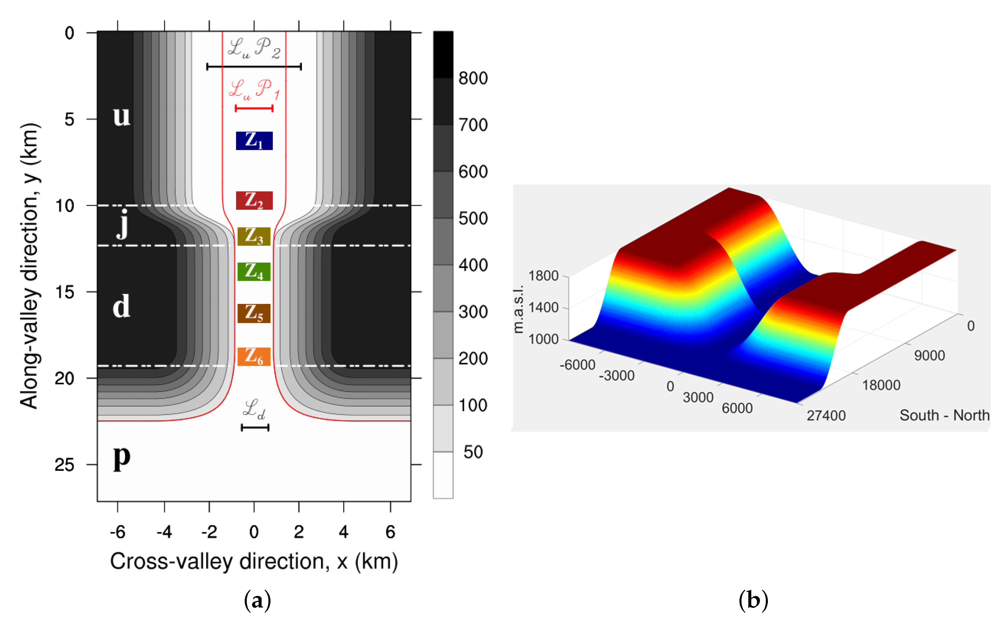
In the present work the Weather Research and Forecasting (WRF) model [24], version 3.4.1, is used to perform the numerical simulations. The model was run in a large-eddy simulation (LES) mode, as in Catalano and Cenedese (2010) [25], Wagner et al. (2014) [26] and Burns and Chemel (2015) [27] for instance. The model uses an Arakawa grid of type C and a terrain following coordinate system based on the dry-hydrostatic pressure. The 1.5-order turbulent kinetic energy (TKE) closure of Deardorff (1980) [28] is used to model subgrid-scale mixing, and it was modified following Scotti et al. (1993) [29] to account for the strong anisotropy of the grid along the slopes in the first vertical levels (see Section 2.3). The simulations use the same topography and initial conditions for the temperature and velocity fields as Arduini et al. (2017) [21]. A brief description of the configuration of the simulations is presented below.

2.2. Topography

The topography is a U-shaped valley of varying width, composed of an upstream section, called U , extending from 0 to 10 km in the y-direction, a downstream section, D , extending from 13 to 19 km and a 3-km long junction, J , between these two sections. The downstream section opens on a plain, P . The difference between U and D lies in the width of the valley floor, which is larger in the upstream section than in the downstream one (see Figure 1).
The valley is symmetrical about the y = 0 plane. Along the valley axis (y-direction), the valley is 44 km long and opens on a plain on both sides. Only the southern part of the domain is considered in the present work (see Figure 1). The slopes in U and D have the same length along the x-direction (4230 m). The top of the slopes are terminated by plateaux whose extensions are long enough to prevent boundary-related issues. The valley floor is set at 1000 m above the sea level, and the plateau height is set to 800 m above ground level. A detailed description of the terrain is reported in [21].
Two different values are considered for the upstream-valley floor width, called L 𝓊 , either equal to 1440 m or 4140 m. The former topography is referred to as T1 and the latter as T2. The downstream valley-floor width ( L 𝒹 ) is the same in T1 and T2 and equal to 360 m so that the constriction ratio between the upstream and downstream sections is equal to 4 for T1 and 11.5 for T2. All other geometrical parameters in T1 and T2 are the same (see Figure 1).

2.3. Numerical Setup

Numerical simulations using either topography T1 or topography T2 were run, referred to as P1 and P2, respectively. For each simulation, a nested domain is used with horizontal resolution 270 m for the outer domain and 90 m for the inner domain. In the along- and cross-valley directions, the outer domain extends over 90 km using 332 grid points and over 30 km using 112 grid points, respectively, far enough so that the boundaries do not have any effect on the results inside the valley over the duration of the simulations. For the outer domain an open boundary condition has been imposed in the northern and southern boundaries, while a periodic boundary condition has been set for the eastern and western boundaries. Outputs from the outer domain were used to provide the boundary conditions for the inner domain, with no feedback from the inner to the outer domain. Along the vertical, the domain top was set to 12,000 m above sea level and the vertical resolution was defined to decrease with height, with the first mass point located at 1.7 m above the ground and 25 grid points in the first 100 m above the ground. As shown by Largeron & Staquet (2016) [30], a vertical resolution of at least 4 m close to the ground should be used to get a good agreement with 2-m temperature measurements recorded on the upper part of the Grenoble valley. Due to the horizontal resolution used, the simulations may be better described as a high-resolution mesoscale simulation [31].
A stable atmosphere with a constant positive vertical gradient of (virtual) potential temperature of 1.5 K km 1 associated with a buoyancy frequency N = 0.00715 s 1 was set at the initial time, with no wind prescribed. P1 and P2 simulations started one hour and a half before sunset (15:30 local time) on a winter day (21 December) and lasted for 6 h. Therefore, the atmosphere of a winter night under dynamically decoupled conditions with no synoptic flow was considered.
The surface physics was represented using the revised MM5 Monin–Obukhov surface layer scheme [32]. The Rapid Radiative Transfer Model [33] and the scheme proposed by Dudhia (1989) [34] were used to model radiative transfer for long-wave and short-wave radiation, respectively. The surface cover in this simulation was set to “grassland” and the skin temperature was initialized from an extrapolation of the temperature of the first three layers above the surface.

2.4. Passive Tracer Emission

In the present work, PM 10 is treated as a passive (i.e., non-reactive) tracer and deposition (both dry and wet) was neglected. A set of passive tracers was released from six different emission zones along the valley axis (see Figure 1a). The same number of tracers was released continuously in each zone at a constant rate equal to Q = 2.25 × 10 6 kg s 1 from the initial time during the simulation. A constant background concentration equal to 1.25 × 10 12 kg m 3 was set in the whole domain for each tracer.
The following notation is used to identify the six different tracers emitted in each of the simulations: T r P n i , where P n refers to the simulations (P1 or P2) and i, to the emission zone along the valley axis (1 ≤ i ≤ 6). For example, the tracer emitted in the fourth emission zone (green zone in Figure 1a) in simulation P2, will be denoted by T r P 2 4 .

3. Low Atmosphere Structure

3.1. Along-Valley Flow

In a typical winter day, after the evening transition an along-valley flow develops in the down-valley direction due to the pressure gradient generated by the difference in cooling of the lower part of the atmosphere within the valley and over the plain [35]. The temporal evolution of the vertical structure of the along-valley flow is displayed in Figure 2 at the end of the upstream section U , and at the center of the downstream section D for simulations P1 and P2.
For P1, from 60 to 200 min into the simulation (see Figure 2a), an up-valley flow is present in the first hundred meters above the ground. Although in P2 the flow behavior seems to be rather complex (Figure 2c), a clear up-valley flow is identified as well. The up-valley flow is deeper in P1 (about 250-m deep at 180 min) compared to P2 (100-m deep at 180 min), but this up-valley flow in P2 has a greater speed and lasts longer (until the end of the simulated period). To estimate the relative impact on mass flux of either up-valley or down-valley flow, the cumulative mass flux in the vertical direction at y = 10 km is displayed in Figure 3 for P1 and P2 at two different times (100 and 200 min). This cumulative mass flux represents the amount of mass transported at a given position y in the along-valley direction from the ground up to a given height above ground level. Figure 3 shows that at 100 min the shallower flow in P2 (solid red line in Figure 3) transports more mass in the up-valley direction than the deeper flow in P1 (solid blue line in Figure 3). By contrast, at 200 min (dashed lines in Figure 3), when the flow is well developed in the down-valley direction, the amount of mass exported from U below the height of the plateaux is larger in P1 than in P2 by more than 30%.
In the downstream valley section D , no up-valley flow is observed in P1 or P2 (see Figure 2b,d), but differences in the vertical structure of the flow for each simulation can be noted. For P1 after 150 min the speed of the flow reaches about 1.5 m s 1 and appears to be vertically quasi-homogeneous up to 600 m above ground level. It reaches a quasi-steady state at around 200 min when the along-valley flow in the upstream section U reverses from up-valley to down-valley (see Figure 2a). The development of the down-valley flow close to the ground takes longer in P2 (200 min, see Figure 2d) and its speed reaches about 1.5 m s 1 at 250 min only. Its vertical structure is not as homogeneous as in P1 because of the development of the up-valley flow in U (see Figure 2c,d). The particular behavior of the along-valley flow at these positions is well explained by the differences in the thermal structure of the atmosphere along the valley axis, presented in the next section.

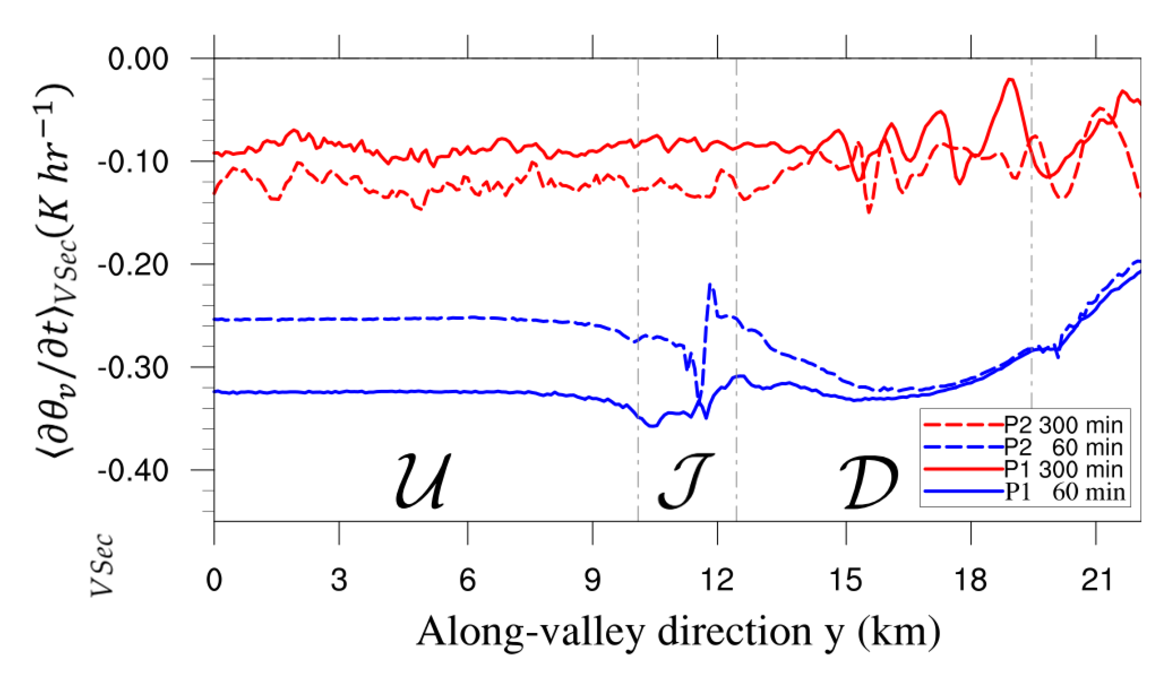
3.2. Thermal Structure

Figure 4 displays the change in potential temperature ( Δ θ ) between the initial time and 90 min into the simulation averaged over two different 1-km-long sections in the along-valley direction. The left and right panels in each frame of Figure 4 display Δ θ for a section center located at 10 km from the beginning of the valley, namely the exit of U , and at 16 km, namely half way along D , for P1 (frame a)) and P2 (frame b)). Horizontal white lines indicate the top height of the CAP (denoted by C A P t o p ), defined as in Burns and Chemel (2015) [27] by the local minimum of the vertical gradient of potential temperature above the ground-based inversion layer, averaged over the valley floor.
The CAP is shallower in U than in D for P1 and P2, the difference in CAP heights between the two valley sections being more pronounced for P2 than for P1. These differences are explained by the differences in the valley volume of each section. Since the length of the slopes are the same in U and D for P1 and P2, the mass flux from the slopes to the valley center is almost equal for any position along the valley (not shown). Thence, the smaller volume of D is filled with cold air from the slopes more rapidly and over a greater depth than the larger volume of U . As a result, the depth of the CAP is greater in D than in U (see Figure 4).
The average of the cooling rate over a cross-valley section extending up to the plateaux height is displayed in Figure 5. Differences in the cooling rate along the valley result in variations in temperature, which drive a pressure gradient and hence an along-valley flow. Since the vertical profile of temperature is the same for P1 and P2 at the initial time, the differences in the cooling rate between P1 and P2 must be attributed to the along-valley orographic difference between the two simulations. At 60 min, the cooling rate in U is lower in P2 than in P1 since the same amount of cold air is filling a larger valley volume as illustrated by the shallower CAP in P2. By contrast, in D the average cooling rate is similar for P1 and P2, as expected since the valley volume is the same. However, the region near J (between 13 and 16 km along y) in P1 cools relatively faster because of the greater export of near-surface cold air from D to U . At 300 min the flow is in a quasi-steady state for both P1 and P2, significantly reducing the differences in the thermal structure along the system due to the variations of the valley width [21]. As a result, the cooling rate along the valley axis is more homogeneous in its interior and a pressure gradient between the core of the valley and the plain is observed, which results in the down-valley flow recorded throughout the system.

4. Stagnation and Ventilation Zones

In this section, the effect of wind dynamics on the dispersion of passive scalars is identified by tracking areas prone to stagnation, recirculation and ventilation using the methodology developed by Allwine and Whiteman (1994) [23].

4.1. Summary of the Methodology Proposed by Allwine & Whiteman (1994)
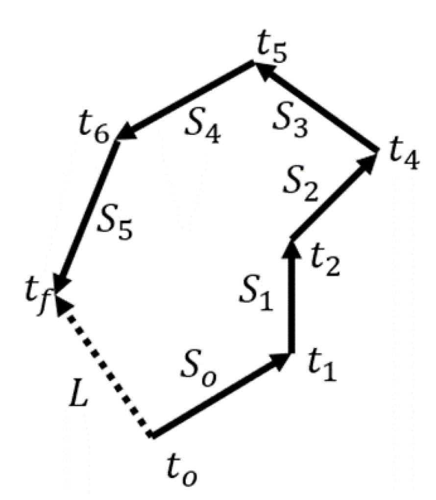
The methodology proposed by Allwine and Whiteman (1994) aims at characterizing the recirculation, stagnation and ventilation zones from time series of the horizontal velocity components at a fixed location (say at a mast). Let τ be the length of the time series and T the sampling interval of the series (or a time period, much smaller than τ , over which the data are averaged). The first step is to compute the flow speed and direction, U i and D i , respectively, the index i varying between 1 and τ / T . Allwine and Whiteman (1994) defined two main quantities to characterize the stagnation and ventilation zones induced by the velocity field, namely:
  • the time series S i , where S i is the virtual distance that an air parcel would travel during the time period T, assuming the air parcel does not experience any change in speed or direction during this time period, that is S i = T U i . Over the time τ , the parcel has travelled the virtual distance S = i = 1 n S i , where S is the wind run. The effective distance travelled by the fluid particle over time τ is denoted by L (see Figure 6).
  • the recirculation index R defined by:
    R = 1 L S .
    R quantifies the recirculation character of the flow: when R tends to 1, an air parcel following the flow may have travelled some distance, but its final position remains close to the initial position, meaning that it has experienced recirculation. Conversely, if R tends to 0, an air parcel is continuously moving away from its initial position; i.e., it has experienced ventilation (if S is large enough).
To classify the local transport properties of the velocity field, critical values for S and R (denoted by S c , S c v , R c and R c v ) are defined such that:
  • if S S c in a given zone, this zone is defined as a stagnation zone;
  • if R R c in a given zone, this zone is defined as a recirculation zone.
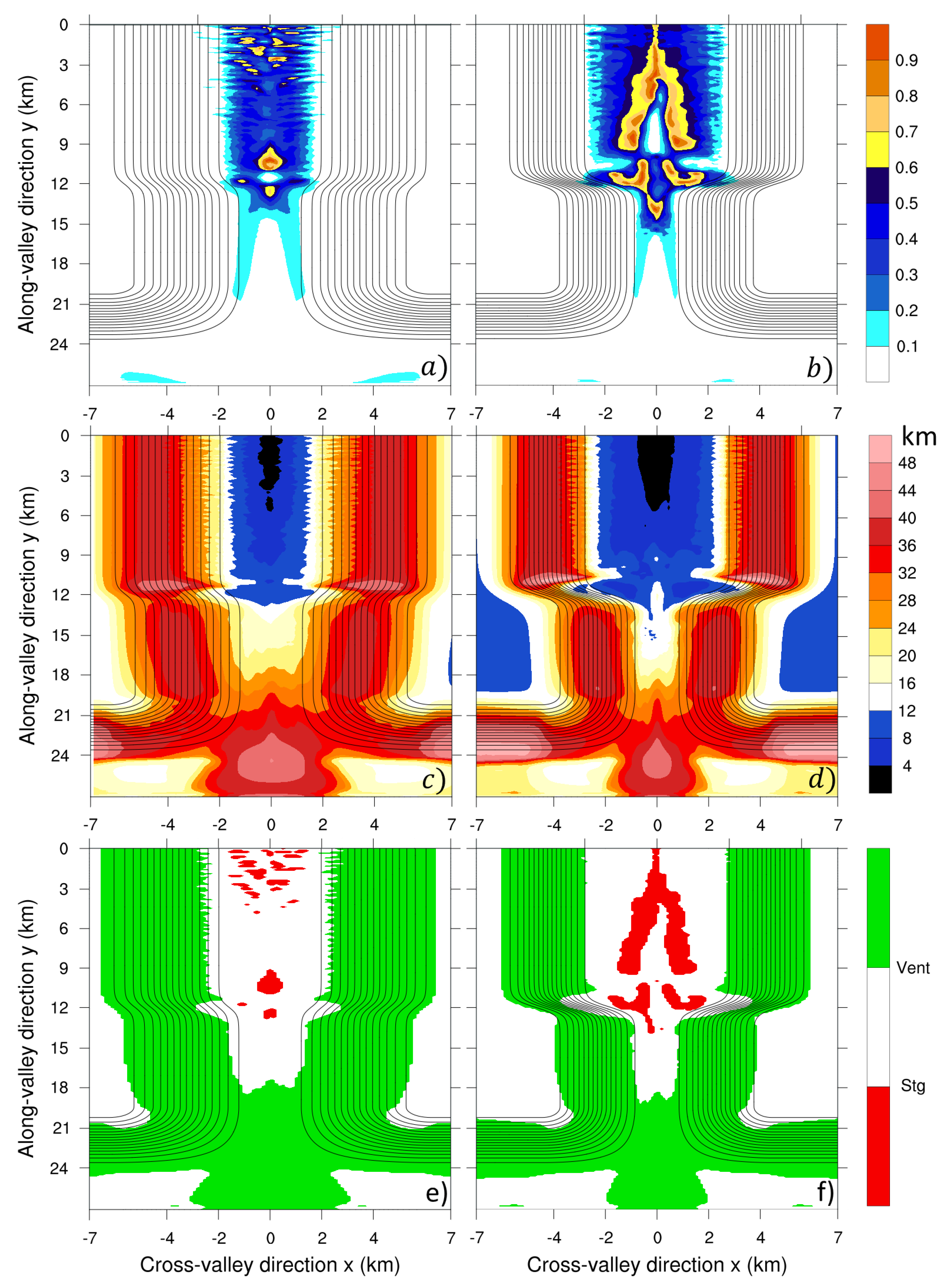
  • if R R c v and S S c v in a given zone, this zone is defined as a ventilation zone (green color in Figure 7e,f).
Largeron (2010) [36] added an additional class to better track zones prone to high tracer concentration,
  • if R R c and S S c , this zone is defined as a critical stagnation zone (red color in Figure 7e,f).
In the present work, Allwine and Whiteman’s methodology has been implemented by considering the three components of the velocity field, in order to account for the presence of valley slopes in the computation of the wind run S. The flow speed and direction are now spatial fields which we average over the first 30 m above the ground. Therefore, the wind run S and R are (time independent) spatial fields as well. The length τ was set to the simulated period (that is six hours) and T was set to 15 min. No turbulence transport is considered in the methodology since over the time scale considered ( τ = 6 h), transport by advection is dominant. Following [23], R c and R c v were set to 0.6 and 0.2 , respectively. Values for S c and S c v depend on the time interval τ , the flow speed and the orography, among other factors. In the present case, S c was set to 12 km, which represents 25 % of the maximum value of S computed from the results of the simulations (see Figure 7c,d) and S c v was set to 24 km.

4.2. Recirculation, Stagnation and Ventilation Zones

The zones prone to recirculation, stagnation or ventilation are now tracked for simulations P1 and P2.
Recirculation zones in simulation P1 are localized in the upstream-valley section, close to the exit of U and close to the beginning of the valley, and are of very limited extent (see Figure 7a). For P2 several recirculation zones are identified (see Figure 7b), in section U with a quasi-symmetric shape about the valley axis, and in the junction J , the latter zones possibly playing an important role in blocking the transport out of U .
Conversely, for the wind run S, the values and distribution over the domain are very similar in P1 and P2 (see Figure 7c,d). S reaches a maximum value of about 48 km at the exit of D and a minimum value close to 4 km in the core of U . Stagnation zones are found in U and J only (ignoring the plateaux region for P2).
Using the threshold values discussed in the previous subsection, the zones prone to critical stagnation and ventilation for each simulation are displayed in Figure 7e,f. Note that the recirculation zones are always detected in the stagnation zones (values of S less than 12 km), implying that the recirculation zones displayed in Figure 7a,b for P1 and P2 are also critical stagnation zones prone to high tracer concentration. By contrast, the slopes and the exit of the valley system, where a jet is detected, are ventilation zones. No ventilation zone is found in the valley core, which suggests that for tracers emitted close to the ground the whole system behaves as a trapper. This is particularly true for P2, where the largest recirculation zones are detected.
For P1, the recirculation zone detected away from the beginning of the valley corresponds to the position where the flow coming from the slope at the junction diverges between the U and D valley sections during the first 200 min of the simulated period. Due to the greater change in the cross-sectional area between U and D for P2, the flow dynamics are more complex than for P1 and a more detailed inspection is required.
Figure 8 displays a zoom on the zone where the recirculation zones for P2 are detected and shows streamlines averaged in time for three different time periods and over the first 30 m above the valley bottom. Between 60 and 120 min after the initial time (see Figure 8a), the air coming from the slopes converges at the center of the valley floor and flows in the up-valley direction, creating counter-rotating eddies near the end of U section and a recirculation zone close to the junction. The divergence of the along-valley flow near the end of U section also favors the creation of such a recirculation zone.
This zone is also visible between 120 and 180 min (see Figure 8b) while an up-valley flow is established throughout U . At the beginning of D the flow starts to flow down-valley (close to y = 15 km), which contributes to the creation of the most southern recirculation zone. Between 240 and 300 min the well-developed up-valley flow pushes the stagnant air up-valley into U (see Figure 8c). The stagnant air, advected towards the beginning of the valley by the up-valley flow, recirculates at the bottom of the slopes towards the center of the valley floor (flowing down-valley). This creates a quadrupole flow structure at the valley floor with a stagnation zone at the very center of U .

5. Transport of Passive Tracers

5.1. Horizontal Distribution of Tracers in the Lower Atmosphere

Figure 9 shows contour plots at the end of the simulated period of the normalized tracer concentration emitted at two different locations for both P1 and P2. Data from each plot has been normalized using the maximum concentration for each tracer, note that all tracers are independent from each other and this maximum value is different for all of them. Blue lines indicate the regions where critical stagnation is identified. Tracer T r P 1 1 (see Figure 9a) spreads throughout the valley floor; however, a small fraction of the mass of the tracer (compared to the mass of tracer remaining in U ) is transported from U to D . The maximum tracer concentration co-locates well with the critical stagnation zones at about 10 km from the beginning of the valley.
Tracer T r P 1 3 (see Figure 9b), emitted further down-valley, displays higher concentrations than T r P 1 1 at the end of the simulated period. Its emission zone is located at the exit of U (near a ventilation zone), but it coincides with the location of a recirculation zone. The proximity of the emission zone and the recirculation zone creates a localized region of high concentration at about 12 km, which afterwards is ventilated down valley.
The dynamics for P2 is, in general, more complex than for P1 and so is the evolution of the tracers. Figure 9c shows that there is almost no transport of tracer T r P 2 1 in the down-valley direction (a very small quantity of tracers is able to leave the section at the end of the simulated time period, see Figure 10e) because of the effect of the up-valley flow in the region where it is emitted. The air is transported in the up-valley direction and diverges towards the slopes as it encounters the more stagnant air further upstream. There is a good agreement between the zones of high tracer concentration and the critical stagnation zones (blue lines in Figure 9c). Tracer T r P 2 3 (see Figure 9d) is emitted at J just in between the stagnation zones found there, and so it remains trapped close to its emission zone. Note that even though it is released in a local non-stagnant zone, it remains confined near the emission zone because it is surrounded by stagnant air. The latter suggests that relationship between zones of high concentration of tracers and areas marked as prone to stagnation should be considered with caution, the variability in the concentration of air pollutants is not only a function of atmospheric dynamics; location and emission rates also play an important role in the problem.

5.2. Ventilation Efficiency

To quantify the effect of D section on the ventilation of the tracers emitted in U section (presented briefly in the previous section), the mass of each tracer within the volumes of U , J , D and P , relative to its mass emitted from the initial time to time t, denoted by R M , is analysed. R M is defined by:
R M = V i C · d V Q · t ,
where C is the tracer concentration in k g m 3 , V i represent volumes of valley segments with i = U , J , D , P and Q is the constant emission rate of the tracer. The top surface of each volume V i is set by the height of the plateaux (that is 1800 m a.s.l.).
T r P 1 1 is confined within V U for the first four hours because the emission zone is located on a stagnation zone (see Figure 10a). This applies also to the other tracer emitted in V U ( T r P 1 2 ). As soon as the down-valley flow is fully developed in U (at about 240 min) R M starts to decrease steadily. At 300 min the mass within V U has already decreased at about 55% of the mass emitted. The tracer is transported along the system of valley segments and reaches the plain by the very end of the simulated period (i.e., within two hours).
For T r P 2 1 (see Figure 10e) the effect of stagnation is greatly amplified, as was shown in the previous section. The tracer is transported to J after 300 min, and its mass within V U decreases by just around a 10% by the end of the simulated period (i.e., within one hour). This result suggests that the narrow constriction strongly affects the ventilation of the tracers from this section. The mass of tracer transported out of U is reduced by about 60% between P1 and P2 by the end of the simulated period.
The behavior of T r P 1 3 emitted at the junction between the two valley sections (see Figure 10b) is not very different to that of T r P 1 1 . The mass of tracer within V J appears to remain constant until two hours of simulation. From this time, the tracer starts to flow downstream with some transport upstream for two more hours as a result of the divergence of the flow within the junction. After about 210 min from the beginning of the simulation the flow in the whole domain is completely down-valley (see Figure 2a,b) driving the tracers out of the entire valley, which is consistent with the linear decrease of R M within V D and a continued linear increase of R M within V P for the last two hours of simulation. The transport of T r P 2 3 from J to D is delayed further (see Figure 10f) because the up-valley flow in V U persists for longer (see Section 3.1). By the end of the simulated period the mass of T r P 2 3 within V J is almost three times larger than what have left of T r P 1 3 in V J .
Two tracers/emission zones are considered for the volume V D to better characterize the zone. T r P n 4 , emitted 14 km from the beginning of the valley, reaches first a neighboring section after about 80 min. Initially a predominantly up-valley flow drives something close to the 30% of the total mass of tracer through V J . Afterwards a down-valley flow establishes quickly and transports the tracer out of the valley (which eventually reaches the plain after three hours of simulation). At the end of the simulated period, about 80% of the total emitted tracer mass has left the valley (that is in V P ). Stagnation is amplified for P2 because the up-valley flow is stronger than for P1. The transport up-valley is greater; an equivalent mass of about the 25% of the total mass emitted reaches V U at the end of the first three hours of simulation. When the flow changes direction and tracers are transported in the down-valley direction, nonetheless the mass of tracer in V U and V J combined at the end of the simulation is about the 25%. Regardless of the ventilation during the last part of the simulation, almost twice as much mass remains close to the release zone for P2 compared to P1.
Tracers T r P 1 5 and T r P 2 5 emitted half way along D display a very similar behavior since they are advected in the down-valley direction once the along-valley flow develops (around 120 min). The latter indicates that the dynamics in D away from J is independent of the geometry of the neighbor valley for the range of geometrical parameters considered in this work.
R M provides information about the location of the tracers through the different sections of the valley system, but a quantification of the time required to ventilate each of the sections of the valley is still necessary. A synthetic account of the ventilation character of the different sections of the valley system can be provided by computing the residence time of the tracers at each section. The residence time can be seen as a volume parameter that aims to describe the general exchange characteristics of a control volume leaving aside the identification of the underlying physical processes or their spatial distribution [37]. The residence time T is defined simply as:
T = m t o t a l f
where m t o t a l is the total mass stored in the control volume at the time when the calculation is performed and f is the mass fluxes through the boundaries. When the fluxes out of the control volume are near zero or into the volume, T will tend to infinity (i.e., the tracers will remain always inside the control volume). On the other hand, if the tracer flux is large compared with the tracer mass in the volume, the tracer residence time will tend to zero.
Figure 11 displays a compilation of the tracer residence time for three tracers. The tracer released at the center of V D ( T r P 1 5 ) is mainly subjected to ventilation, the residence time reaches a quasi-steady state ( T ≈ 10 0 h) once the along-valley flow is established after two hours of simulation. This value is used as a reference for ventilation residence time and is denoted by T v . Note that T v corresponds to an average flow speed in this valley section of about 2.6 m s 1 , which is consistent with what was presented in Figure 2b for the last two hours of simulation. The oscillatory behavior of T (of about ±15 min) may be a consequence of the oscillation in the flow speed magnitude previously encountered in drainage valleys similar to V D [16]. The residence time for T r P 1 3 does reach a steady state corresponding to pure ventilation about one hour later than for T r P 1 5 . Conversely, for T r P 1 1 the value of T at the end of the simulation was two times larger than the one of T v (please be aware of the logarithmic scale of the vertical axis in Figure 11), indicating that the stagnation character of V U is noted until the end of the simulated period for P1. Even with the zones of stagnation detected for P1, the system as a whole could be seen as a drainer valley due to the ventilation character shown in Figure 11.
As it was mentioned before, the wind dynamics in the last portion of V D is very similar for both P1 and P2 (see Figure 2b,d). Tracer T r P 2 5 has a very similar behavior than T r P 1 5 , T quickly reaching a quasi-steady state near the value of T v and remaining thus until the end of the simulation. Tracer T r P 2 3 starts to be ventilated at about 2 h of simulation, but due to the complexity of the system after four hours T increases, reflecting the change of direction of the along-valley flow by transporting back to V J the tracers previously advected in the up-valley direction. Afterwards this model run seems to reach a stable regime with T v almost three times larger than T v , implying that at least by the end of the simulated period it does not show ventilation of tracers. Finally, the residence time of T r P 2 1 at V U clearly expresses the weak ventilation shown above. At the end of the simulation it displays a T of about 10 h, indicating that this portion of valley is characterized as an accumulation zone.
Arduini et al. (2017) [21] following the work of Whiteman et al. (1996) [38] indicates that P1 is considered to be a drainer valley, and P2 can be considered to be a trapper. From the tracer experiment presented here it is possible to infer that for P2 the valley as a whole could not be considered to be a trapper due to the strong ventilation shown at the end of V D .

6. Summary and Conclusions

Numerical simulations were performed to examine the response of the transport of air pollutants, modelled as passive tracers, to orographic variations along the axis of an idealized version of an Alpine valley during wintertime after the evening transition. A system of two valley sections sharing the same axis, with one of the sections opening on a narrower valley, which opens on a plain, is considered. Two sets of simulations were considered, named P1 and P2 for which the valley-floor width of the downstream valley section is the same ( L 𝒹 = 360 m), but that of the upstream-valley section ( L 𝓊 ) was set to 1440 m ( L 𝓊 / L 𝒹 = 4 ) and 4230 m ( L 𝓊 / L 𝒹 = 11.5 ), respectively. The transport of passive tracers across the domain has been analyzed for six different tracer releases along the valley axis. The main conclusions of this work can be summarized as follows:
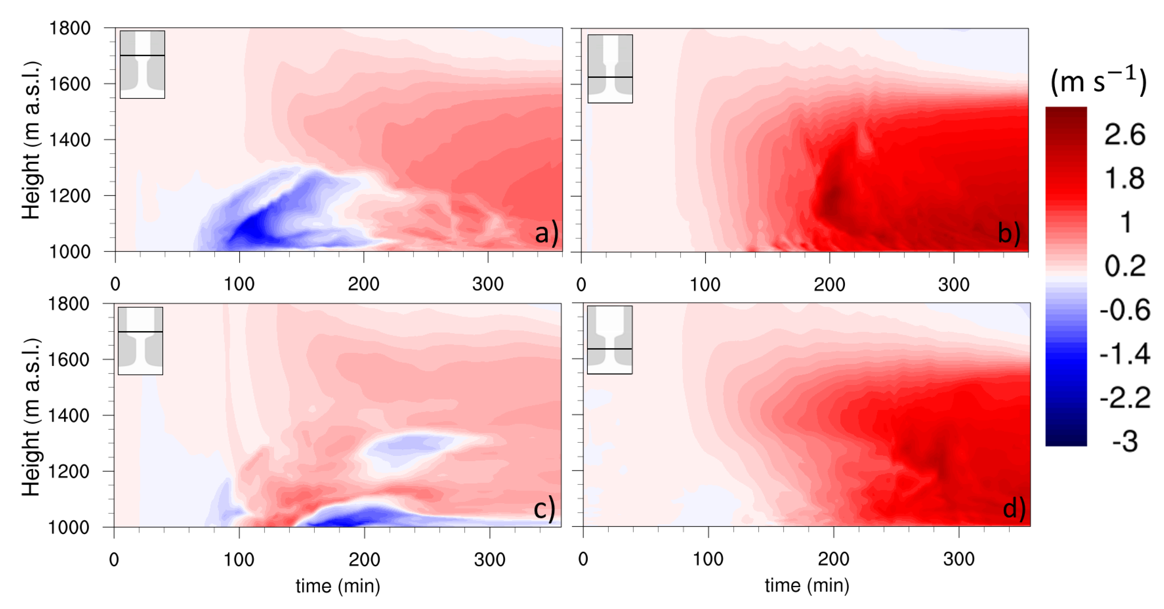
  • The change in the thermal structure of the atmosphere within the different sections of the valley and the plain generates a horizontal pressure gradient that leads to the development of an along-valley flow. For P1 it is up-valley in the upstream-valley section during the first three hours of simulation and then reverses in the downstream direction for the rest of the simulated time period (six hours). For P2 a faster up-valley flow persists in the upstream-valley section until the end of the simulated period. These differences in the dynamics between P1 and P2 translate into differences in the horizontal mass flux in the upstream-valley section: after 3 h of simulation it is 1.5 times larger for P1 than for P2 (see Figure 3).
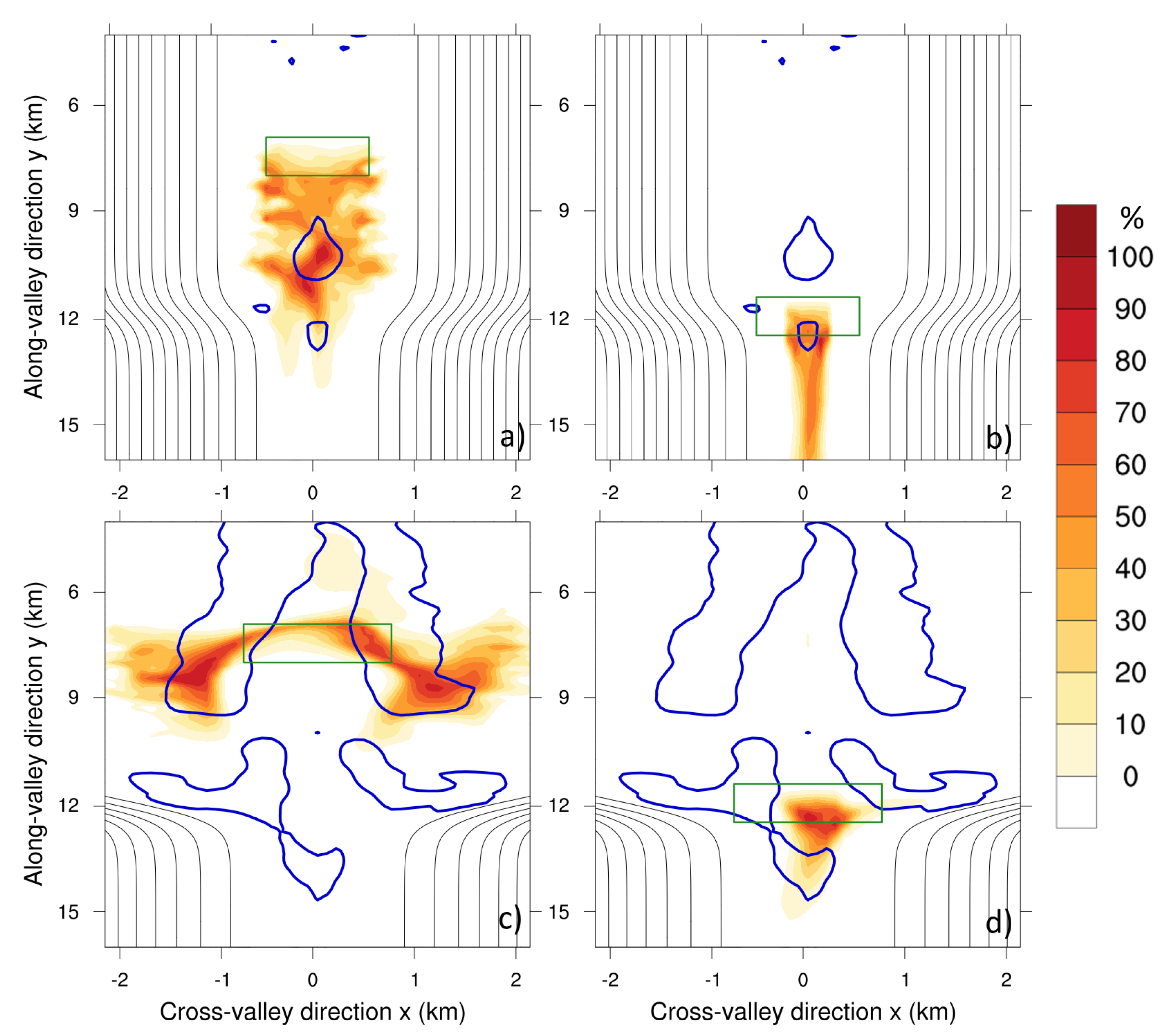
  • The methodology proposed by Allwine and Whiteman (1994) [23] to predict locations prone to ventilation, stagnation and recirculation was evaluated and found to work well for predicting areas with high tracer concentration. Indeed, the zones where critical stagnation is detected agree well with zones of high tracer concentration (see Figure 9). However, the relationship between areas identified as prone to stagnation and the zones of high tracer concentration should be considered with caution since the variability in the concentration of air pollutants is not only a function of atmospheric dynamics but also of the emission location and rate, as shown in Figure 9d.
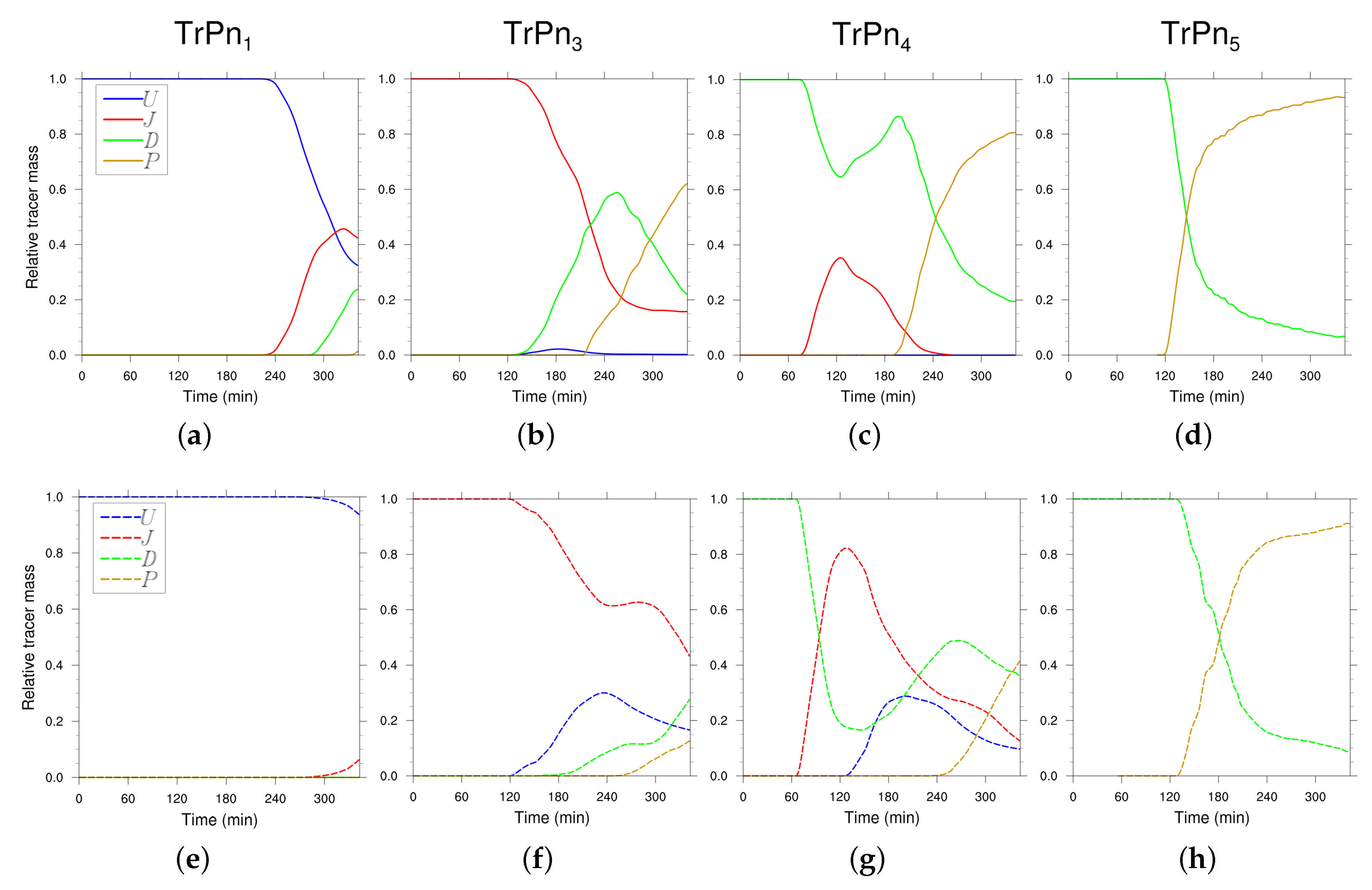
  • The sizable change in the cross-sectional area between the upstream ( U ) and downstream ( D ) valleys affects atmospheric dynamics, and hence tracer transport across the domain. The export of tracers out of U is reduced by about 50% for P2 compared to that for P1 (see Figure 10a,e). Intra-valley transport of tracers is also reduced in D . By the end of the simulated period 80% of the total mass emitted for tracer T r P 1 4 (at the beginning of D ) has been transported out of the valley section while for tracer T r P 2 4 (which is emitted at the same position but for P2) only 40% of the total mass emitted have left the valley section (see Figure 10c,g).
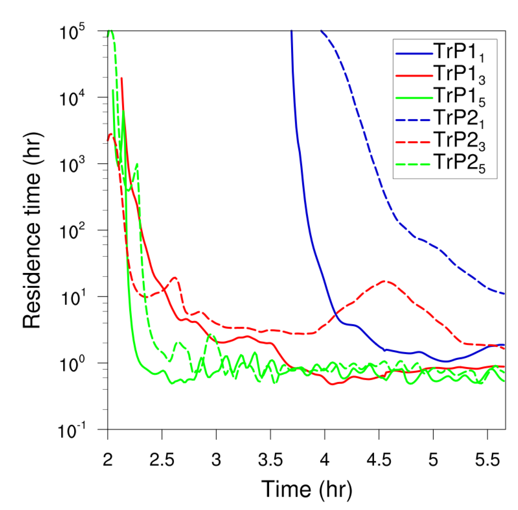
  • The ventilation efficiency within the different sections of the valley system was quantified by a residence time. For P1 the residence time within U (about two hours) is more than twice that within D (about one hour) at the end of the simulated time period (Figure 11). On the other hand, this difference is more pronounced for P2, where the ventilation efficiency for U (about 10 h) is reduced by more than a factor of ten when compared to that of D (about one hour).

Author Contributions

J.Q.-D. and G.A. conducted and designed the numerical simulations. J.Q.-D., C.S. and C.C. designed the numerical experiment. J.Q.-D. performed the postprocessing of the results and prepared the manuscript. C.S. and C.C. revised and improved the manuscript.

Funding

This research received no external funding.

Acknowledgments

This work has been supported by a PhD grant provided by the Colombian Administrative Department of Science, Technology and Innovation, COLCIENCIAS. Numerical simulations were run on the French national HPC facilities at CINES.

Conflicts of Interest

The authors declare no conflict of interest.

References

  1. Gohm, A.; Harnisch, F.; Vergeiner, J.; Obleitner, F.; Schnitzhofer, R.; Hansel, A.; Fix, A.; Neininger, B.; Emeis, S.; Schäfer, K. Air pollution transport in an Alpine valley: Results from airborne and ground-based observations. Bound.-Layer Meteorol. 2009, 131, 441–463. [Google Scholar] [CrossRef]
  2. Silcox, G.D.; Kelly, K.E.; Crosman, E.T.; Whiteman, C.D.; Allen, B.L. Wintertime PM 2.5 concentrations during persistent, multi-day cold-air pools in a mountain valley. Atmos. Environ. 2012, 46, 17–24. [Google Scholar]
  3. Chemel, C.; Burns, P. Pollutant dispersion in a developing valley cold-air pool. Bound.-Layer Meteorol. 2015, 154, 391–408. [Google Scholar] [CrossRef]
  4. Largeron, Y.; Staquet, C. Persistent inversion dynamics and wintertime PM 10 air pollution in Alpine valleys. Atmos. Environ. 2016, 135, 92–108. [Google Scholar] [CrossRef]
  5. Jaffrezo, J.L.; Aymoz, G.; Delaval, C.; Cozic, J. Seasonal variations of the water soluble organic carbon mass fraction of aerosol in two valleys of the French Alps. Atmos. Chem. Phys. 2005, 5, 2809–2821. [Google Scholar] [CrossRef] [Green Version]
  6. Whiteman, C.D. Observations of thermally developed wind systems in mountainous terrain. In Atmospheric Processes over Complex Terrain; American Meteorological Society: Boston, MA, USA, 1990; pp. 5–42. [Google Scholar]
  7. Whiteman, C.D.; Hoch, S.W.; Horel, J.D.; Charland, A. Relationship between particulate air pollution and meteorological variables in Utah’s Salt Lake Valley. Atmos. Environ. 2014, 94, 742–753. [Google Scholar] [CrossRef]
  8. Chemel, C.; Arduini, G.; Staquet, C.; Largeron, Y.; Legain, D.; Tzanos, D.; Paci, A. Valley heat deficit as a bulk measure of wintertime particulate air pollution in the Arve River Valley. Atmos. Environ. 2016, 128, 208–215. [Google Scholar] [CrossRef] [Green Version]
  9. Allwine, K.J.; Whiteman, C.D. Ventilation of pollutants trapped in valleys: A simple parameterization for regional-scale dispersion models. Atmos. Environ. 1988, 22, 1839–1845. [Google Scholar] [CrossRef]
  10. Regmi, R.P.; Kitada, T.; Kurata, G. Numerical simulation of late wintertime local flows in Kathmandu valley, Nepal: Implication for air pollution transport. J. Appl. Meteorol. 2003, 42, 389–403. [Google Scholar] [CrossRef]
  11. Maurizi, A.; Russo, F.; Tampieri, F. Local vs. external contribution to the budget of pollutants in the Po Valley (Italy) hot spot. Sci. Total Environ. 2013, 458, 459–465. [Google Scholar] [CrossRef]
  12. Rotach, M.W.; Wohlfahrt, G.; Hansel, A.; Reif, M.; Wagner, J.; Gohm, A. The world is not flat: Implications for the global carbon balance. Bull. Am. Meteorol. Soc. 2014, 95, 1021–1028. [Google Scholar] [CrossRef]
  13. Serafin, S.; Zardi, D. Daytime heat transfer processes related to slope flows and turbulent convection in an idealized mountain valley. J. Atmos. Sci. 2010, 67, 3739–3756. [Google Scholar] [CrossRef]
  14. Colette, A.; Chow, F.K.; Street, R.L. A numerical study of inversion-layer breakup and the effects of topographic shading in idealized valleys. J. Appl. Meteorol. 2003, 42, 1255–1272. [Google Scholar] [CrossRef]
  15. Lehner, M.; Gohm, A. Idealised simulations of daytime pollution transport in a steep valley and its sensitivity to thermal stratification and surface albedo. Bound.-Layer Meteorol. 2010, 134, 327–351. [Google Scholar] [CrossRef]
  16. Quimbayo-Duarte, J.; Staquet, C.; Chemel, C.; Arduini, G. Dispersion of Tracers in the Stable Atmosphere of a Valley Opening onto a Plain. Bound.-Layer Meteorol. 2019. under review. [Google Scholar] [CrossRef]
  17. Wagner, A. Theorie und beobachtung der periodischen Gebirgswinde. Gerlands Beitr. Geophys. 1938, 52, 408–449. [Google Scholar]
  18. Steinacker, R. Area-height distribution of a valley and its relation to the valley wind. Contrib. Atmos. Phys. 1984, 57, 64–71. [Google Scholar]
  19. Vergeiner, I.; Dreiseitl, E. Valley winds and slope winds—Observations and elementary thoughtsBerg-und Tal-bzw. Hangwinde—Beobachtungen und grundsätzliche Überlegungen. Meteorol. Atmos. Phys. 1987, 36, 264–286. [Google Scholar] [CrossRef]
  20. McKee, T.B.; O’Neal, R.D. The role of valley geometry and energy budget in the formation of nocturnal valley winds. J. Appl. Meteorol. 1989, 28, 445–456. [Google Scholar] [CrossRef]
  21. Arduini, G.; Chemel, C.; Staquet, C. Energetics of deep alpine valleys in pooling and draining configurations. J. Atmos. Sci. 2017, 74, 2105–2124. [Google Scholar] [CrossRef]
  22. Li, J.; Atkinson, B. Transition regimes in valley airflows. Bound.-Layer Meteorol. 1999, 91, 385–411. [Google Scholar] [CrossRef]
  23. Allwine, K.J.; Whiteman, C.D. Single-station integral measures of atmospheric stagnation, recirculation and ventilation. Atmos. Environ. 1994, 28, 713–721. [Google Scholar] [CrossRef]
  24. Skamarock, W.C.; Klemp, J.B.; Dudhia, J.; Gill, D.O.; Barker, D.M.; Duda, M.G.; Huang, X.Y.; Wang, W.; Powers, J.G. A Description of the Advanced Research WRF, Version 3; Technical Report; Mesoscale and Microscale Meteorology Division, National Center for Atmospheric Research: Boulder, CO, USA, 2005. [Google Scholar]
  25. Catalano, F.; Cenedese, A. High-resolution numerical modeling of thermally driven slope winds in a valley with strong capping. J. Appl. Meteorol. Climatol. 2010, 49, 1859–1880. [Google Scholar] [CrossRef]
  26. Wagner, J.S.; Gohm, A.; Rotach, M.W. The impact of horizontal model grid resolution on the boundary layer structure over an idealized valley. Mon. Weather Rev. 2014, 142, 3446–3465. [Google Scholar] [CrossRef]
  27. Burns, P.; Chemel, C. Interactions between downslope flows and a developing cold-air pool. Bound.-Layer Meteorol. 2015, 154, 57–80. [Google Scholar] [CrossRef]
  28. Deardorff, J.W. Stratocumulus-capped mixed layers derived from a three-dimensional model. Bound.-Layer Meteorol. 1980, 18, 495–527. [Google Scholar] [CrossRef]
  29. Scotti, A.; Meneveau, C.; Lilly, D.K. Generalized Smagorinsky model for anisotropic grids. Phys. Fluids A Fluid Dyn. 1993, 5, 2306–2308. [Google Scholar] [CrossRef] [Green Version]
  30. Largeron, Y.; Staquet, C. The atmospheric boundary layer during wintertime persistent inversions in the Grenoble valleys. Front. Earth Sci. 2016, 4, 70. [Google Scholar] [CrossRef]
  31. Wyngaard, J.C. Toward Numerical Modeling in the Terra Incognita. J. Atmos. Sci. 2004, 61, 1816–1826. [Google Scholar] [CrossRef]
  32. Jiménez, P.A.; Dudhia, J.; González-Rouco, J.F.; Navarro, J.; Montávez, J.P.; García-Bustamante, E. A revised scheme for the WRF surface layer formulation. Mon. Weather Rev. 2012, 140, 898–918. [Google Scholar] [CrossRef]
  33. Mlawer, E.J.; Taubman, S.J.; Brown, P.D.; Iacono, M.J.; Clough, S.A. Radiative transfer for inhomogeneous atmospheres: RRTM, a validated correlated-k model for the longwave. J. Geophys. Res. 1997, 102, 663–682. [Google Scholar] [CrossRef]
  34. Dudhia, J. Numerical study of convection observed during the winter monsoon experiment using a mesoscale two-dimensional model. J. Atmos. Sci. 1989, 46, 3077–3107. [Google Scholar] [CrossRef]
  35. Zardi, D.; Whiteman, C.D. Diurnal mountain wind systems. In Mountain Weather Research and Forecasting; Springer: Dordrecht, The Netherlands, 2013; pp. 35–119. [Google Scholar]
  36. Largeron, Y. Dynamique de la Couche Limite Atmosphérique Stable en Relief Complexe. Application aux épisodes de Pollution Particulaire des Vallées Alpines. Ph.D. Thesis, Université de Grenoble, Grenoble, France, 2010. [Google Scholar]
  37. Monsen, N.E.; Cloern, J.E.; Lucas, L.V.; Monismith, S.G. A comment on the use of flushing time, residence time, and age as transport time scales. Limnol. Oceanogr. 2002, 47, 1545–1553. [Google Scholar] [CrossRef] [Green Version]
  38. Whiteman, C.D.; McKee, T.B.; Doran, J. Boundary layer evolution within a canyonland basin. Part I: Mass, heat, and moisture budgets from observations. J. Appl. Meteorol. 1996, 35, 2145–2161. [Google Scholar] [CrossRef]
Figure 1. (a) Contours of the terrain height in meters from the valley bottom for topography T2; the contours are plotted every 50 m, the first contour of topography T1 being indicated with a red line. The topography is oriented north-south in the y-direction, the valley being symmetric along the y = 0 -plane. The valley is composed of three main sections, an upstream section, called U , a downstream section D and a plain P at the end of the valley; sections U and D are linked by a junction J . Six different emission zones are set along the valley axis continuously releasing in each zone the same amount of tracers at a constant rate equal to Q = 2.25 × 10 6 kg s 1 from the initial time during the simulation. The notation used for each tracer is explained in Section 2.4. (b) Three-dimensional representation of topography T2. Frames (a,b) display the southern part of the domain.
Atmosphere 10 00225 g001
Figure 2. Hovmöller diagrams of the evolution of the along-valley flow speed for P1, at 10 km (a) and 16 km (b) from the beginning of the valley; and for P2, at 10 km (c) and 16 km (d) from the beginning of the valley. The flow speed is averaged over the valley-floor width in x-direction, and over 1 km along the y-direction. Positive (red) values correspond to a down-valley flow while negative values (blue) to an up-valley flow. The y-position of either figure is indicated in the sketch in the upper-left corner of each panel.
Atmosphere 10 00225 g002
Figure 3. Cumulative mass flux across a vertical surface perpendicular to the valley axis located at 10 km from the beginning of the valley for P1 (blue lines) and P2 (red lines) at 100 (solid lines) and 200 min (dashed lines) into the simulation (with a 10 min average about these times). The calculation has been limited in the cross-valley direction to the width of the valley floor to avoid the effect of volume increase with height.
Atmosphere 10 00225 g003
Figure 4. Vertical cross sections of the change in the potential temperature ( Δ θ ) with respect to the initial condition averaged over 1 km along the y-direction and over 10 min about 90 min into the simulation for P1 (a), and P2 (b). Each frame is divided in two panels, the left panel corresponding to the exit of the upstream-valley U (10 km) and the right panel corresponding to the mid part of the downstream valley D (16 km). White lines represent an estimate of the CAP height at each section.
Atmosphere 10 00225 g004
Figure 5. Average of the cooling rate over a cross-section extending up to the plateaux height ( θ v / t V S e c ) at the end of the first hour (blue line) and at the end of fourth hour (red line) of simulation (with a 10 min average) for P1 (solid lines) and P2 (dashed lines). Vertical grey dashed lines stand for the end of each section of the valley.
Atmosphere 10 00225 g005
Figure 6. Sketch of the definitions of the wind run ( S i ) and of the transport distance (L). Each segment S i is computed using an average over the time interval T equal to 15 min. Note that the end of each arrow in the figure corresponds to a time, not a point in space. Adapted from [23].
Atmosphere 10 00225 g006
Figure 7. Contour plots of the recirculation factor (R, top row), contour plots of the wind run (S, middle row) and zones prone to critical stagnation and ventilation (bottom row) for P 1 (a,c,e) and P 2 (b,d,f) simulations overlaid with contour lines of the terrain height using a 50 m interval. Each point in the domain has been averaged over 15 min and over the first 30 m above the ground level. The unit for S is km.
Atmosphere 10 00225 g007
Figure 8. Zoom on the upper part of the valley for P2 displaying streamlines overlaid with contour lines of the terrain height using a 50 m interval. The velocity field is vertically averaged over the first 30 m above the valley bottom and averaged in time over (a) 60–120 min, (b) 120–180 min and (c) 240–300 min.
Atmosphere 10 00225 g008
Figure 9. Contour plot of the normalized tracer concentration (percentage) at the end of the simulation (averaged over the last 15 min of simulation) overlaid over contour lines of the terrain height using 50 m intervals between them for (a) T r P 1 1 , (b) T r P 1 3 , (c) T r P 2 1 and (d) T r P 2 3 averaged over the first 30 m along the vertical. All figures are normalized with the maximum concentration for each of the tracers plotted, which is different in all the cases. Blue lines correspond to the locations where the critical stagnation zones are located (Figure 7e,f). Green rectangles represent the emission zones for each of the tracers.
Atmosphere 10 00225 g009
Figure 10. Time series of the relative tracer mass ( R M ) at the different control volumes in the system ( V U , V J , V D and V P ) for tracers T r P n 1 released at U (a and e), T r P n 3 released at J (b and f), T r P n 4 released at the beginning of D (c and g) and T r P n 5 released at the center of D (d and h). Note that n = 1 for P1 and n = 2 for P2. Solid lines represent values of P1 (top row), while dashed lines stand for P2 (bottom row). The location of the emission source of each of the tracers is presented in Figure 1a.
Atmosphere 10 00225 g010
Figure 11. Time series of the residence time ( T ) of tracers T r P n 1 (blue lines, tracer released at U ), T r P n 3 (red lines, tracer released at J ) and T r P n 5 (green lines, tracer released at D ). Note that n = 1 for P1 and n = 2 for P2. Solid lines represent values of P1, while dashed lines stand for P2. The location of the source of each of the tracers is presented in Figure 1a. The control volume used to calculate the residence time is the volume of the valley segment for each of the tracer emission sites up to the height of the plateaux.
Atmosphere 10 00225 g011

