Passive Earth Observations of Volcanic Clouds in the Atmosphere


Abstract
:
1. Introduction
2. Satellite Orbits and Sensors
2.1. Polar Orbits
2.2. Geostationary Orbits
2.3. Sensors
3. Methods–Volcanic Ash Detection and Retrieval
3.1. Physical Principles of Ash Detection in the Infrared
3.2. Modelling Radiative Transfer in Ash Clouds
3.3. Heuristic Model
3.4. Solving the Heuristic Model
3.5. Correcting for Water Vapour Effects
- (1)
- the clear-sky surface temperature ,
- (2)
- the cloud-top temperature ,
- (3)
- the clear-sky value of the water vapour correction, and
- (4)
- the ratio of extinction coefficients that governs the magnitude of the “U-shaped” distribution of negative differences.
- . This is easily estimated by finding the maximum value of occurring in the data.
- . This is more difficult to estimate from the data, because the lowest value may not necessarily correspond to the volcanic cloud. However, provided an area in close proximity to the suspect cloud can be delineated it may be reasonable to assume that the lowest value is the cloud-top temperature.
- Water vapour correction. An empirical relation [32] between the precipitable water in an atmospheric column and the brightness temperature difference () is used to estimate the water vapour effectwhere , and is an arbitrary normalisation constant assigned a value of 320 K. The free parameter b essentially determines the value of the water vapour effect on at the maximum value of . Hence b can be determined directly from the image data, allowing realistic flexibility on the size of the water vapour correction determined by this semi-empirical approach.
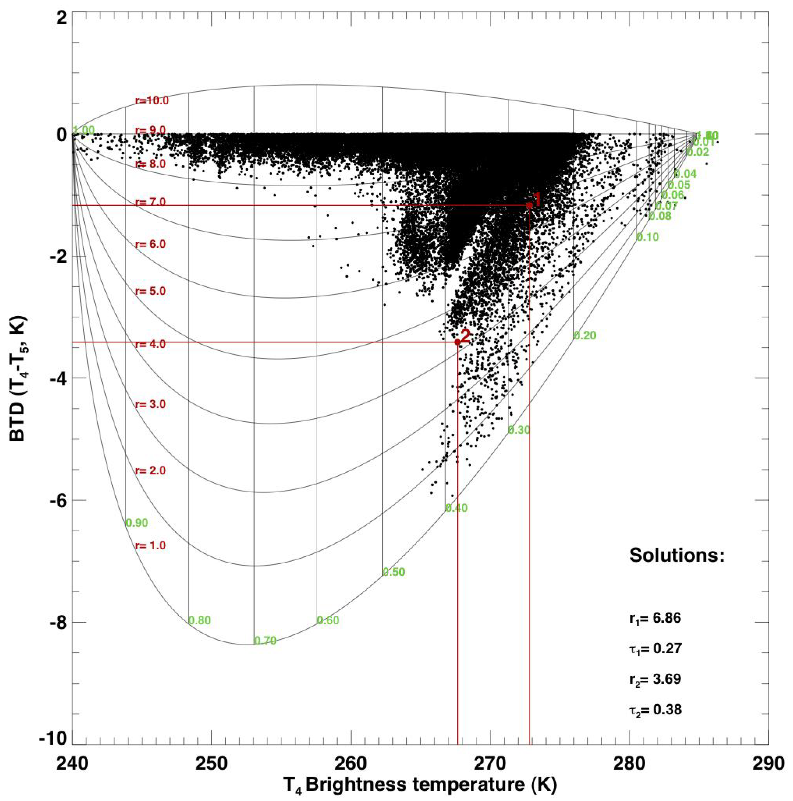
- . Theoretical estimates of suggest a value of around 0.7. A method for estimating , and simultaneously has been developed by using the distribution of vs. . The distribution is first histogrammed (or binned) into intervals of 0.5 K in . Then, the lowest values in each bin are found and a curve is generated giving the outline of the distribution. The curve is smoothed and fitted using a nonlinear least squares model. The model has three parameters, viz.: , and that can be estimated from the fit.
4. Complex Radiative Transfer Model
4.1. Refractive Index and Composition
4.2. Size Distribution
4.3. Optical Depth
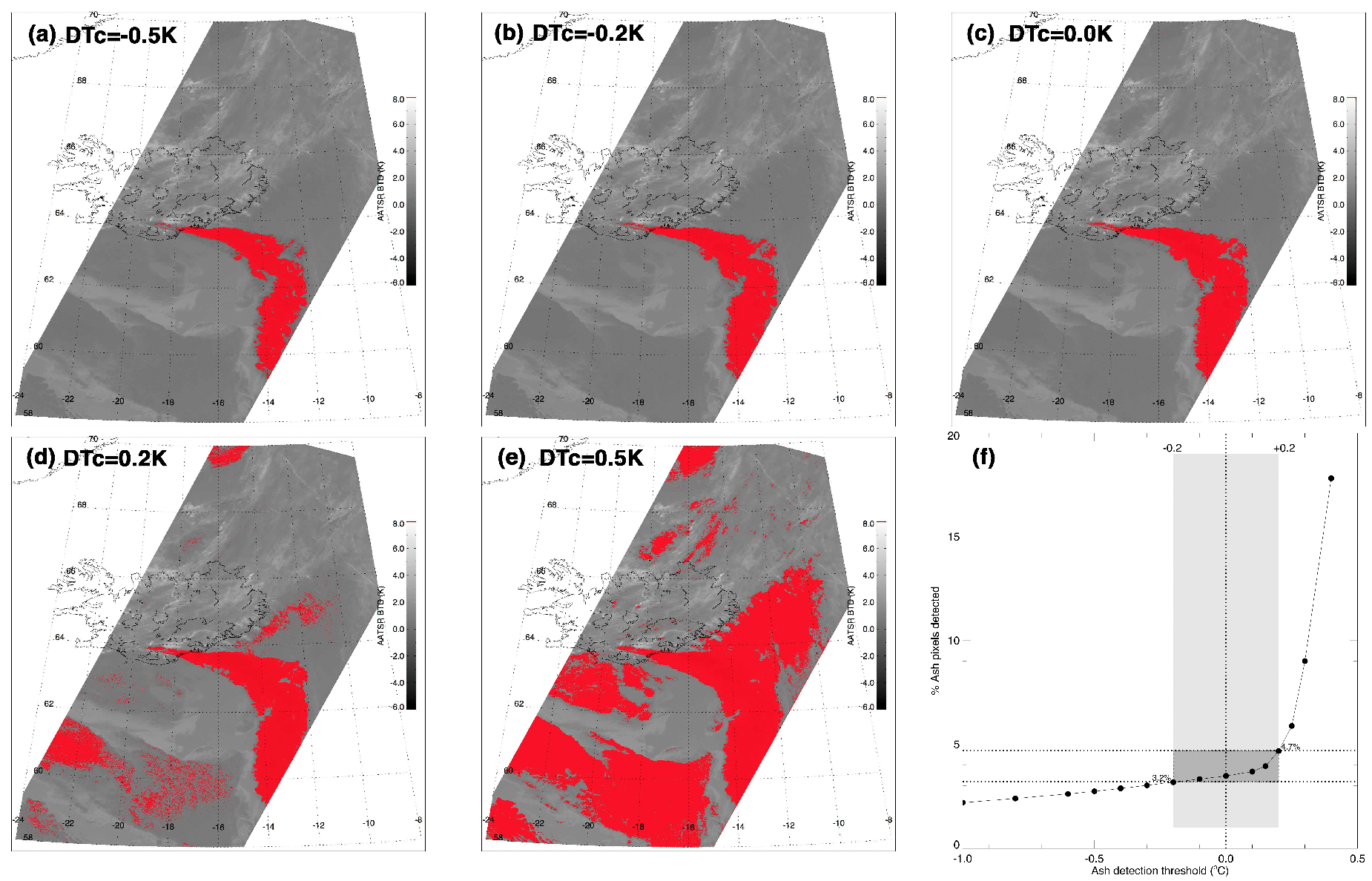
4.4. Setting the Detection Threshold
- The effect of water vapour absorption, which is highly variable, causes the BTD to increase so that it can be positive for ash affected pixels.
- Variable, spectral emissivity of the underlying surface can cause the BTD to be positive for ash affected pixels,
- Misalignment of the instantaneous fields of view (IFOVs) of the IR channels can cause the BTD to appear smaller or larger than expected, depending on the heterogeneity of the scene.
- Sub-pixel or mixed pixel effects can cause the BTD to appear smaller or larger than otherwise expected, depending on the scene heterogeneity.
4.5. Using More Than Two Channels
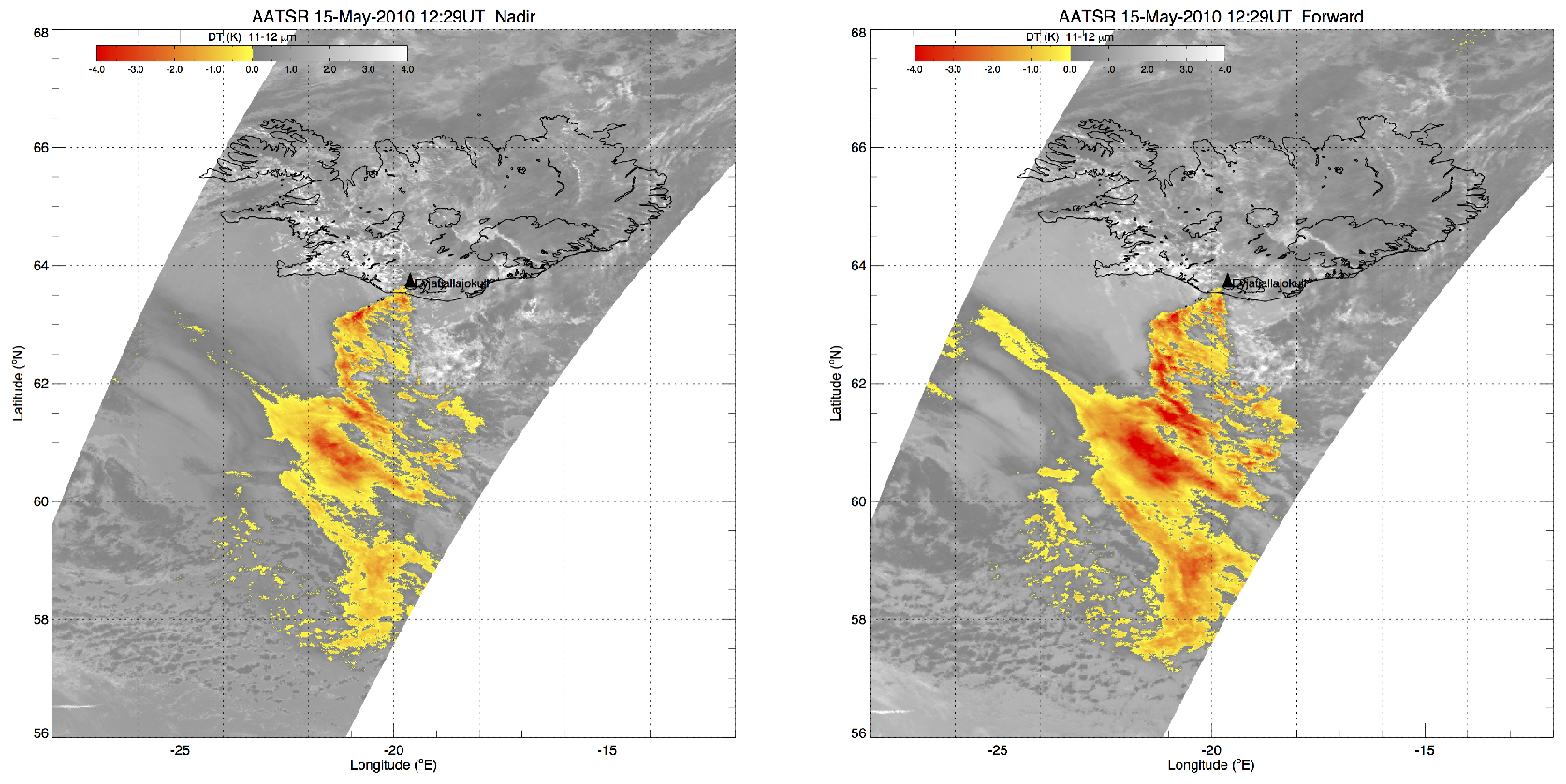
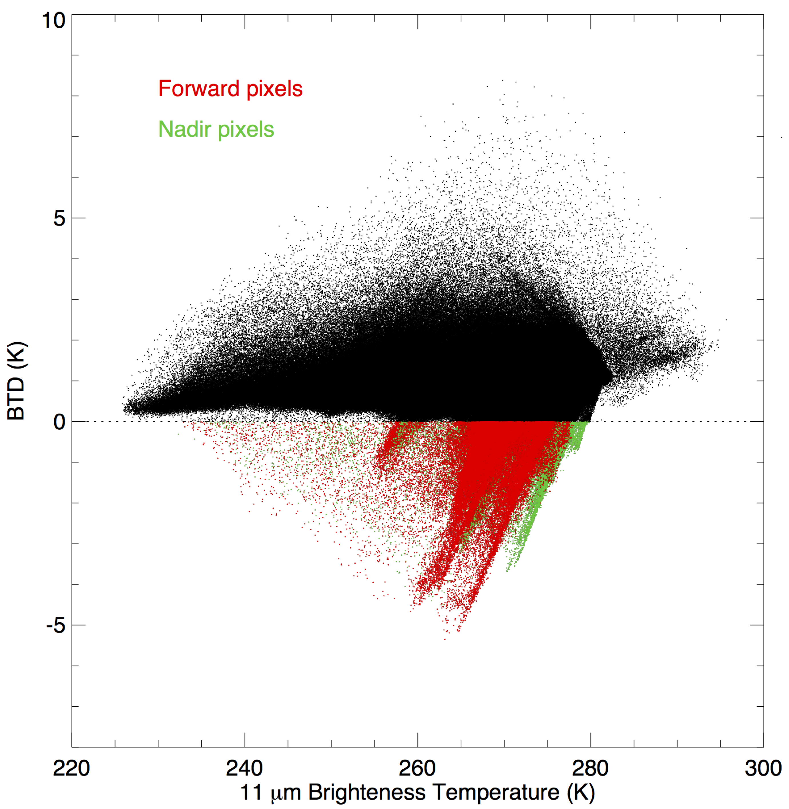
4.6. Exploiting Angular Dependence
5. Cloud Identification Scheme (CID)
5.1. Zenith Angle Effects
5.2. Land Surface Effects
5.3. Cloud Effects
- Low cloud uniformity test over the ocean.
- Clouds at moderate to high zenith angles.
- General cloud test.
- Cloud/SO test.
5.4. Water Vapour
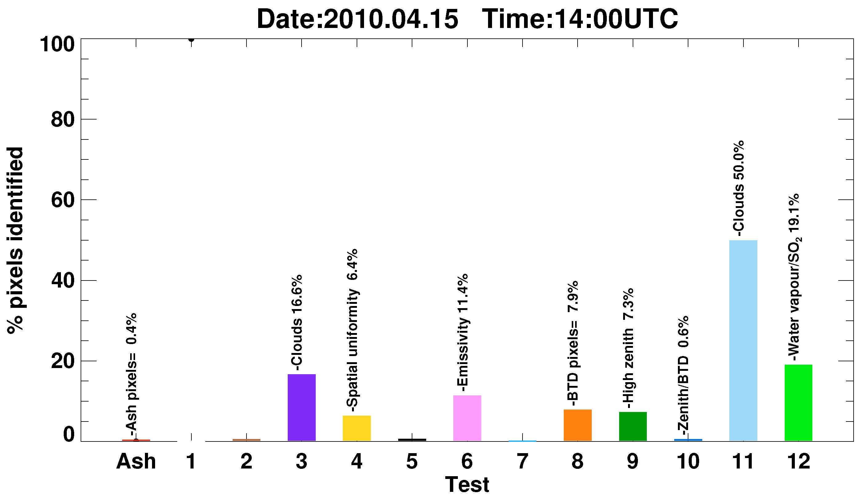
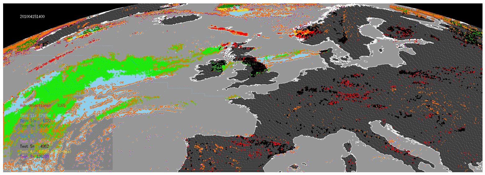
5.5. Summary and Example of the New Tests
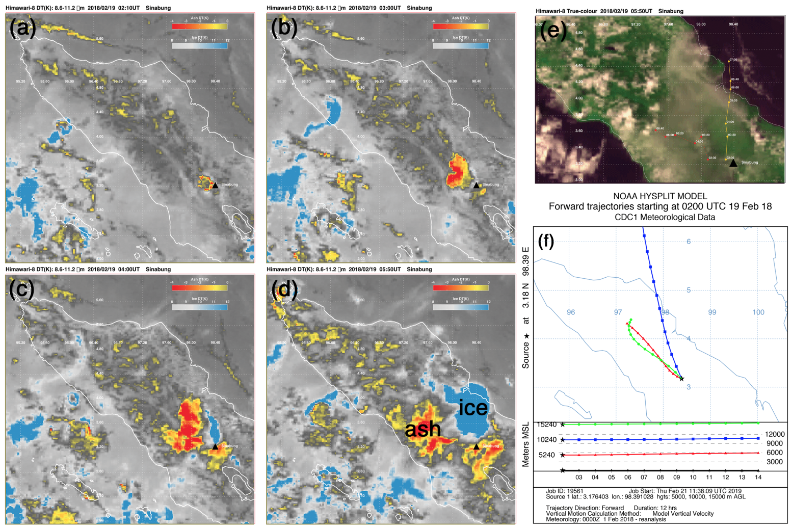
6. Volcanic Ice
6.1. Case study: Sinabung, Indonesia, 19 February 2018
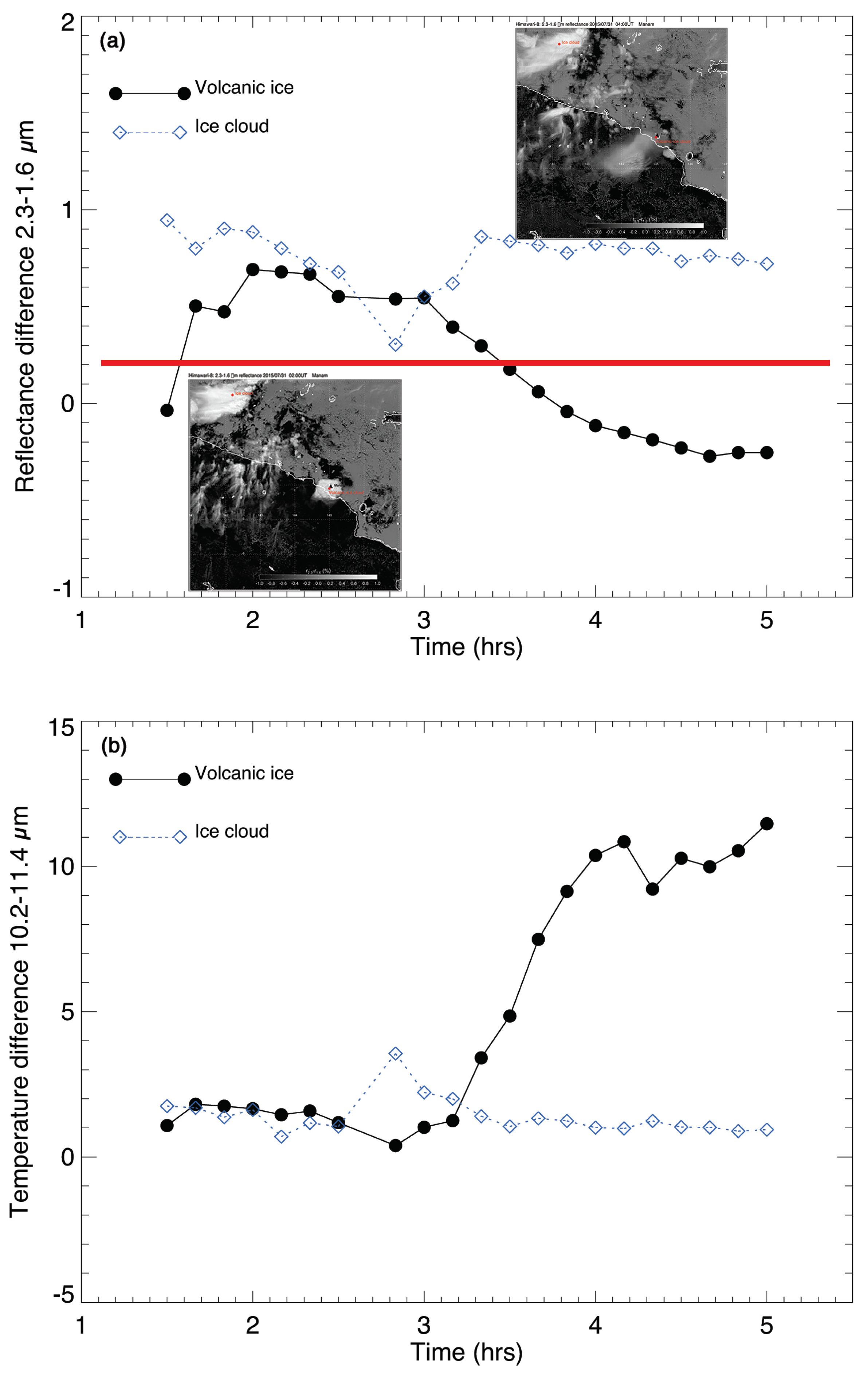
6.2. Case Study: Manam, PNG, 31 July 2015
7. Global Volcanic Emission Maps
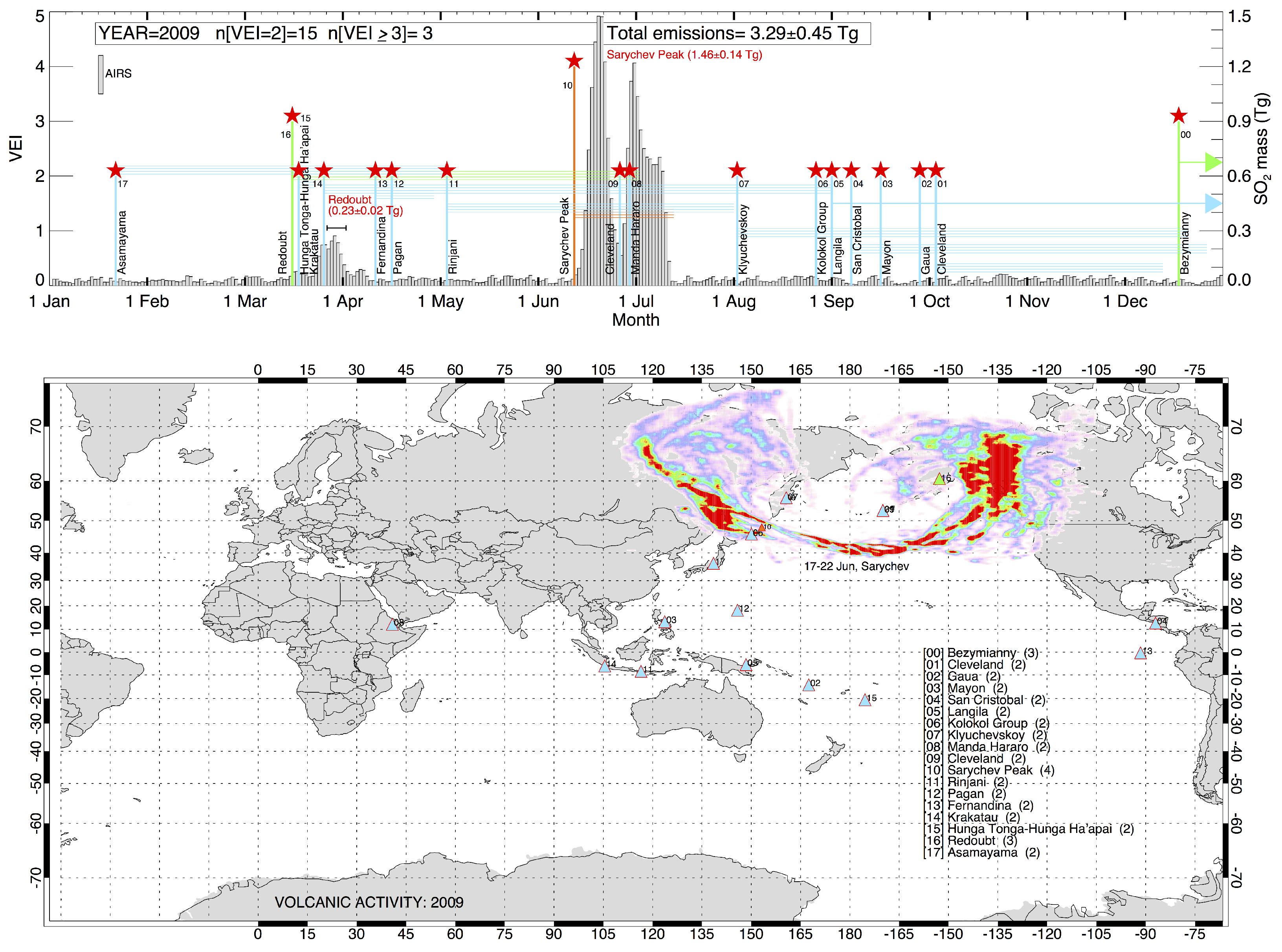
7.1. Annual Global Maps
7.2. Regional Maps
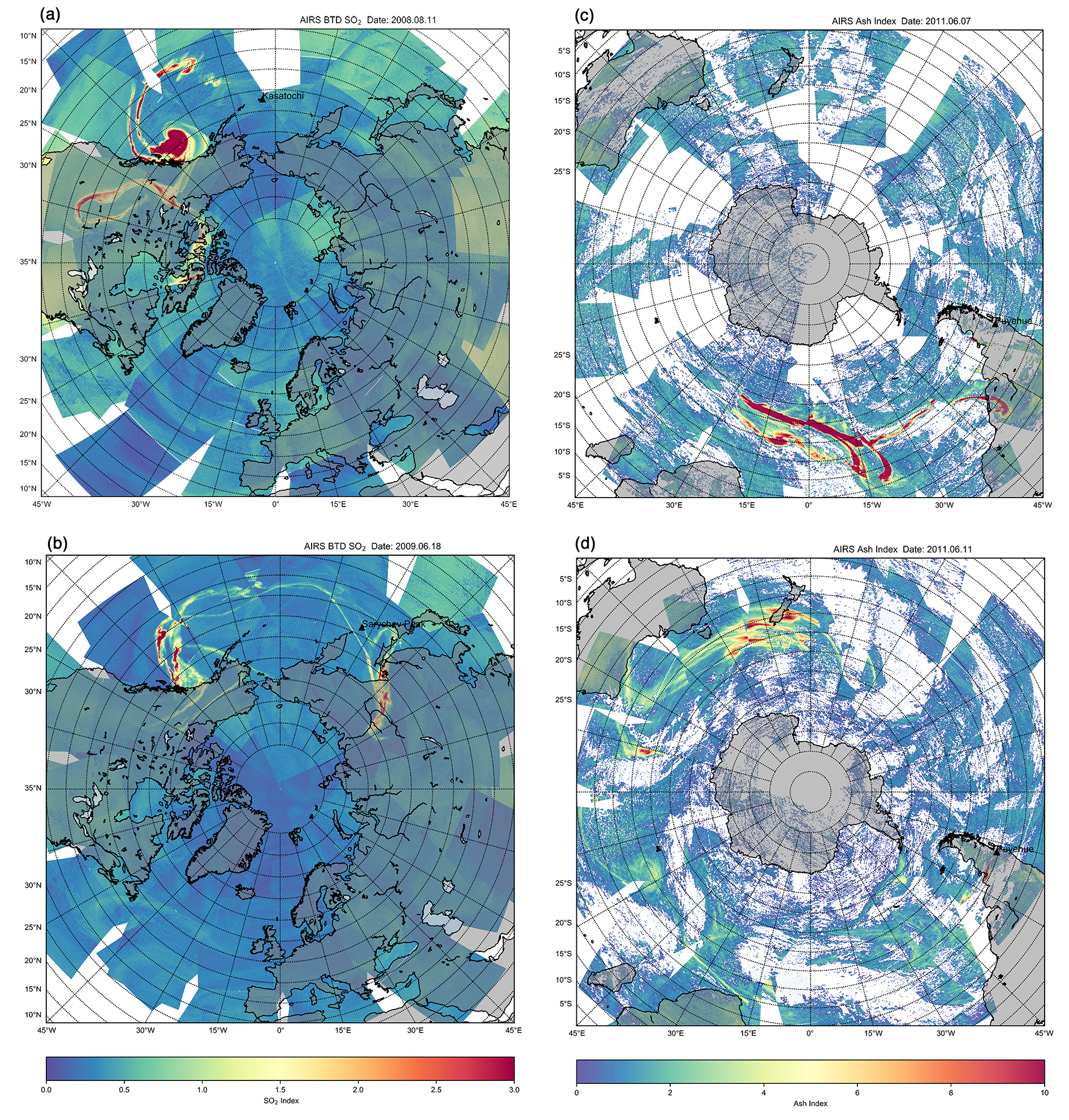
7.3. Hemispheric Daily Maps
8. Conclusions
Author Contributions
Funding
Acknowledgments
Conflicts of Interest
References
- Durant, A.J.; Bonadonna, C.; Horwell, C. Atmospheric and environmental impacts of volcanic particulates. Elements 2010, 6, 235–240. [Google Scholar] [CrossRef]
- Robock, A. Volcanic eruptions and climate. Rev. Geophys. 2000, 38, 191–219. [Google Scholar] [CrossRef] [Green Version]
- Casadevall, T.J. Volcanic Ash and Aviation Safety: Proceedings of the First International Symposium on Volcanic Ash and Aviation Safety; DIANE Publishing: Collingdale, PA, USA, 1994; Volume 2047. [Google Scholar]
- Prata, A.; Tupper, A. Aviation hazards from volcanoes: The state of the science. Nat. Hazards 2009, 51, 239–244. [Google Scholar] [CrossRef]
- Kramer, H.J. Observation of the Earth and Its Environment: Survey of Missions and Sensors; Springer Science & Business Media: Berlin, Germany, 2002. [Google Scholar]
- Marshak, A.; Herman, J.; Adam, S.; Karin, B.; Carn, S.; Cede, A.; Geogdzhayev, I.; Huang, D.; Huang, L.K.; Knyazikhin, Y.; et al. Earth Observations from DSCOVR EPIC Instrument. Bull. Am. Meteorol. Soc. 2018, 99, 1829–1850. [Google Scholar] [CrossRef] [Green Version]
- Carn, S.; Krotkov, N.; Fisher, B.; Li, C.; Prata, A. First Observations of Volcanic Eruption Clouds From the L1 Earth-Sun Lagrange Point by DSCOVR/EPIC. Geophys. Res. Lett. 2018, 45, 11–456. [Google Scholar] [CrossRef]
- Prata, A.T.; Young, S.A.; Siems, S.T.; Manton, M.J. Lidar ratios of stratospheric volcanic ash and sulfate aerosols retrieved from CALIOP measurements. Atmos. Chem. Phys. 2017, 17, 8599–8618. [Google Scholar] [CrossRef] [Green Version]
- Marzano, F.S.; Barbieri, S.; Vulpiani, G.; Rose, W.I. Volcanic ash cloud retrieval by ground-based microwave weather radar. IEEE Trans. Geosci. Remote Sens. 2006, 44, 3235–3246. [Google Scholar] [CrossRef]
- Montopoli, M.; Cimini, D.; Lamantea, M.; Herzog, M.; Graf, H.F.; Marzano, F.S. Microwave radiometric remote sensing of volcanic ash clouds from space: Model and data analysis. IEEE Trans. Geosci. Remote Sens. 2013, 51, 4678–4691. [Google Scholar] [CrossRef]
- Harris, A.J.; Flynn, L.P.; Dean, K.; Pilger, E.; Wooster, M.; Okubo, C.; Mouginis-Mark, P.; Garbeil, H.; Thornber, C.; De La Cruz-Reyna, S.; et al. Real-time satellite monitoring of volcanic hot spots. Remote Sens. Act. Volcanism 2000, 116, 139–159. [Google Scholar]
- Wright, R.; Flynn, L.P.; Garbeil, H.; Harris, A.J.; Pilger, E. MODVOLC: Near-real-time thermal monitoring of global volcanism. J. Volcanol. Geotherm. Res. 2004, 135, 29–49. [Google Scholar] [CrossRef]
- Bluth, G.J.; Doiron, S.D.; Schnetzler, C.C.; Krueger, A.J.; Walter, L.S. Global tracking of the SO2 clouds from the June, 1991 Mount Pinatubo eruptions. Geophys. Res. Lett. 1992, 19, 151–154. [Google Scholar] [CrossRef]
- Carn, S.; Krueger, A.J.; Krotkov, N.A.; Yang, K.; Evans, K. Tracking volcanic sulfur dioxide clouds for aviation hazard mitigation. Nat. Hazards 2009, 51, 325–343. [Google Scholar] [CrossRef]
- Thomas, W.; Erbertseder, T.; Ruppert, T.; Van Roozendael, M.; Verdebout, J.; Balis, D.; Meleti, C.; Zerefos, C. On the retrieval of volcanic sulfur dioxide emissions from GOME backscatter measurements. J. Atmos. Chem. 2005, 50, 295–320. [Google Scholar] [CrossRef]
- Khokhar, M.; Frankenberg, C.; Van Roozendael, M.; Beirle, S.; Kühl, S.; Richter, A.; Platt, U.; Wagner, T. Satellite observations of atmospheric SO2 from volcanic eruptions during the time-period of 1996–2002. Adv. Space Res. 2005, 36, 879–887. [Google Scholar] [CrossRef]
- Carn, S.; Yang, K.; Prata, A.; Krotkov, N. Extending the long-term record of volcanic SO2 emissions with the Ozone Mapping and Profiler Suite nadir mapper. Geophys. Res. Lett. 2015, 42, 925–932. [Google Scholar] [CrossRef]
- Theys, N.; Hedelt, P.; De Smedt, I.; Lerot, C.; Yu, H.; Vlietinck, J.; Pedergnana, M.; Arellano, S.; Galle, B.; Fernandez, D.; et al. Global monitoring of volcanic SO2 degassing with unprecedented resolution from TROPOMI onboard Sentinel-5 Precursor. Sci. Rep. 2019, 9, 2643. [Google Scholar] [CrossRef] [PubMed]
- Casadevall, T.; Delos Reyes, P.; Schneider, D. The 1991 Pinatubo eruptions and their effects on aircraft operations. In Fire and Mud: Eruptions and Lahars of Mount Pinatubo, Philippines; Newhall, C., Punongbayan, R., Eds.; Philippines Institute of Volcanology and Seismology: Quezon City, Philippines; University of Washington Press: Seattle, WA, USA, 1996; pp. 625–636. [Google Scholar]
- Miller, T.; Casadevall, T. Volcanic ash hazards to aviation. In Encyclopedia of Volcanoes; Sigurdsson, H., Houghton, B., McNutt, S.R., Ryman, H., Stix, J., Eds.; Academic Press: San Diego, CA, USA, 1999; pp. 915–930. [Google Scholar]
- Hanstrum, B.; Watson, A. A case study of two eruptions of Mount Galunggung and an investigation of volcanic cloud characteristics using remote sensing techniques. Aust. Meteorol. Mag. 1983, 31, 171–177. [Google Scholar]
- Prata, A. Infrared radiative transfer calculations for volcanic ash clouds. Geophys. Res. Lett. 1989, 16, 1293–1296. [Google Scholar] [CrossRef]
- Prata, A. Observations of volcanic ash clouds in the 10–12 μm window using AVHRR/2 data. Int. J. Remote Sens. 1989, 10, 751–761. [Google Scholar] [CrossRef]
- Barton, I.; Prata, A.; Watterson, I.; Young, S. Identification of the Mount Hudson volcanic cloud over SE Australia. Geophys. Res. Lett. 1992, 19, 1211–1214. [Google Scholar] [CrossRef]
- Ellrod, G.P.; Connell, B.H.; Hillger, D.W. Improved detection of airborne volcanic ash using multispectral infrared satellite data. J. Geophys. Res. Atmos. 2003, 108. [Google Scholar] [CrossRef] [Green Version]
- Rodgers, C.D. Inverse Methods for Atmospheric Sounding: Theory and Practice; World Scientific: Singapore, 2000; Volume 2. [Google Scholar]
- Twomey, S. Introduction to the Mathematics of Inversion in Remote Sensing and Indirect Measurements; Elsevier: Amsterdam, The Netherlands, 2013; Volume 3. [Google Scholar]
- Francis, P.N.; Cooke, M.C.; Saunders, R.W. Retrieval of physical properties of volcanic ash using Meteosat: A case study from the 2010 Eyjafjallajökull eruption. J. Geophys. Res. 2012, 117. [Google Scholar] [CrossRef] [Green Version]
- Pavolonis, M.J.; Heidinger, A.K.; Sieglaff, J. Automated retrievals of volcanic ash and dust cloud. J. Geophys. Res. Atmos. 2013, 118, 1436–1458. [Google Scholar] [CrossRef]
- Carboni, E.; Grainger, R.; Mather, T.A.; Pyle, D.M.; Dudhia, A.; Thomas, G.; Siddans, R.; Smith, A.; Koukouli, M.; Balis, D. The vertical distribution of volcanic SO2 plumes measured by IASI. Atmos. Chem. Phys. 2016, 16, 4343–4367. [Google Scholar] [CrossRef] [Green Version]
- Prata, A.; Grant, I. Retrieval of microphysical and morphological properties of volcanic ash plumes from satellite data: Application to Mt Ruapehu, New Zealand. Q. J. R. Meteorol. Soc. 2001, 127, 2153–2179. [Google Scholar] [CrossRef]
- Yu, T.; Rose, W.; Prata, A. Atmospheric correction for satellite-based volcanic ash mapping and retrievals using split window IR data from GOES and AVHRR. J. Geophys. Res. 2002, 107, AAC 10-1–AAC 10-19. [Google Scholar] [CrossRef]
- Prata, A.; Prata, A. Eyjafjallajökull volcanic ash concentrations determined using Spin Enhanced Visible and Infrared Imager measurements. J. Geophys. Res. 2012, 117. [Google Scholar] [CrossRef] [Green Version]
- Wen, S.; Rose, W.I. Retrieval of sizes and total masses of particles in volcanic clouds using AVHRR bands 4 and 5. J. Geophys. Res. 1994, 99, 5421–5431. [Google Scholar] [CrossRef]
- Watson, I.; Realmuto, V.; Rose, W.; Prata, A.; Bluth, G.; Gu, Y.; Bader, C.; Yu, T. Thermal infrared remote sensing of volcanic emissions using the moderate resolution imaging spectroradiometer. J. Volcanol. Geotherm. Res. 2004, 135, 75–89. [Google Scholar] [CrossRef]
- Grainger, R.; Peters, D.; Thomas, G.; Smith, A.; Siddans, R.; Carboni, E.; Dudhia, A. Measuring Volcanic Plume and Ash Properties from Space. In Remote-sensing of Volcanoes and Volcanic Processes: Integrating Observation and Modelling; Pyle, D.M., Mather, T.A., Biggs, J., Eds.; The Geological Society Special Publication: London, UK, 2013; Volume 380. [Google Scholar]
- Pavolonis, M.J.; Feltz, W.F.; Heidinger, A.K.; Gallina, G.M. A daytime complement to the reverse absorption technique for improved automated detection of volcanic ash. J. Atmos. Ocean. Technol. 2006, 23, 1422–1444. [Google Scholar] [CrossRef]
- Griessbach, S.; Hoffmann, L.; Höpfner, M.; Riese, M.; Spang, R. Scattering in infrared radiative transfer: A comparison between the spectrally averaging model JURASSIC and the line-by-line model KOPRA. J. Quant. Spectrosc. Radiat. Transf. 2013, 127, 102–118. [Google Scholar] [CrossRef]
- Griessbach, S.; Hoffmann, L.; Spang, R.; Riese, M. Volcanic ash detection with infrared limb sounding: MIPAS observations and radiative transfer simulations. Atmos. Meas. Tech. 2014, 7, 1487–1507. [Google Scholar] [CrossRef] [Green Version]
- Prata, G.; Ventress, L.; Carboni, E.; Mather, T.; Grainger, R.; Pyle, D. A new parameterization of volcanic ash complex refractive index based on NBO/T and SiO2 content. J. Geophys. Res. Atmos. 2018, 124, 1779–1797. [Google Scholar] [CrossRef]
- Heintzenberg, J. Properties of the log-normal particle size distribution. Aerosol Sci. Technol. 1994, 21, 46–48. [Google Scholar] [CrossRef]
- Farlow, N.H.; Oberbeck, V.R.; Snetsinger, K.G.; Ferry, G.V.; Polkowski, G.; Hayes, D.M. Size distributions and mineralogy of ash particles in the stratosphere from eruptions of Mount St. Helens. Science 1981, 211, 832–834. [Google Scholar] [CrossRef]
- Ventress, L.J.; McGarragh, G.; Carboni, E.; Smith, A.J.; Grainger, R.G. Retrieval of ash properties from IASI measurements. Atmos. Meas. Tech. 2016, 9, 5407–5422. [Google Scholar] [CrossRef] [Green Version]
- Clarisse, L.; Prata, F. Infrared sounding of volcanic ash. In Volcanic Ash; Elsevier: Amsterdam, The Netherlands, 2016; pp. 189–215. [Google Scholar]
- Pergola, N.; Tramutoli, V.; Marchese, F.; Scaffidi, I.; Lacava, T. Improving volcanic ash cloud detection by a robust satellite technique. Remote Sens. Environ. 2004, 90, 1–22. [Google Scholar] [CrossRef]
- Prata, A.F.; Cechet, R.P.; Barton, I.J.; Llewellyn-Jones, D.T. The along track scanning radiometer for ERS-1-scan geometry and data simulation. IEEE Trans. Geosci. Remote Sens. 1990, 28, 3–13. [Google Scholar] [CrossRef]
- Prata, A.J.; Turner, P. Cloud-top height determination using ATSR data. Remote Sens. Environ. 1997, 59, 1–13. [Google Scholar] [CrossRef]
- Muller, J.P.; Denis, M.A.; Dundas, R.D.; Mitchell, K.L.; Naud, C.; Mannstein, H. Stereo cloud-top heights and cloud fraction retrieval from ATSR-2. Int. J. Remote Sens. 2007, 28, 1921–1938. [Google Scholar] [CrossRef]
- Saunders, R.W.; Kriebel, K.T. An improved method for detecting clear sky and cloudy radiances from AVHRR data. Int. J. Remote Sens. 1988, 9, 123–150. [Google Scholar] [CrossRef] [Green Version]
- Mosher, F.R. Four channel volcanic ash detection algorithm. In Proceedings of the 10th Conference on Satellite Meteorology and Oceanography, Long Beach, CA, USA, 9–14 January 2000; pp. 457–460. [Google Scholar]
- Ellrod, G.P. Impact on volcanic ash detection caused by the loss of the 12.0 μm Split Window band on GOES Imagers. J. Volcanol. Geotherm. Res. 2004, 135, 91–103. [Google Scholar] [CrossRef]
- Pavolonis, M.J.; Heidinger, A.K. Daytime cloud overlap detection from AVHRR and VIIRS. J. Appl. Meteorol. 2004, 43, 762–778. [Google Scholar] [CrossRef]
- Pavolonis, M.J.; Heidinger, A.K.; Uttal, T. Daytime global cloud typing from AVHRR and VIIRS: Algorithm description, validation, and comparisons. J. Appl. Meteorol. 2005, 44, 804–826. [Google Scholar] [CrossRef]
- Lee, K.H.; Wong, M.S.; Chung, S.R.; Sohn, E. Improved volcanic ash detection based on a hybrid reverse absorption technique. Atmos. Res. 2014, 143, 31–42. [Google Scholar] [CrossRef]
- Prata, A.J.; Bluth, G.; Rose, B.; Schneider, D.; Tupper, A. Comments on Failures in detecting volcanic ash from a satellite-based technique. Remote Sens. Environ. 2001, 78, 341–346. [Google Scholar] [CrossRef]
- Sobrino, J.; Coll, C.; Caselles, V. Atmospheric correction for land surface temperature using NOAA-11 AVHRR channels 4 and 5. Remote Sens. Environ. 1991, 38, 19–34. [Google Scholar] [CrossRef]
- Prata, A.J. Land surface temperatures derived from the advanced very high resolution radiometer and the along-track scanning radiometer: 1. Theory. J. Geophys. Res. Atmos. 1993, 98, 16689–16702. [Google Scholar] [CrossRef]
- Hulley, G.C.; Hook, S.J. Intercomparison of versions 4, 4.1 and 5 of the MODIS Land Surface Temperature and Emissivity products and validation with laboratory measurements of sand samples from the Namib desert, Namibia. Remote Sens. Environ. 2009, 113, 1313–1318. [Google Scholar] [CrossRef]
- Li, Z.L.; Tang, B.H.; Wu, H.; Ren, H.; Yan, G.; Wan, Z.; Trigo, I.F.; Sobrino, J.A. Satellite-derived land surface temperature: Current status and perspectives. Remote Sens. Environ. 2013, 131, 14–37. [Google Scholar] [CrossRef] [Green Version]
- Prata, A.J. Land surface temperatures derived from the advanced very high resolution radiometer and the along-track scanning radiometer: 2. Experimental results and validation of AVHRR algorithms. J. Geophys. Res. Atmos. 1994, 99, 13025–13058. [Google Scholar] [CrossRef]
- McAtee, B.; Prata, A.; Lynch, M. The Angular Behavior of Emitted Thermal Infrared Radiation (8–12 μm) at a Semiarid Site. J. Appl. Meteorol. 2003, 42, 1060–1071. [Google Scholar] [CrossRef]
- Rose, W.I.; Delene, D.; Schneider, D.; Bluth, G.; Krueger, A.; Sprod, I.; McKee, C.; Davies, H.; Ernst, G. Ice in the 1994 Rabaul eruption cloud: Implications for volcano hazard and atmospheric effects. Nature 1995, 375, 477–479. [Google Scholar] [CrossRef]
- Tupper, A.; Itikarai, I.; Richards, M.; Prata, F.; Carn, S.; Rosenfeld, D. Facing the challenges of the international airways volcano watch: The 2004/05 eruptions of Manam, Papua New Guinea. Weather Forecast. 2007, 22, 175–191. [Google Scholar] [CrossRef]
- Durant, A.; Shaw, R.; Rose, W.; Mi, Y.; Ernst, G. Ice nucleation and overseeding of ice in volcanic clouds. J. Geophys. Res. 2008, 113. [Google Scholar] [CrossRef] [Green Version]
- Hoyle, C.; Pinti, V.; Welti, A.; Zobrist, B.; Marcolli, C.; Luo, B.; Höskuldsson, Á.; Mattsson, H.; Stetzer, O.; Thorsteinsson, T.; et al. Ice nucleation properties of volcanic ash from Eyjafjallajökull. Atmos. Chem. Phys. 2011, 11, 9911–9926. [Google Scholar] [CrossRef] [Green Version]
- Durant, A.J.; Shaw, R.A. Evaporation freezing by contact nucleation inside-out. Geophys. Res. Lett. 2005, 32. [Google Scholar] [CrossRef] [Green Version]
- Bingemer, H.; Klein, H.; Ebert, M.; Haunold, W.; Bundke, U.; Herrmann, T.; Kandler, K.; Müller-Ebert, D.; Weinbruch, S.; Judt, A.; et al. Atmospheric ice nuclei in the Eyjafjallajökull volcanic ash plume. Atmos. Chem. Phys. 2012, 12, 857–867. [Google Scholar] [CrossRef] [Green Version]
- Mangan, T.; Atkinson, J.; Neuberg, J.; O’Sullivan, D.; Wilson, T.; Whale, T.; Neve, L.; Umo, N.; Malkin, T.; Murray, B. Heterogeneous ice nucleation by soufriere hills volcanic ash immersed in water droplets. PLoS ONE 2017, 12, e0169720. [Google Scholar] [CrossRef]
- Atkinson, J.D.; Murray, B.J.; Woodhouse, M.T.; Whale, T.F.; Baustian, K.J.; Carslaw, K.S.; Dobbie, S.; O’Sullivan, D.; Malkin, T.L. The importance of feldspar for ice nucleation by mineral dust in mixed-phase clouds. Nature 2013, 498, 355–358. [Google Scholar] [CrossRef] [PubMed] [Green Version]
- Genareau, K.; Cloer, S.; Primm, K.; Tolbert, M.; Woods, T. Compositional and Mineralogical Effects on Ice Nucleation Activity of Volcanic Ash. Atmosphere 2018, 9, 238. [Google Scholar] [CrossRef]
- Prata, F.; Woodhouse, M.; Huppert, H.E.; Prata, A.; Thordarson, T.; Carn, S. Atmospheric processes affecting the separation of volcanic ash and SO2 in volcanic eruptions: Inferences from the May 2011 Grímsvötn eruption. Atmos. Chem. Phys. 2017, 17, 10709–10732. [Google Scholar] [CrossRef]
- Dampier, W. A Voyage to New Holland; Nonsuch Publishing Limited: Stroud, UK, 2006; p. 222. [Google Scholar]
- Sennert, S.K.E. Weekly Volcanic Activity Report, 29 July–4 August 2015; Global Volcanism Program: Washington, DC, USA, 2015. [Google Scholar]
- Platnick, S.; King, M.D.; Meyer, K.G.; Wind, G.; Amarasinghe, N.; Marchant, B.; Arnold, G.T.; Zhang, Z.; Hubanks, P.A.; Ridgway, B.; et al. MODIS cloud optical properties: User guide for the Collection 6 Level-2 MOD06/MYD06 product and associated Level-3 Datasets. Version 2015, 1, 145. [Google Scholar]
- Herzog, M.; Graf, H.F. Applying the three-dimensional model ATHAM to volcanic plumes: Dynamic of large co-ignimbrite eruptions and associated injection heights for volcanic gases. Geophys. Res. Lett. 2010, 37. [Google Scholar] [CrossRef] [Green Version]
- Suzuki, Y.; Koyaguchi, T. A three-dimensional numerical simulation of spreading umbrella clouds. J. Geophys. Res. Solid Earth 2009, 114. [Google Scholar] [CrossRef] [Green Version]
- Marti, A.; Folch, A.; Jorba, O.; Janjic, Z. Volcanic ash modeling with the online NMMB-MONARCH-ASH v1. 0 model: Model description, case simulation, and evaluation. Atmos. Chem. Phys. 2017, 17, 4005–4030. [Google Scholar] [CrossRef]
- Wu, X.; Griessbach, S.; Hoffmann, L. Equatorward dispersion of a high-latitude volcanic plume and its relation to the Asian summer monsoon: A case study of the Sarychev eruption in 2009. Atmos. Chem. Phys. 2017, 17, 13439. [Google Scholar] [CrossRef]
- Prata, A.; Bernardo, C. Retrieval of volcanic SO2 column abundance from Atmospheric Infrared Sounder data. J. Geophys. Res. 2007, 112. [Google Scholar] [CrossRef]
- Newhall, C.G.; Self, S. The volcanic explosivity index (VEI) an estimate of explosive magnitude for historical volcanism. J. Geophys. Res. Oceans 1982, 87, 1231–1238. [Google Scholar] [CrossRef]
- Thomas, H.; Prata, A. Computer vision for improved estimates of SO2 emission rates and plume dynamics. Int. J. Remote Sens. 2018, 39, 1285–1305. [Google Scholar] [CrossRef]
- Kremser, S.; Thomason, L.W.; von Hobe, M.; Hermann, M.; Deshler, T.; Timmreck, C.; Toohey, M.; Stenke, A.; Schwarz, J.P.; Weigel, R.; et al. Stratospheric aerosol–Observations, processes, and impact on climate. Rev. Geophys. 2016, 54, 278–335. [Google Scholar] [CrossRef]
- Thomas, H.E.; Prata, A.J. Sulphur dioxide as a volcanic ash proxy during the April and May 2010 eruption of Eyjafjallajökull Volcano, Iceland. Atmos. Chem. Phys. 2011, 11, 6871–6880. [Google Scholar] [CrossRef]
- Mastin, L.; Guffanti, M.; Servranckx, R.; Webley, P.; Barsotti, S.; Dean, K.; Durant, A.; Ewert, J.; Neri, A.; Rose, W.; et al. A multidisciplinary effort to assign realistic source parameters to models of volcanic ash-cloud transport and dispersion during eruptions. J. Volcanol. Geotherm. Res. 2009, 186, 10–21. [Google Scholar] [CrossRef] [Green Version]
- Prata, A.; Rose, W.; Self, S.; O’Brien, D. Global, long-term sulphur dioxide measurements from TOVS data: A new tool for studying explosive volcanism and climate. Volcanism Earth’s Atmos. 2003, 139, 75–92. [Google Scholar] [CrossRef]
- Carn, S.; Clarisse, L.; Prata, A. Multi-decadal satellite measurements of global volcanic degassing. J. Volcanol. Geotherm. Res. 2016, 311, 99–134. [Google Scholar] [CrossRef] [Green Version]
- Prata, A.; Dezitter, F.; Davies, I.; Weber, K.; Birnfeld, M.; Moriano, D.; Bernardo, C.; Vogel, A.; Prata, G.S.; Mather, T.A.; et al. Artificial cloud test confirms volcanic ash detection using infrared spectral imaging. Sci. Rep. 2016, 6, 25620. [Google Scholar] [CrossRef] [Green Version]
- Marzano, F.S.; Picciotti, E.; Montopoli, M.; Vulpiani, G. Inside Volcanic Clouds: Remote Sensing of Ash Plumes Using Microwave Weather Radars. Bull. Am. Meteorol. Soc. 2013, 94, 1567–1586. [Google Scholar] [CrossRef]
- Winker, D.; Liu, Z.; Omar, A.; Tackett, J.; Fairlie, D. CALIOP observations of the transport of ash from the Eyjafjallajökull volcano in April 2010. J. Geophys. Res. Atmos. 2012, 117. [Google Scholar] [CrossRef] [Green Version]
- Sawada, Y. Study on Analyses of Volcanic Eruptions Based on Eruption Cloud Image Data Obtained by the Geostationary Meteorological Satellite (GMS); Technical Reports of the Meteorological Research Institute; Meteorological Research Institute: Ibaraki, Japan, 1987.
- Sawada, Y. Detection of explosive eruptions and regional tracking of volcanic ash clouds with Geostationary Meteorological Satellite (GMS). In Monitoring and Mitigation of Volcano Hazards; Springer: Berlin, Germany, 1996; pp. 299–314. [Google Scholar]
- Matson, M. The 1982 El Chichón volcano eruptions—A satellite perspective. J. Volcanol. Geotherm. Res. 1984, 23, 1–10. [Google Scholar] [CrossRef]
- Robock, A.; Matson, M. Circumglobal transport of the El Chichón volcanic dust cloud. Science 1983, 221, 195–197. [Google Scholar] [CrossRef]
- Malingreau, J.P.; Kaswanda. Monitoring volcanic eruptions in Indonesia using weather satellite data: The Colo eruption of July 28, 1983. J. Volcanol. Geotherm. Res. 1986, 27, 179–194. [Google Scholar] [CrossRef]
- Potts, R. Satellite observations of Mt Pinatubo ash clouds. Aust. Meteorol. Mag. 1993, 42, 59–68. [Google Scholar]
- Tupper, A.C.; Davey, J.P.; Potts, R.J. Monitoring volcanic eruptions in Indonesia and the Southwest Pacific. In Researching Eruption Clouds on Volcanic Island Chains; Kagoshima University Research Center for the Pacific Islands, Occasional Papers No. 2003; Kagoshima University: Kagoshima, Japan, 2003. [Google Scholar]
- Gupta, R.; Badarinath, K. Volcano monitoring using remote sensing data. Int. J. Remote Sens. 1993, 14, 2907–2918. [Google Scholar] [CrossRef]
- Oppenheimer, C.; Rothery, D. Infrared monitoring of volcanoes by satellite. J. Geol. Soc. 1991, 148, 563–569. [Google Scholar] [CrossRef]
- Dean, K.G.; Dehn, J. Monitoring Volcanoes in the North Pacific: Observations from Space; Springer Science & Business Media: Berlin, Germany, 2015. [Google Scholar]
- Papale, P. Volcanic Hazards, Risks and Disasters; Elsevier: Amsterdam, The Netherlands, 2015. [Google Scholar]
- Mackie, S.; Cashman, K.; Ricketts, H.; Rust, A.; Watson, M. Volcanic Ash: Hazard Observation; Elsevier: Amsterdam, The Netherlands, 2016. [Google Scholar]


| Satellite | Local Equatorial | Inclination | Height | Period | Repeat Cycle |
|---|---|---|---|---|---|
| Crossing Time | (Degrees) | (km) | (Minutes) | (Days) | |
| Landsat-5 | 09:45 | 98.2 | 704 | 99 | 16 |
| Landsat-7 | 10:00 | 98.2 | 705 | 99 | 16 |
| Landsat-8 | 10:30 | 98.2 | 701–703 | 98.8 | 16 |
| NOAA-11 | 13:40(A) | 98.9 | 845–863 | 102.1 | 11 |
| NOAA-12 | 19:30(A) | 98.7 | 806–825 | 101.3 | 11 |
| NOAA-13 | Failed 11 days after launch | ||||
| NOAA-14 | 13:40(A) | 98.9 | 848–861 | 102.1 | 11 |
| NOAA-15 | 16:44(A) | 98.7 | 804–818 | 101.3 | 11 |
| NOAA-16 | 14:00(A) | 98.74 | 845–860 | 102.1 | 11 |
| NOAA-17 | 22:00(A) | 98.52 | 800–817 | 101.1 | 11 |
| NOAA-18 | 14:00(A) | 99.1 | 840–862 | 102 | 11 |
| NOAA-19 | 13:34(A) | 99.1 | 840–862 | 102 | 11 |
| NPP | 13:30(A) | 98.74 | 824 | 101 | 16 |
| ERS-1 | 10:30(D) | 98.52 | 782–785 | 100 | 35 |
| ERS-2 | 10:30(A) | 98.5 | 780 | 100 | 35 |
| ENVISAT | 10:30(A) | 98.5 | 780 | 100 | 35 |
| Aqua | 13:30(A) | 98.2 | 705 | 98.8 | 16 |
| Terra | 10:30(D) | 98.5 | 705 | 99.0 | 16 |
| Aura | 13:45(A) | 98.7 | 705 | 98.8 | 16 |
| MetOP-A/B/C | 21:30 (A) | 98.7 | 817–827 | 101 | 29 |
| Sentinel-2A/2B | 10:30 | 98.62 | 786 | 100.6 | 10 |
| Sentinel-3A/3B | 10:00 | 98.65 | 814.5 | 100.99 | 27 |
| Sensor | Ash Bands μm | SO Bands μm | Resolution km | Platform pol or geo | Time Period Years |
|---|---|---|---|---|---|
| AVHRR-2/3 | 3.7, 10.8, 12.0 | – | 1 | p | 1979–present |
| HIRS-2/3 | 3.76–4.57, 11.11, 12.47 | 7.3, 8.2 | 26 × 42 | p | 1979-present |
| MODIS | 3.75–4.5, 8.6, 11.03, 12.03 | 7.33, 8.55 | 1 | p | 2000–present |
| SEVIRI | 3. 8.7, 10.8, 12.0 | 7.35, 8.7 | 2 | g (15) | 2004–present |
| IMAGER/MTSAT-2 | 3.75, 10.8, 12.0 | – | 4 | g (30) | 2006–05/2016 |
| AHI/HIMAWARI-8 | 3.85, 8.60, 10.4, 11.2, 12.4 | 7.35, 8.6 | 2 | g (10) | 2004–present |
| ABI | 3.9, 8.5, 10.2, 11.2, 12.3 | 8.5 | 2 | g (15) | 2017–present |
| AIRS | 3.74–4.61, 8.80–15.4 | 6.2–8.22 | 13.5 | p | 2002-present |
| IASI | 3.62–5.00, 8.26–15.50 | 5–8.26 | 12.0 | p | 2007–present |
| ASTER | 8.30, 8.65, 10.6, 11.3 | 8.30, 8.65 | 0.09 | p | 2000–present |
| ATSR/ATSR-2/AATSR | 3.7, 10.85, 12.0 | – | 1 | p | 1991–03/2000 |
| SLSTR | 3.74, 10.85, 12.0 | – | 1 | p | 07/2016–present |
| TM/Landsat-5 | 11.45 | – | 0.12 | p | 1984–06/2013 |
| ETM+/Landsat-7 | 11.45 | – | 0.06 | p | 1999–present |
| TM/Landsat-8 | 10.8, 12.0 | – | 0.1 | p | 1982-11/2011 |
| Volcano | |||||||
|---|---|---|---|---|---|---|---|
| Oxide | Rinjani | Agung | Cháiten | Eyjafjallajökull | Grímsvötn | Etna | Askja |
| SiO | 64.29 | 53.82 | 73.23 | 57.38 | 49.13 | 47.14 | 70.65 |
| TiO | 0.58 | 1.06 | 0.15 | 1.52 | 2.84 | 1.76 | 0.84 |
| AlO | 18.76 | 20.12 | 13.83 | 14.66 | 13.25 | 17.47 | 12.28 |
| FeO | 4.41 | 8.75 | 1.60 | 10.02 | 14.87 | 11.38 | 4.35 |
| FeO | 3.58 | 7.10 | – | – | – | – | – |
| MnO | 0.14 | 0.18 | 0.062 | 0.243 | 0.213 | 0.171 | 0.110 |
| MgO | 0.92 | 2.85 | 0.34 | 2.49 | 5.20 | 5.18 | 0.84 |
| CaO | 3.00 | 8.54 | 1.51 | 4.91 | 9.63 | 9.89 | 2.56 |
| NaO | 4.15 | 3.32 | 4.18 | 5.53 | 2.82 | 3.60 | 3.96 |
| KO | 3.55 | 1.12 | 2.957 | 1.928 | 0.468 | 2.048 | 2.317 |
| PO | 0.20 | 0.23 | 0.062 | 0.315 | 0.305 | 0.574 | 0.167 |
| SO | <0.003 | 0.013 | 0.377 | 0.056 | <0.003 | 0.155 | <0.003 |
| LOI | 5.26 | 2.43 | 1.33 | −0.17 | −0.42 | −0.09 | 1.02 |
| Total | 100.4 | 98.64 | 99.23 | 98.84 | 98.67 | 99.18 | 99.10 |
| Volcano | |||||||
|---|---|---|---|---|---|---|---|
| Oxide | Spurr | Redoubt | Sakurajima | Kelud | Merapi | Hudson | Copahue |
| SiO | 55.42 | 60.45 | 60.0 | 56.1 | 54.69 | 47.60 | 52.07 |
| TiO | 0.72 | 0.56 | 0.16 | 0.18 | 0.74 | 2.19 | 1.25 |
| AlO | 18.76 | 17.83 | 18.3 | 19.2 | 19.29 | 16.35 | 17.54 |
| FeO | 7.99 | 6.47 | – | – | – | 11.48 | 8.28 |
| FeO | – | – | 5.70 | 4.89 | 7.76 | – | – |
| MnO | 0.152 | 0.145 | 0.07 | 0.14 | 0.19 | 1.96 | 1.40 |
| MgO | 4.40 | 2.41 | 4.10 | 5.33 | 2.25 | 4.37 | 4.39 |
| CaO | 7.55 | 6.27 | 7.41 | 11.6 | 8.12 | 8.23 | 7.09 |
| NaO | 3.44 | 4.01 | 3.27 | 2.26 | 3.73 | 4.08 | 3.60 |
| KO | 0.953 | 1.462 | 0.76 | 0.41 | 2.16 | 1.27 | 1.86 |
| PO | 0.233 | 0.211 | – | – | 0.30 | 0.74 | 0.28 |
| SO | – | – | – | – | 0.03 | – | – |
| LOI | 0.51 | 0.29 | – | – | – | −0.31 | 1.15 |
| Total | 100.30 | 100.12 | 99.70 | 100 | 99.28 | 97.95 | 98.91 |
| Parameter | ATSR | ATSR-2 | AATSR | SLSTR |
|---|---|---|---|---|
| Channel (width), m | ||||
| 0.55 (0.02) | • | • | • | • |
| 0.67 (0.02) | • | • | • | • |
| 0.87 (0.02) | • | • | • | • |
| 1.38 (0.015) | – | – | – | • |
| 1.61 (0.06) | – | • | • | • |
| 2.25 (0.05) | – | – | – | • |
| 3.70 (0.38) | • | • | • | • |
| 10.9 (0.9) | • | • | • | • |
| 12.0 (1.0) | • | • | • | • |
| Nadir swath width (km) | 505 | 505 | 505 | 740 |
| Forward swath width (km) | 512 | 512 | 512 | 1420 |
| Nadir angle (centre) (°) | 0 | 0 | 0 | 0 |
| Forward angle (centre (°) | 55 | 55 | 55 | 55 |
| Spatial resolution (km)—SWIR/visible | 1 | 1 | 1 | 0.5 |
| Spatial resolution (km)—Thermal IR | 1 | 1 | 1 | 1 |
| NET @ 300 K (mK) (thermal) | <500 | <500 | <500 | <500 |
| Operational dates | 7/1991–3/2000 | 4/1995–9/2011 | 3/2002–5/2012 | 2/2016–present (S3A) |
| 4/2018–present (S3B) |
| Test | Algorithm | Criteria | Description |
|---|---|---|---|
| 0 | =–0.8 K | BTD, reverse absorption Prata (1989b) | |
| 1 | = 0.0 K | Cloud test | |
| 2 | /cos() | = −0.2 K | Zenith angle () dependent BTD |
| 3 | > | N = 5 and = −0.9 K (ocean) −0.3 K (land) | Spatial uniformity test |
| 4 | > +(t) and < | = −0.2; = 250 K | Emissivity test over land |
| >; (t) = −1 + cos(2 t/24) | = 0.988, = 0.970; t = time in hours | ||
| 5 | > and < | = 240 K | Low uniform cloud over ocean |
| 6 | < and > cos() | = 200 K | Clouds at high zenith angles at night |
| 7 | < and > | = −0.5 K | SO/Ash test. Not used currently |
| 8 | < and > | = 75° | Excludes pixels beyond zenith angle |
| 9 | > and > | = 7 K; = 72° | High zenith cloud test |
| 10 | < | = −5 K | Cloud/SO test over the ocean |
| 11 | > | = 20 K | Water vapour/high altitude SO test |
© 2019 by the authors. Licensee MDPI, Basel, Switzerland. This article is an open access article distributed under the terms and conditions of the Creative Commons Attribution (CC BY) license (http://creativecommons.org/licenses/by/4.0/).
Share and Cite
Prata, F.; Lynch, M. Passive Earth Observations of Volcanic Clouds in the Atmosphere. Atmosphere 2019, 10, 199. https://doi.org/10.3390/atmos10040199
Prata F, Lynch M. Passive Earth Observations of Volcanic Clouds in the Atmosphere. Atmosphere. 2019; 10(4):199. https://doi.org/10.3390/atmos10040199
Chicago/Turabian StylePrata, Fred, and Mervyn Lynch. 2019. "Passive Earth Observations of Volcanic Clouds in the Atmosphere" Atmosphere 10, no. 4: 199. https://doi.org/10.3390/atmos10040199
APA StylePrata, F., & Lynch, M. (2019). Passive Earth Observations of Volcanic Clouds in the Atmosphere. Atmosphere, 10(4), 199. https://doi.org/10.3390/atmos10040199