Analysis of a Severe Pollution Episode in December 2017 in Sichuan Province

Abstract

To analyze a pollution process in Sichuan from 12 December 2017 to 2 January 2018, hourly pollutant data from 90 environmental monitors with surface data and sounding data from 21 meteorological stations were used to determine the sources of pollutants and the correlation between pollution levels and meteorological conditions. The results show that the whole process could be divided into two parts: (1) from 20 December 2017 to 30 December 2017, when, driven by a static stable atmosphere, the Sichuan basin experienced a long-lasting haze episode with an air quality index (AQI) that exceeded 150; and (2) after 30 December 2017, when a Mongolian cyclone developed and brought a large amount of cold air to Sichuan that improved the horizontal and vertical turbulence exchange and removed most of the pollutants. However, the northern part of Sichuan, affected by the cold air that carried dust from Shanxi and Qinghai, suffered an abrupt change in the extent of PM₁₀ that led to an aggravation of this pollution process.

1. Introduction

In the globalization process, human activities, such as burning fossil fuels, consuming industrial energy, and transportation, produce large amounts of aerosol particles that reduce visibility and affect urban traffic by scattering and absorbing light [1]. At the same time, suspended particles and gaseous pollutants harm human health and lead to respiratory and pulmonary diseases [2]. Therefore, air pollution has become a problem that requires more attention.

In addition to the effect of pollution sources, meteorological factors also play an important role in the formation, transformation, diffusion, transport, and removal of air pollutants in the atmosphere [3,4,5]. In recent years, analysis of pollutants and meteorological conditions has mainly focused on the relationship between air pollutants and conventional meteorological factors, such as pressure, wind, and humidity. However, the atmospheric boundary layer’s structure also plays a key role in pollutant diffusion [6]. Compared to the unstable atmospheric conditions in summer, a stable atmosphere in winter usually creates several inversion layers that lie above the cities, decreases the surface wind speed, and results in accumulation of pollutants [7]. The Sichuan basin’s terrain effect and warm anticyclones produce downdrafts that inhibit the vertical diffusion of pollutants and cause heavy haze episodes when combined with the effect of inversion layers [8,9,10]. Zhang et al. (2016) showed that there is a significant negative correlation between air quality index (AQI) and the height of the first inversion in Nanjing [11]. Zeng et al. (2017) showed that the short sunshine duration and the weak sunshine intensity in winter led to several strong inversions above Chengdu city and caused long-lasting air pollution [5]. Therefore, many studies have analyzed the characteristics of air pollutants, meteorological conditions, and boundary layer factors separately. However, there is little comprehensive research on these three parts.

Sichuan is a major economic, cultural, and industrial province in China. Its stagnant meteorology and special topography favor pollutant accumulation; consequently, it is an ideal location to identify the relationship between meteorological factors and pollutant properties. A pollution episode in this study is a state of the ambient air environment, in which the concentrations of the air contaminants are elevated to, or in excess of, certain defined levels and that is accompanied by a change in meteorological factors [5]. In this study, z pollution episode was defined as a pollution process when the daily mass concentration of the primary pollutant exceeded the Grade II National Ambient Air Quality Standard for two successive days [4,5]. Thus, among the major pollution events that occurred in Sichuan between 2016 and 2018, the one that started on 19 December 2017 and ended on 2 January 2018 was chosen to be our case study, as it is the most severe pollution event to date and was accompanied by evident variety in meteorological factors. In studying conventional meteorological factors and the atmospheric boundary layer conditions in Sichuan, we hypothesized that this pollution episode was caused and maintained by stable atmospheric conditions and that an interruption in the weather system ended it. As the pollution episode covered such a large time scale and more than 100,000 square kilometers, after studying the mechanisms of pollutant transportation and removal and their relationship to meteorological and boundary layer factors at a local and a larger scale, the results are expected to provide a fresh perspective on the analysis of future pollution episodes in other regions [5].

2. Data and Methodology

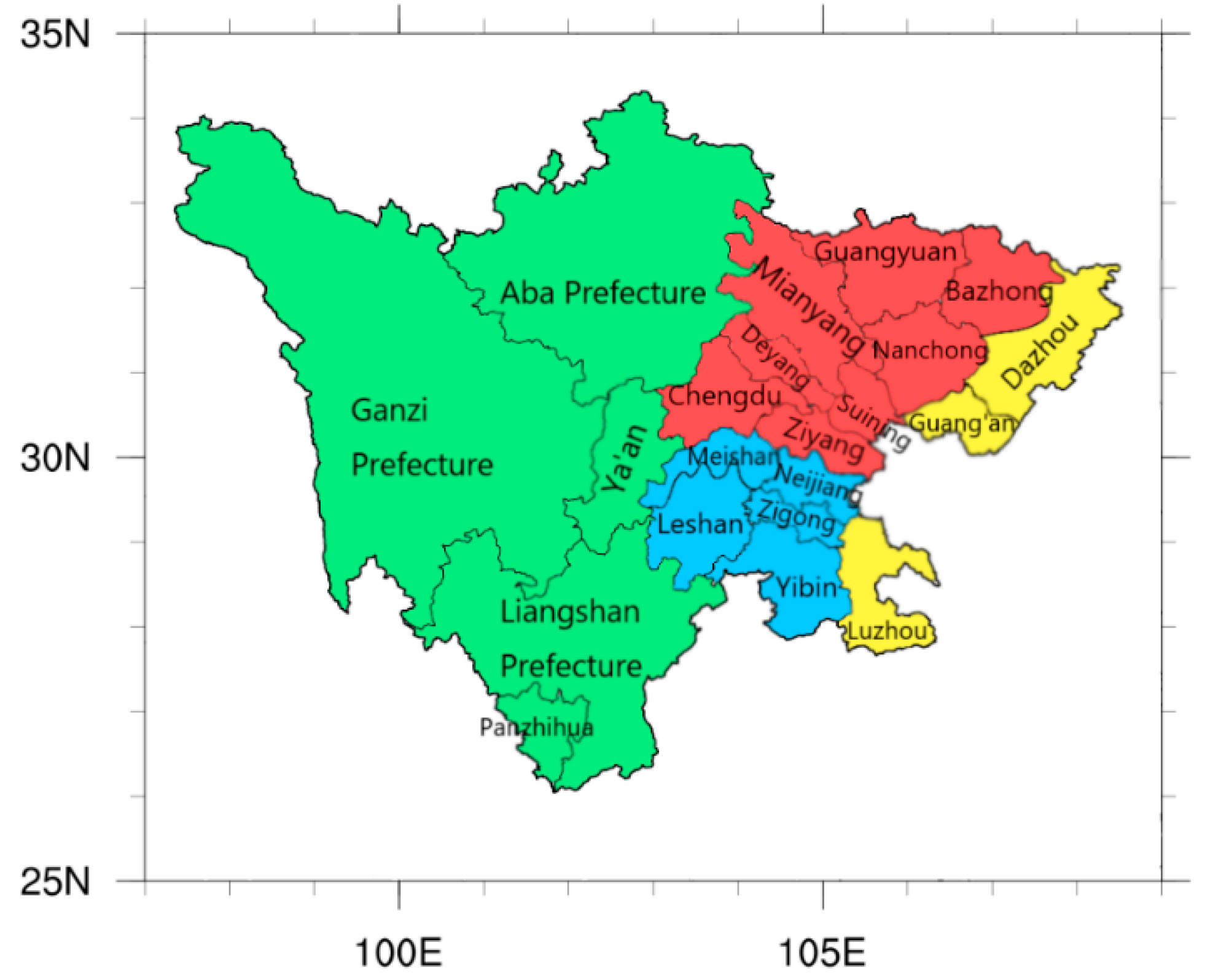
2.1. Study Area

Sichuan province (26°03′–34°19′ N, 97°21′–108°33′ E) is situated in southwest China. It is located in the transitional zone between the Qinghai–Tibet Plateau and the middle and lower reaches of the Yangtze River. It has four types of topography: mountains, hills, plains, and plateaus. Sichuan basin has a subtropical humid climate that features warm and wet weather, a long summer and a short winter, and abundant precipitation and sunshine.

2.2. Data Source

The data on pollution come from the environmental monitoring station of Sichuan province. They include the hourly AQI, hourly PM_2.5 (suspended particulates smaller than 2.5 µm in aerodynamic diameter), PM₁₀ (suspended particulates smaller than 10 µm in aerodynamic diameter), NO₂, SO₂, CO, and O₃ concentrations (μg/m³), and eight-hour O₃ concentrations (μg/m³) of 95 environmental monitoring stations in 21 cities in the Sichuan area. Particulate matter was measured using filter membrane samplers (HJ 93-2013) [12]. Other gaseous pollutants were measured using the continuous monitoring method (HJ 654-2013) [13]. All of the pollutants were measured per one hour except for O₃, which was taken as the average per eight hours, and all concentrations are accurate to two decimal places. The AQI was introduced to simplify the conventionally monitored air pollutant concentration (including fine particulate matter PM₁₀, respirable particulate matter PM_2.5, SO₂, NO₂, O₃ and CO) into a single conceptual value and grade the air pollution level and quality status according to the ambient air quality standard (GB3095-2012) [14] and the ambient AQI technical regulations (trial) (HJ 633-2012) [15] that were implemented by China’s Ministry of Environmental Protection in 2016.

The meteorological data, which include timed surface and sounding data from 19 December 2017 to 2 January 2018, come from the China Weather Network (www.weather.com.cn). The surface meteorological data that cover all ground meteorological observatories in 21 cities in Sichuan province include ground temperature (°C), wind speed (m/s), wind direction, and relative humidity (%) in every 3 hours at 02:00, 05:00, 08:00, 11:00, 14:00, 17:00, 20:00, and 23:00(all the times that mentioned in this paper are China Standard Time(abbreviated to CST), which is 8 hours earlier than the Coordinated Universal Time (UTC)). The timed sounding data include the vertical temperature distribution and vertical distribution of the K index and the SI index at 08:00 and 20:00 CST, showing the vertical structure in Yibin, Liangshan Prefecture, Ganzi, Dazhou, and Chengdu.

2.3. Methods

To study the impact of the most serious regional pollution process in Sichuan and its relationship to meteorological conditions, we first checked the distribution of variables using a cluster analysis. The results show that there is no significant difference between the pollutants’ concentrations in the Sichuan area. Thus, the 21 cities in Sichuan province can be divided into northern Sichuan (including Mianyang, Guangyuan, Bazhong, Nanchong, Deyang, Suining, Chengdu, and Ziyang), eastern Sichuan (including Dazhou, Guang’an, and Zhangzhou), southern Sichuan (including Meishan, Neijiang, Leshan, Zigong, and Yibin), and western Sichuan (including Aba, Ganzi, Liangshan, Panzhihua, and Ya’an) using administrative standards and topography patterns, as shown in Figure 1. Then, we analyzed the following three aspects.

2.3.1. Depiction of the Pollution Episode

In this part, hourly pollution data from 90 stations were first interpolated to the 21 cities’ meteorological stations, and then NCAR Command Language (NCL) [16] was used to plot the AQI and the concentration of each pollutant over time to describe the process. After that, the eight cities with the highest (maximum AQI) and lowest (minimum AQI) levels of pollution among the four regions were selected to study the hourly changes in concentration of the six pollutants (PM_2.5, PM₁₀, NO₂, SO₂, CO, and O₃) and further analyze the character of this pollution episode. The relationship between AQI value and air pollution level is shown in

Table 1. AQI category and health implications according to ambient air quality index (AQI) technical regulations (trial) (HJ 633-2012).

AQI	Air Pollution Level	Health Implications
0–50	Excellent	No health implications.
51–100	Good	Few hypersensitive individuals should reduce outdoor exercise.
101–150	Lightly Polluted	Slight irritations may occur, individuals with breathing or heart problems should reduce outdoor exercise.
151–200	Moderately Polluted	Slight irritations may occur, individuals with breathing or heart problems should reduce outdoor exercise.
201–300	Heavily Polluted	Healthy people will be noticeably affected. People with breathing or heart problems will experience reduced endurance in activities. These individuals and elders should remain indoors and restrict activities.
300+	Severely Polluted	Healthy people will experience reduced endurance in activities. There may be strong irritations and symptoms and may trigger other illnesses. Elders and the sick should remain indoors and avoid exercise. Healthy individuals should avoid outdoor activities.

.

Figures that reflect the changes in each pollutant over time and the ratio between the particle concentration and the concentration of NO₂ and SO₂ were made to describe the mutual conversion of pollutants and to analyze secondary formation reactions. Meanwhile, to determine whether photochemical reactions took place during this process, Pasquill–Turner stability (P-T stability) fractionation was used to analyze the fluctuation in ozone concentration and its changes over time according to the sunshine density data from the surface meteorological stations.

2.3.2. Meteorological Factors

In this part, we used the 500 hPa weather map to analyze the impacts of high- and low-pressure systems in high-altitude fields over China. Then, the Hybrid Single-Particle Lagrangian Integrated Trajectory (HYSPLIT) model was used to plot the backward trajectory to reflect the effect of external sources on local pollution in the later stages of the process. HYSPLIT is an atmospheric diffusion model that simulates air mass trajectory by using gridded meteorological data and the Lagrangian method to describe the motion of a flow point [17].

After analyzing the circulation and air mass trajectory, the conventional ground meteorological factors and their relationship to the hourly AQI were studied in the eight selected cities in the four regions.

Finally, to study the impact of boundary elements on the movement of contaminants, boundary layer height, ventilation, and vertical exchange coefficients were calculated from the sounding data. Boundary layer height refers to the thickness of the planetary boundary layer, which is related to atmospheric stability and wind speed. The larger the value is, the more favorable the vertical meteorological conditions are to facilitate the diffusion of pollutants and vice versa [16]. The Roche method was used to calculate the boundary layer height [18].

$$\mathrm{ABLH}=\frac{121}{6}\left(6-P\right)\left(T-T_d\right)+\frac{0.169P\left(U_Z+0.257\right)}{12f\ln \left(Z/Z_0\right)}$$

(1)

where ABLH is the atmospheric boundary layer height (m), P is the level of atmospheric stability (where the numbers 1–6 denote the levels A–F, respectively) graded by solar altitude, cloud cover, and surface wind speed, (T − T_d) is the dew point (K), and U_Z is the average wind speed at height Z(m) (m·s⁻¹). In this study, Z was taken to be 10. Z₀ is the surface roughness (m), since the established areas of the meteorological observations are located in the suburbs of cities that do not have large building blocks; in this study, Z₀ was taken to be 1. f is the geostrophic parameter (s⁻¹) obtained by the following formula:

$$f=2\mathsf{\Omega }\sin \mathsf{\Phi }$$

(2)

where Ω is the rotational angular velocity of the earth (7.292 × 10⁻⁵ rad/s), and Φ is the geographic latitude of the chosen location.

A ventilation index (VI) can be introduced to characterize the capacity to dilute and diffuse pollutants in the atmospheric boundary layer and denote the air quality and potentiality of pollution in a specific area. The larger the VI is, the stronger the atmospheric diffusion capacity is, resulting in better air quality in an area, and vice versa:

$$\mathrm{VI}=\mathrm{ABLH}\times U_{10}$$

(3)

where ABLH is the atmospheric boundary layer height (m) and U₁₀ is the horizontal wind speed 10 m above the ground.

The vertical exchange index (VEI) is related to air mass stability and the stability of stratification in the vertical atmosphere. It can be used to reflect the intensity of a vertical turbulent exchange on a large scale. The higher the value is, the greater the movement of a vertical turbulent exchange in the atmosphere is, and the easier it is for the atmosphere to be cleaned of contaminants [19].

$$\mathrm{VEI}={\left(0.84K-0.12SI+0.33LI\right)}^2$$

(4)

where K is the air mass index, SI is the Showalter index, and LI is the lifted index.

2.3.3. Correlation Analysis

In this part, the normality test was first used to detect the pollutant concentration. If the concentration of one of the six pollutants did not conform to a normal distribution, then the relationship between it and the meteorological factors (including the surface meteorological factors and the boundary layer factors) was analyzed by a Spearman correlation analysis. Otherwise, the Pearson method was chosen for the analysis.

3. Results and Discussion

3.1. Depiction of the Pollution Episode

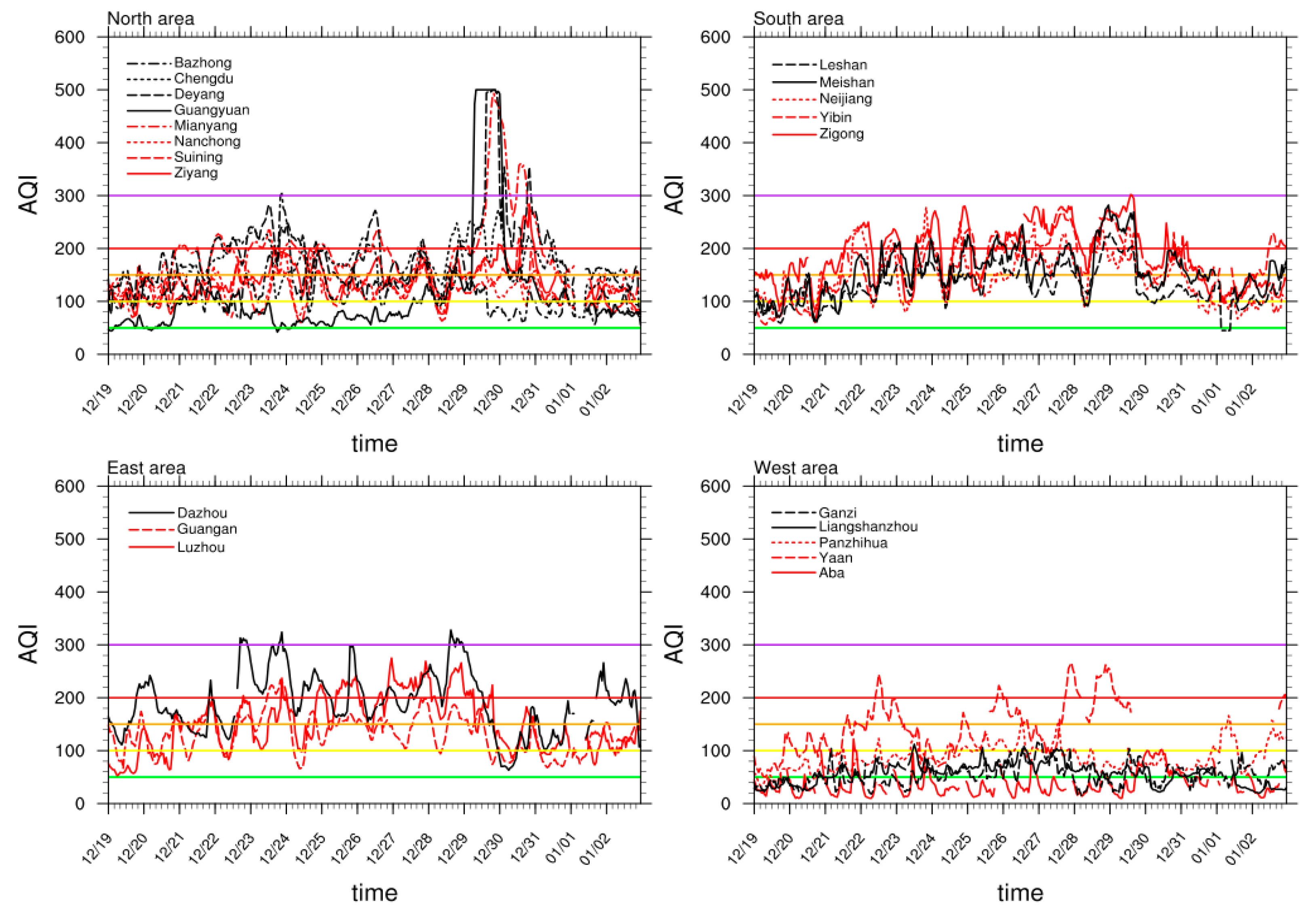
3.1.1. Analysis of AQI Variation

As shown in Figure 2, the pollution process began on 19 December 2017 and ended on 2 January 2018. The AQI in Guangyuan, Mianyang, and Deyang City in northern Sichuan increased to more than 490 from 29 to 30 December 2017, denoting the area that was most seriously affected during this pollution process. In other areas (such as southern and eastern Sichuan), the AQI was also greater than 200, indicating the widespread and serious impact that this pollution had on the region.

In addition to the western Sichuan Plateau, all other areas witnessed a smooth increase in AQI after 20 December 2017. The AQI in southern and eastern Sichuan reached 150 in a single day, and continued to increase from 22 to 30 December 2017, when it exceeded 200. Northern Sichuan was less polluted during this period. From 29 December 2017, the AQI in the northern area increased sharply to 500. After a diurnal change, the AQI plummeted, then rebounded slightly over 24 hours. Finally, the pollutants were cleared from the atmosphere and the AQI continued to drop until the end of the pollution process.

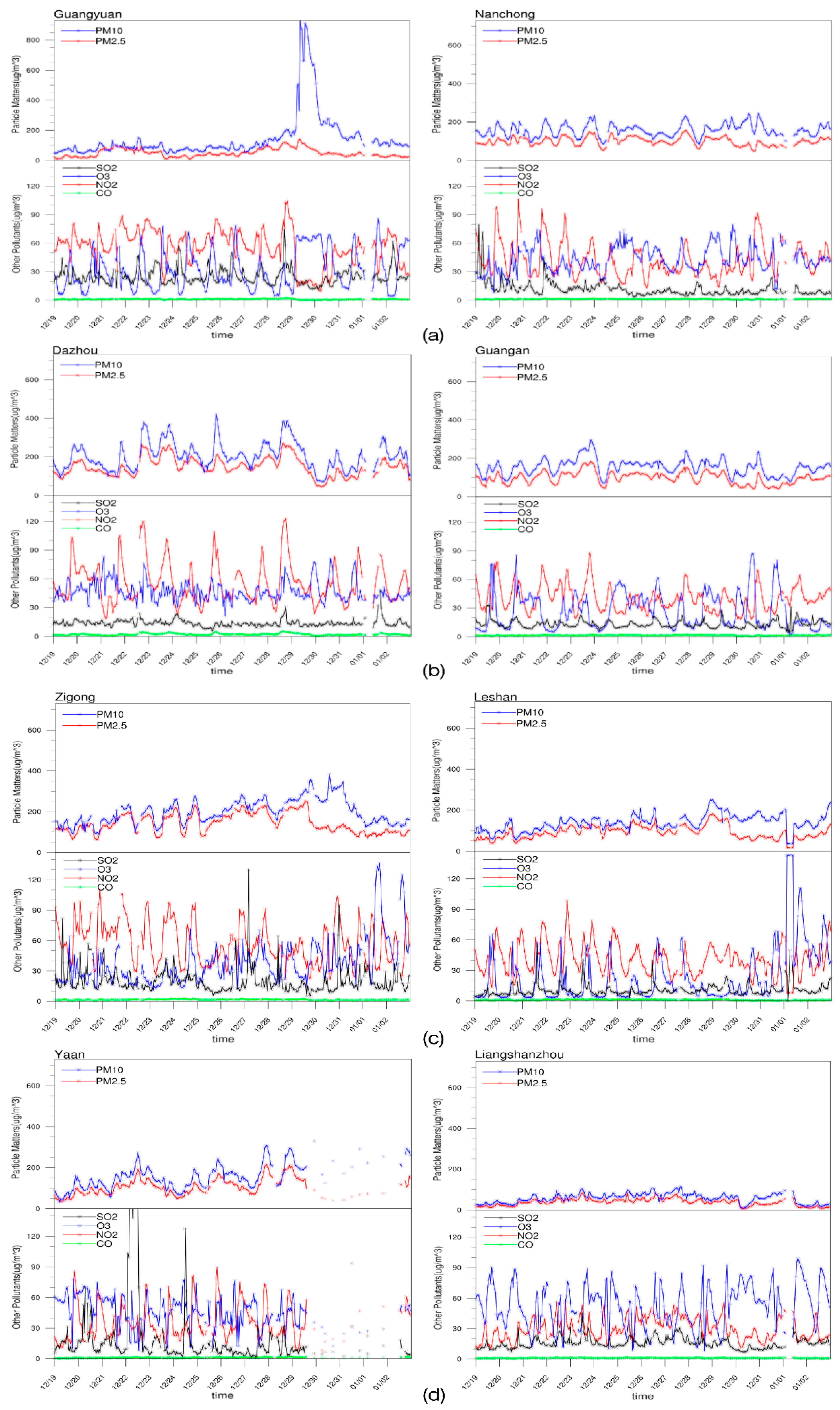
3.1.2. Analysis of Air Pollutants

Table 2. Hourly mass concentrations for PM₁₀ (µg/m³), PM_2.5 (µg/m³), NO₂ (µg/m³), SO₂ (µg/m³), O₃ (µg/m³) and the primary pollutants of each city during the process.

Region	City	PM10	PM2.5	NO2	CO	SO2	O3	AQI	AQImax	Primary Pollutants
Northern Sichuan	Mianyang	209.3	125.4	52.2	1.3	10.6	21.5	184.0	493	PM2.5
	Guangyuan	143.2	49.5	55.9	1.2	25.3	31.9	110.9	500	PM10
	Nanchong	157.3	99.5	41.9	1.2	11.7	43.1	113.5	206	PM2.5
	Ziyang	177.5	89.1	40.3	1.2	9.1	28.4	135.9	284	PM2.5 and PM10
	Deyang	223.1	127.0	65.5	1.3	9.4	20.7	186.5	499	PM2.5
	Suining	141.3	85.6	43.6	1.2	10.3	22.3	121.0	210	PM2.5
	Chengdu	197.5	120.9	71.1	1.4	14.6	31.6	116.9	273	PM2.5
	Bazhong	127.3	90.5	35.8	1.2	6.1	23.3	121.7	304	PM2.5
Eastern Sichuan	Guang’an	154.1	97.4	40.2	1.3	13.0	26.0	132.2	234	PM2.5
	Luzhou	174.7	110.9	59.9	1.2	19.5	19.0	151.8	275	PM2.5
	Dazhou	203.7	148.9	55.4	2.1	13.7	47.0	191.6	328	PM2.5
Southern Sichuan	Meishan	186.9	112.7	59.5	0.8	12.2	26.0	158.0	282	PM2.5
	Zigong	198.4	142.9	57.2	1.5	20.0	37.8	186.4	302	PM2.5
	Yibin	181.7	121.9	57.0	1.6	20.5	22.7	176.7	279	PM2.5
	Neijiang	158.2	107.5	45.6	1.2	29.0	29.0	146.5	278	PM2.5
	Leshan	139.2	91.6	40.9	1.1	10.7	23.3	127.9	229	PM2.5
Western Sichuan	Aba	36.7	18.5	13.7	0.6	11.1	42.2	37.1	122	PM2.5 and PM10
	Ganzi	51.7	32.8	15.8	0.4	14.4	63.1	54.2	116	PM2.5 and PM10
	Liangshan	57.4	37.6	29.7	1.0	15.7	52.7	57.1	112	PM2.5
	Panzhihua	116.4	55.2	58.3	2.6	39.5	29.3	86.4	166	PM10
	Ya’an	155.4	107.5	35.1	1.1	20.3	45.6	143.7	266	PM2.5

lists the average concentrations of the different pollutants and the maximum level during this pollution process in Sichuan. Table 2 and Figure 2 show that the most severely affected area was northern Sichuan, in which Guangyuan, Deyang, and Mianyang had peak AQI indices of 500, 499, and 493, respectively. The mass concentrations of PM₁₀ in Guangyuan, Deyang, and Mianyang were 143.2 μg/m³, 223.1 μg/m³, and 209.3 μg/m³, respectively. The average mass concentrations of PM_2.5 in Guangyuan, Deyang, and Mianyang were 49.5 μg/m³, 127.0 μg/m³, and 125.4 μg/m³, respectively. These results indicate that the pollution event in northern Sichuan was a particulate matter pollution event. In addition to the effect of particulate matter, the average SO₂ concentration in Guangyuan reached 25.3 μg/m³, which was the highest in northern Sichuan. The highest average O₃ concentration (43.1 μg/m³) was found in Nanchong, and the highest CO and NO₂ concentrations (1.4 μg/m³ and 71.1 μg/m³, respectively) were found in Chengdu. This was mainly due to the increase in the number of motor vehicles in urban areas, as SO₂, NO_X, and CO are mainly derived from the combustion of fossil fuels and motor vehicle emissions [20,21].

In the other regions, except for the strong variations in particulate matter concentration, the average mass concentration of CO and SO₂ in Panzhihua reached 2.6 μg/m³ and 39.5 μg/m³, respectively, representing the highest levels of these two pollutants in Sichuan. The average mass concentration of O₃ in Ganzi was 63.1 μg/m³, making ozone a strong secondary pollutant in this area.

The changes in the concentration of each pollutant over time are shown in Figure 3. It can be seen in Figure 3a that the concentration of PM₁₀ in Guangyuan increased sharply to 800 μg/m³ on 29 December 2017. The concentration of O₃ and SO₂ had daily periodic variation, and the maximum usually appeared in the afternoon. From 29 December 2017 onwards, the opposite trend was observed for these two gaseous pollutants. The change in pollutant concentration in Nanchong was weaker. The particulate matter concentration was low during the nighttime, high during the daytime, and peaked on 30 and 31 December 2017. The other pollutants had less-obvious patterns during the process.

Figure 3b shows that the concentration of particulate matter in Dazhou was high from 23 to 29 December 2017, with obvious daily variation and a maximum of 400 μg/m³. Meanwhile, the NO₂ concentration remained at a high level with a trend consistent with that of particulate matter: high during the nighttime and low during the daytime. The trend in Guang’an was similar to that in Nanchong, except that the particulate matter concentration first increased and then declined from 23 to 24 December 2017, and the ozone concentration in this area increased significantly on 30 December 2017.

In Zigong, the PM₁₀ concentration trend was not significant. The O₃ concentration slightly increased after 25 December 2017, picked up on 1 January 2018, and showed a significant upward trend over the next day. There were two significant changes in the SO₂ concentration during the nights of 27 December 2017 and 31 December 2017, respectively, both of which increased and then decreased quickly. Leshan had the same particulate matter concentration trend as Zigong. Other than particulate matter, the most obvious pollutant in Leshan was O₃, which changed daily before 28 December 2017 and fluctuated afterwards, reaching a maximum of 150 μg/m³ on 1 January 2018.

Figure 3d shows that, in western Sichuan, the most obvious change in pollutant concentration was SO₂ in Ya’an, which increased sharply between 22 and 23 December 2017 to 240 μg/m³. This was followed by changes in particulate matter concentrations that gradually increased after 29 December 2017 and peaked on 30 December 2017. The pollutants in Liangshan Prefecture remained at low levels. Only the ozone concentration remained relatively high (60 μg/m³) during the process.

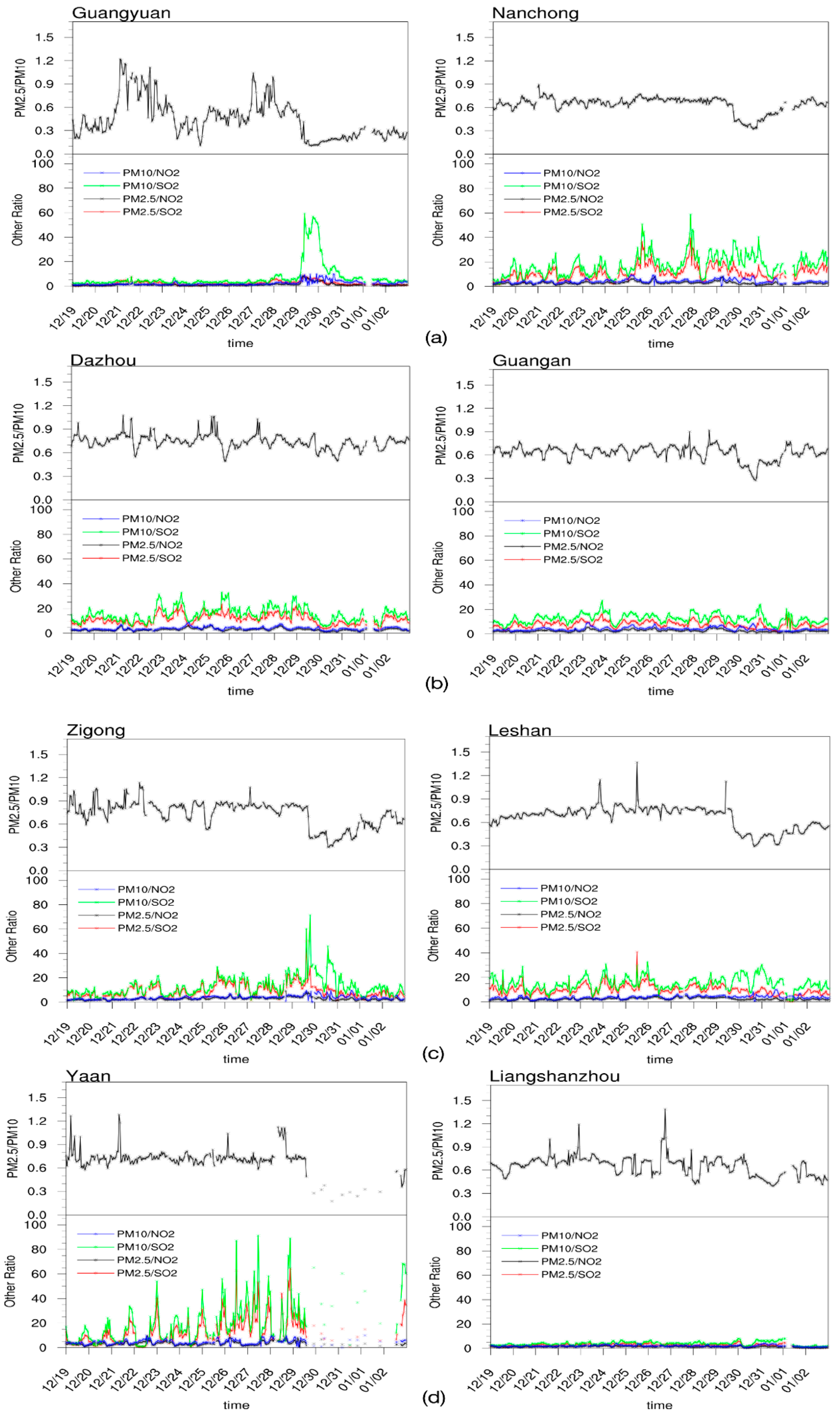
3.1.3. Secondary Formation

To analyze the mutual conversion of pollutants in the pollution process, this section compares the concentration of each pollutant in the eight cities.

As shown in Figure 4a, the ratio between the two types of particulate matter (PM_2.5/PM₁₀) in Guangyuan and Nanchong tended to rapidly decrease and gradually increase from 30 December 2017 to January 2018. The ratio between PM₁₀ and SO₂ in Guangyuan increased rapidly around 30 December 2017 and then decreased after one day. The ratio between particulate matter and SO₂ in Nanchong was maintained at a high level between 25 and 31 December 2017 due to the lower SO₂ concentration during this period, as shown in Figure 3. The most obvious fluctuation in the pollutant concentration in northern Sichuan occurred from 30 to 31 December 2017, represented by a sudden increase in PM₁₀ concentration in most parts of this area.

The PM_2.5/PM₁₀ ratio in Dazhou remained at a high level from 20 December 2017 to 1 January 2018. The same ratio in Guang’an was low, and dropped sharply on 30 December 2017 as the concentration of fine particles significantly decreased on the same day. Figure 4c shows the trend of pollutants in Zigong and Leshan in southern Sichuan, which plummeted on 31 December 2017 and slowly decreased thereafter. In both areas, there was a tendency for the coarse particle concentration to increase and the fine particle concentration to decrease.

As can be seen in Figure 4d, the ratios of particulate matter and SO₂ in Ya’an fluctuated greatly and were low in the daytime and high in the nighttime from 20 December 2017. Between 26 and 30 December 2017, the conversion frequency became higher, then was gradually reduced on 2 January 2018. The trend in Liangshan Prefecture was slightly different, in which the PM₁₀ concentration increased slightly, and the PM_2.5 concentration decreased significantly after 30 December 2017.

According to Wang (2014), when the relative humidity is greater than 50%, SO₂ and NO₂ will be oxidized to SO₄²⁻ and NO₃⁻, respectively [21]. The aerosol’s hygroscopic growth effect will also change the particle size distribution and optical properties under different relative humidities; that is, the higher the relative humidity is, the more PM_2.5 there is in the atmosphere [22]. During the pollution process, the relative humidity of each of the eight cities was higher than 50%, which was conducive to the oxidation of SO₂ and NO₂ and reduced their concentration. However, the relative humidity decreased significantly in all eight cities from 30 to 31 December 2017, inhibiting the growth of PM_2.5. This resulted in a decrease in the ratio between the two particulate matter types. As PM_2.5/PM₁₀ provides an indication of the particle size in the ash process [23], we can conclude that fine particle pollution dominated this episode at the end of December.

The sunshine level that was obtained from the P-T stability fractionation, as shown in Figure 5. The sunshine level in Nanchong and Guang’an increased significantly on 1 January 2018. From Figure 3, we can conclude that photochemical reactions occurred in these cities and produced more O₃. However, there was also a sudden increase in ozone concentration in southern Sichuan from 1 to 2 January 2018, when the sunshine level was maintained at level 3. These results, combined with the study of Yan Yulong (2016), indicate that the sudden increase in ozone concentration in southern Sichuan was mainly due to the growing concentration of NO₂ and SO₂ that was caused by a secondary transformation to inorganic ions [23].

It can be comprehensively concluded that the PM_2.5 concentration in northern Sichuan decreased, and the PM₁₀ concentration increased sharply, after 30 December 2017. In addition, the concentration of fine particulate matter in the eastern, western, and southern parts of Sichuan decreased dramatically and then recovered slowly due to the change in relative humidity that affected the particle size distribution. There was a sudden increase in ozone concentration on 1 January 2018 in northern Sichuan as well as in southern Sichuan, which relied mainly on precursor NO₂ and SO₂ and the solar radiation level.

3.2. Meteorological Factors

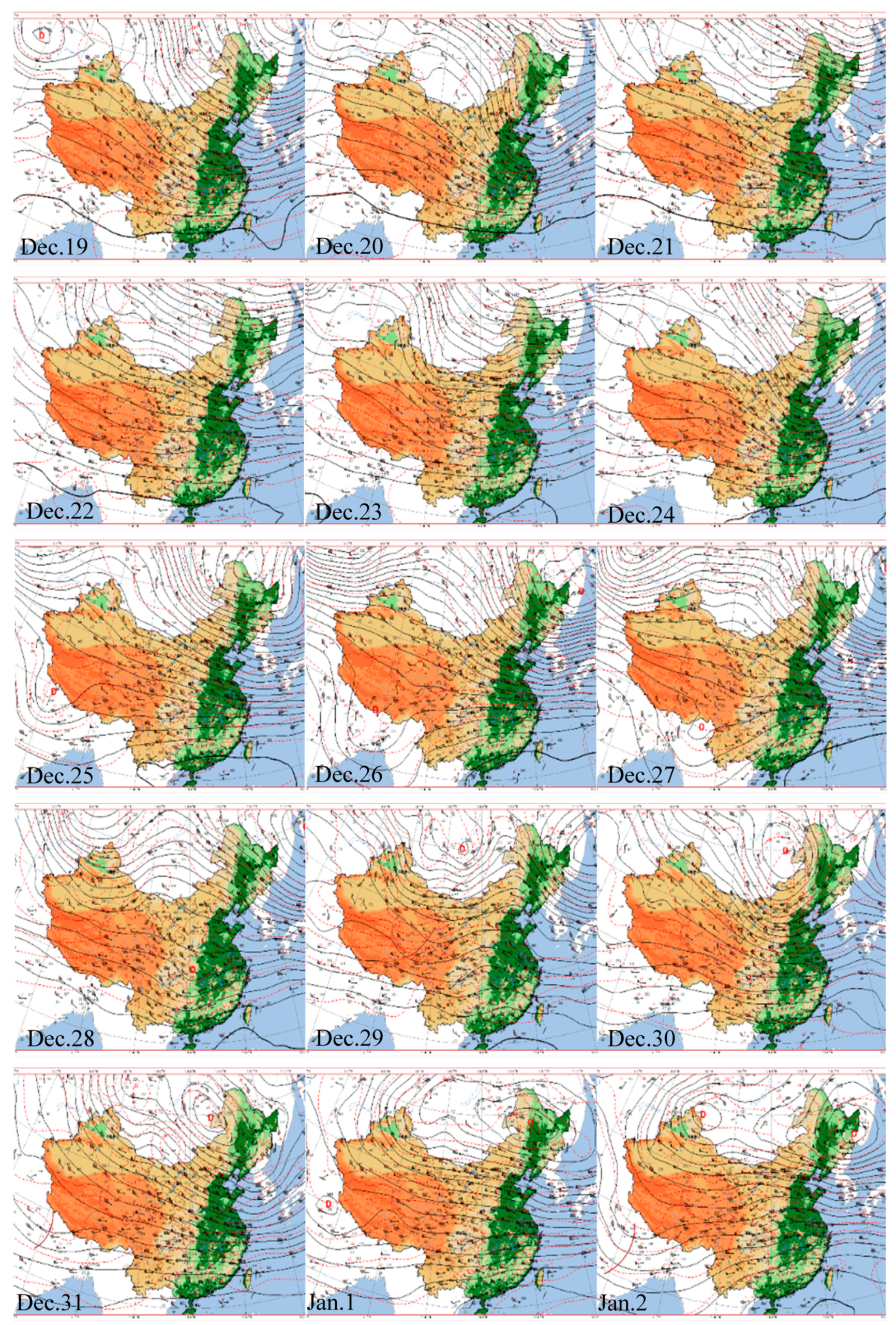
3.2.1. Synoptic Circulation

As shown in Figure 6, Sichuan experienced three major fluctuations at 500 hPa during this 15-day pollution process. The first event occurred from 22 to 24 December 2017, when small fluctuations in the central part of the Qinghai–Tibet Plateau moved eastward to affect the northern part of the Sichuan basin, transforming the upper part of the circulation over northern Sichuan to a downdraft. The second event occurred from 25 to 28 December 2017, and was caused by the eastward movement of a low-pressure system in the Sino-Indian Peninsula that produced the same change to the entire Sichuan area as the first fluctuation did. During this time, the third event began in the middle of the plateau, the low trough of which moved eastward through the Sichuan Basin. A low-pressure system formed in western Mongolia that drove cold air to the south and affected China by moving eastward. On 2 January 2017, the pressure center was split in northwestern China, brought continuous cold air to western China, and initiated this heavy pollution episode.

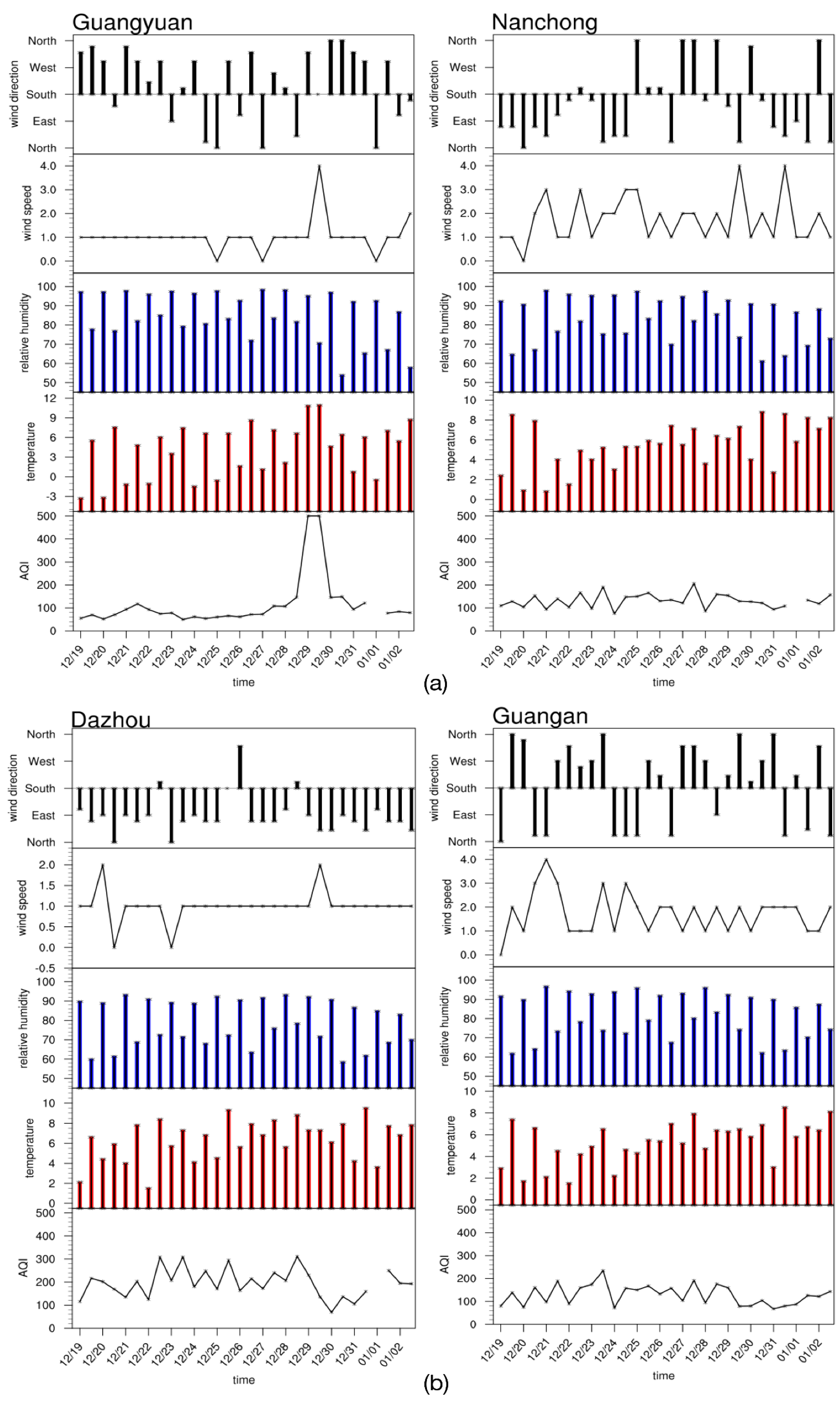
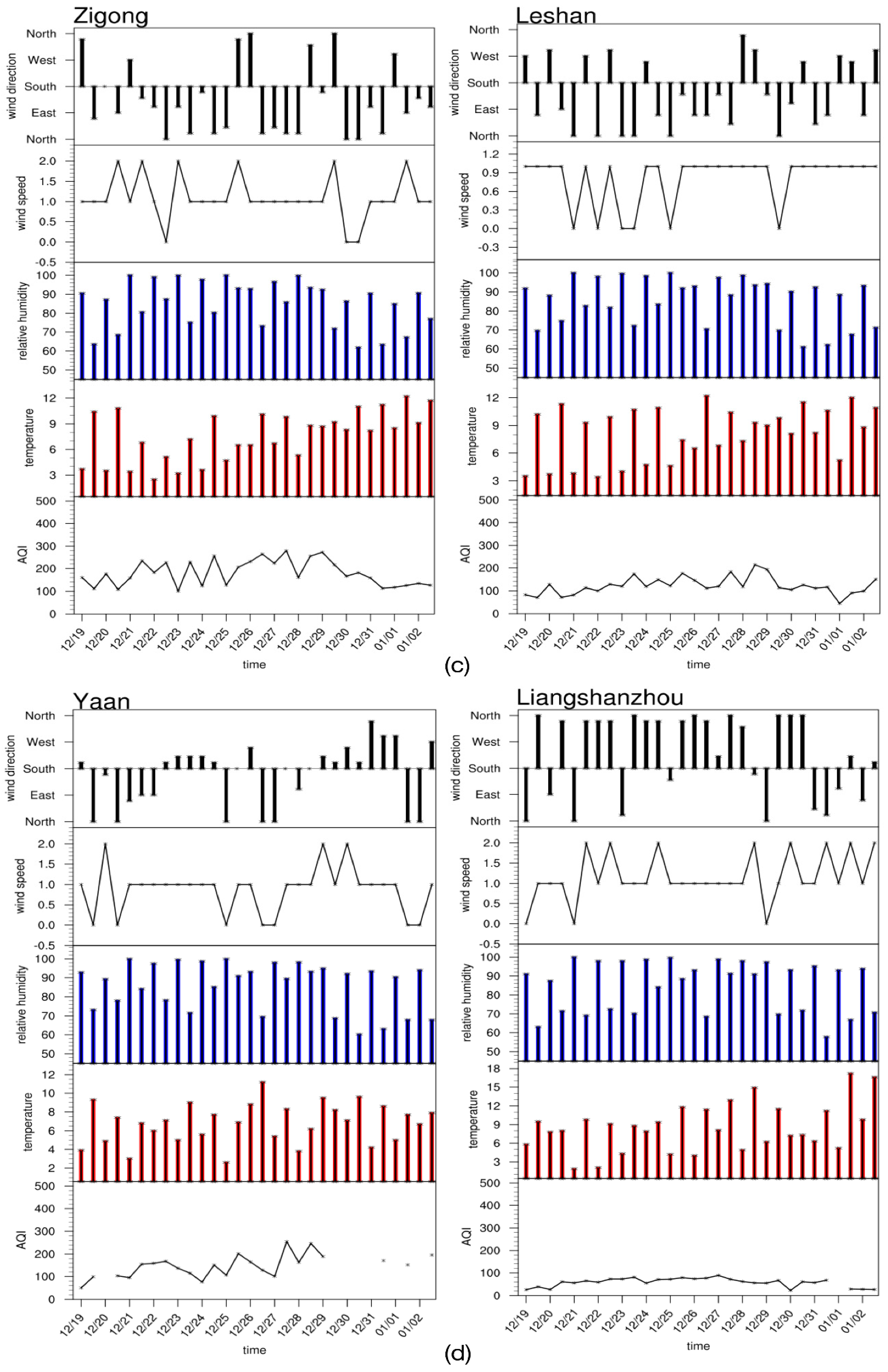
3.2.2. Surface Meteorological Factors

In this section, we analyze the surface meteorological elements (including wind direction, wind speed, relative humidity, and ground temperature) in the eight chosen cities.

As shown in Figure 7a, the maximum AQI in Guangyuan occurred on 30 December 2017, when there was a strong northerly ground wind, the relative humidity dropped to 55% at night, and the ground temperature remained the same. The AQI in Nanchong had no obvious change when there was a northerly wind (<1 m/s), the relative humidity increased, and the ground temperature decreased.

As shown in Figure 7b, the AQI in Dazhou and Guang’an increased and then stabilized from 21 to 29 December 2017. The maximum AQI in Dazhou was maintained at approximately 200 when weak winds and a high relative humidity dominated this area. The situation in Guang’an was the same. The distribution of the AQI in southern Sichuan, represented by Zigong and Leshan, was similar to that in eastern Sichuan. As shown in Figure 7c, both Zigong and Leshan were dominated by small winds, the relative humidity first increased and then decreased, and the ground temperature increased slowly during this period of time.

Western Sichuan was the least polluted area. Ya’an’s AQI increased from 21 to 29 December 2017, during which time Ya’an had small northerly winds, an increased relative humidity, and a decreased ground temperature. The ground elements in Liangshan Prefecture were similar to those of Ya’an, except that the overall level was lower.

Wang et al. (2014) pointed out that a low wind speed and high relative humidity in the near-surface layer are closely related to the occurrence and persistence of heavy regional pollution [24]. Therefore, the persistent heavy pollution in eastern and southern Sichuan from 21 to 30 December 2017 can be mainly attributed to atmospheric stratification that was not conducive to the spread of pollution. On the other hand, in western Sichuan, there was stable atmospheric stratification before 30 December 2017, which was conducive to the deliquescence, composition, and maintenance of local secondary formations, thus worsening the air quality [25].

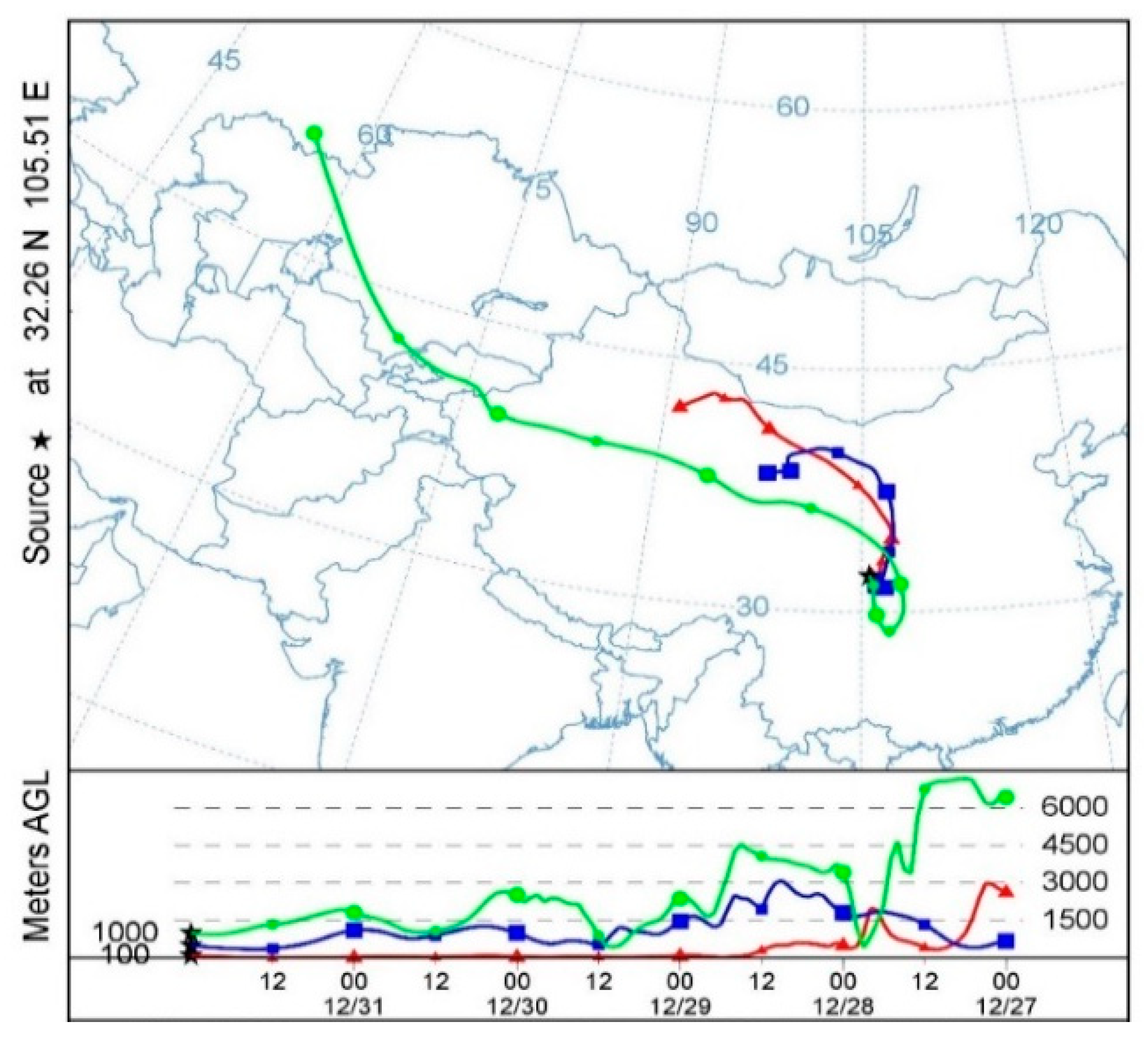
3.2.3. Air Mass Backward Trajectory Analysis

The air mass trajectory over the Guangyuan area in northern Sichuan from 27 December 2017 to 1 January 2018 was calculated using the HYSPLIT backward trajectory model, and the external source in this process was analyzed.

As shown in Figure 8, over the Guangyuan area, the air mass in the upper atmosphere (1000 m) originated from Kazakhstan. The air mass in the middle layer (500 m) was from the Gansu-Qinghai area, whereas the near-surface air mass (100 m) originated from northern Xinjiang. These results, combined with the analysis of the 500 hPa field, suggest that the sudden increase in PM₁₀ concentration on 30 December 2017 was due to the air mass over Guangyuan being guided by the northwest airflow of the low-pressure system that carried sand and dust into Sichuan, forming a serious particulate matter pollution process in northern Sichuan on 30 December 2017.

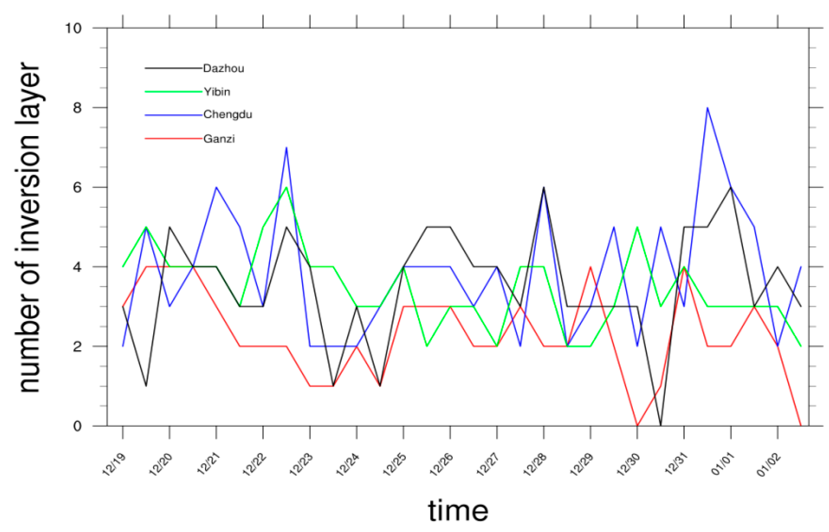
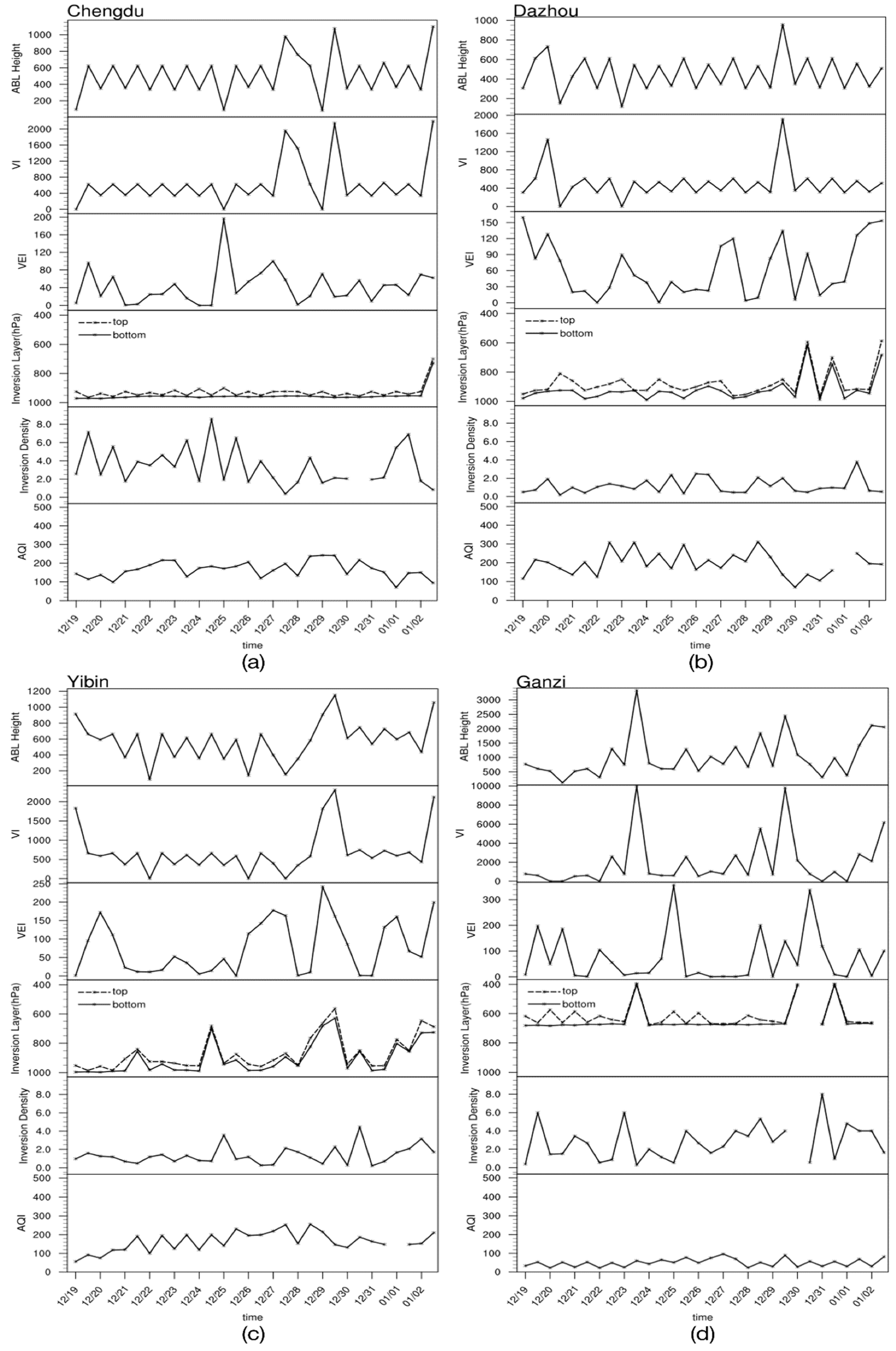
3.2.4. Atmospheric Boundary Layer

There are five sounding stations in Sichuan Province, among which the Ganzi, Dazhou, Yibin, and Chengdu stations were chosen to represent the four regions of Sichuan. The inversion layer distribution maps over different stations were obtained by calculating the vertical temperature distribution and the atmospheric stability index for each layer.

As shown in Figure 9, there was always more than two inversion layers over the Chengdu area, and eight inversions even appeared on the nights of 22 and 30 December 2017, suppressing the vertical exchange in the atmosphere and making it difficult for the pollutants to spread. The inversion in Yibin and Dazhou averaged 1–5 layers, while Ganzi station had fewer inversion layers; only four layers occurred during the daytime from 19 to 20 December 2017.

To study the effects of the boundary layer on pollutant transport, the sounding data were calculated to obtain the ABLH, VI, VEI and the height of the bottom and the top of the first inversion over time. The results can be seen from Figure 10.

Chengdu experienced severe pollution from 21 to 31 December 2017 (AQI > 200). During this time, the boundary layer was low (200–600 m), and the VI and VEI were stable at 800 m²/s and below 100, respectively, which were not conducive to the vertical and horizontal diffusion of pollutants. Then, the VI and the ABLH increased to 1000 m, improving the horizontal turbulent exchange and removing the pollutants. The bottom of the inversion layer above the Chengdu area was always close to the ground (950 hPa), and the strength of the first inversion layer was 2 °C/100 m, strongly inhibiting the vertical diffusion of pollutants. According to Zhang (2017), static winds, a low boundary layer, a strong inversion layer, and high relative humidity are conducive to the formation of antimony pollution [26]. Therefore, in northern Sichuan, as represented by Chengdu station, the severe air pollution from 21 to 31 December 2017 was mainly affected by the static weather.

Dazhou and Yibin were both severely polluted from 21 to 29 December 2017, and had a slightly more active atmosphere compared to Chengdu. Their boundary layer conditions were stable until 29 December 2017, when the vertical and horizontal atmospheric turbulence strengthened and the pollutants were removed. On the other hand, western Sichuan, as represented by Ganzi station, was less polluted during the process (AQI < 100). All boundary layers’ factors were conducive to the diffusion of pollutants, except for the strong inversion intensity (up to 8 °C/100 m).

To conclude, the boundary layer height over Sichuan was low and the inversion layers suppressed energy in the near-surface layer, which in turn facilitated the accumulation of pollutants [27]. The weak turbulent exchange inhibited the diffusion of pollutants, causing Sichuan to be continuously polluted until the stable atmospheric stratification was broken, the inversion layer collapsed, and the atmospheric turbulence was strengthened, at which point the air quality recovered.

3.3. Relationship between Air Pollutants and Meteorological Factors

After the normality test, only the concentrations of PM₁₀, CO, and O₃ had a normal distribution, whereas the other pollutants (PM_2.5, NO₂, and SO₂) deviated from a linear distribution. Therefore, the nonparametric Spearman correlation analysis was used to improve the accuracy. The results are shown in

Table 3. The correlation coefficients between the concentrations of pollutants and meteorological factors in the eight chosen cities. The numbers in red represent strong correlations (|R| > 0.5) between the corresponding variables.

	City		PM2.5	PM10	CO	NO2	O3	SO2
Northern Sichuan	Guangyuan	Wind Speed	0.058	0.258 *	−0.364 *	−0.290 *	0.476 *	−0.025
		Relative Humidity	0.064	0.346	0.220	−0.183	−0.613 *	−0.180
		Temperature	0.058	0.352 *	−0.249 *	−0.221 *	0.691 *	−0.032
		ABL	−0.037	0.292 *	−0.490 *	−0.318 *	0.666 *	0.003
		VI	0.017	0.312 *	−0.466 *	−0.355 *	0.649 *	−0.010
		VEI	−0.118	0.100	−0.031	0.089	0.092	0.032
	Nanchong	Wind Speed	0.023	0.047	−0.079	−0.206 *	0.406 *	−0.043
		Relative Humidity	−0.404 *	−0.629	−0.473 *	−0.809	−0.391 *	0.323
		Temperature	0.121	0.270 *	−0.081	0.235 *	0.282 *	−0.396 *
		ABL	−0.006	0.136	−0.168	−0.079	0.381 *	−0.081
		VI	0.028	0.151	−0.128	−0.083	0.425 *	−0.091
		VEI	0.245	0.158	−0.081	0.121	0.045	−0.400 *
Eastern Sichuan	Dazhou	Wind Speed	−0.108	−0.085	−0.111	−0.107	0.197 *	−0.045
		Relative Humidity	−0.255	−0.462 *	−0.165	−0.668 *	−0.253	−0.107
		Temperature	0.224 *	0.308 *	−0.268 *	0.492 *	0.303 *	0.013
		ABL	0.003	0.093	−0.028	0.253 *	0.367 *	0.003
		VI	0.031	0.107	−0.030	0.187 *	0.313 *	0.014
		VEI	−0.017	0.001	0.045	0.043	−0.026	−0.290
	Guang’an	Wind Speed	0.076	0.101	0.118	0.189 *	0.111	0.116
		Relative Humidity	−0.265	−0.272	0.137	−0.540 *	−0.255	−0.101
		Temperature	0.053	0.103	0.072	0.199 *	0.109	0.224 *
		ABL	0.083	0.094	0.030	0.091	0.087	−0.109
		VI	0.070	0.105	0.094	0.196 *	0.120	0.114
		VEI	−0.101	−0.101	−0.055	0.188	−0.285	0.197
Southern Sichuan	Zigong	Wind Speed	−0.054	−0.074	0.083	0.081	0.116	0.131
		Relative Humidity	0.055	−0.314	0.306	−0.742 *	−0.454 *	0.202
		Temperature	−0.072	−0.006	−0.005	0.132	0.207 *	0.045
		ABL	−0.019	0.006	0.002	0.151	0.187 *	0.079
		VI	−0.075	−0.066	0.041	0.095	0.158	0.110
		VEI	0.027	0.011	−0.039	0.096	0.115	−0.141
	Leshan	Wind Speed	−0.087	0.127	−0.294 *	−0.204 *	0.309 *	0.160
		Relative Humidity	0.223	−0.193	0.293	−0.601 *	−0.737 *	−0.153
		Temperature	−0.011	0.253 *	0.323 *	0.148	0.782 *	0.427 *
		ABL	−0.173	0.169	−0.488 *	0.026	0.617 *	0.280 *
		VI	−0.167	0.163	−0.463 *	0.015	0.579 *	0.269 *
		VEI	0.143	0.060	0.103	−0.117	0.204	0.165
Western Sichuan	Ya’an	Wind Speed	−0.167	−0.187	−0.315 *	−0.537 *	−0.029	0.157
		Relative Humidity	0.070	−0.522 *	−0.491 *	−0.589 *	0.034	0.348
		Temperature	0.019	0.134	0.026	−0.147	−0.244 *	−0.026
		ABL	−0.162	−0.111	−0.319 *	−0.486 *	−0.087	0.049
		VI	−0.161	−0.125	−0.315 *	−0.510 *	−0.103	0.105
		VEI	0.181	0.145	0.156	0.154	−0.165	−0.234
	Liangshan	Wind Speed	−0.192 *	−0.206 *	−0.260 *	−0.160	0.422 *	0.075
		Relative Humidity	−0.017	0.012	0.386 *	0.321	−0.742 *	−0.043
		Temperature	0.098	−0.072	−0.280 *	−0.129	0.420 *	0.439 *
		ABL	−0.350 *	−0.318 *	−0.430 *	−0.384 *	0.526 *	0.182
		VI	−0.340 *	−0.322 *	−0.412 *	−0.343 *	0.553 *	0.148
		VEI	−0.153	0.159	0.043	0.083	0.055	0.199

* p < 0.05: the result is significant.

.

In northern Sichuan, O₃ was the most-correlated pollutant to meteorological elements and boundary layer conditions in Guangyuan, which correlated to the precursors volatile organic compounds (VOC) and NO_X and the ground temperature that reflects the intensity of sunshine [28,29]. Nanchong, however, had different correlation trends, in which the strongest correlation occurred between NO₂ and PM₁₀ and relative humidity, the other pollutants and meteorological factors were moderately correlated, and the coefficients were not highly significant.

The general correlations between meteorological elements and pollutants in Dazhou were weaker. Only relative humidity and NO₂ were highly related (R = −0.668, p < 0.05); the same was found for Guang’an (R = −0.504, p < 0.05), Zigong (R = −0.742, p < 0.05), and Ya’an (R = −0.589, p < 0.05). Thus, in those areas, more NOx gas underwent secondary conversion to form NO₃⁻ with an increase in relative humidity [21], a reduction in NO₂ concentration, and suppression of ozone generation.

In Leshan, the strongest correlation appeared for ozone and ground temperature (R = −0.782, p < 0.05). The O₃ concentration in Liangshan Prefecture was closely related to relative humidity and weakly related to boundary layer elements; that is, the ozone in the atmosphere was mainly controlled by surface meteorological factors. On the other hand, factors in the boundary layer (except for the VEI) over Liangshanzhou were closely related to the concentration of other pollutants. This indicates that the motion of the atmospheric boundary layer had a significant influence on the transmission and diffusion of pollutants other than ozone.

In conclusion, during this process of pollution, the surface meteorological and boundary layer elements had a significant impact on the concentration of pollutants, mainly affecting photochemical reactions and changing the concentration of ozone through changes in surface meteorological factors and the turbulence exchange in the atmosphere.

3.4. Discussion

Generally, this study provides a broader analysis of a pollution episode that involves the effects of surface factors and boundary layer conditions. The results on the effects of meteorological factors on pollutants’ properties are consistent with those of other studies. Ning et al. (2018) studied the impacts of low-pressure systems on air pollution events in northwest Sichuan during winter, and found that a stagnant situation before a low-pressure system benefits the accumulation of pollutants, while, after the low-pressure system, pollutants are likely to be removed by the strengthening wind conditions and the vertical exchange in the atmosphere [30]. Liao et al. (2018) also focused on the stagnation effects on southwestern China [31], while Zhang et al. (2019) studied Sichuan Basin’s terrain effects [32]. Both studies obtain a relationship between pollutants’ properties and meteorological factors similar to that obtained by Ning et al. (2018). Ning et al. (2018) showed that particulate matter patterns are mostly related to meteorological factors, while gaseous pollutant patterns mainly depend on the distribution of emission sources [33]. However, there is a limited number of studies on the relationship between gaseous pollutants and meteorological factors in Sichuan. According to Elminir (2005), in the entire territory of Great Cairo, a higher particulate pollution level can be attributed to a high wind speed, and an intense sunlight level and low relative humidity are favorable for NO₂ and O₃, which is consistent with our result [34].

4. Conclusions

• This pollution process began on 19 December 2017 and ended on 2 January 2018. The main pollution area switched from southeastern Sichuan to northern Sichuan because of the growing effects of external sources. The main pollutants were PM_2.5 and PM₁₀ over all of the cities; however, in addition to particulate matter, some cites experienced a concentration burst in specific kinds of pollutants due to motor vehicle exhaust emissions (such as NO₂ in Chengdu), the combustion of core fuel (such as CO and SO₂ in Panzhihua), and photochemical reactions (such as O₃ in Ganzi).
• With respect to circulation, Sichuan experienced ridges that moved eastward across the basin three times and changed the local circulation pattern. Meanwhile, ground meteorological factors (specifically, a low wind speed and high relative humidity) were also conducive to the accumulation of pollutants, resulting in a continuous increase in the pollutants’ concentrations. On 30 December 2017, a low-pressure system that formed in Mongolia brought dust into Sichuan and increased the concentration of particulate matter in the northern region. The atmospheric conditions in other areas became unstable because of the incoming cold air, the pollutants were removed, and the pollution process ended.
• In this pollution process, the most closely related variables between the pollutant concentration and meteorological elements were NO₂ and O₃ with the ground relative humidity and temperature, the boundary layer height, and the VI. The precursors that were generated from the motor vehicle emissions and coal-fired processes in winter affected the photochemical conversion process in the atmosphere with a high ground temperature and low relative humidity, resulting in a high ozone concentration.

References

1. Kang, H.; Zhu, B.; Su, J.; Wang, H.; Zhang, Q.; Wang, F. Analysis of a long-lasting haze episode in Nanjing, China. Atmos. Res. 2013, 120–121, 78–87. [Google Scholar] [CrossRef]
2. Tian, G.; Qiao, Z.; Xu, X. Characteristics of particulate matter (PM10) and its relationship with meteorological factors during 2001–2012 in Beijing. Environ. Pollut. 2014, 192, 266–274. [Google Scholar] [CrossRef] [PubMed]
3. Bei, N.; Zhao, L.; Xiao, B.; Meng, N.; Feng, T. Impacts of local circulations on the wintertime air pollution in the Guanzhong Basin. China Sci. Total Environ. 2014, 592, 373–390. [Google Scholar] [CrossRef]
4. Wikipedia. Available online: https://en.wikipedia.org/wiki/Air_pollution_episode (accessed on 10 March 2019).
5. Zeng, S.; Zhang, Y. The Effect of Meteorological Elements on Continuing Heavy Air Pollution: A Case Study in the Chengdu Area during the 2014 Spring Festival. Atmosphere 2017, 8, 71. [Google Scholar] [CrossRef]
6. Ning, Z.; Liu, H. Domestic and Abroad Research Status of Atmospheric Boundary Layer. J. EMCC 2017, 27, 12–15. [Google Scholar]
7. Kallos, G.; Kassomenos, P.; Pielke, R.A. Transport and Diffusion in Turbulent Fields; Kluwer Academic Publishers: Dordrecht, The Netherlands, 1993; pp. 163–184. [Google Scholar]
8. Zhang, Y.; Liu, Z.; Lv, X.; Zhang, Y.; Qian, J. Characteristics of the transport of a typical pollution event in the Chengdu area based on remote sensing data and numerical simulations. Atmosphere 2016, 7, 127. [Google Scholar] [CrossRef]
9. Guo, X. Observed and Simulated Research on Climate Characteristic of Air Quality and the Topographic Induced Effects in Sichuan Basin. Master’s Thesis, Nanjing University of Information Science & Technology, Nanjing, China, 2016. [Google Scholar]
10. Yu, W.; Luo, X.; Fan, S.; Liu, J.; Feng, Y.; Fan, Q. Characteristics Analysis and Numerical Simulation Study of a Severe Air Pollution Episode over the Pearl River Delta. Res. Environ. Sci. 2011, 24, 645–653. [Google Scholar] [CrossRef]
11. Zhang, P.; Jin, Q.; Lu, X.; Li, C.; Jiang, Y. Analysis on environmental factors affecting air pollution in a durative haze weather in January 2013. J. Meteorol. Sci. 2016, 36, 112–120. [Google Scholar]
12. The Ministry of Environmental Protection (MEP). Specifications and Test Procedures for PM10 and PM2.5 Sampler; HJ 93-2013; The Ministry of Environmental Protection (MEP): Beijing, China, 2013; pp. 1–15. [Google Scholar]
13. The Ministry of Environmental Protection (MEP). Specifications and Test Procedures for Ambient Air Quality Continuous Automated Monitoring System for SO2 NO2 O3 and CO; HJ 654-2013; The Ministry of Environmental Protection (MEP): Beijing, China, 2013; pp. 1–19. [Google Scholar]
14. The Ministry of Environmental Protection (MEP). Ambient Air Quality Standard; GB3095-2012; The Ministry of Environmental Protection (MEP): Beijing, China, 2012; pp. 2–3. [Google Scholar]
15. The Ministry of Environmental Protection (MEP). Technical Regulation on Ambient Air Quality Index (on Trial); HJ 633-2012; The Ministry of Environmental Protection (MEP): Beijing, China, 2012; pp. 2–4. [Google Scholar]
16. The NCAR Command Language (Version 6.4.0); UCAR/NCAR/CISL/TDD: Boulder, CO, USA, 2017.
17. Wang, J.; Ogawa, S. Effects of meteorological conditions on PM2.5 concentrations in Nagasaki, Japan. Int. J. Environ. Res. Public Health 2015, 12, 9089–9101. [Google Scholar] [CrossRef] [PubMed]
18. Zhang, H.; Lv, M.; Zhang, B.; An, L.; Rao, X. Analysis of the stagnant meteorological situation and the transmission condition of continuous heavy pollution course from 20–26 February 2014 in Beijing-Tianjin-Hebei. Acta Sci. Circumst. 2016, 36, 4340–4351. [Google Scholar]
19. Nozaki, K.Y. Mixing Depth Model Using Hourly Surface Observations; Report 7053; USAF Environmental Technical Applications Center: Washington, DC, USA, 1973. [Google Scholar]
20. Li, Z.; Chen, J.; Du, Y.; Wang, B. Characteristics of Regional Air Pollution Process in Chengdu and Surrounding Areas. Environ. Sci. Technol. 2015, 38, 125–130. [Google Scholar] [CrossRef]
21. Wang, Y.; Yao, L.; Wang, L.; Liu, Z.; Ji, D.; Tang, G.; Zhang, J.; Sun, Y.; Hu, B.; Xin, J. Mechanism for the formation of the January 2013 heavy haze pollution episode over central and eastern China. Sci. China Earth Sci. 2014, 57, 14–25. [Google Scholar] [CrossRef]
22. Wang, S.; Liao, T.; Wang, L.; Fan, C.; Xu, J.; Sun, Y. Atmospheric characteristics of a serious haze episode in Xi’an and the influence of meteorological conditions. Acta Sci. Circumst. 2015, 35, 3452–3462. [Google Scholar]
23. Wu, D.; Wu, S.; Li, H.; Chen, H. Analysis of the typical haze process in the pearl river delta from 17–23 March 2010. Res. Environ. Sci. 2011, 31, 695–703. [Google Scholar] [CrossRef]
24. Wang, Y.; Wang, L.; Zhao, G.; Wang, Y.; An, J.; Liu, Z.; Tang, G. Analysis of Different-Scales Circulation Patterns and Boundary Layer Structure of PM2.5 Heavy Pollutions in Beijing during Winter. Clim. Environ. Res. 2014, 19, 173–184. (In Chinese) [Google Scholar]
25. Whiteman, C.D.; Hoch, S.W.; Horel, J.D.; Chaeland, A. Relationship between particulate air pollution and meteorological variables in Utah’s Salt Lake Valley. Atmos. Environ. 2014, 94, 742–753. [Google Scholar] [CrossRef]
26. Zhang, Z.; Gong, D.; Mao, R.; Kim, S.; Xu, J.; Zhao, X.; Ma, Z. Cause and predictability for the severe haze pollution in downtown Beijing in November–December 2015. Sci. Total Environ. 2017, 592, 627–638. [Google Scholar] [CrossRef] [PubMed]
27. Zhu, B.; Su, J.; Han, Z.; Yin, C.; Wang, T.; Cai, Y. Analysis of a serious air pollution event resulting from crop residue burning over Nanjing and surrounding regions. Remote Sens. Model. Ecosyst. Sustain. VII 2010, 7809, 78090F. [Google Scholar] [CrossRef]
28. Zhang, Y.; Xiang, Y.; Chan, L.; Chan, C.; Sang, X.; Wang, R.; Fu, H. Procuring the regional urbanization and industrialization effect on ozone pollution in Pearl River Delta of Guangdong, China. Atmos. Environ. 2011, 45, 4898–4906. [Google Scholar] [CrossRef]
29. Jeong, J.; Park, R. Effects of the meteorological variability on regional air quality in East Asia. Atmos. Environ. 2013, 69, 46–55. [Google Scholar] [CrossRef]
30. Ning, G.; Wang, S.; Yim, S.; Li, J.; Hu, Y.; Shang, Z.; Wang, J.; Wang, J. Impact of low-pressure systems on winter heavy air pollution in the northwest Sichuan Basin, China. Atmos. Chem. Phys. 2018, 18, 13601–13615. [Google Scholar] [CrossRef]
31. Liao, T.; Gui, K.; Jiang, W.; Wang, S.; Wang, B.; Zeng, Z.; Che, H.; Wang, Y.; Sun, Y. Air stagnation and its impact on air quality during winter in Sichuan and Chongqing, southwestern China. Sci. Total Environ. 2018, 635, 576–585. [Google Scholar] [CrossRef] [PubMed]
32. Zhang, X.; Guo, X.; Zhao, T.; Gong, S.; Xu, X.; Li, Y.; Luo, L.; Gui, K.; Wang, H.; Zheng, Y.; et al. A modelling study of the terrain effects on haze pollution in the Sichuan Basin. Atmos. Environ. 2018, 196, 77–85. [Google Scholar] [CrossRef]
33. Ning, G.; Wang, S.; Ma, M.; Ni, C.; Shang, Z.; Wang, J.; Li, J. Characteristics of air pollution in different zones of Sichuan Basin, China. Sci. Total Environ. 2018, 612, 975–984. [Google Scholar] [CrossRef] [PubMed]
34. Elminir, H. Denpendence of urban air pollutants on meteorology. Sci. Total Environ. 2005, 350, 225–237. [Google Scholar] [CrossRef] [PubMed]
Figure 1. Four areas of Sichuan Province: western Sichuan (green part), northern Sichuan (red part), eastern Sichuan (yellow part), southern Sichuan (blue part).
Atmosphere 10 00156 g001
Figure 2. Hourly AQI variation in four areas from 19 December 2017 to 2 January 2018 with reference lines that denote air pollution level: very unhealthy (purple line), unhealthy (red line), unhealthy to sensitive groups (orange line), moderate (yellow line), good (green line). The corresponding AQIs are in Table 1.
Atmosphere 10 00156 g002
Figure 3. The time series of the concentration of particulate matter (PM10 and PM2.5) and other pollutants (SO2, O3, NO2, and CO2) in the eight selected cities in northern Sichuan (a), eastern Sichuan (b), southern Sichuan (c) and western Sichuan (d) during the pollution episode.
Atmosphere 10 00156 g003
Figure 4. Variations in the pollutants’ ratios in the eight cities in northern Sichuan (a), eastern Sichuan (b), southern Sichuan (c) and western Sichuan (d).
Atmosphere 10 00156 g004
Figure 5. The sunshine level variations in the eight cities in the four areas.
Atmosphere 10 00156 g005
Figure 6. The 500 hPa synoptic charts at 08:00 CST from 19 December 2017 to 2 January 2018. The black solid lines represent the contour lines of potential height, the red dashed lines represent isotherms, and the red capital letter “D” locates the center of the low-pressure system.
Atmosphere 10 00156 g006
Figure 7. The time series of surface meteorological factors (wind direction, wind speed, relative humidity, and ground temperature) and AQI in the eight chosen cities in northern Sichuan (a), eastern Sichuan (b), southern Sichuan (c) and western Sichuan (d) from 19 December 2017 to 2 January 2018.
Atmosphere 10 00156 g007aAtmosphere 10 00156 g007b
Figure 8. The computed back trajectory for the 120-h period ending 0000 UTC on 1 January 2018 in Guangyuan, showing the meters above ground level (AGL) that include the air mass at 1000 m (green line), the air mass at 500 m (blue line), and the air mass at 100 m (red line).
Atmosphere 10 00156 g008
Figure 9. The number of inversion layers in Dazhou, Yibin, Chengdu and Ganzi.
Atmosphere 10 00156 g009
Figure 10. The time series of the boundary layer height, the ventilation index (VI), the vertical exchange index (VEI), the height of the bottom and the top of the first inversion, the inversion intensity, and the AQI (from top to bottom) in the eight chosen cities in northern Sichuan (a), eastern Sichuan (b), southern Sichuan (c) and western Sichuan (d) from 19 December 2017 to 2 January 2018.
Atmosphere 10 00156 g010