The Sensitivity of Urban Heat Island to Urban Green Space—A Model-Based Study of City of Colombo, Sri Lanka

 ,
, 

Abstract
1. Introduction
2. Methodology
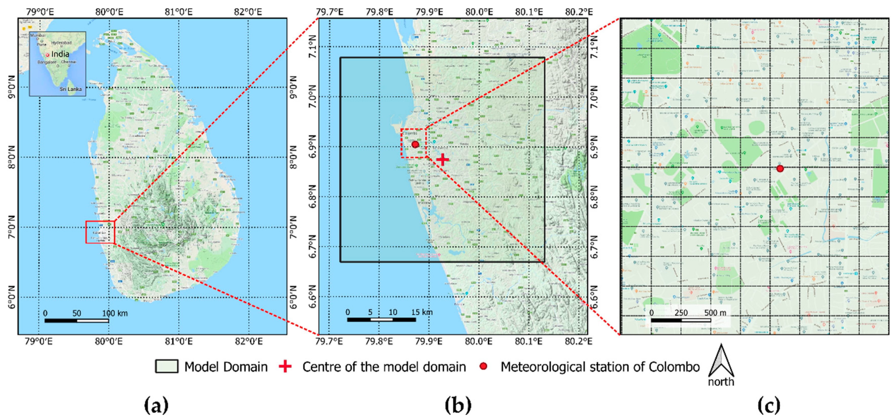
2.1. Study Area
2.2. UrbClim
2.3. Model Setup
2.4. Numerical Simulations
3. Results
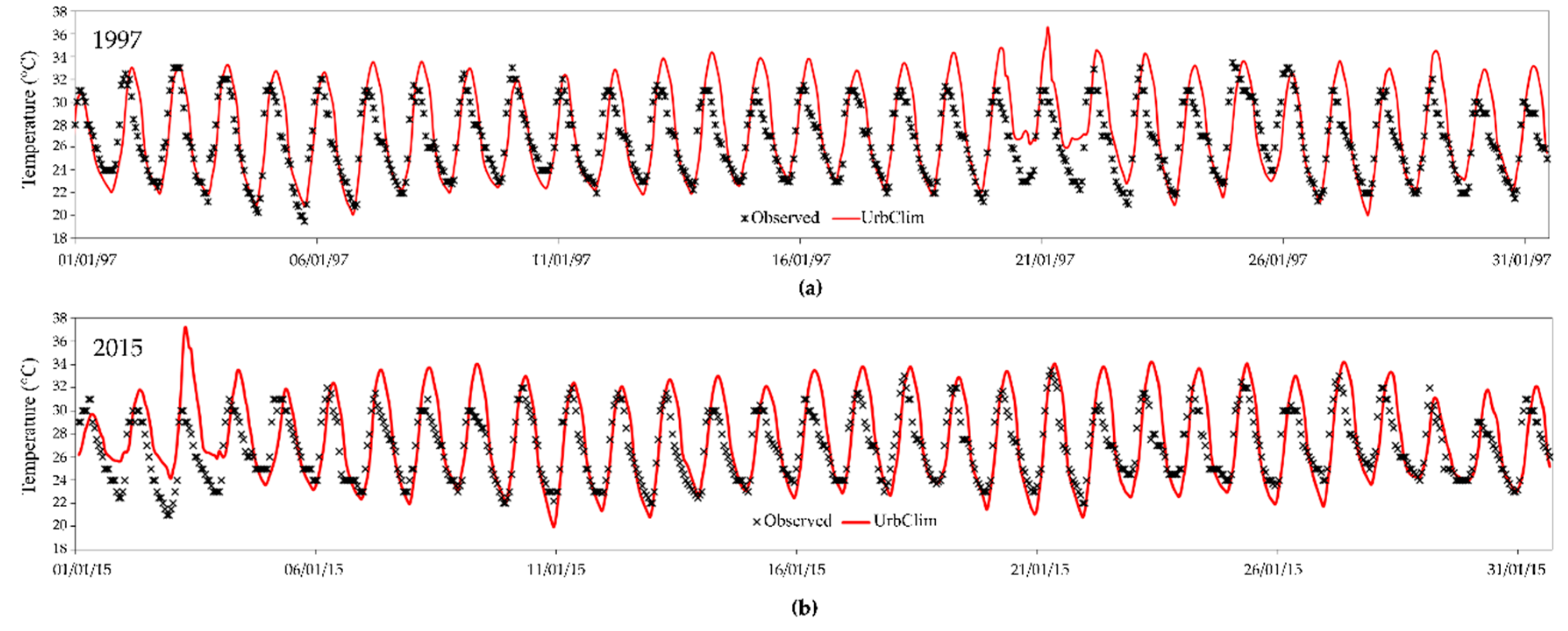
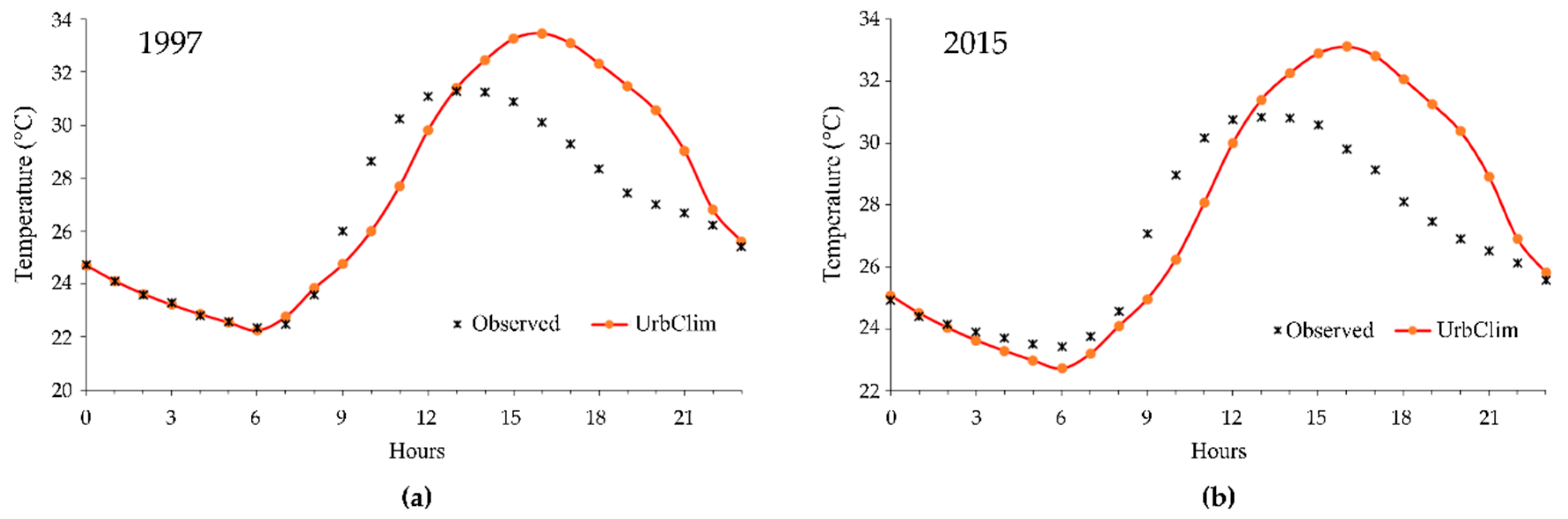
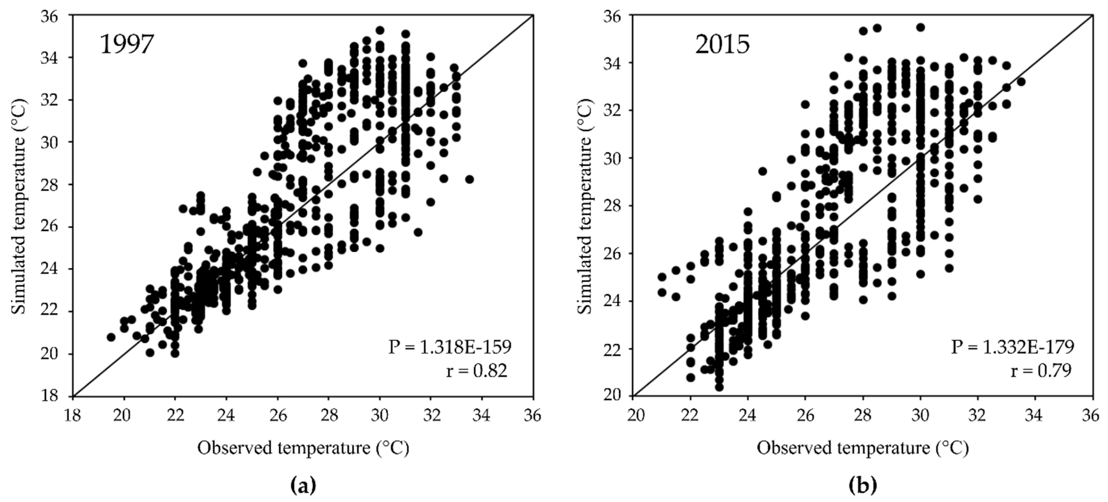
3.1. Model Validation
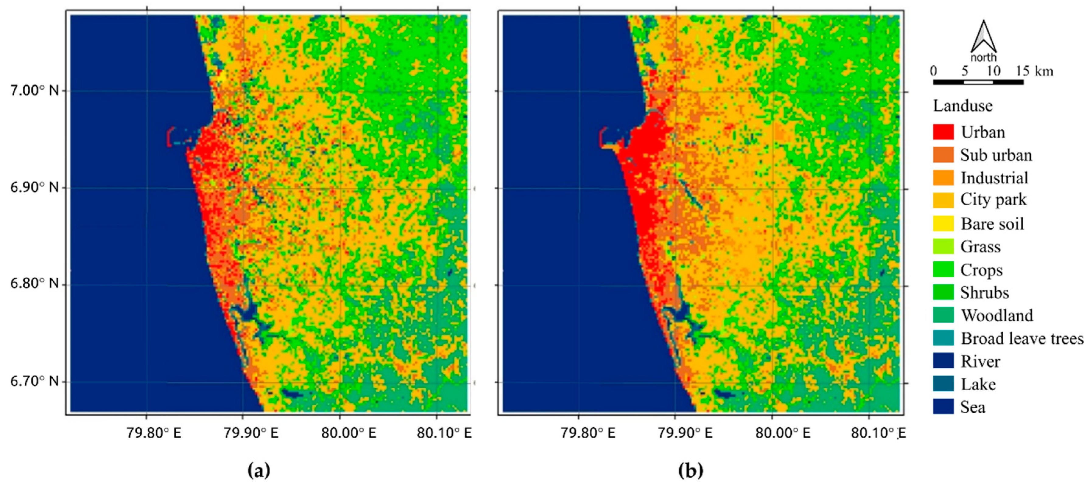
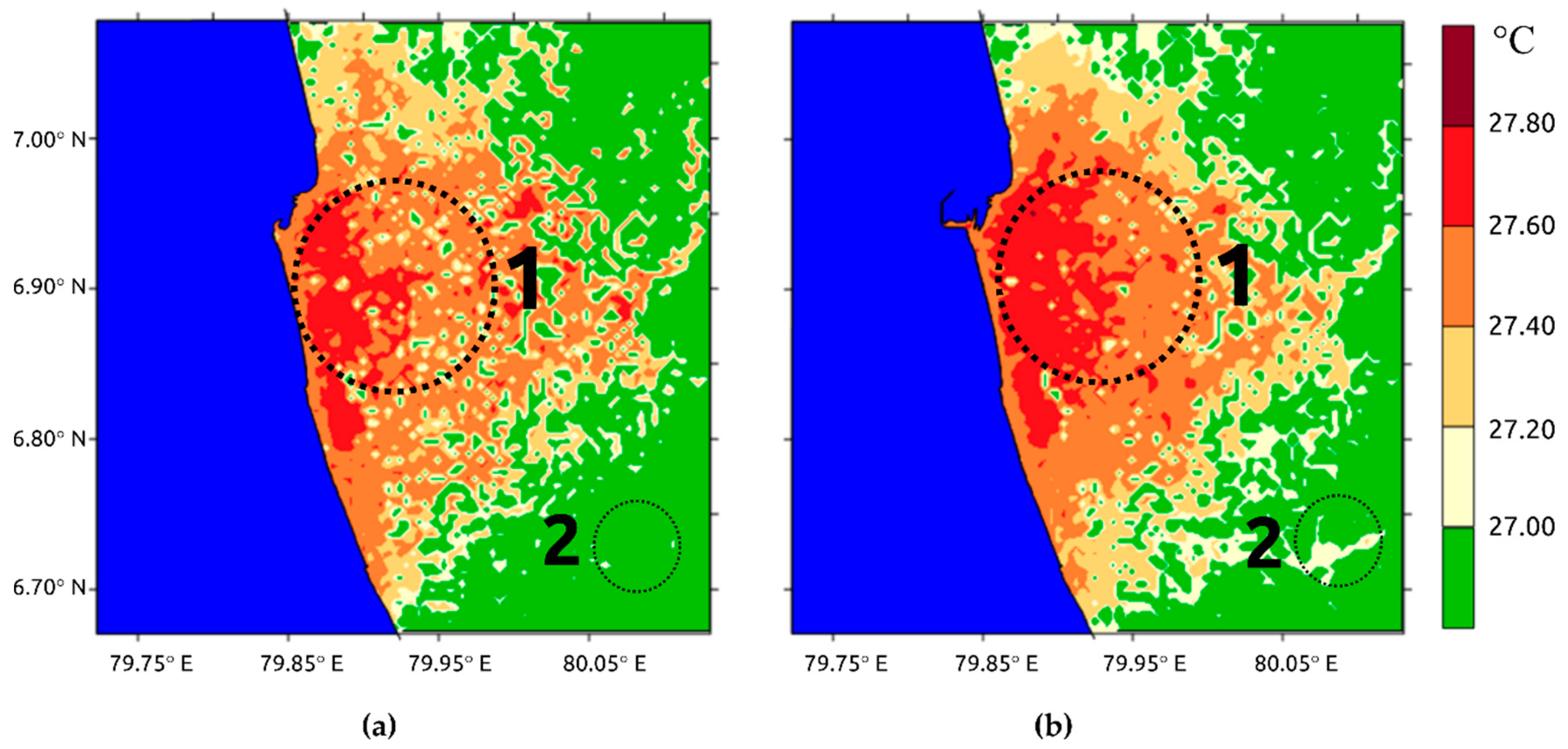
3.2. Impact of Land-Use Change on UHIs
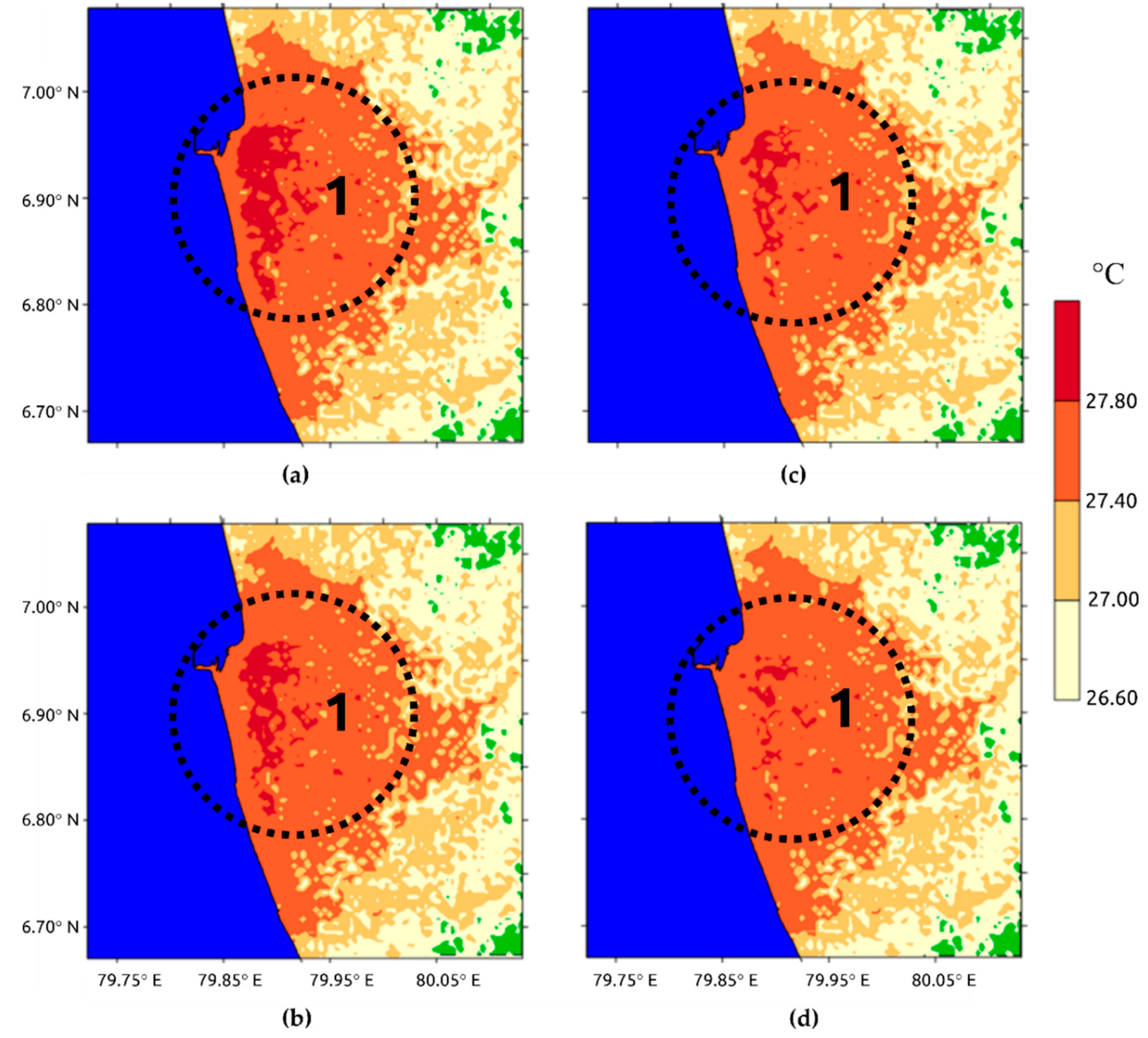
3.3. Greening Simulations
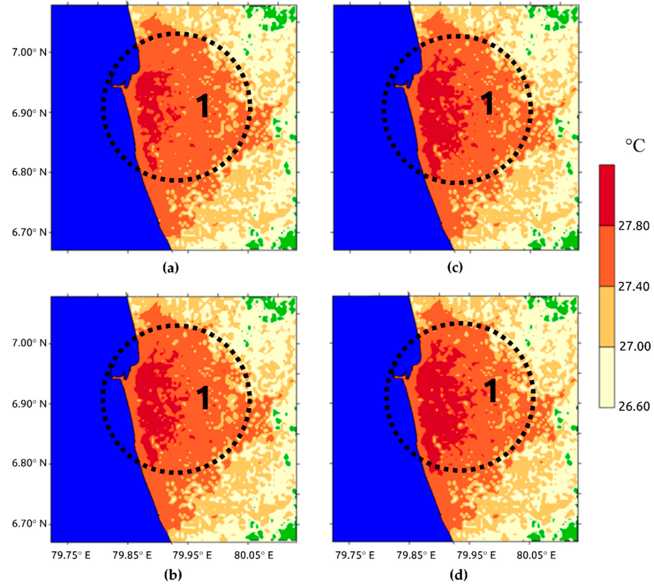
3.4. Urban Expansion Simulations
4. Discussion
5. Conclusions
Author Contributions
Funding
Acknowledgments
Conflicts of Interest
References
- Fu, P.; Weng, Q. Responses of urban heat island in Atlanta to different land-use scenarios. Theor. Appl. Climatol. 2017, 1–13. [Google Scholar] [CrossRef]
- Ahmed, S. Climate risks in megacities of the global south: Focus on Dhaka, Bangladesh. In The “State of DRR at the Local Level” A 2015 Report on the Patterns of Disaster Risk Reduction Actions at Local Level; UNISDR: Geneva, Switzerland, 2015; pp. 1–11. [Google Scholar]
- Doan, Q.-V.; Kusaka, H. Numerical study on regional climate change due to the rapid urbanization of greater Ho Chi Minh City’s metropolitan area over the past 20 years. Int. J. Climatol. 2016, 36, 3633–3650. [Google Scholar] [CrossRef]
- Uz Zaman Chaudhry, Q.; Rasul, G.; Kamal, A.; Ahmad Mangrio, M.; Mahmood, S. Technical Report on Karachi Heatwave June 2015; Government of Pakistan Ministry of Climate Change: Karachi, Pakistan, 2015.
- Tokairin, T.; Sofyan, A.; Kitada, T. Effect of land use changes on local meteorological conditions in Jakarta, Indonesia: Toward the evaluation of the thermal environment of megacities in Asia. Int. J. Climatol. 2010, 30, 1931–1941. [Google Scholar] [CrossRef]
- Vidanapathirana, M.; Perera, N.G.R.; Emmanuel, R. Microclimatic impacts of high-rise cluster developments in Colombo, Sri Lanka. In “Design that Cares—Inter Disciplinary Approach to Making Built Environments Efficient and Meaningful”: Proceedings of the 10th International Conference of Faculty of Architecture Research Unit (FARU); Rajapaksa, U., Ed.; University of Moratuwa: Moratuwa, Sri Lanka, 2017; pp. 1–12. [Google Scholar]
- Matsumoto, J.; Fujibe, F.; Takahashi, H. Urban climate in the Tokyo metropolitan area in Japan. J. Environ. Sci. 2017, 59, 54–62. [Google Scholar] [CrossRef] [PubMed]
- Steul, K.; Schade, M.; Heudorf, U. Mortality during heatwaves 2003–2015 in Frankfurt-Main – the 2003 heatwave and its implications. Int. J. Hyg. Environ. Health 2018, 221, 81–86. [Google Scholar] [CrossRef] [PubMed]
- Xu, Z.; Cheng, J.; Hu, W.; Tong, S. Heatwave and health events: A systematic evaluation of different temperature indicators, heatwave intensities and durations. Sci. Total Environ. 2018, 630, 679–689. [Google Scholar] [CrossRef] [PubMed]
- Kasai, M.; Okaze, T.; Mochida, A.; Hanaoka, K. Heatstroke risk predictions for current and near-future summers in Sendai, Japan, based on mesoscale WRF simulations. Sustainability 2017, 9, 1467. [Google Scholar] [CrossRef]
- Watts, N.; Amann, M.; Ayeb-Karlsson, S.; Belesova, K.; Bouley, T.; Boykoff, M.; Byass, P.; Cai, W.; Campbell-Lendrum, D.; Chambers, J.; et al. The Lancet Countdown on health and climate change: From 25 years of inaction to a global transformation for public health. Lancet 2017, 6736. [Google Scholar] [CrossRef]
- Hirano, Y.; Fujita, T. Evaluation of the impact of the urban heat island on residential and commercial energy consumption in Tokyo. Energy 2012, 37, 371–383. [Google Scholar] [CrossRef]
- Kolokotroni, M.; Ren, X.; Davies, M.; Mavrogianni, A. London’s urban heat island: Impact on current and future energy consumption in office buildings. Energy Build. 2012, 47, 302–311. [Google Scholar] [CrossRef]
- Bao, T.; Li, X.; Zhang, J.; Zhang, Y.; Tian, S. Assessing the distribution of urban green spaces and its anisotropic cooling distance on urban heat island pattern in Baotou, China. ISPRS Int. J. Geo-Inf. 2016, 5, 12. [Google Scholar] [CrossRef]
- Huong, H.T.L.; Pathirana, A. Urbanization and climate change impacts on future urban flooding in Can Tho city, Vietnam. Hydrol. Earth Syst. Sci. 2013, 17, 379–394. [Google Scholar] [CrossRef]
- Pachauri, R.K.; Reisinger, A. Contribution of Working Groups I, II and III to the Fourth Assessment Report of the Intergovernmental Panel on Climate Change; IPCC: Geneva, Switzerland, 2007. [Google Scholar]
- Zope, P.E.; Eldho, T.I.; Jothiprakash, V. Hydrological impacts of land use land cover change and detention basins on urban flood hazard: a case study of Poisar River basin, Mumbai, India. Nat. Hazards 2017, 1–17. [Google Scholar] [CrossRef]
- Lin, C.Y.; Chen, W.C.; Chang, P.L.; Sheng, Y.F. Impact of the urban heat island effect on precipitation over a complex geographic environment in northern Taiwan. J. Appl. Meteorol. Climatol. 2011, 50, 339–353. [Google Scholar] [CrossRef]
- Pathirana, A.; Denekew, H.B.; Veerbeek, W.; Zevenbergen, C.; Banda, A.T. Impact of urban growth-driven landuse change on microclimate and extreme precipitation—A sensitivity study. Atmos. Res. 2014, 138, 59–72. [Google Scholar] [CrossRef]
- Hidalgo, J.; Masson, V.; Baklanov, A.; Pigeon, G.; Gimeno, L. Advances in urban climate modeling. Ann. N. Y. Acad. Sci. 2008, 1146, 354–374. [Google Scholar] [CrossRef] [PubMed]
- Wallace, J.M.; Hobbs, P.V. Atmospheric Science, an Introductory Survey; Elsevier: Amsterdam, The Netherlands, 2006; Volume 7, ISBN 0-12-732951-X. [Google Scholar]
- U.S. Environmental Protection Agency. Reducing Urban Heat Islands: Compendium of Strategies Urban Heat Island Basics; U.S. Environmental Protection Agency: Washington, DC, USA, 2008.
- Brown, M.J.; Grimmond, S. Sky View Factor Measurements in Downtown Salt Lake City-Data Report for the DOE CBNP URBAN Experiment; Los Alamos National Laboratory: Los Alamos, NM, USA, 2001; Volume 836. [Google Scholar]
- Svensson, M.K. Sky view factor analysis – implications for urban air temperature differences. Meteorol. Appl. 2004, 11, 201–211. [Google Scholar] [CrossRef]
- Li, H.; Meier, F.; Lee, X.; Chakraborty, T.; Liu, J.; Schaap, M.; Sodoudi, S. Interaction between urban heat island and urban pollution island during summer in Berlin. Sci. Total Environ. 2018, 636, 818–828. [Google Scholar] [CrossRef] [PubMed]
- Taylor, L.; Hochuli, D.F. Defining greenspace: Multiple uses across multiple disciplines. Landsc. Urban Plan. 2017, 158, 25–38. [Google Scholar] [CrossRef]
- Rotterdam, C. Rotterdam Programme on Sustainability and Climate Change 2015-2018; City of Rotterdam: Rotterdam, The Netherlands, 2015. [Google Scholar]
- Bolund, P.; Hunhammar, S. Ecosystem services in urban areas. Ecol. Econ. 1999, 29, 293–301. [Google Scholar] [CrossRef]
- Charlesworth, S.M. A review of the adaptation and mitigation of global climate change using sustainable drainage in cities. J. Water Clim. Chang. 2010, 1, 165–180. [Google Scholar] [CrossRef]
- Forman, R.T.T. Landscape Mosaic: The Ecology of Landscape and Regions; Cambridge University Press: New York, NY, USA, 1995. [Google Scholar]
- Sun, R.; Chen, L. Effects of green space dynamics on urban heat islands: Mitigation and diversification. Ecosyst. Serv. 2017, 23, 38–46. [Google Scholar] [CrossRef]
- Tran, D.X.; Pla, F.; Latorre-Carmona, P.; Myint, S.W.; Caetano, M.; Kieu, H.V. Characterizing the relationship between land use land cover change and land surface temperature. ISPRS J. Photogramm. Remote Sens. 2017, 124, 119–132. [Google Scholar] [CrossRef]
- Zhou, W.; Huang, G.; Cadenasso, M.L. Does spatial configuration matter? Understanding the effects of land cover pattern on land surface temperature in urban landscapes. Landsc. Urban Plan. 2011, 102, 54–63. [Google Scholar] [CrossRef]
- Sodoudi, S.; Zhang, H.; Chi, X.; Müller, F.; Li, H. The influence of spatial configuration of green areas on microclimate and thermal comfort. Urban For. Urban Green. 2018, 34, 85–96. [Google Scholar] [CrossRef]
- Xiao, X.D.; Dong, L.; Yan, H.; Yang, N.; Xiong, Y. The influence of the spatial characteristics of urban green space on the urban heat island effect in Suzhou Industrial Park. Sustain. Cities Soc. 2018, 40, 428–439. [Google Scholar] [CrossRef]
- Connors, J.P.; Galletti, C.S.; Chow, W.T.L. Landscape configuration and urban heat island effects: Assessing the relationship between landscape characteristics and land surface temperature in Phoenix, Arizona. Landsc. Ecol. 2013, 28, 271–283. [Google Scholar] [CrossRef]
- Kikon, N.; Singh, P.; Singh, S.K.; Vyas, A. Assessment of urban heat islands (UHI) of Noida City, India using multi-temporal satellite data. Sustain. Cities Soc. 2016, 22, 19–28. [Google Scholar] [CrossRef]
- Lian, L.; Li, B.; Chen, Y.; Chu, C.; Qin, Y. Quantifying the effects of LUCCs on local temperatures, precipitation, and wind using the WRF model. Environ. Monit. Assess. 2017, 189. [Google Scholar] [CrossRef]
- Ramdhoni, S.; Rushayati, S.B. Open green space development priority based on distribution of air temperature change in capital city of Indonesia, Jakarta. Procedia Environ. Sci. 2016, 33, 204–213. [Google Scholar] [CrossRef]
- Ranagalage, M.; Estoque, R.C.; Murayama, Y. An urban heat island study of the Colombo Metropolitan Area, Sri Lanka, based on Landsat data (1997–2017). ISPRS Int. J. Geo-Inf. 2017, 6, 189. [Google Scholar] [CrossRef]
- Senanayake, I.P.; Welivitiya, W.D.D.P.; Nadeeka, P.M. Remote sensing based analysis of urban heat islands with vegetation cover in Colombo city, Sri Lanka using Landsat-7 ETM+ data. Urban Clim. 2013, 5, 19–35. [Google Scholar] [CrossRef]
- Kleerekoper, L.; Van Esch, M.; Salcedo, T.B. How to make a city climate-proof, addressing the urban heat island effect. Resour. Conserv. Recycl. 2012, 64, 30–38. [Google Scholar] [CrossRef]
- Neema, M.N.; Ohgai, A. Multitype green-space modeling for urban planning using GA and GIS. Environ. Plan. B Plan. Des. 2013, 40, 447–473. [Google Scholar] [CrossRef]
- Zhang, Y.; Murray, A.T.; Turner, B.L. Optimizing green space locations to reduce daytime and nighttime urban heat island effects in Phoenix, Arizona. Landsc. Urban Plan. 2017, 165, 162–171. [Google Scholar] [CrossRef]
- Kusaka, H.; Suzuki-Parker, A.; Aoyagi, T.; Adachi, S.A.; Yamagata, Y. Assessment of RCM and urban scenarios uncertainties in the climate projections for August in the 2050s in Tokyo. Clim. Chang. 2016, 137, 427–438. [Google Scholar] [CrossRef]
- Wang, J.; Huang, B.; Fu, D.; Atkinson, P.M.; Zhang, X. Response of urban heat island to future urban expansion over the Beijing-Tianjin-Hebei metropolitan area. Appl. Geogr. 2016, 70, 26–36. [Google Scholar] [CrossRef]
- Kubota, T.; Lee, H.S.; Trihamdani, A.R.; Phuong, T.T.T.; Tanaka, T.; Matsuo, K. Impacts of land use changes from the Hanoi Master Plan 2030 on urban heat islands: Part 1. Cooling effects of proposed green strategies. Sustain. Cities Soc. 2017, 32, 295–317. [Google Scholar] [CrossRef]
- Lee, H.S.; Trihamdani, A.R.; Kubota, T.; Iizuka, S.; Phuong, T.T.T. Impacts of land use changes from the Hanoi Master Plan 2030 on urban heat islands: Part 2. Influence of global warming. Sustain. Cities Soc. 2017, 31, 95–108. [Google Scholar] [CrossRef]
- Doan, V.Q. Projections of urban climate in the 2050s in a fast-growing city in Southeast Asia: The greater Ho Chi Minh City metropolitan area, Vietnam. Int. J. Climatol. 2018, 1–17. [Google Scholar] [CrossRef]
- Li, H.; Zhou, Y.; Li, X.; Meng, L.; Wang, X.; Wu, S.; Sodoudi, S. A new method to quantify surface urban heat island intensity. Sci. Total Environ. 2018, 624, 262–272. [Google Scholar] [CrossRef]
- Oke, T.R.; Mills, G.; Christen, A.; Voogt, J.A. Urban Climates; Cambridge University Press: Cambridge, UK, 2017; ISBN 9781139016476. [Google Scholar]
- Voogt, J.A.; Oke, T.R. Thermal remote sensing of urban climates. Remote Sens. Environ. 2003, 86, 370–384. [Google Scholar] [CrossRef]
- Weng, Q. Thermal infrared remote sensing for urban climate and environmental studies: Methods, applications, and trends. ISPRS J. Photogramm. Remote Sens. 2009, 64, 335–344. [Google Scholar] [CrossRef]
- De Ridder, K.; Lauwaet, D.; Maiheu, B. UrbClim—A fast urban boundary layer climate model. Urban Clim. 2015, 12, 21–48. [Google Scholar] [CrossRef]
- García-Díez, M.; Lauwaet, D.; Hooyberghs, H.; Ballester, J.; De Ridder, K.; Rodó, X. Advantages of using a fast urban canopy model as compared to a full mesoscale model to simulate the urban heat island of Barcelona. Geosci. Model Dev. Discuss. 2016, 1–17. [Google Scholar] [CrossRef]
- Lauwaet, D.; De Nijs, T.; Liekens, I.; Hooyberghs, H.; Verachtert, E.; Lefebvre, W.; De Ridder, K.; Remme, R.; Broekx, S. A new method for fine-scale assessments of the average urban heat island over large areas and the effectiveness of nature-based solutions. One Ecosyst. 2018, 3, e24880. [Google Scholar] [CrossRef]
- Skamarock, W.C.; Klemp, J.B.; Dudhi, J.; Gill, D.O.; Barker, D.M.; Duda, M.G.; Huang, X.-Y.; Wang, W.; Powers, J.G. A description of the advanced research WRF version 3. Tech. Rep. 2008, 113. [Google Scholar] [CrossRef]
- Lazarova, L.; Kusaka, H. Study on the urban heat island in Sofia City: Numerical simulations with potential natural vegetation and present land use data. Sustain. Cities Soc. 2018, 40, 110–125. [Google Scholar] [CrossRef]
- Li, H.; Zhou, Y.; Wang, X.; Zhou, X.; Zhang, H.; Sodoudi, S. Quantifying urban heat island intensity and its physical mechanism using WRF/UCM. Sci. Total Environ. 2019, 650, 3110–3119. [Google Scholar] [CrossRef]
- Trusilova, K.; Früh, B.; Brienen, S.; Walter, A.; Masson, V.; Pigeon, G.; Becker, P. Implementation of an urban parameterization scheme into the regional climate model COSMO-CLM. J. Appl. Meteorol. Climatol. 2013, 52, 2296–2311. [Google Scholar] [CrossRef]
- Kuchelmeister, G. Urban Forestry in the Asia-Pacific Region: Status and Prospects; Asia-Pacific Forestry Sector Outlook Study Working Paper; FAO Regional Office for Asia and the Pacific: Bangkok, Thailand, 1998. [Google Scholar]
- Senanayake, I.P.; Welivitiya, W.D.D.P.; Nadeeka, P.M. Urban green spaces analysis for development planning in Colombo, Sri Lanka, utilizing THEOS satellite imagery – A remote sensing and GIS approach. Urban For. Urban Green. 2013, 12, 307–314. [Google Scholar] [CrossRef]
- Perera, N.G.R. Climate-Sensitive Urban Public Space: A Sustainable Approach to Urban Heat Island Mitigation in Colombo, Sri Lanka; University of Moratuwa: Moratuwa, Sri Lanka, 2015. [Google Scholar]
- De Ridder, K.; Schayes, G. The IAGL land surface model. J. Appl. Meteorol. 1997, 36, 167–182. [Google Scholar] [CrossRef]
- Sharma, R.; Hooyberghs, H.; Lauwaet, D.; Ridder, K. Urban heat island and future climate change—Implications for Delhi’s heat. J. Urban Heal. 2018. [Google Scholar] [CrossRef] [PubMed]
- Bechtel, B.; Alexander, P.; Böhner, J.; Ching, J.; Conrad, O.; Feddema, J.; Mills, G.; See, L.; Stewart, I. Mapping local climate zones for a worldwide database of the form and function of cities. ISPRS Int. J. Geo-Inf. 2015, 4, 199–219. [Google Scholar] [CrossRef]
- Stewart, I.D.; Oke, T.R. Local climate zones for urban temperature studies. Bull. Am. Meteorol. Soc. 2012, 93, 1879–1900. [Google Scholar] [CrossRef]
- Perera, N.G.R.; Emmanuel, R. A “Local Climate Zone” based approach to urban planning in Colombo, Sri Lanka. Urban Clim. 2018, 23, 188–203. [Google Scholar] [CrossRef]
- Ren, C.; Fung, J.C.-H.; Tse, J.W.P.; Wang, R.; Wong, M.M.F.; Xu, Y. Implementing WUDAPT product into urban development impact analysis by using WRF simulation result—A case study of the Pearl River Delta Region (1980–2010). In Proceedings of the 9th American Meteorological Society Annual Meeting 2017 (AMS2017), Seattle, WA, USA, 22–26 January 2017; pp. 22–26. [Google Scholar]
- Best, M.J.; Grimmond, C.S.B. Analysis of the seasonal cycle within the first international urban land-surface model comparison. Bound.-Layer Meteorol. 2013, 146, 421–446. [Google Scholar] [CrossRef]
- Chai, T.; Draxler, R.R. Root mean square error (RMSE) or mean absolute error (MAE)? -Arguments against avoiding RMSE in the literature. Geosci. Model Dev. 2014, 7, 1247–1250. [Google Scholar] [CrossRef]
- Emery, C.; Tai, E.; Yarwood, G. Enhanced meteorological modeling and performance evaluation for two texas ozone episodes. Env. Int. Corp. 2001, 235. [Google Scholar]
- Oke, T.R. The Energetic Basis of The Urban Heat Island. Q. J. R. Meteorol. Soc. 1982, 108, 1–24. [Google Scholar] [CrossRef]
- Gunawardena, K.R.; Wells, M.J.; Kershaw, T. Utilising green and bluespace to mitigate urban heat island intensity. Sci. Total Environ. 2017, 584–585, 1040–1055. [Google Scholar] [CrossRef]
- Derkzen, M.L.; van Teeffelen, A.J.A.; Verburg, P.H. Quantifying urban ecosystem services based on high-resolution data of urban green space: An assessment for Rotterdam, the Netherlands. J. Appl. Ecol. 2015, 52, 1020–1032. [Google Scholar] [CrossRef]
- Gkatsopoulos, P. A methodology for calculating cooling from vegetation evapotranspiration for use in urban space microclimate simulations. Procedia Environ. Sci. 2017, 38, 477–484. [Google Scholar] [CrossRef]
- Li, H.; Wolter, M.; Wang, X.; Sodoudi, S. Impact of land cover data on the simulation of urban heat island for Berlin using WRF coupled with bulk approach of Noah-LSM. Theor. Appl. Climatol. 2017, 1–15. [Google Scholar] [CrossRef]
- Oke, T.R. The urban energy balance. Prog. Phys. Geogr. 1988, 12, 471–508. [Google Scholar] [CrossRef]
- Amorim, M.C.d.C.T.; Dubreuil, V. Intensity of urban heat islands in tropical and temperate climates. Climate 2017, 5, 91. [Google Scholar] [CrossRef]
- Gharesifard, M.; Wehn, U.; van der Zaag, P. Towards benchmarking citizen observatories: Features and functioning of online amateur weather networks. J. Environ. Manag. 2017, 193, 381–393. [Google Scholar] [CrossRef] [PubMed]


| Land-Use Classes | Land-Use Change (%) |
|---|---|
| Urban | 50.90 |
| Suburban | −15.50 |
| Industrial | 32.39 |
| City Park | 2.01 |
| Green Areas (Grass, Crops, Shrubs, Woodland, Broadleaf Trees) | −8.94 |
| Open Water (River, Sea, Lake) | −8.97 |
| Simulation | Average Temperature in Urban Areas (°C) | Average Daytime UHI (°C) | Average Nighttime UHI (°C) | The Area Experience More Than 27.8 °C as Avg. Temperature (km2) | Area Reduction (km2) |
|---|---|---|---|---|---|
| Existing situation | 27.75 | 0.26 | 1.41 | 67.12 | |
| Scenario 1 | 27.72 | 0.25 | 1.33 | 49.50 | 17.62 |
| Scenario 2 | 27.70 | 0.24 | 1.28 | 35.87 | 31.25 |
| Scenario 3 | 27.67 | 0.22 | 1.25 | 23.81 | 43.31 |
| Simulation | Average Temperature in Urban Areas (°C) | Average Daytime UHI (°C) | Average Nighttime UHI (°C) | The Area with Avg. Temperature More Than 27.8 °C (km2) | Increased Areas (km2) |
|---|---|---|---|---|---|
| Existing situation | 27.75 | 0.26 | 1.41 | 67.12 | |
| Scenario 4 | 27.76 | 0.22 | 1.42 | 102.75 | 35.63 |
| Scenario 5 | 27.77 | 0.22 | 1.42 | 119.13 | 52.01 |
| Scenario 6 | 27.78 | 0.22 | 1.44 | 142.31 | 75.19 |
© 2019 by the authors. Licensee MDPI, Basel, Switzerland. This article is an open access article distributed under the terms and conditions of the Creative Commons Attribution (CC BY) license (http://creativecommons.org/licenses/by/4.0/).
Share and Cite
Maheng, D.; Ducton, I.; Lauwaet, D.; Zevenbergen, C.; Pathirana, A. The Sensitivity of Urban Heat Island to Urban Green Space—A Model-Based Study of City of Colombo, Sri Lanka. Atmosphere 2019, 10, 151. https://doi.org/10.3390/atmos10030151
Maheng D, Ducton I, Lauwaet D, Zevenbergen C, Pathirana A. The Sensitivity of Urban Heat Island to Urban Green Space—A Model-Based Study of City of Colombo, Sri Lanka. Atmosphere. 2019; 10(3):151. https://doi.org/10.3390/atmos10030151
Chicago/Turabian StyleMaheng, Dikman, Ishara Ducton, Dirk Lauwaet, Chris Zevenbergen, and Assela Pathirana. 2019. "The Sensitivity of Urban Heat Island to Urban Green Space—A Model-Based Study of City of Colombo, Sri Lanka" Atmosphere 10, no. 3: 151. https://doi.org/10.3390/atmos10030151
APA StyleMaheng, D., Ducton, I., Lauwaet, D., Zevenbergen, C., & Pathirana, A. (2019). The Sensitivity of Urban Heat Island to Urban Green Space—A Model-Based Study of City of Colombo, Sri Lanka. Atmosphere, 10(3), 151. https://doi.org/10.3390/atmos10030151