The Causes of “Vulnerable Regions” to Air Pollution in Winter in the Beijing-Tianjin-Hebei Region: A Topographic–Meteorological Impact Model Based on Adaptive Emission Constraint Technique

Abstract

The Beijing-Tianjin-Hebei (BTH) region, with its complex terrain, has serious issues with air pollution. The northern and western parts of the BTH region are surrounded by the Yan Mountains and Loess Plateau (LP), and the south-central part of that region is a large open plain. Such special geographic configuration is prone to result in a concentrated pollution belt along the north-to-south direction on the eastern margin of the plateau, in addition to the influence of pollutant-emission sources and population distribution. In this study, based on an original adaptive nudging constraint method, we quantitatively analyzed the differences in the influence of emission sources under different dynamic and thermal conditions in the BTH region, which is impacted by a special large-scale leeward slope terrain. The mechanism of air pollution vulnerability and the comprehensive effects of terrain–meteorological conditions on air pollution in the BTH region were also discussed. The results indicated that the atmospheric diffusion conditions on the eastern side of the plateau were poor, and a sub-synoptic-scale “vortex sequence”, which was composed of a series of linked vortices, was identified. The corresponding atmospheric pollution convergence line stretched from Beijing to Hebei to Northern Henan in the lower atmosphere. On the eastern edge of the plateau, a “warm cover” formed by a temperature anomaly and a downdraft impeded the vertical diffusion of pollutants. Therefore, pollutants tended to converge at the eastern edge of the plateau, and the pollution belts would move longitudinally north and south along the topography of the eastern slope when south-westerly and north-easterly winds alternated. The movement generated a “train” of pollutants that were transported on the eastern edge of the plateau, which then caused air pollution to persist there. Such terrain–meteorological conditions amplified the effects of emissions by an average of 50% to 150% in the region, leading the eastern side of the LP to become a “naturally vulnerable region” to haze pollution.

1. Introduction

The Beijing-Tianjin-Hebei (BTH) region has been suffering from the most severe haze in China [1,2,3]. Air pollution is closely related to the population density, industrial development, and the traffic intensity. Particulate matter, such as PM_2.5, is the major pollutant of winter haze in the BTH region [4], and it has a negative impact on ambient air quality and human health [5,6,7]. In 2013, the Chinese government established the “Action Plan for Air Pollution Prevention and Control”. Since the implementation of this measure, pollution control has been moderately successful [8]. The monitoring results of the ozone monitoring instrument (OMI) indicated that the amount of NO_X emissions in many cities in China has decreased by an average of 21% between 2005 and 2015 [9]. From 2012 to 2015, SO₂ in the North China Plain was reduced by 50% [10]. Although the total discharge of pollutants has decreased year by year, haze pollution events still occur occasionally [11,12]. In December 2016, five consecutive haze events occurred in the BTH region, with the most severe event occurring between 29 December 2016 and 7 January 2017. This haze event was of a long duration (10 days) and had a wide-ranging impact, accompanied by an explosive growth of PM_2.5 concentrations. The maximum hourly PM_2.5 concentration in Beijing exceeded 500 μg·m⁻³ [13]. Although the intensity of pollution control in the BTH region is unprecedented, the air quality of Baoding, Shijiazhuang, Xingtai, and Handan in the region have still ranked among the last five in China in 2016 and 2017 (Chinese Environmental Status Bulletin), which indicates that weather systems and meteorological factors also play a crucial role in the temporal and spatial evolution of haze pollution, in addition to the pollutant emissions.

Different haze pollution characteristics can be observed under different meteorological conditions and in different regions. Moreover, some regions are more susceptible to haze pollution under certain special meteorological conditions [14]. Atmospheric circulation, temperature stratification, boundary layer evolution, and air humidity can have a critical effect on the formation of pollution [15,16,17,18]. When cold air advection is weak, and there are subsidence and stable atmospheric stratification, a stagnant zone can be generated in the lower atmosphere, in which air pollutants are likely to accumulate [19]. Wu et al. [20] found that the concentration of SO₂ and NO₂ along the Taihang Mountain region is influenced by the southerly pollution transport, which was 1–2 times higher than that in the northerly wind. Zhang et al. [21] proposed that the contribution of meteorological factors to the variance of the daily fog and haze evolution reaches 0.68. 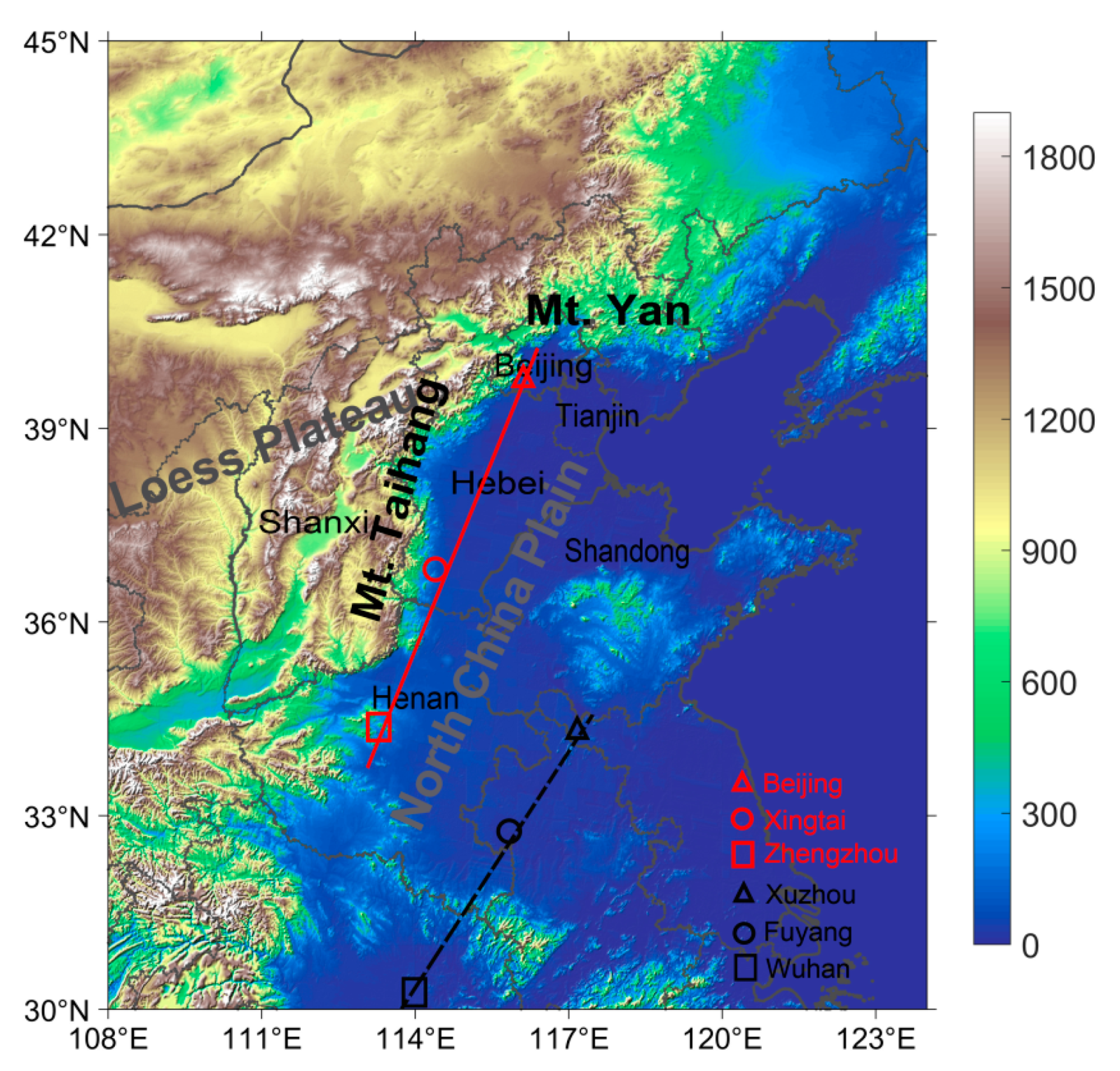Local circulation affected by terrain plays an important role under the force of weak large-scale meteorological conditions [22]. The terrain of the BTH region is complex, with the surrounding mountains (Yan Mountains to the north, Taihang Mountain to the west) and the coast to the east. The elevation differences between the mountainous regions and the plain in the BTH region can be as much as 1000 m (Figure 1). The mountains block the transport of contaminants and alter the local circulation patterns, resulting in thermal and dynamic structures that are not conducive to pollutant diffusion [13,23,24,25,26]. Through observations of the vertical temperature in the Gore River Valley of Colorado, Whiteman and Mckee [27] found that the inversion in the valley at night fell into the valley after sunrise, which is a common feature in the mountain regions. Guniya et al. [28] found that foehn processes substantially increase the air pollution level in the mountain countries. Xu et al. [29] found that there is an obvious wind convergence line downstream of the eastern margin of the Loess Plateau (hereafter referred to as the EMLP) when heavily polluted weather events occur in the BTH region. However, previous studies on haze pollution in the BTH region have focused on the statistical characteristics of pollution distribution and the weather conditions of haze events. We define the “vulnerable region” of air pollution as the highly concentrated band-shaped areas along the EMLP, which are caused by the combination of topography and meteorology, in addition to sources of pollutant emission and distribution of population. The impacts of different weather systems on the effects of emission sources, the synergistic effects of winter-dominated winds and large plateaus, the origin of the north–south pollution belt transport channel, and the causes of unique pollution regions (e.g., “vulnerable regions” to air pollution) are still not well understood. If the synergistic effect of the plateau terrain and the weather system on the spatial distribution of haze is recognized, the causes of the “vulnerable region” to pollution and its meteorological impact can be determined. As a result, urban planners can appropriately adjust the industrial layout and enact city development plans.

This study applied the adaptive emission constraint technique with the nudging method, which is based on the iterative solution to the meteorological–chemical transport model, to constrain daily emissions by considering the impacts of meteorological conditions [30] (the emissions with the consideration of meteorological conditions will be referred as EMC hereafter) from 1 December 2016 to 31 January 2017. The constraint method uses the Community Multiscale Air Quality (CMAQ) model [31,32] as an iterative inversion kernel. In the pollutant concentration prediction equation, the “relaxation adjustment term” of the emission source is included to reduce the error between the simulation result and the observation. Because this method excludes the long-distance transportation of pollutants, it effectively reflects the combined effects of regional meteorological conditions and emissions. By analyzing the correlations between EMC and the daily meteorological factors, as well as the thermal and dynamic parameters, we examined the impacts of different dominant wind fields on the distribution of pollution and the mechanism of the centralization of pollutants along the EMLP. The purpose of this study is to clarify the topographic–meteorological causes of the vulnerability in the BTH region under the influences of the LP and mountain topography.

2. Materials and Methods

In this study, we constrained the daily influence of the sources under different meteorological conditions (EMC) (from 1 December 2016 to 31 January 2017) by using the adaptive “nudging” emission constraint method (see Section 2.2.1) with the Weather Research and Forecasting—Community Multiscale Air Quality (WRF-CMAQ) model and the NO₂ mass concentration observations. The causes for the vulnerability of BTH region to air pollution in winter under the influence of large-scale terrain were quantitatively analyzed. To analyze the distribution characteristics of pollutants in the BTH region, the PM_2.5 and NO₂ mass concentration observation data were used. Wind fields reanalysis data were used to calculate the atmospheric ventilation and to analyze the spatial patterns of atmospheric diffusion conditions in Eastern China. The influences of plateau on the vertical diffusion of pollutants were studied by using the L-band sounding temperature and the NO₂ mass concentration observation data.

2.1. Data

In this study, the 0.25° wind fields reanalysis data (from 1 December 2016 to 31 January 2017) from the National Center for Environmental Prediction (NCEP) (http://nomads.ncep.noaa.gov/) were used to calculate the atmospheric ventilation and to analyze the physical mechanism of the effects of meteorological conditions on the changes of pollutant concentration (see Section 3.1, Section 3.3, and Section 3.5). L-band sounding system can detect meteorological-element profiles, e.g., the vertical profile of air pressure, temperature, humidity, wind direction, and wind speed. The temperature sounding data used in this study were from the China Meteorological Administration Sounding Observation Network, with a sampling frequency of 1.2 s and vertical resolution of 8 m. This study employed the L-band sounding temperature for the winters of 2014, 2015, and 2016, to analyze the influence of plateau on the vertical diffusion of pollutants (see Section 3.4). We selected representative stations both near to (Beijing, Xingtai, and Zhengzhou) and far from (Xuzhou, Fuyang, and Wuhan) the plateau (Figure 1), to investigate the effects of the plateau on the vertical diffusion of pollutants.

The PM_2.5, NO₂, and SO₂ mass concentration data were obtained from the operational surface observations of the Ministry of Ecology and Environment of China. PM_2.5 and NO₂ concentration observations were used to analyze the distribution characteristics of pollutants in the BTH region in winter (see Section 3.1). NO₂ mass concentrations were used to retrieve the EMC (see Section 2.2) and to analyze the physical mechanism of the impact of terrain on meteorological conditions (see Section 3.3, Section 3.4, Section 3.5). In this study, we used the daily mean value of ground–atmospheric composition observation data. The data contained about 1400 atmospheric-composition monitoring stations in the central and eastern regions of China, of which about 220 were in the BTH region.

2.2. Emission Constraint Method and Evaluation

2.2.1. Adaptive “Nudging” Emission Constraint Method

This adaptive “nudging” emission constraint method uses the CMAQ air quality model [31,32] as an iterative constraint kernel. The “relaxation adjustment term” of the emission source is added to the pollutant prediction equation to approximate the simulated and observed concentration, thereby determining the influence of the sources under different meteorological conditions (EMC). Therefore, EMC includes the effects of pollution emissions and changes in meteorological conditions.

For the concentration of a certain air pollutant, $P$, its Newtonian relaxation item can be expressed as follows, according to Xu et al. (2008) [30]:

$$\frac{\partial P_n}{\partial t}=F\left(P_n,x,t\right)+N\left(P_n,P^{*},Q_n\right),$$

(1)

where F represents the forcing function array, N is the nudging item, x denotes spatial dimensions, t is time, n is the number of iterations during the nudging process, $P^{*}$ is the on-spot observed concentration, and $Q_n$ is the estimated emission value after n iterations.

For pollutants, m, the emission intensity after iteration n + 1 ($Q_{1n+1},Q_{2n+1},\dots ,Q_{mn+1}$) can be calculated by using the following nudging equation:

$$\left(\begin{array}{c}\begin{array}{c}\begin{array}{c}{Q}_{1n+1}\\ Q_{2n+1}\end{array}\\ ⋮\end{array}\\ Q_{mn+1}\end{array}\right)=\left(\begin{array}{c}\begin{array}{c}\begin{array}{c}{Q}_{1n}\\ Q_{2n}\end{array}\\ ⋮\end{array}\\ Q_{mn}\end{array}\right)\left[\begin{array}{c}\begin{array}{c}\frac{P_1^{*}-{\beta }_1\left(P_{1n}-P_{1n-1}\right)}{P_{1n}}\\ \frac{P_2^{*}-{\beta }_2\left(P_{2n}-P_{2n-1}\right)}{P_{2n}}\\ ⋮\end{array}\\ \frac{P_m^{*}-{\beta }_m\left(P_{mn}-P_{mn-1}\right)}{P_{mn}}\end{array}\right]n=1,2,3,\cdots ,$$

(2)

where ${\beta }_n$ is the empirical nudging coefficient, which takes positive values when $P_m^{*}>P_{mn}$ and negative values when $P_m^{*}<P_{mn}$.

The emission intensities are determined as follows: (1) Input the initial emission source, $Q_{m1}$, into the CMAQ air-quality model, and simulate the first guess field, $P_{m1}$, of the mass concentration for species m. (2) Combine P_m1 with the observed concentration, $P_m^{*}$, to estimate the value of the emission source $Q_{m2}$. (3) Input $Q_{m2}$ into the CMAQ model to simulate the new concentration field, $P_{m2}$, and then iterate the above computational procedures. When $\Delta P_m=P_m^{*}-P_{mn}\approx 0$, the computed emission source intensity, $Q_{mn}$, is the final constrained emission source.

This work used the surface measurements of NO₂ from 1 December 2016 to 31 January 2017 and applied the nudging adaptive algorithm based on WRF-CMAQ model, to constrain the EMC. Due to the short life cycle of gaseous pollutants (e.g., NO₂; Seinfeld and Pandis, 2016) [33], which excludes the effects of long-distance transport in the atmosphere (e.g., PM_2.5), the calculated EMC of NO₂ can reveal the integrated influences of regional meteorological conditions and emissions. The results of the two-month EMC were averaged to represent emission intensity of the winter of 2016 (hereafter referred to as WINEMIS).

2.2.2. Numerical Model Setting for Source Constraining

We used the offline coupled systems WRFv3.5.1 and CMAQv4.7.1 to conduct the inverse modeling. In this study, the WRF model was used to simulate the meteorological field, and the simulation outputs were used to drive the air-quality mode CMAQ. The daily EMC in Central and Eastern China, from 1 December 2016 to 31 January 2017, were retrieved by using the source constraining method based on the WRF-CMAQ model and the daily average NO₂ concentration observations from about 1400 observation stations in Central and Eastern China (of which about 220 are in the BTH region). The NO₂ daily average concentration observations were interpolated to match the model grid.

The model setup included two domains with the horizontal resolutions of the outer and inner domains were 69 km and 23 km, respectively. The inner domain covered the Central–Eastern China region, and the grid center was located at 39° N, 107.6° E. The physical parameterization schemes employed in this study included the Kain–Fritsch cumulus schemes [34], the ACM2 boundary-layer scheme [35], the WSM6 microphysics scheme [36], and the RRTM longwave and Dudhia shortwave radiation schemes [37]. The Noah scheme was selected for the surface process [38]. The 6-hourly 0.5° Global Forecast System data produced by the National Centers for Environmental Prediction (GFS/NCEP; http://nomads.ncep.noaa.gov/) were used to provide the initial and lateral boundary conditions. We adopted a single domain in the CMAQ model. The outputs of the inner domain of the WRF model were served as the successive meteorological inputs to the CMAQ model. The Yamo scheme [39] was used to calculate the horizontal advection and the vertical convection. The ACM2 scheme was used as the solution to vertical diffusion [35]. The carbon bond mechanism (CB05CL-AE5-AQ) was selected for chemical reaction simulations, with the solution generated by an Euler backward iterative (EBI) algorithm [40]. The Multi-Resolution Emissions Inventory for China (MEIC) inventory data developed by Tsinghua University (http://www.meicmodel.org) for December 2012 was adopted as the initial emission source. The Sparse Matrix Operator Kernel Emissions (SMOKE) model [41] was applied to perform spatiotemporal distribution analyses, with the horizontal resolution of the gridded emissions being 23 km × 23 km with 16 vertical layers.

2.2.3. Reliability of the EMC

Cheng et al. [30], Meng et al. [42], and Xu et al. [43] have conducted source constraint studies in different regions of China and have shown that the EMC are reliable in terms of spatial distribution and magnitude. Therefore, this method can be served as an effective tool for controlling the haze and air pollution in various seasons.

By examining the convergence of a multiday mean EMC, it was found that the correlation coefficient between the 16-day average and the 62-day average reached 0.95 or higher. The EMC of the 16-day average from 8 December to 22 December 2016 were employed to simulate a heavy pollution event in the BTH region between 29 December 2016 and 7 January 2017. The simulation results were compared to the observed data and the simulation results using the MEIC inventory. The scatterplots show that the correlation coefficient between the simulated and observed NO₂ increases from 0.77 (from the M2012 simulations) to 0.85 (from the constrained emission simulations) (Figure 2). The simulation results using the EMC significantly improved the simulation results, which is consistent with the results of Meng et al. (2018) [44], demonstrating the reliability of the constraint method.

2.3. Atmospheric Ventilation

The height of the atmospheric mixing layer and the velocity of the wind in the mixing layer reflect the ability of the atmospheric process to diffuse pollutants. When the height of the mixing layer is low and the horizontal wind speed is small, the diffusion and dilution of the pollutants will decrease. Xu and Zhu [45] proposed the use of meteorological data to calculate the parameter $V_s$, which characterizes the state of atmospheric motion in the boundary layer. They used conventional meteorological observation data to study the distribution of ventilation volume in Mainland China. In this study, we calculated the atmospheric ventilation in Central and Eastern China by using 0.25° wind fields reanalysis data, and we analyzed the spatial distribution of the atmospheric diffusion conditions to understand the background information of the weak wind region under the influence of topographic–meteorological conditions (see Section 3.2). The calculation formula for ventilation volume $V_s$ is as follows:

$$V_s=\underset{0}{\overset{H}{{\displaystyle \int }}}U\left(z\right)dz$$

(3)

where $V_s$ is in m²·s⁻¹, H is the height of the mixed layer, and $U\left(z\right)=u^2+v^2$ is the wind-speed variation, with height in the mixed layer.

3. Results and Discussion

We analyzed the special distribution characteristics of pollutant concentration and atmospheric diffusion conditions in the BTH region in winter, and the vertical diffusion difference caused by the influence of plateau. The adaptive nudging constraint method was employed innovatively to quantitatively evaluate the impact of large-scale terrain on the vulnerability to pollution in the BTH region in winter. In Section 3.1, we analyzed the distribution characteristics of air pollution in the BTH region in winter, using PM_2.5 and NO₂ ground observations and analyzed the spatial distribution of the atmospheric diffusion conditions using, atmospheric ventilation calculated based on wind fields reanalysis data (see Section 3.2). We used the EMC from 1 December 2016 to 31 January 2017 constrained by the adaptive “nudging” emission constraint method, to quantitatively analyze the physical causes of the vulnerability to pollution in the BTH region under the influence of plateau terrain in winter (see Section 3.3 and Section 3.5). In Section 3.5, PM_2.5 concentrations observations and the 975 hPa mean wind fields reanalysis data were used to analyze the distribution characteristics of low-level wind fields and PM_2.5 concentrations under the influence of typical weather conditions. The influence of plateau on the vertical diffusion of pollutants (see Section 3.4) was analyzed by using the L-band sounding temperature and NO₂ ground concentration observation data.

3.1. Distribution Characteristics of Pollutants in the BTH Region in Winter

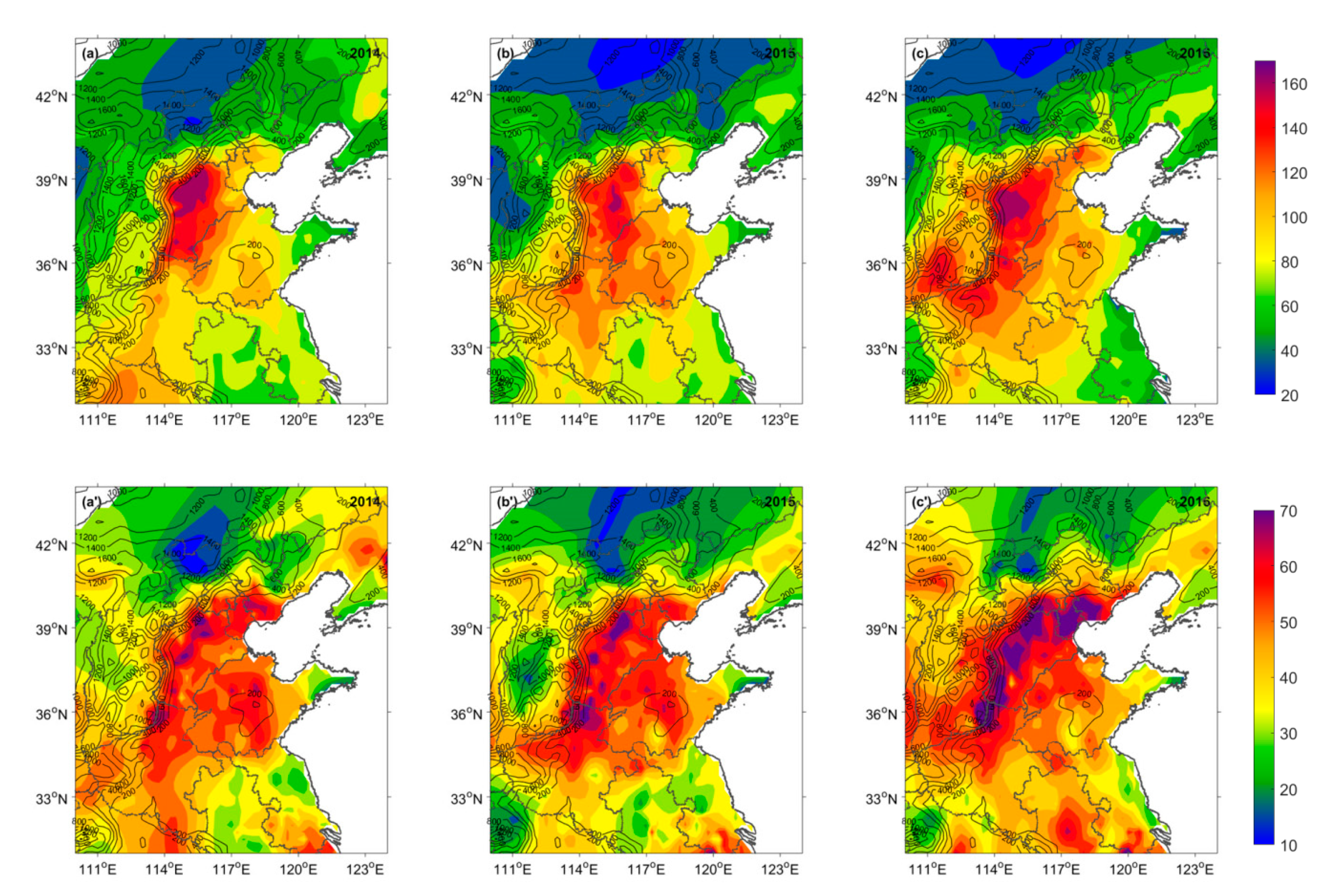
The data from about 1400 atmospheric component ground observation stations in Central and Eastern China (about 220 of them are in the BTH region) were linearly interpolated to 0.25° × 0.25° latitude and longitude grid space. In order to focus on the scope of this study, Figure 3 only shows the spatial distribution of PM_2.5 and NO₂ concentration ground observations in North China in 2014, 2015, and 2016. From the mean concentration of pollutants in the BTH region in winter, it can be found that the spatial distributions of PM_2.5 in 2014, 2015, and 2016 were generally similar (Figure 3a–c), and the pollution level was high in the North China Plain, which is surrounded by plateaus and mountains. The average concentration in the region exceeded 100 μg·m⁻³. The highest concentration was located in the south-central part of the BTH region and the northern part of Henan, with a maximum concentration of 200 μg·m⁻³ or greater, which resulted in a northeast–southwest high-pollution zone along the topography of the EMLP (or Taihang Mountain). However, the concentration of PM_2.5 in the LP west of Taihang Mountain decreased significantly. The distribution of NO₂ was similar to that of PM_2.5 along the topography (Figure 3a’–c’).

The distribution of wind fields and pollutants on four selected days (Figure 4) indicates that the daily distribution of pollutants has changed dramatically and both the intensity and impact scope of pollution changed significantly, indicating that the daily evolution of the weather system or the wind field determines the distribution and changes of the state of pollution under a certain background of emissions. Obviously, pollutants are driven by the wind, and the regions with the highest concentrations of pollution are at the front of the dominant wind. Such results indicate that different weather systems or wind fields have different effects on the distribution and accumulation of pollutants. 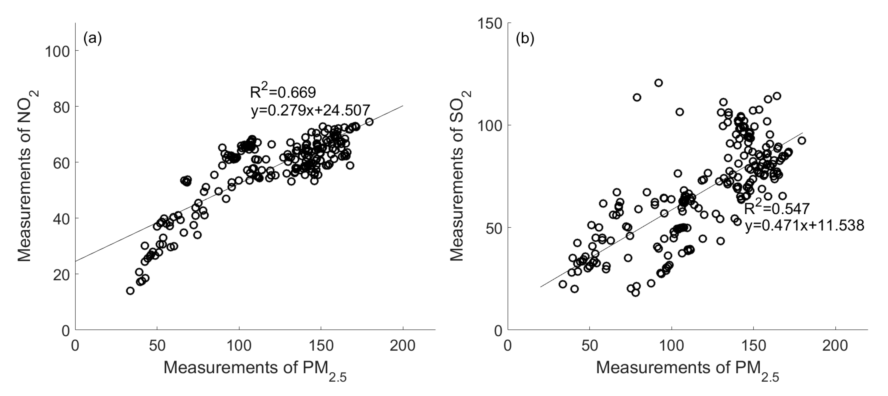The spatiotemporal distribution of pollutants (Figure 4) also shows that there is a synchronous change between NO₂ and PM_2.5. The correlation coefficients among PM_2.5, NO₂, and SO₂ in the BTH region in the winter of 2014, 2015, and 2016 were calculated (Figure 5a,b), with the spatial correlation coefficient between PM_2.5 and NO₂ reaching 0.82, and that between SO₂ and PM_2.5 reaching 0.74. The above correlation coefficients all passed the 99% significance test.

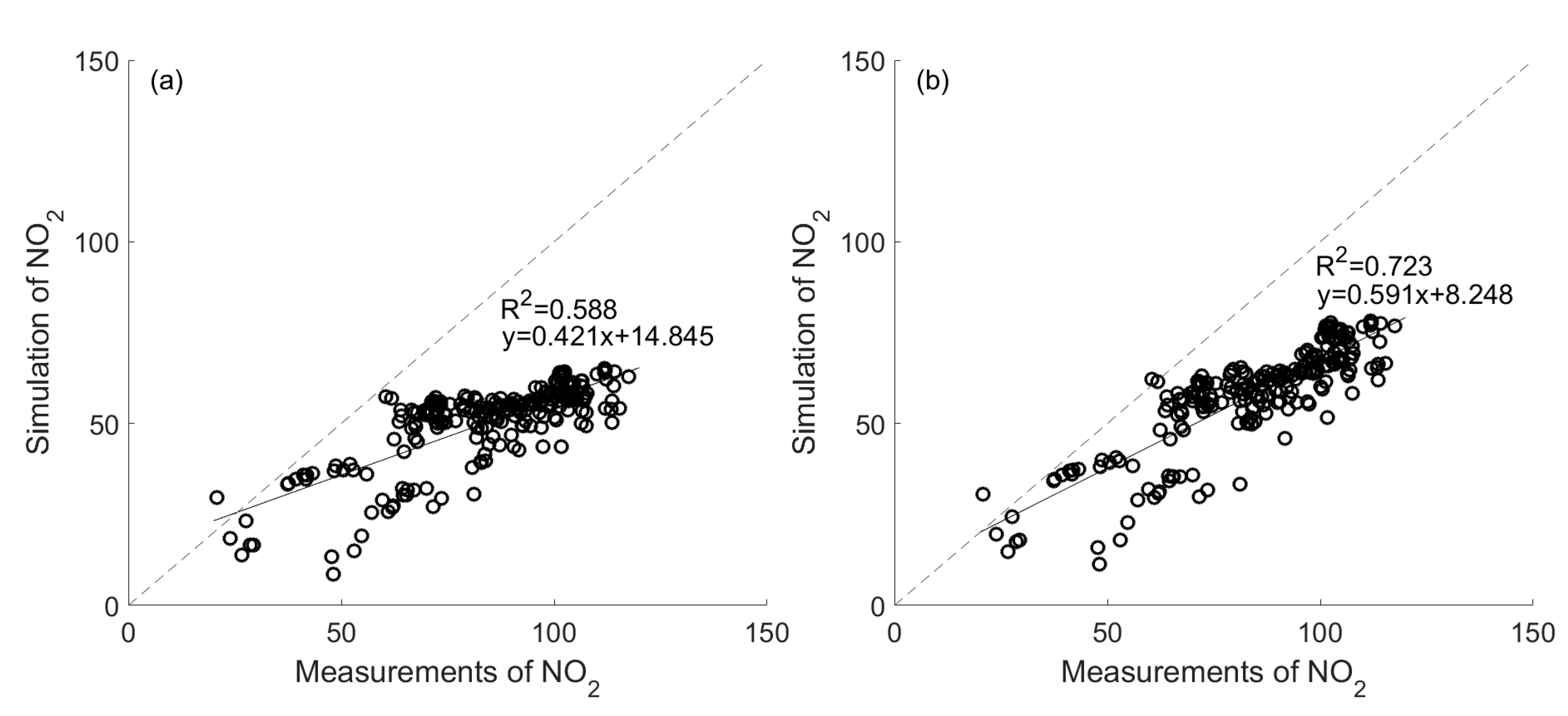
PM_2.5 is the primary pollutant in the BTH region during winter, and its correlation with NO₂ is higher than that with SO₂. The results presented in Section 2.2.3 show that the EMC of NO₂ had a higher reliability. In this study, we used NO₂ observations and EMC to analyze the causes of the spatial distribution of pollutants accumulated in the piedmont under the combined influence of the plateau topography and meteorological conditions.

3.2. Weak Wind Zone Background

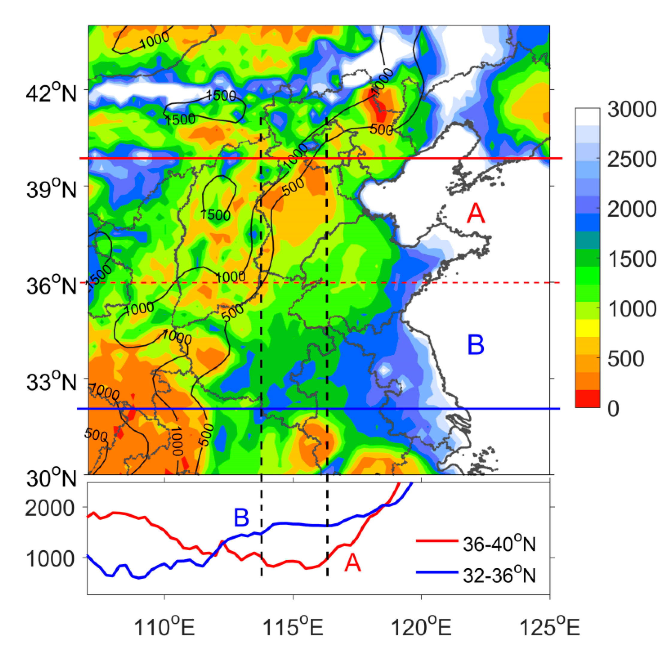
In winter, the leeward slope of the LP experiences a significant downdraft influenced by the topography of the plateau, resulting in weaker near-surface winds [13,14]. According to the distribution of average winter ventilation in 2016 (Figure 6), the distribution of ventilation across North China Plain was uneven. The highest ventilation was in the East China Sea, and the atmospheric diffusion conditions in the LP and the East China Plain were relatively good. In the topographic highs and lows of the central and southern parts of the BTH region, the atmospheric diffusion conditions were relatively poor. From the 36° to 40° N zonal average ventilation curve (the lower panel in Figure 6), it can be seen that the region from 114° to 117° E corresponded to the topographic transition from the plateau to the plain, which is a valley of atmospheric ventilation. Weak background wind field is not conducive to the diffusion of pollutants, and there is a substantial accumulation of pollutants in the weak wind zone on the EMLP. As a comparison, the atmospheric diffusion conditions in Henan and Shandong in the southern region (32°–36° N) were better.

3.3. Convergence Zone of Pollution on the EMLP

The results presented in Section 2.2.3 show that the EMC of NO₂ had high reliability. The results presented in Section 3.1 show that the correlation coefficient between PM_2.5 and NO₂ is very high in recent years. We used NO₂ observations and model-constraint EMC to analyze the causes of the spatial distribution of pollutants accumulated in the piedmont under the combined influence of the plateau topography and meteorological conditions. 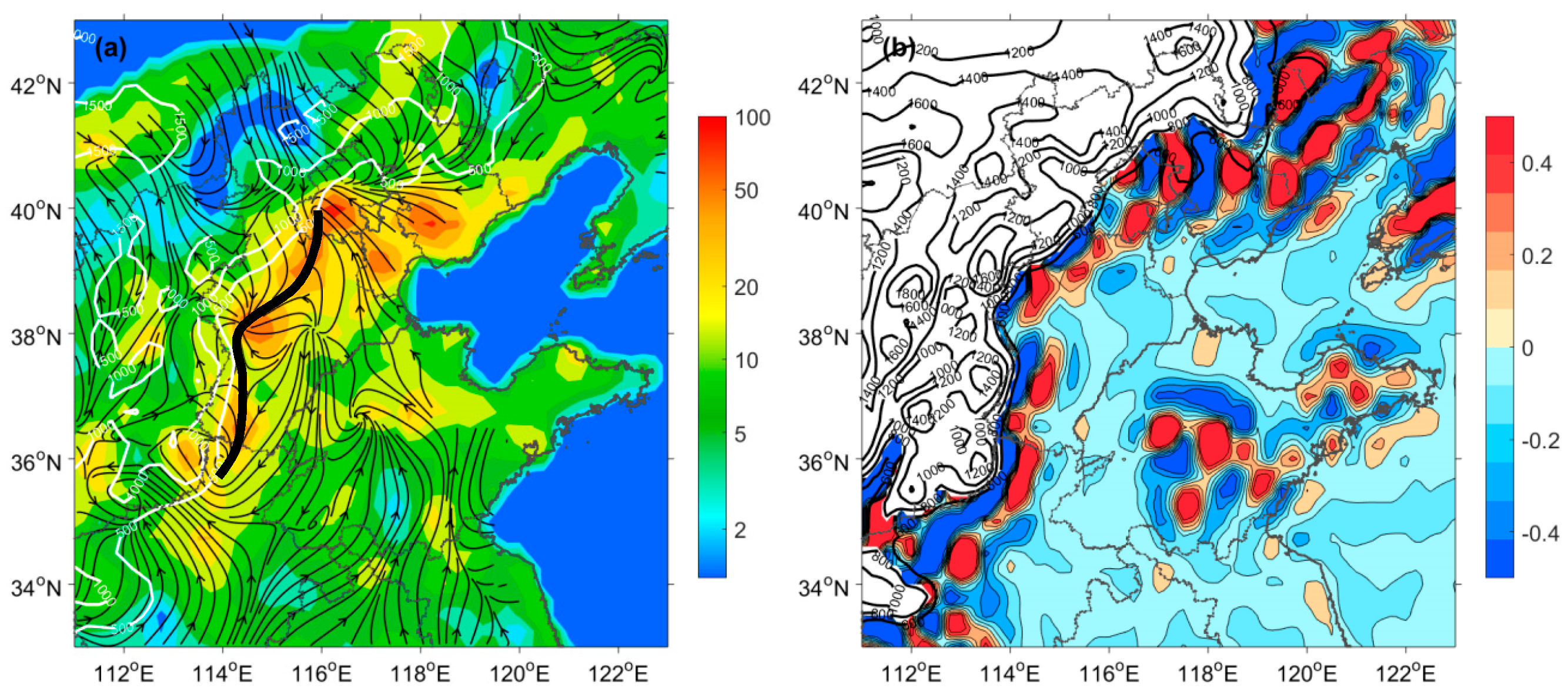Figure 7a shows the correlation coefficient vector calculated by using the EMC of NO₂ and the 975 hPa wind field data from 1 December 2016 to 31 January 2017. Correlation coefficient vector is the point-to-point correlation coefficient between EMC and 975 hPa wind field, which gives the correlation coefficient vector field in the x and y directions. The figure shows that there is a northeast–southwest convergent line along Beijing, to Central and Southern Hebei and the north of Henan, which indicates that the pollutants emitted into the atmosphere converge in this zone. By comparing the topographic distribution of such zones, it is found that the convergence line is near the EMLP (or Taihang Mountain), indicating that the convergence line is probably related to the interaction between the leeward airflows and the wind field in the eastern plain. Under the combined effects of plateau topography and circulation, a pollution zone tends to form on the EMLP.

We calculated the vertical vorticity using NCEP 975 hPa wind data from 1 December 2016 to 31 January 2017 and processed the vorticity field by using the filtering method, and then subtracted the filtered vorticity from the calculated original vorticity. The sub-synoptic scale vorticity field is then obtained, as shown in Figure 7b. It can be seen that there is a significant north–south chained vortex sequence on the EMLP (Figure 7b), which is generated by the vortex effect of the airflow over the leeward slope of the Loess Plateau [24]. The vorticity chains correspond to the correlation vector convergence and the accumulation of pollutant in Figure 7a. Combined with the WINEMIS of NO₂ (Figure 7a), the convergence line overlaps the high emission zone in the BTH region. For high emissions, the combination of topography and horizontal wind fields promote the formation of typical pollution transport pathways in the North China Plain in the EMLP, during the winter.

The correlation coefficient vector from Tianjin to Beijing exhibits a consistent south-easterly wind, indicating that Beijing is affected by the emissions from upstream of Tianjin, and such wind transports pollutants downstream. When the pollutant stream encounters the mountainous regions to the northwest, the pollutants will accumulate there.

3.4. The Influence of Plateau on the Vertical Diffusion of Pollutants

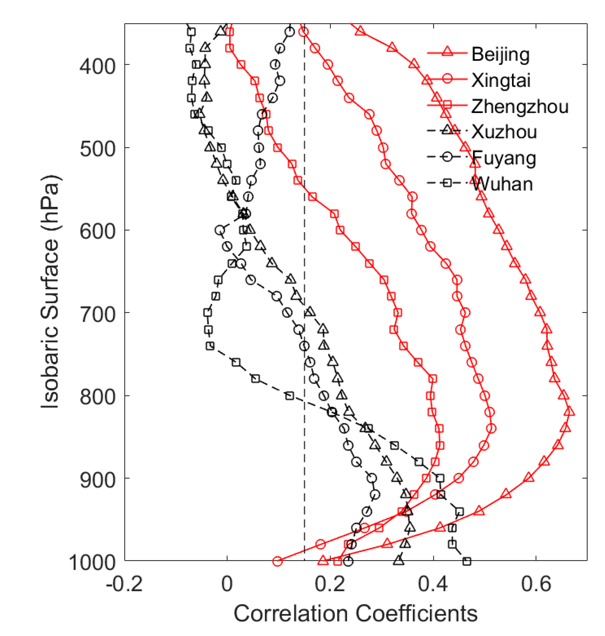
In this section, we cover representative stations both near to (Beijing, Xingtai, and Zhengzhou) and far from (Xuzhou, Fuyang, and Wuhan) the plateau (Figure 1), to investigate the effects of the plateau on the vertical diffusion of pollutants. Zhu et al. [13] calculated the vertical correlation coefficient profiles between the PM_2.5 concentration and air temperature by using the L-band sounding data and the daily averaged PM_2.5 concentration data from January 2016 to January 2017 in Beijing. In this study, we analyzed the differences in atmospheric thermal structures at different distances from the plateau and the vertical diffusion of pollutants by calculating the correlation coefficient profiles between the observed concentration of NO₂ and the L-band sounding temperature for the winters of 2014, 2015, and 2016 (Figure 8). The correlation coefficients of all sites below 800 hPa passed the 99% confidence test. The correlation coefficient profiles show that the three stations near the plateau exhibit a strong inversion profile, which is similar to the inversion layer of temperature sounding. The near-surface temperature is low, and the upper temperature increases rapidly, forming a stable atmospheric stratification, which inhibits the vertical diffusion of pollutants and causes pollutants to accumulate in a narrow space near the ground. The correlation coefficient profiles of the Xuzhou and Fuyang stations, which are both located far away from the plateau, have similar inverse thermal structures, but the horizontal span of the inversion temperature is very small, i.e., the inversion intensity is weak. Meanwhile, the correlation coefficient profile of the Wuhan station does not exhibit an obvious inversion structure. Additionally, the inversion layers of the stations near the plateau are deep and extend upward to 850 hPa, whereas the inversion layers of the stations far away from the plateau are below 900 hPa. Such difference in thermal structures at different distances from the plateau might be related to the regional circulation under the influence of the plateau and large-scale topography. The above analysis shows that a “warm cover” is often formed in the air above the plateau, and under its influence, there is a strong inhibitory effect that hinders the vertical diffusion of pollutants.

3.5. Differences in the Influence of Emissions under Different Weather Conditions

In this section, we will discuss the typical weather conditions affecting air quality in the BTH region during the period from 1 December 2016 to 31 January 2017. South-westerly winds, north-easterly winds, south-easterly winds, stagnant air, and north-westerly winds are the five typical wind conditions in the BTH region, and they were used to analyze the effects of different weather conditions or wind fields on pollution conditions. The selected weather processes maintain consistent wind field characteristics within the BTH region. In the two-month period, the number of days of south-westerly winds, stagnant air, north-easterly winds, south-easterly winds, and north-westerly winds were 14, 11, 8, 6, and 8, respectively. We first compare the EMC of each day with the two-month average of EMC (WINEMIS), i.e., (EMC-WINEMIS)/WINEMIS. We then classify the daily (EMC-WINEMIS)/WINEMIS results based on the corresponding wind field conditions. Therefore, the spatial distribution of the vulnerability of air pollution under different wind field conditions can be quantitatively analyzed.

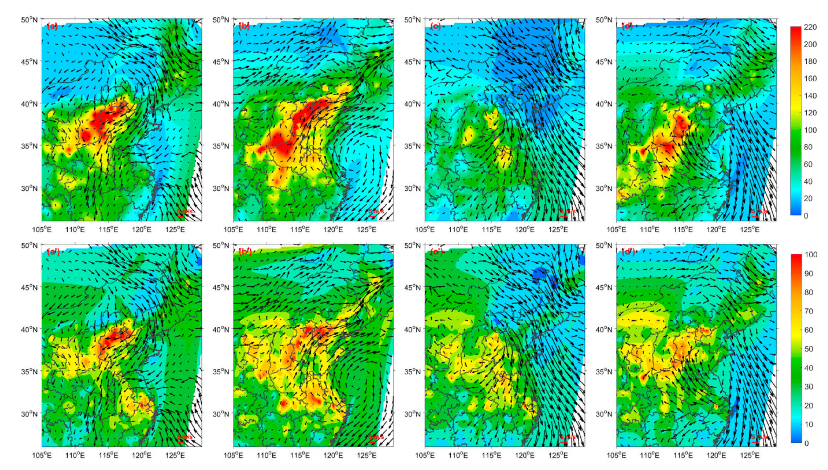
Figure 9a–e shows the relative deviations between the average EMC under different weather conditions and the WIN-EMIS. From this deviation, we can recognize and quantify the significant spatial differences in the effects of emission sources under different meteorological conditions in the BTH region. As shown in Figure 9a, under the influence of a south-westerly wind, the significant pollutants’ accumulation area is located near the eastern foothills of the Taihang Mountains and the southern slopes of the Yan Mountains. The south-westerly wind amplifies the effects of emissions by an average of 50% to 150% in the region, which results in the intensification of pollution and deterioration of the air quality in the regions along the mountains. Under the north-easterly prevailing winds (Figure 9b), the emission effect is increased significantly at the southern slope of Yanshan Mountain and the northeast side of Taihang Mountain. Under the south-easterly prevailing winds (Figure 9c), the effects of emissions on the Southeastern BTH region increase. Under the stagnant air (Figure 9d), the scope of high-impact pollution increases, and most of the effects of emissions on the BTH region increase. These four typical weather patterns cause various air pollution patterns and different emission effects. However, the most influential regions are primarily concentrated within 200 km of the east side of the plateau. Among these weather patterns, the south-westerly prevailing wind and the stagnant air conditions are most common in the BTH region during the winter. Such weather patterns have a significant multiplier effect on pollution emissions in the region, thereby maximizing regional pollution emissions.

The distribution characteristic of PM_2.5 showed differences under the influence of the four different types of prevailing wind systems. Figure 9a’ shows that, under the influence of south-westerly winds, the high PM_2.5 concentration area was concentrated in the Piedmont region, which was consistent with the emission pattern presented in Figure 9a, which highlighted the impact of the emission effect. The average concentration of PM_2.5 in front of the mountain was 200 μg·m⁻³ or greater. Under the influence of north-easterly prevailing winds (Figure 9b’), the high PM_2.5 concentration was concentrated in the region east of the Taihang Mountains. Under the south-easterly prevailing winds (Figure 9c’), the highest concentration of PM_2.5 was still concentrated in the piedmont of the Taihang Mountain due to the northwest direction of atmospheric transport. Under the stagnant air conditions (Figure 9d’), the concentrations of PM_2.5 in the plain regions were generally high, with an average of over 200 μg·m⁻³. From the analyses of the above emission effects and the distributions of PM_2.5, we concluded that large amounts of pollutants are often concentrated along the EMLP in the BTH region during winter. Therefore, the EMLP has become the most heavily polluted region, which is consistent with the distribution of winter pollutants presented in Section 3.1.

Because of strong winds and low emissions upstream, the north-westerly wind typically has a pollution-removal effect in the BTH region, and the intensity of the EMC is significantly lower than that of the WINEMIS (Figure 9e,e’). The north-westerly wind has the most significant impact on Beijing, Tianjin, and the eastern border of the Taihang Mountains, where PM_2.5 concentrations have declined significantly.

3.6. Comprehensive Causes of “Vulnerable Regions” of Pollution in the BTH Region

The terrain of the BTH region is complex. The northern Yan Mountains and the western LP (or Mt. Taihang) form a boundary that partially encloses the region, and there is a large area of open terrain to the south. A weak wind zone is created on the EMLP due to the influence of the plateau and mountains on the regional atmospheric circulation. Additionally, a north–south sub-synoptic scale vortex circulation sequence is formed on the EMLP, and the corresponding wind field convergence between the positive and negative vorticity sequences form a significant convergence zone of pollutants (Figure 7). The “warm-cover” formed by a temperature anomaly over the EMLP inhibits the vertical diffusion of pollutants. These mechanisms force pollutants to converge in a strip on the EMLP. When south-westerly and north-easterly winds prevail, the pollution belts move longitudinally to the north and south along the boundary of the EMLP under the impetus of the wind fields. In this situation, pollution persists in the EMLP. The north–south “vortex sequence” formed along the EMLP terrain is similar to the “train effect” of pollution (Figure 7b). Therefore, south-westerly and north-easterly winds are more conducive to maintaining a prolonged haze event in addition to the regional transport of pollutants. The south-westerly wind causes pollutants to accumulate to the south of the Yan Mountains, which intensifies the haze in Beijing and Tianjin. Under the influence of the above-mentioned atmospheric dynamical and thermal processes, the EMLP has become a “vulnerable region” to haze pollution because its meteorological condition is unfavorable to the spread and diffusion of pollutants, which means that the region is more vulnerable to air pollution even in the same emission background. The above mechanisms also explain the centralization of pollutants along the plateau noted in Section 3.1. In recent years, although the governments of Beijing, Tianjin, and Hebei have increased the efforts to control air pollution, the intensity of pollution emissions is still high. This fact, combined with the vulnerability to air pollution and the frequent adverse weather conditions, has made the region the most polluted area in China.

4. The Cross-Year Haze Event of 2016–2017

There was a long period of heavy haze in the BTH region from 29 December 2016 to 7 January 2017. During this pollution period, high concentrations of pollutants were primarily concentrated in the BTH, Shandong, northern Henan, and Guanzhong. The air quality in these regions reached heavy (MEPC, HJ6333-2012) or severe pollution levels. The haze pollution was obviously heavier in the BTH region than that in other regions. On 1 January and 4 January 2017, the PM_2.5 concentrations in Beijing reached two peaks, both exceeding 500 μg·m⁻³.

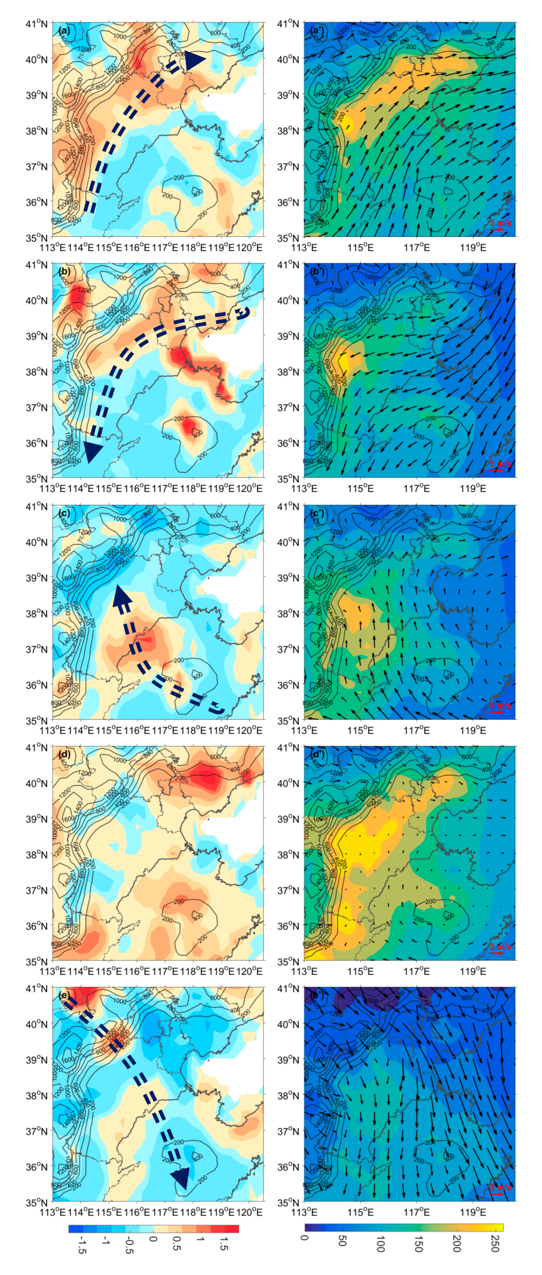
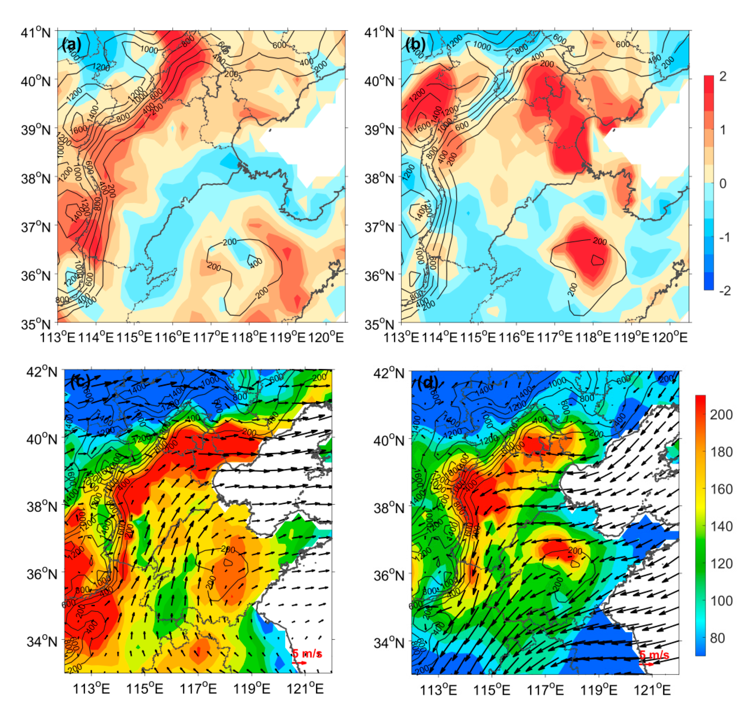
In the first six days of the haze event (29 December 2016 to 3 January 2017), the high-pressure system was located on the eastern coast of China, and the south-westerly wind dominated the lower atmosphere of the BTH region (Figure 10a,c). According to the analyses in Section 3.5, the emission effect at the EMLP was enhanced, and the pollutants converged into strips and moved longitudinally under the influence of the south-westerly wind. The “train effect” caused pollutants to be blocked, which made them accumulate at the Yan Mountains and the cities along the Taihang Mountains. Beijing, Tianjin, and Tangshan experienced persistent haze. At the later stage of the haze event (4 January to 7 January 2017) (Figure 10b,d), cold air moved from northeast to southwest, and the pollutants converged on the EMLP, where the haze persisted. By analyzing this process, we find that pollutants were concentrated in the regions along the mountains under the influence of the plateau and large terrain, which is caused by the unique thermal and dynamic processes. With the alternating dominance of south-westerly and north-easterly winds, the pollutants oscillate in the north–south direction along the mountainous region, which leads to the long-term persistence of haze pollution.

5. Conclusions

Surrounded by the “semi-enclosed” and the southward-opening terrain formed by the LP, a contamination conveyor belt is distributed along the topography of the EMLP in the BTH region. In this study, based on the innovative adaptive nudging constraint method, we quantitatively analyzed the differences in the influence of emission sources under different dynamic and thermal conditions in the BTH region, which is impacted by a special large-scale leeward slope terrain. The mechanism of air pollution vulnerability in the BTH region and the comprehensive effects of terrain–meteorological conditions on air pollution were also discussed.

The weak atmospheric ventilation on the EMLP is not conducive to the diffusion and dilution of pollutants. Additionally, under the influence of topography, a north–south vortex circulation sequence of the sub-synoptic scale is formed. The convergence of the wind fields corresponding to the positive and negative vorticity sequences results in a significant convergence of pollution. The convergence line passed from Beijing to Central and Southern Hebei and to the north part of Henan. The pollutants released into the atmosphere tend to converge in this strip zone. The “warm cover” formed over the upper air of the EMLP hinders the vertical diffusion of pollutants. Due to the influence of plateau topography and regional atmospheric circulation, the EMLP has become a “naturally vulnerable region” to haze pollution, which is unfavorable to pollutant diffusion.

There are significant spatial differences in the effects of emission sources under different meteorological conditions or wind field patterns. We quantitatively analyzed the effects and distribution characteristics of emission sources under different meteorological conditions in the BTH region for a two-month period. Under the predominant south-westerly winds, pollutants tended to accumulate near the eastern foothills of the Taihang Mountains and the south of the Yan Mountains. Under the influence of north-easterly winds, pollutants were concentrated in the south of Yan Mountain and the northeastern side of the Taihang Mountains. Under the predominant south-easterly winds, the southeastern part of the BTH region was the most vulnerable region to pollution. In the case of stagnant air, the impact of emissions in most areas of BTH is significantly enhanced. Such wind fields amplified the effects of emissions by an average of 50% to 150% in the EMLP. When southwest and northeast winds alternated, the pollution belt moved longitudinally along the south–north direction of the EMLP under the impetus of the wind fields. The north–south “vortex sequence” along the EMLP mimicked the “train effect” of pollution, which caused continuous pollution conditions in the EMLP. Although different weather systems have different effects on the distribution and accumulation of pollutants, the regions with the greatest impact on emissions were all located in the Piedmont region, indicating that such regions are more vulnerable to severe air pollution.

References

1. An, X.; Zhu, T.; Wang, Z.; Li, C.; Wang, Y. A modeling analysis of a heavy air pollution episode occurred in Beijing. Atmos. Chem. Phys. 2007, 7, 3103–3114. [Google Scholar] [CrossRef]
2. Fu, G.Q.; Xu, W.Y.; Rong, R.F.; Li, J.B.; Zhao, C.S. The distribution and trends of fog and haze in the North China Plain over the past 30 years. Atmos. Chem. Phys. 2014, 14, 16123–16149. [Google Scholar] [CrossRef]
3. Gang, L.; Fu, J.; Dong, J.; Hu, W.; Dong, D.; Huang, Y.; Zhao, M. Spatio-temporal variation of PM2.5 concentrations and their relationship with geographic and socioeconomic factors in China. Int. J. Environ. Res. Public Health 2014, 11, 173–186. [Google Scholar]
4. Cao, J.J. PM2.5 and the Environment in China; Science Press: Beijing, China, 2014. [Google Scholar]
5. Huang, R.J.; Zhang, Y.; Bozzetti, C.; Ho, K.F.; Cao, J.J.; Han, Y.; Daellenbach, K.R.; Slowik, J.G.; Platt, S.M.; Canonaco, F. High secondary aerosol contribution to particulate pollution during haze events in China. Nature 2014, 514, 218. [Google Scholar] [CrossRef] [PubMed]
6. Schlesinger, R.B. The health impact of common inorganic components of fine particulate matter (PM2.5) in ambient air: A critical review. Inhal. Toxicol. 2007, 19, 811. [Google Scholar] [CrossRef] [PubMed]
7. Zhang, X.Y.; Wang, J.Z.; Wang, Y.Q.; Liu, H.L.; Sun, J.Y.; Zhang, Y.M. Changes in chemical components of aerosol particles in different haze regions in China from 2006 to 2013 and contribution of meteorological factors. Atmos. Chem. Phys. 2015, 15, 12935–12952. [Google Scholar] [CrossRef]
8. Hong, H. Formation Mechanism and Control Strategies of Haze in China; Bulletin of Chinese Academy of Sciences: Beijing, China, 2013. [Google Scholar]
9. Liu, F.; Beirle, S.; Zhang, Q.; Rj, V.D.A.; Zheng, B.; Tong, D.; He, K. NOx emission trends over Chinese cities estimated from OMI observations during 2005 to 2015. Atmos. Chem. Phys. 2017, 17, 9261. [Google Scholar] [CrossRef]
10. Krotkov, N.A.; Mclinden, C.A.; Li, C.; Lamsal, L.N.; Celarier, E.A.; Marchenko, S.V.; Swartz, W.H.; Bucsela, E.J.; Joiner, J.; Duncan, B.N. Aura OMI observations of regional SO2 and NO2 pollution changes from 2005 to 2015. Atmos. Chem. Phys. 2016, 16, 4605–4629. [Google Scholar] [CrossRef]
11. Li, H.; Zhang, Q.; Zhang, Q.; Chen, C.; Wang, L.; Wei, Z.; Zhou, S.; Parworth, C.; Zheng, B.; Canonaco, F. Wintertime aerosol chemistry and haze evolution in an extremely polluted city of the North China Plain: Significant contribution from coal and biomass combustion. Atmos. Chem. Phys. 2017, 17, 4751–4768. [Google Scholar] [CrossRef]
12. Yin, Z.; Wang, H.; Chen, H. Understanding severe winter haze pollution in the north-central North China Plain in 2014. Atmos. Chem. Phys. 2016. [Google Scholar] [CrossRef]
13. Zhu, W.; Xu, X.; Zheng, J.; Yan, P.; Wang, Y.; Cai, W. The characteristics of abnormal wintertime pollution events in the Jing-Jin-Ji region and its relationships with meteorological factors. Sci. Total Environ. 2018, 626, 887–898. [Google Scholar] [CrossRef] [PubMed]
14. Xu, X.; Zhao, T.; Liu, F.; Gong, S.L.; Kristovich, D.; Lu, C.; Guo, Y.; Cheng, X.; Wang, Y.; Ding, G. Climate modulation of the Tibetan Plateau on haze in China. Atmos. Chem. Phys. 2016, 15, 28915–28937. [Google Scholar] [CrossRef]
15. Bei, N.; Li, G.; Huang, R.J.; Cao, J.; Meng, N.; Feng, T.; Liu, S.; Zhang, T.; Zhang, Q.; Molina, L.T. Typical synoptic situations and their impacts on the wintertime air pollution in the Guanzhong basin, China. Atmos. Chem. Phys. 2016, 16, e7387. [Google Scholar] [CrossRef]
16. Wu, P.; Ding, Y.; Liu, Y. Atmospheric circulation and dynamic mechanism for persistent haze events in the Beijing–Tianjin–Hebei region. Adv. Atmos. Sci. 2017, 34, 429–440. [Google Scholar] [CrossRef]
17. Xu, W.Y.; Zhao, C.S.; Ran, L.; Deng, Z.Z. Characteristics of pollutants and their correlation to meteorological conditions at a suburban site in the North China Plain. Atmos. Chem. Phys. 2011, 11, 4353–4369. [Google Scholar] [CrossRef]
18. Zhang, J.P.; Zhu, T.; Zhang, Q.H.; Li, C.C.; Shu, H.L.; Ying, Y.; Dai, Z.P.; Wang, X.; Liu, X.Y.; Liang, A.M. The impact of circulation patterns on regional transport pathways and air quality over Beijing and its surroundings. Atmos. Chem. Phys. 2012, 11, 33465–33509. [Google Scholar] [CrossRef]
19. Zhao, X.J.; Zhao, P.S.; Xu, J.; Meng, W. Analysis of a winter regional haze event and its formation mechanism in the North China Plain. Atmos. Chem. Phys. 2013, 13, 5685–5696. [Google Scholar] [CrossRef]
20. Wu, F.; Xie, P.; Li, A.; Mou, F.; Chen, H.; Zhu, Y.; Zhu, T.; Liu, J.; Liu, W. Investigations of Temporal and Spatial Distribution of Precursors SO2 and NO2 Vertical Columns in North China Plain by Mobile DOAS. Atmos. Chem. Phys. 2018, 18, 1535–1554. [Google Scholar] [CrossRef]
21. Zhang, R.H.; Qiang, L.; Zhang, R.N. Meteorological conditions for the persistent severe fog and haze event over eastern China in January 2013. Sci. China Earth Sci. 2014, 57, 26–35. [Google Scholar]
22. Bei, N.; Zhao, L.; Wu, J.; Li, X.; Feng, T.; Li, G. Impacts of sea-land and mountain-valley circulations on the air pollution in Beijing-Tianjin-Hebei (BTH): A case study. Environ. Pollut. 2017, 234, 429. [Google Scholar] [CrossRef]
23. Miao, Y.; Liu, S.; Zheng, Y.; Wang, S.; Chen, B. Numerical study of the effects of topography and urbanization on the local atmospheric circulations over the Beijing-Tianjin-Hebei, China. Am. Econ. Rev. 2003, 93, 431–435. [Google Scholar] [CrossRef]
24. Xu, X.; Wang, Y.J.; Zhao, T.L.; Cheng, X.H.; Meng, Y.Y.; Ding, G.A. “Harbor” effect of large topography on haze distribution in eastern China and its climate modulation on decadal variations in haze. Chin. Sci. Bull. 2015, 60, 1132. [Google Scholar]
25. Xu, X.; Guo, X.; Zhao, T.; An, X.; Zhao, Y.; Quan, J.; Mao, F.; Gao, Y.; Cheng, X.; Zhu, W. Are precipitation anomalies associated with aerosol variations over Eastern China? Atmos. Chem. Phys. 2017, 17, 8011. [Google Scholar] [CrossRef]
26. Nair, V.G.; Mohanakumar, K. A Modelling Study in Mountain Meteorology: Impact of Western Ghats Orography on the Weather and Climate of South India; VDM Verlag Dr. Müller: Saarbrücken, Germany, 2006. [Google Scholar]
27. Whiteman, C.D.; Mckee, T.B. Air pollution implications of inversion descent in mountain valleys. Atmos. Environ. 1978, 12, 2151–2158. [Google Scholar] [CrossRef]
28. Guniya, G.S.; Tskvitinidze, Z.I.; Kholmatzhanov, B.M.; Fatkhullaeva, Z.N. Foehn influence on air pollution processes in the mountain regions. Rus. Meteorol. Hydrol. 2010, 35, 406–410. [Google Scholar] [CrossRef]
29. Xu, X.; Zhou, L.; Zhou, X.; Yan, P.; Weng, Y.; Tao, S.; Mao, J.; Ding, G.; Bian, L.; Chan, J. Influential fields of peripheral sources of severe urban atmospheric polluting process. Sci. China 2004, 34, 958–966. [Google Scholar]
30. Xu, X.; Xie, L.; Cheng, X.; Xu, J.; Zhou, X.; Ding, G. Application of an adaptive nudging scheme in air quality forecasting in China. J. Appl. Meteorol. Climatol. 2008, 47, 2105–2114. [Google Scholar] [CrossRef]
31. Byun, D.W. Dynamically consistent formulations in meteorological and air quality models for multiscale atmospheric studies. Part I: Governing equations in a generalized coordinate system. J. Atmos. Sci. 1999, 56, 3789–3807. [Google Scholar] [CrossRef]
32. Dennis, R.L.; Byun, D.W.; Novak, J.H.; Galluppi, K.J.; Vouk, C.J.C.A. The next generation of integrated air quality modeling: EPA’s models-3. Atmos. Environ. 1996, 30, 1925–1938. [Google Scholar] [CrossRef]
33. Seinfeld, J.H.; Pandis, S.N. Atmospheric Chemistry and Physics: From Air Pollution to Climate Change; John Wiley & Sons, Inc.: Hoboken, NJ, USA, 2016. [Google Scholar]
34. Kain, J.S.; Fritsch, J.M. A one-dimensional entraining/detraining plume model and its application in convective parameterization. J. Atmos. Sci. 1990, 47, 2784–2802. [Google Scholar] [CrossRef]
35. Pleim, J.E. A combined local and nonlocal closure model for the atmospheric boundary layer. Part I: Model description and testing. J. Appl. Meteorol. Clim. 2007, 46, 1383–1395. [Google Scholar] [CrossRef]
36. Hong, S.Y.; Lim, J.O.J. The WRF single-moment 6-class microphysics scheme (WSM6). Asia Pac. J. Atmos. Sci. 2006, 42, 129–151. [Google Scholar]
37. Iacono, M.J.; Mlawer, E.J.; Clough, S.A.; Morcrette, J.J. Impact of an improved longwave radiation model, RRTM, on the energy budget and thermodynamic properties of the NCAR community climate model, CCM3. J. Geophys. Res. 2000, 105, 14873–14890. [Google Scholar] [CrossRef]
38. Ek, M.B.; Mitchell, K.E.; Lin, Y.; Rogers, E.; Grunmann, P.; Koren, V.; Gayno, G.; Tarpley, J.D. Implementation of Noah land surface model advances in the National Centers for Environmental Prediction operational mesoscale Eta model. J. Geophys. Res. 2003, 108, GCP 12-1. [Google Scholar] [CrossRef]
39. Yamartino, R.J. Improvements to horizontal transport in grid models. In Air Pollution Modeling & Its Application XIII; Springer: Boston, MA, USA, 2000; pp. 67–73. [Google Scholar]
40. Mascagni, M. The backward euler method for numerical solution of the hodgkin-huxley equations of nerve conduction. Siam J. Numer. Anal. 1990, 27, 941–962. [Google Scholar] [CrossRef]
41. The University of North Carolina. SMOKE v3.6 User’s Manual; The Institute for the Environment: Chapel Hill, NC, USA, 2014. [Google Scholar]
42. Meng, K.; Cheng, X.; Xu, X.; Qu, X.; Ma, C.; Zhao, Y.; Li, Y.; Yang, Y.; Zhang, W.; Ding, G. Spatial-temporal variations of pollutant emission sources inversed by adaptive nudging scheme over Beijing-Tianjin-Hebei region based on the CMAQ model. Acta Sci. Circum. 2017, 37, 52–60. [Google Scholar]
43. Cheng, X.H.; Xu, X.D.; Ding, G.A. An emission source inversion model based on satellite data and its application in air quality forecasts. Sci. China Earth Sci. 2010, 53, 752–762. [Google Scholar] [CrossRef]
44. Meng, K.; Xu, X.; Cheng, X.; Xu, X.; Qu, X.; Zhu, W.; Ma, C.; Yang, Y.; Zhao, Y. Spatio-temporal variations in SO2 and NO2 emissions caused by heating over the Beijing-Tianjin-Hebei region constrained by an adaptive nudging method with OMI data. Sci. Total Environ. 2018, 642, 543–552. [Google Scholar] [CrossRef]
45. Xu, D.; Zhu, R. A study on the distribution of ventilation and rainout capacity in mainland China. J. Environ. Sci. China 1989, 9, 367–374. [Google Scholar]
Figure 1. Topographic distribution (meters above sea level) map of Central and Eastern China (1 km × 1 km). The red symbols represent the sounding stations near the plateau, and the black symbols represent the sounding stations far from the plateau.
Atmosphere 10 00719 g001
Figure 2. Comparison of the observed and simulated NO2 concentrations (μg·m−3): (a) comparison between the simulated results from M2012 and the observations; (b) comparison between the inversion simulated results and the observations.
Atmosphere 10 00719 g002
Figure 3. Maps of the observed PM2.5 and NO2 concentrations in winter (December–February) in Northern China (μg·m−3). (a) PM2.5, 2014; (b) PM2.5, 2015; (c) PM2.5, 2016; (a’) NO2, 2014; (b’) NO2, 2015; and (c’) NO2, 2016.
Atmosphere 10 00719 g003
Figure 4. Spatial patterns of daily average mass concentration (μg·m−3) of PM2.5 and NO2 overlaid with the 975 hPa wind fields (m·s−1) in the central part of Eastern China: (a) PM2.5, 12 December 2016; (b) PM2.5, 30 December 2016; (c) PM2.5, 13 January 2017; (d) PM2.5, 23 January 2017; (a’) NO2, 12 December 2016; (b’) NO2, 30 December 2016; (c’) NO2, 13 January 2017; and (d’) NO2, 23 January 2017.
Atmosphere 10 00719 g004
Figure 5. Scatter plots of the surface observations in the Beijing-Tianjin-Hebei (BTH) region (μg·m−3) for (a) PM2.5 and NO2, and (b) PM2.5 and SO2 in the winter of 2014–2016.
Atmosphere 10 00719 g005
Figure 6. Spatial patterns of the average ventilation (m2·s−1) in the North China Plain during the winter of 2016 (the upper panel); Longitudinal mean ventilation curve in 36–40° N (in red) and 32–36° N (in blue; the lower panel).
Atmosphere 10 00719 g006
Figure 7. (a) Correlation coefficient vector between the emissions with the consideration of meteorological conditions (EMC) and the 975 hPa wind fields. The color bar is the the intensity of emissions in winter (WINEMIS) values (in g·s−1). The thick solid black line is the correlation vector convergence line, and the solid white line is the elevation (in meters). (b) Distribution of sub-synoptic vorticity perturbations (10−5 s−1) at 975 hPa over the eastern margin of the Loess Plateau (EMLP). The solid black line is the elevation (in meters).
Atmosphere 10 00719 g007
Figure 8. The profiles of the correlation coefficient between the NO2 observations and the L-band air temperature observations. The red lines represent the sites near the plateau and the black lines represent the sites far away from the plateau. The grey vertical dotted line indicates a 99% reliability test.
Atmosphere 10 00719 g008
Figure 9. Spatial patterns of relative deviations between the average EMC under each weather condition and the WINEMIS (i.e., (EMC-WINEMIS)/WINEMIS) under (a) south-westerly; (b) north-easterly; (c) south-easterly; (d) stagnant air; (e) north-westerly. Distribution of corresponding PM2.5 concentrations (in colored shades; μg·m−3) overlaid with the 975 hPa mean wind fields (arrow; m·s−1) under (a’) south-westerly; (b’) north-easterly; (c’) south-easterly; (d’) stagnant air; (e’) north-westerly. The dark blue thick arrows indicate the prevailing wind direction.
Atmosphere 10 00719 g009
Figure 10. (a,b) Spatial patterns of relative deviations of the EMC and the WINEMIS from 29 December 2016 to 7 January 2017. (c,d) Distribution of PM2.5 mass concentrations (μg·m−3) overlaid with the 975 hPa average wind field (m·s−1). The panels (a,c) are for the distributions from 29 December 2016 to 3 January 2017, and the panels (b,d) are for the distributions from 4 January to 7 January 2017.
Atmosphere 10 00719 g010