Multi-Model Evaluation of Meteorological Drivers, Air Pollutants and Quantification of Emission Sources over the Upper Brahmaputra Basin

Abstract

The temporal distributions of meteorological drivers and air pollutants over Dibrugarh, a location in the upper Brahmaputra basin, are studied using observations, models and reanalysis data. The study aims to assess the performance of the Weather Research and Forecasting model coupled with chemistry (WRF-Chem), the WRF coupled with Sulfur Transport dEposition Model (WRF-STEM), and Copernicus Atmosphere Monitoring Service (CAMS) model over Dibrugarh for the first time. The meteorological variables and air pollutants viz., black carbon(BC), carbon monoxide(CO), sulphur dioxide(SO₂), Ozone(O₃), and oxides of Nitrogen(NO_x) obtained from WRF-Chem, WRF-STEM and CAMS are evaluated with observations. The source region tagged CO simulated by WRF-STEM delineate the regional contribution of CO. The principal source region of anthropogenic CO over Dibrugarh is North-Eastern India with a 59% contribution followed by that from China (17%), Indo-Gangetic Plains (14%), Bangladesh (6%), other parts of India (3%) and other regions (1%). Further, the BC-CO regression analysis is used to delineate the local emission sources. The BC-CO correlations estimated from models (0.99 for WRF-Chem, 0.96 for WRF-STEM, 0.89 for CAMS), and reanalysis (0.8 for Modern-Era Retrospective Analysis for Research and Applications, Version 2 (MERRA2) are maximum in pre-monsoon whereas surface observations show highest correlations (0.81) in winter. In pre-monsoon season, 90% of the modeled CO is due to biomass burning over Dibrugarh.

1. Introduction

Rising population, rapid urbanization, transportation, and economic growth are reportedly the major causes behind the serious issues of air pollution in South Asian countries like Bangladesh, India, Nepal, Pakistan and Sri Lanka [1,2,3,4]. Over the last decade, emissions from the power plant sector, petroleum refineries, oil sector, industrial and domestic sectors have increased considerably [5,6,7,8] over south-Asia. The maximum emissions of SO₂ in South Asia are from the industrial and power sectors, which contribute approximately 87%. However, the sources of emission vary from country to country. For example in Bangladesh, the main sources of SO₂ are vehicles, brick kilns, and the pulp and paper industry, etc. whereas in India the main sources are power plants, industries, etc. [9]. Among South Asian countries, India has been reported to be the second highest contributor of CO (12,000 GgY⁻¹), BC (83 GgY⁻¹) and SO₂ (74 GgY⁻¹) from the biomass burning sectors [10] and the highest contributor of CO from the domestic, industrial and road transport sectors [9]. According to Gurjar et al. [9], in India, major emission sources of BC are biofuel burning, biomass burning, and fossil fuel burning. Among Asian countries, India contributed 29% of the total emissions of BC [11]. NO_x is emitted mainly from vehicular emissions, industries, transport, agricultural residue burning and biomass burning [12].

A number of earlier studies in India have shown the impact of elevated CO, BC and SO₂ on local as well as regional air quality [5,13,14]. Apart from anthropogenic emissions, long-range transportation also plays a significant role in raising the pollutant levels over a region [15,16,17,18,19,20,21,22]. The emission rates of atmospheric trace gases like NO₂ and SO₂ occupy the highest levels after particulate matter in India, due to fast growing industries, economy, etc. [23]. Pollutants like CO and BC provide useful insights into understanding background air quality and also impact human health. BC, one of the primary pollutants is considered hazardous to the lungs and general health [24]. Rising air pollution in the Indian subcontinent is continuously degrading the ambient air quality [25,26,27,28,29] which is responsible for constantly rising numbers of death cases and respiratory illness [6,30].

Climate change is usually discussed in global terms; nevertheless, its effects vary quite significantly among different regions of the Earth [31]. Climate change has extensive effects on the sectors like water resources, agriculture, food security and human health [32]. The impact of climate change is more likely to have a bad effect on developing countries due to high dependency on climate-sensitive livelihoods like agriculture, water, and forestry [33]. The economy of North-Eastern India depends on agriculture, tea cultivation, etc., so the effect of air pollution may cause environmental degradation such as lowering of agricultural crop yields. The region is of great importance in terms of resources such as coal, oil/gas fields, oil refineries, tea industries, and brick kilns [34]. The pollutants emitted from these sectors have considerable impacts on the air quality of the region [15,34]. Industries usually rely on electricity for operations and maintenance; insufficient power availability often calls for the use of diesel generators (using coal, diesel, and heavy fuel oil), which release pollutants like SO₂, BC and others into the atmosphere, causing air pollution [35,36]. Oil wells during fires/blowouts release a large number of gases like CO, SO₂, hydrogen sulphide (H₂S), and hydrocarbons into the atmosphere [34]. The city of Dibrugarh located in the upper Brahmaputra basin of North-Eastern India is very rich in minerals and has large deposits of crude oil and coal [37,38]. The oil, brick kilns and natural gas fields located within 50–100 km from Dibrugarh are the local emission sources [15,19]. During winter and pre-monsoon seasons the concentrations of O₃, NO_x, SO₂, CO, PM_2.5, PM₁₀, and BC are higher at Dibrugarh [15,19,34]. This is attributed to biomass burning, local scale meteorology, planetary boundary layer height PBLH, transportation, etc. [38]. In previous studies, the National Oceanic and Atmospheric Administration (NOAA) HYSPLIT model has been used to identify the transport pathways of pollutants and their source regions over Dibrugarh. Bhuyan et al. [15] and Pathak et al. [38] in their studies have used the HYSPLIT back-trajectory and concentration weighted trajectory (CWT) analysis of trace gases such as NO_x, O₃ and CO to delineate the possible airmass trajectory and identify the potential source region of gases and their contribution over Dibrugarh.

However, the use of HYSPLIT have some limitations, as the meteorological data used in HYSPLIT model are available at relatively coarse temporal resolution (1–6 h), which can result in errors under rapidly changing conditions like dispersion, involving sea-breezes and mountain-valley circulations [39]. Gogoi et al. [34] highlighted the effects of aerosols over North-Eastern India using WRF-Chem and GOCART models. However, quantification of emission sources and regional contributions for this region has not been attempted so far.

The present study aims at assessing the temporal variations of near-surface meteorological drivers and air pollutants over Dibrugarh at daily timescales using multi-model (i.e., WRF-Chem, WRF-STEM, CAMS and HYSPLIT) and MERRA2 reanalysis datasets. It is worth mentioning that meteorology plays a significant role in the lifting/sinking of pollutants over a region via formation, transport, and dispersion of air pollutants [15,40]. In addition, statistical quantities are computed and intercompared with surface-based measurement data to enlighten the performance of the models, reanalysis data for the weather and climate study over the region in the future. This study uses STEM CO tracers to identify as well as quantify the emission sources and regional contributions over Dibrugarh. This study will further help in understanding air quality over a region where surface measurement data are not available and difficult to setup.

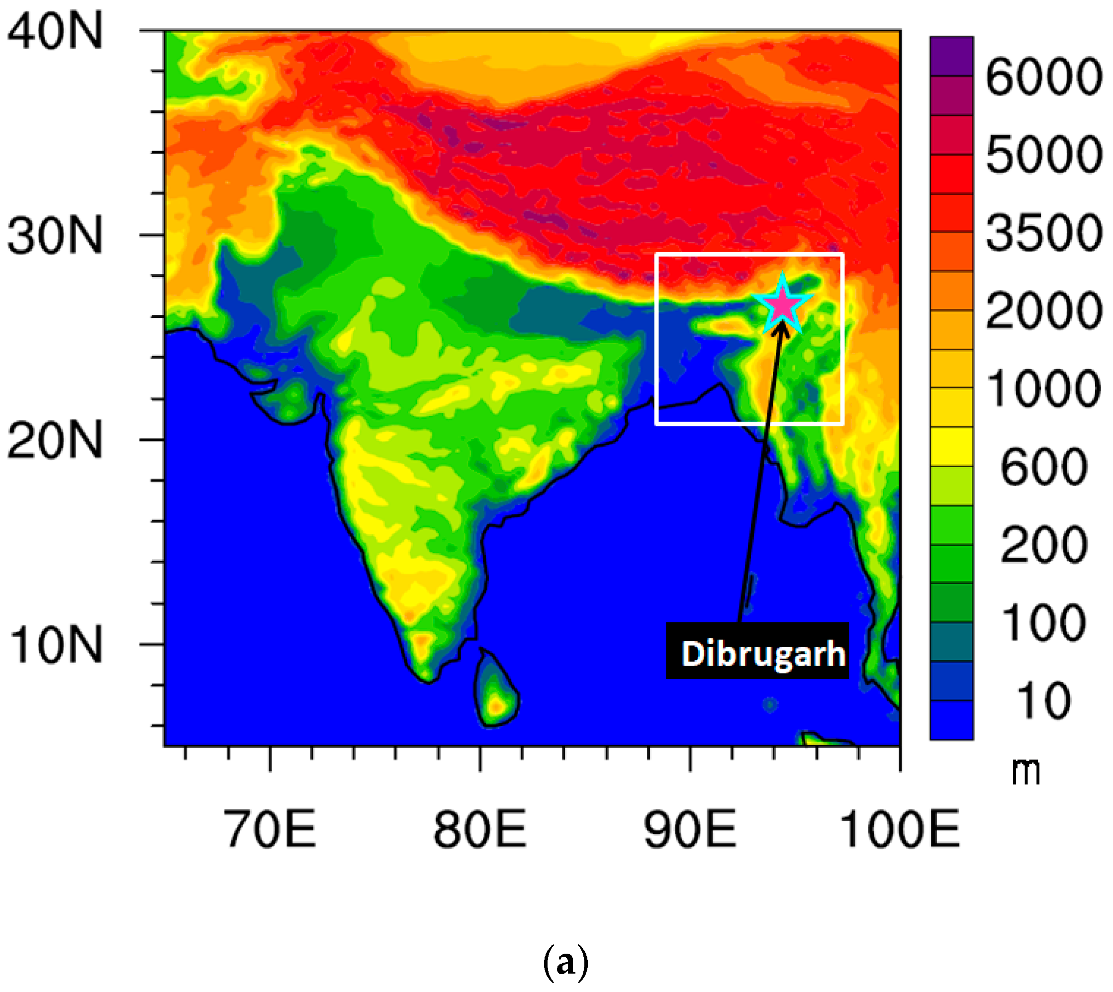
2. Site Description: North-Eastern India

The Eastern Himalayas including North-Eastern India (22–30° N, 88–98° E) possesses a unique topography (Figure 1a,b). The presence of hills, plateaus, and mountains around the north-east region keeps the rain-bearing monsoon winds in the area and hence influence the climate of this region [34,37]. North-Eastern India is characterized by rich biodiversity, heavy precipitation, and high seismicity [41].

The wide variety of weather and climate and being one of the highest rainfall-receiving regions on the planet makes it an important site from the meteorological perspective [34,41]. The study location, Dibrugarh, is (27.47° N, 94.89° E; 111 m amsl) (Figure 1a) situated along the bank of the river Brahmaputra and covered with dense vegetation. According to the 2011 census, the population density of Dibrugarh is 393 people per square kilometer, which is far less than in most Indian metropolis including Delhi (11,297 people per square kilometer) and Mumbai (19,652 people per square kilometer). Dibrugarh is the gateway to the tea-producing areas of Assam and is very rich in minerals and has large deposits of crude oil and coal [15]. Petroleum, petrochemicals products, and natural gas production play an important role in the economy and industrial development of the district as well as the state. The oil, natural gas fields, chemical and fertilizer industries, tea processing factories and coal mines are scattered within a 50–80 km area, primarily in the north-east, south-east and south-west of the monitoring site. There are many brick kilns in and around the observational site (Figure 1b). These are the major sources that emit gases like SO₂, CO, O₃, NO_x, etc. In addition, vehicular emissions and seasonal biomass burning, forest fires and crop residue burning prevailing nearby the hilly areas are possible sources of trace gases along with aerosols [38,42] around this location. More details on the measurement site Dibrugarh is available elsewhere [34,38,42].

3. Data and Methodology

3.1. Observation

3.1.1. Meteorological Data

Meteorological data over Dibrugarh were obtained from the Global Historical Climate Network and provided by the NOAA National Climate Data Center (NCDC; http://www.ncdc.noaa.gov/). The climate data center collect the data from a wide variety of sources, including weather satellites, radar, automated airport weather stations, National Weather Service (NWS), aircraft, ships, radiosonde, wind profilers, etc. The NOAA NCDC provides a historical perspective on climate/weather observations over 100 of years which were vital to studies on global climate change, the greenhouse effect, and other environmental issues.

3.1.2. Pollutant Data

CO, SO₂, O_3, and NO_x concentrations are collected at intervals of 5 min using CO (T300), SO₂ (T100), O₃ (T400) and NO_x (T200) Teledyne API analyzers (A Teledyne Technologies Company, 16830 Chestnut Street City of Industry, CA 91748, USA), respectively. The CO analyzer operates on the principle of infrared absorption at 4.7 μm, the vibrational rotation band of CO. This instrument has a lowest detection limit of 0.04 ppm, a precision of 0.5% and a response time of 10s. The SO₂ analyzer is based on the principle of fluorescence that occurs when SO₂ is excited by the ultraviolet light of wavelengths in the range 190–230 nm. The instrument has a lowest detection limit of 0.4 ppb, a precision of 0.5% and a response time of 20 s. The O₃ Analyzer (T400) is based on the well-established technique of absorption of ultraviolet light at 254 nm. The NO_x analyzer works on the basis of the chemiluminescence effect produced by the oxidation of NO by O₃ molecules, which peaks at 630 nm. NO₂ is measured by converting it into NO using the thermal conversion method (molybdenum convertor). Once the NO₂ in the sample gas has been converted to NO, it undergoes the chemiluminescence reaction, hence the analyzer can measure the total NO_x (NO + NO₂). Finally, the NO₂ concentration is not directly measured but calculated by subtracting the known NO content of the sample gas from the known NO_x content. The lower detection limits for the O₃ and NO_x analyzers are 0.6 ppb and 0.4 ppb and both have measurement precision of 0.5 %, and their response times are 10 s and 20 s. Further details of the instrument can be found in Bhuyan et al. [15] and references therein. These measurements are available since 2011 over the measurement location, which is reported earlier by Bhuyan et al. [15], Bharali et al. [37] and Pathak et al. [38] etc.

The BC data are obtained using an aethalometer, which measures attenuation of a light beam at seven different wavelengths (370, 470, 520, 590, 660, 880 and 950 nm), transmitted through the aerosols deposited continuously on a quartz fiber filter tape [43], at a temporal resolution of 5 min and flow rate of 3 L/min. Observations at the 880 nm wavelength are considered standard for BC measurement as it is the principal absorber of light at this wavelength, whereas other aerosol components have negligible absorption. However, this kind of filter based absorption techniques suffer from various errors. For example, the attenuation of light is enhanced by multiple scattering effects in the filter tape, thereby increasing the optical path. This multiple scattering effect is corrected by the Weingartner correction factor “C”. Moreover, the attenuation is gradually increased by light absorbing particles accumulating on the filter tape reducing the path length. This is known as shadowing effects and is corrected by Weingartner correction factor “R” [44,45]. For the measurements over Dibrugarh “C” value is assumed to be equal to 2.14 and “R” is assumed to be 1 [42,45]. More details on BC evolution, deposition, transportation, etc., over Dibrugarh are available elsewhere [34,42].

3.1.3. Fire Radiative Power (FRP) Data

Fire radiative power (FRP) data obtained from MODIS instruments onboard the Aqua and Terra satellites are used in this study to elucidate the peak BB period (March 2013). It is a multi-spectral sensor with 36 spectral bands from 0.4 to 14.2 µm. The two MODIS Sun-synchronous, polar-orbiting satellites Terra and Aqua pass over the equator at approximately 10:30 a.m. (Terra) and 1:30 p.m. (Aqua) with a revisit time of 1–2 days. The MODIS sensor onboard on Terra and Aqua satellite detects fire pixels and estimates FRP, the rate of fire energy released per unit time, globally on a daily basis. FRP is a suitable parameter for estimating the contribution of biomass burning to local and global carbon budgets. The satellite detects fire pixels and estimates FRP, the rate of fire energy released per unit time, globally on a daily basis. The daily values of fire count data over the study location are classified into medium confidence (30–80%) and high-confidence (80–100%). The major fires (high FRP) are indicated in both moderate- and high-confidence data. The details about the fire detection algorithm and FRP data are described in Giglio et al. [46]. The gridded active fire count data are generated from MODIS at 1° spatial resolution for the time period. The MODIS FRP data was used in a previous study over the same study location [34,47].

3.2. Models/Reanalysis Data

3.2.1. Weather Research and Forecasting Model Coupled with Chemistry (WRF-Chem) Model

In this study, we used the WRF-Chem (version 3.8.1) [48,49] model at a spatial resolution of 25 km with 40 vertical levels to simulate the meteorological parameters and air pollutant over Dibrugarh. The simulation domain is defined on the Mercator projection. The meteorological data are taken from the National Centers for Environmental Prediction Final Analysis (NCEP FNL from GFS ds083.2) (http://rda.ucar.edu/datasets/ds083.2/) with a spatial resolution of 1°, available every 6 h, to provide the initial and boundary conditions for the meteorological fields. Biogenic emissions of trace species are calculated online using the Model of Emissions of Gases and Aerosols from Nature (MEGAN). Anthropogenic emissions are taken from EDGAR-HTAPV2. Emissions from biomass burning are provided to the model via the Fire Inventory from NCAR version-1(FINNv1) [50]. Parameterizations used in this model study are provided in

Table 1. Parameters used in WRF-Chem model simulation. (WRF-Chem: Weather Research and Forecasting model coupled with chemistry).

Parameterization	Scheme	Reference
Bulk microphysical parameterization	Thompson scheme	[51]
Convective parameterization	Kain–Fritsch Scheme	[52]
Planetary boundary layer (PBL)	Yonsei University Scheme	[53]
Shortwave radiation physics	Dudhia Shortwave Scheme	[54]
Longwave radiation physics	RRTM Longwave Scheme	[55]
Photolysis	Madronich fast-Ultraviolet-Visible Model (F-TUV)	[56]

.

3.2.2. WRF-STEM Model

Version 3.5.1 of the WRF model [49] generated the required meteorological variables. The simulation domain is defined on the Mercator projection. The model domain is centered at 24.94° N and 82.55° E and covered the South and East Asian region with a spatial resolution of 25 km with 40 vertical levels. Similar to WRF-Chem, meteorological static input data are taken from the NCEP FNL with a spatial resolution of 1°, available every 6 h, to provide the initial and lateral boundary conditions for the meteorological fields. The parameterization schemes used in Table 1 are the same for the WRF-STEM model except for microphysics. The WSM3 microphysics scheme is used in this study.

The STEM has been used extensively in various field campaigns such as the Intercontinental Chemical Transport Experiment–Phase B (INTEX-B) [57,58] and TRACE-P/ACE-ASIA over East Asia [24]. The tracer version of the STEM model provides the mass concentration of sulfate, BC (hydrophobic and hydrophilic), OC (hydrophobic and hydrophilic), dust (fine and coarse) and sea salt (fine and coarse) aerosols. The tracer version of the STEM model employs simple decay rates for most of the primary species with no chemical production or loss but includes wet scavenging and dry deposition [59]. In addition, region-tagged CO tracers help to estimate the contributions from different geographic areas.

3.2.3. Emission Inventories

The emissions data available from different sectors such as energy, industry, residential, ground transport, ships, and agriculture are combined and then mapped on the WRF-STEM/Chem grids. For both WRF-STEM and WRF-Chem models, anthropogenic emissions of CH₄, CO, NO_x, SO₂, NMVOCs, NH₃, PM, BC, and OC are taken from the Emission Database for Global Atmospheric Research(EDGAR)-Hemispheric Transport Air Pollution version 2 (HTAPv2) emission inventory (http://edgar.jrc.ec.europa.eu/htap_v2) for the year 2010. Detailed information on the HTAP inventory can be found in Janssens-Maenhout et al. [60].

Fire INventory from NCAR (FINN), version 1 emissions data [61] are based on Rapid Response Moderate Resolution Imaging Spectroradiometer (MODIS) fire counts (NASA FIRMS Active Fire Data) developed specifically for modeling atmospheric chemistry and air quality. FINN provides global daily estimates of trace gases, including greenhouse gases (GHGs), CO, NOx, VOCs, SO₂ and NH₃. It also includes particle emissions from open burning of biomass (including wildfire, agricultural fires and prescribed burning which does not include biofuel use and trash burning) at 1 km resolution for use in regional and global chemical transport models [50]. Fire detections with low confidence (<20%) are removed. Uncertainties in the emission estimates may possibly arise from the use of fire hotspots, assumption of area burned, land cover maps, biomass consumption estimates, and emission factors. FINN fire product is used in WRF-STEM/Chem simulation.

3.2.4. HYbrid Single-Particle Lagrangian Integrated Trajectory (HYSPLIT) Model:

The HYbrid Single-Particle Lagrangian Integrated Trajectory (HYSPLIT) model, developed by the National Oceanic and Atmospheric Administration (NOAA) is used in the present study to depict the motion of the air parcel. The HYSPLIT model’s cluster analysis algorithm groups trajectories by minimizing the spatial variability between trajectories within some defined number of clusters [62]. In order to delineate the distinct mean pathways of the trajectories, the cluster analysis has been carried out by using Ward’s hierarchical method [63] to form the clusters by combining the nearest trajectories. In this study, we used three clusters which are formed by combining similar trajectories in terms of air mass movement to identify the dominant transportation pathways [64]. The isentropic back-trajectories are computed at 500 m above ground level (AGL) to identify the source regions. The model calculations are based on the Global Data Assimilation System (GDAS) meteorological field produced by NCEP Reanalysis data, with a horizontal resolution of 1° × 1°.

3.2.5. Copernicus Atmosphere Monitoring Service (CAMS)

CAMS provides a recent global model and reanalysis data set of atmospheric composition. It uses the four-dimensional variational (4D-VAR) data assimilation technique to combine satellite observations with chemistry-aerosol modeling to obtain the mass mixing ratios of atmospheric trace gases and aerosols [65]. The CAMS global model (Near-Real-Time) service provides daily analyses and forecasts of reactive trace gases, GHGs, and aerosol concentrations. The analyses are available at 6-hourly intervals at different spatial resolutions. In our study, we used CAMS model meteorological (temperature, relative humidity, wind speed, and wind direction) variables and air pollutants (CO, BC, SO₂, and O₃) datasets at a horizontal resolution of 0.25° × 0.25° from December 2012 to November 2013 (https://apps.ecmwf.int/datasets/data/cams-nrealtime/levtype=sfc/).

3.2.6. Modern-Era Retrospective Analysis for Research and Applications, Version 2 (MERRA2)

MERRA2 is a global reanalysis dataset produced by NASA Global Modeling and Assimilation Office (GMAO), using Goddard Earth Observing System Model, version 5 (GEOS-5) [66,67]. The GEOS-5 model coupled with the Goddard Chemistry Aerosol Radiation and Transport model (GOCART) aerosol module and simulates five types of bulk aerosols [68,69]. The model spatial resolution is 0.5° latitude × 0.625° longitudes respectively, with 72 hybrid-eta layers from the surface through 0.01 hPa. This provides regularly-gridded, homogeneous documents of the global atmosphere that integrates additional aspects of the climate system including trace gas constituents, land surface image, and cryospheric processes. In this study, the daily surface O₃ data over Dibrugarh are taken from MERRA2 assimilated ozone data product, which is produced at NASA’s GMAO from 1980 to the present [70]. From January 1980 to September 2004 the retrieved partial column ozone is assimilated from a series of Solar Backscatter Ultraviolet Radiometer (SBUV) instruments onboard on NASA and NOAA satellites. After October 2004 MERRA2 assimilates O₃ profiles retrieved from the Microwave Limb Sounder (MLS) and total column ozone from the Ozone Monitoring Instrument (OMI) on NASA’s EOS Aura satellite [70]. In addition MERRA2 variables such as OC, BC, Sea salt, dust, sulfate, SO₂ and CO are derived from Goddard Chemistry, Aerosol, Radiation, and Transport model (GOCART) integrated into the Goddard Earth Observing System Model, Version 5 (GEOS-5) data assimilation System [69]. The data are downloaded from (https://disc.gsfc.nasa.gov/datasets and https://goldsmr5.gesdisc.eosdis.nasa.gov/data/MERRA2/ M2I3NVCHM.5.12.4/2013/11/ (last accessed on September 2018).

3.3. Methodology

Two sets of numerical simulations are performed using WRF coupled with chemistry (WRF-Chem) and Sulfur Transport and dEposition Model (WRF-STEM) at a horizontal resolution of 25 km covering the South Asian domain. We have used two different versions of the WRF (3.5.1 and 3.8.1) model to evaluate the intra-model variability in simulating the meteorological variables. The simulations are performed from December 2012 to November 2013 because this period is free from natural phenomenon like El Niño and La Niña, which play a significant role in the variations of global wind, temperature and weather patterns. In addition, there are lesser data gaps in simultaneous measurements of various trace gases of interest over Dibrugarh in this year. Further, CAMS model and MERRA2 reanalysis data are used along with in-situ pollutants and meteorological variables to understand and evaluate WRF-Chem and WRF-STEM model performance over Dibrugarh. In this study, we used WRF-STEM region-tagged carbon monoxide (CO) to identify sources and regions [57]. The CO contribution from different sources is calculated by breaking the CO emission inventory into the anthropogenic and biomass burning components. Anthropogenic emission is further broken down into several geographic regions.

4. Results and Discussion

Surface measurements, models (WRF-Chem, WRF-STEM and CAMS) and reanalysis (MERRA2) datasets are used to comprehend the meteorological condition and air quality scenario over Dibrugarh. The WRF-Chem model is extensively used in weather/climate research by the global community. Several versions of WRF model simulation have already been validated over the Indian/South Asian domain [7,71,72,73,74]. As such, use of this different version of the WRF model over the less explored Eastern Himalayan foothills region is beneficial for intra-model and inter-model evaluation of meteorological drivers and air pollutants over the complex terrain. The WRF-STEM CO tracer and HYSPLIT model classify different geographical regions affecting the air quality over Dibrugarh. The WRF-STEM model used in the present study has already been validated over the complex terrain in Central and Western Himalayan region [75,76]. In contrast to WRF-Chem and WRF-STEM, HYSPLIT is a computationally inexpensive and easily accessible model for identification of concentration pathways. MERRA2 with a rich database obtained using advanced data assimilation techniques is being used extensively by researchers. CAMS gives the latest global atmospheric composition data at a finer resolution as described in methodology section.

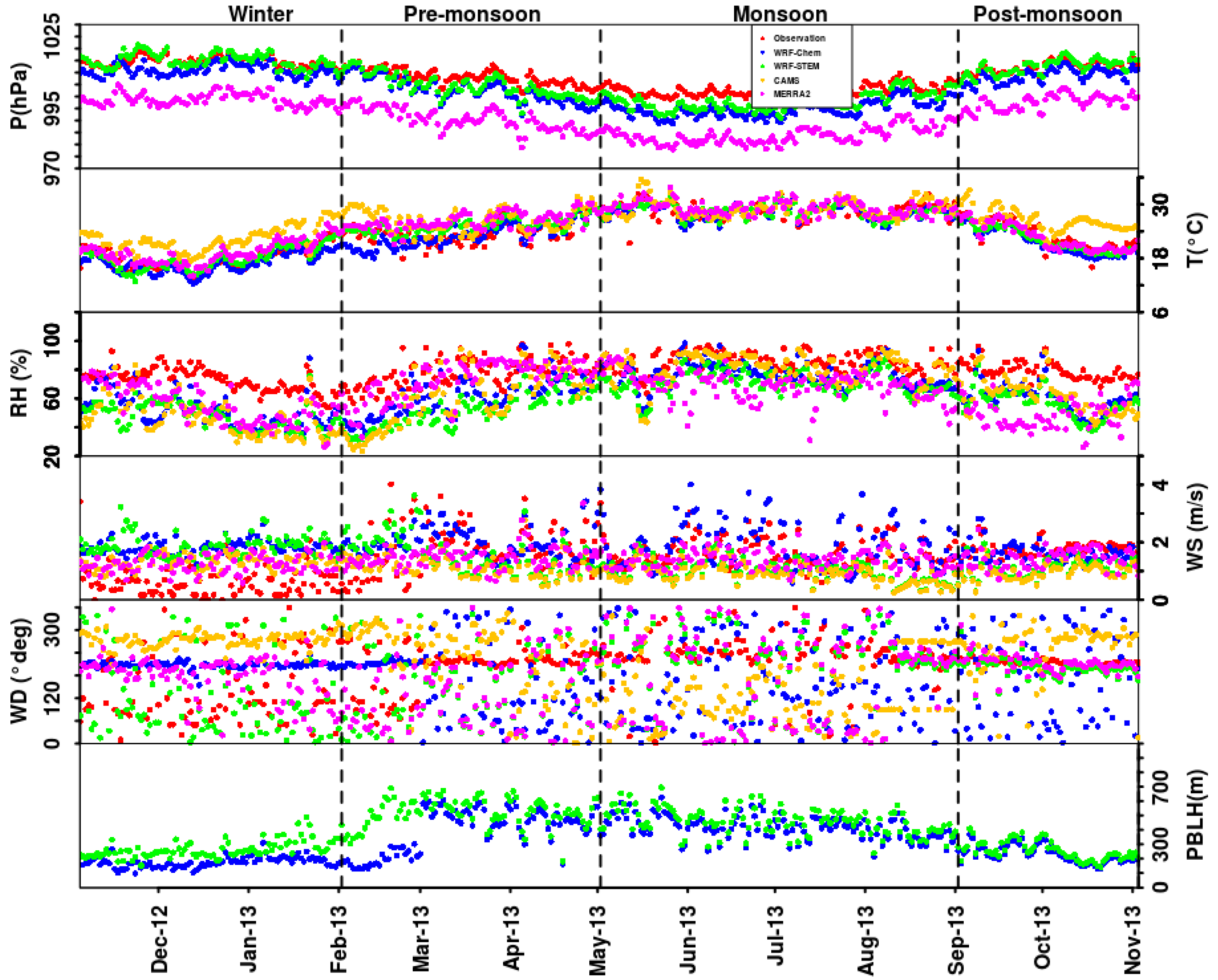
4.1. Evaluation of Surface Meteorology

North-Eastern India including Dibrugarh is subject to a humid subtropical climate characterized by hot and humid summers, and cool winters [15]. The winter season (December–February) is associated with fog and haze, while the pre-monsoon (March–May) is characterized by high wind-speed [37,77]. The monsoon season (June–September) exhibits mostly cloudy and rainy days, which abruptly decrease in the post-monsoon (October–November) period.

The seasonal variability of surface measured pressure (P) is well captured by the models and reanalysis data sets (Figure 2) except MERRA2 which underestimates P by ~10 hPa. Both observation and models show higher values of P during winter and post-monsoon than in pre-monsoon and monsoon seasons. The high P is associated with cold air, which is denser than warm air and has the tendency to sink due to gravity. Whereas, low value of P is attributed to intense solar insolation, as earth’s surface heats the air in contact with it, the warm air rises, there is less air near the surface, with a consequent decrease in surface P. Atmospheric temperature exhibits an important role in atmospheric chemistry as it controls the rate of chemical reactions and helps in gas-particles conversion [78]. In contrast to P, the surface temperature (T) is less in winter and post-monsoon compared to rest of the seasons, monsoon being the hottest season over Dibrugarh. WRF-Chem, WRF-STEM and MERRA2 show good performance relative to CAMS (overestimate by ~1–3 °C) in simulating daily T during winter and post-monsoon seasons. While all models and reanalysis products capture the seasonal variation of relative humidity (RH) relatively well, however the magnitude of actual measured RH values are underestimated in all seasons except in monsoon. The surface measured RH ≥ 90%, particularly in the monsoon are associated with saturation [79], which causes heavy rainfall over a region [80]. Under low RH condition, the significant impact of regional transportation, local emissions, and physicochemical formation jointly dominates the concentration of atmospheric particles [81]. Thus, an increase in the value of RH is favorable for the formation of particles from the liquid-phase, heterogeneous reactions and the hygroscopic growth processes [75]. High T, low wind and RH play a significant role in the enrichment of regional pollution.

Wind speed (WS) and wind direction (WD) control the horizontal transport and thereby the spatial distribution of pollutants. WS is particularly an important parameter as it influences the volume of air by means of dilution or dispersion, determines the transport time between sources and receptor locations, and also controls the emission of pollutants. Both the WRF-Chem and WRF-STEM models overestimate the WS in all seasons with the highest bias in winter (

Table 2. Statistics between observed and models/reanalysis meteorological parameters. (WRF-Chem: Weather Research and Forecasting model coupled with chemistry, WRF-STEM: WRF coupled with Sulfur Transport dEposition Model, CAMS: Copernicus Atmosphere Monitoring Service, MERRA2: Modern-Era Retrospective Analysis for Research and Applications, Version 2).

Temporal Scale	Statistics	Pressure (hPa)			Temperature (°C)				RH (%)				WS (m/s)
	Observation vs Models/Reanalysis	WRF-Chem	WRF-STEM	MERRA2	WRF-Chem	WRF-STEM	CAMS	MERRA2	WRF-Chem	WRF-STEM	CAMS	MERRA2	WRF-Chem	WRF-STEM	CAMS	MERRA2
Annual	Mean_obs	1008.61	1008.55	1008.61	23.86	23.9	23.85	23.86	81.17	81.16	80.76	80.79	1.35	1.35	1.36	1.35
	Mean_Model/Reanalysis	994.77	997.14	986.08	23.07	24.08	26.31	24.9	63.72	57.98	64.06	62.97	1.84	1.81	1.08	1.38
	Bias	13.84	11.42	22.52	0.79	−0.18	−2.47	−1.04	17.46	23.18	16.69	17.82	−0.48	−0.45	0.27	−0.03
	Normalized mean bias	0.01	0.01	0.02	0.03	−0.01	−0.1	−0.04	−1.24	−0.95	−1.62	−1.17	−0.36	−0.34	0.2	−0.02
	MAE	13.84	11.42	22.52	1.45	1.29	2.75	1.58	17.68	23.18	17.46	19.23	0.85	0.81	0.85	0.71
	RMSE	13.89	11.48	22.55	1.81	1.71	3.36	2.1	25.68	29.7	25.26	26.84	1.01	0.97	1.03	0.86
	Correlation Coefficient	0.98	0.98	0.98	0.94	0.93	0.89	0.92	0.4	0.4	0.46	0.23	0.37	0.45	0.29	0.39
Winter	Mean bias	14.25	11.14	23.47	1.14	0.33	−0.15	−1.25	21.74	26.03	1.24	17.62	−1.21	−1.03	0.02	−0.62
Pre-monsoon		13.65	12.27	22.88	0.66	−1.47	−2.66	−2.46	16.62	26.13	16.55	5.66	−0.15	−0.18	0.71	0.38
Monsoon		13.99	11.53	22.10	0.32	0.16	−0.27	−0.49	12.29	17.29	8.76	20.09	−0.10	−0.10	0.80	0.33
Post-monsoon		13.46	10.54	21.83	1.44	0.89	−3.51	0.31	20.80	24.59	19.40	32.21	−0.70	−0.70	−0.07	−0.52
Winter	Correlation coefficient	0.64	0.93	0.65	0.87	0.88	−0.20	0.88	0.50	0.71	0.05	0.59	0.06	0.35	0.82	0.12
Pre-monsoon		0.96	0.95	0.98	0.71	0.75	0.73	0.66	0.78	0.74	0.82	0.56	0.42	0.44	0.21	0.44
Monsoon		0.94	0.92	0.94	0.59	0.55	0.66	0.57	0.29	0.22	0.26	0.08	0.47	0.47	0.28	0.49
Post-monsoon		0.97	0.97	0.98	0.92	0.92	0.74	0.92	0.17	0.10	0.18	-0.05	0.39	0.39	−0.16	0.09

). Whereas CAMS underestimates in all season except post-monsoon and MERRA2 underestimates in pre-monsoon and monsoon seasons. The under and overestimation of measured WS by the models and reanalysis data is attributed to the parameterization adopted in the model and temporal and spatial grids of the reanalysis data, which are too coarse to identify some of the major events and stronger winds [82]. In pre-monsoon season, the surface measured wind is predominantly blowing from the south-west (i.e., 180°–210°) direction. In order to better understand the direction of the wind, NOAA NCEP HYSPLIT model back trajectory analysis data will be presented in a subsequent section of this study. The simulated PBLH for two sets of WRF simulations shows lower values in winter and post-monsoon compared to those in pre-monsoon and monsoon. Estimating PBLH and RH values with less uncertainty is essential for air quality assessment over a region [38,81]. The PBLH plays a crucial role in pollutant dilution and dispersion and hence governs the surface level concentrations of atmospheric constituents by virtue of vertical mixing [83]. The models and reanalysis RH underestimated the measured RH in all seasons (with maximum bias ~26.13% for models in pre-monsoon season and ~32.21% for reanalysis in post-monsoon season) (Table 2).

This underestimation of RH may affect the convective processes like PBLH. To reduce the uncertainties in the model simulation, the quality of the input meteorological data like PBLH and RH datasets reportedly needs further improvement [84].

To quantify uncertainties in simulated meteorological variables, we perform statistical analyses such as model/reanalysis mean, observation mean, bias, root mean square error (RMSE), mean absolute error (MAE) and correlation coefficient (R) between observation and Models/Reanalysis data (Table 2). The RMSE and MAE are standard statistical parameters used to evaluate models performance for meteorology, as well as in air quality studies [85]. The correlation coefficient R is used to measure the strength of the linear relationship between observed and model-simulated variables. The seasonal and annual biases and correlation coefficient values presented in Table 2 are obtained by subtracting the model-simulated data set from the observation [86]. The data which are not available for particular measurement methods are not included in the table. The correlation between models and MERRA2 reanalysis for P is good. However, in the case of T the WRF-STEM, CAMS and MERRA2 overestimate the measured T by ~1–2 °C. WRF-Chem, WRF-STEM and MERRA2 overestimate and CAMS underestimates surface WS by ~0.4 m/s and 0.2 m/s, respectively. In addition, the simulated and reanalysis RH is underestimated by several magnitudes with mean biases of ~1.24–32.21% (Table 2). Both models and reanalysis data show small biases, MAE and RMSE for P and T values relative to RH and WS, indicate that the errors in simulated P and T are small [71,87], which is very important in air quality studies. The existing uncertainties in models and measurements are due to factors like assimilation method used in the reanalysis and model physical parameterizations which are responsible for both underestimation and overestimation of reanalysis pressure and temperature data [88]. On the other hand coarse spatial resolutions of a grid cell data used in the reanalysis database cause underestimation of meteorological variables like WS, RH, and T.

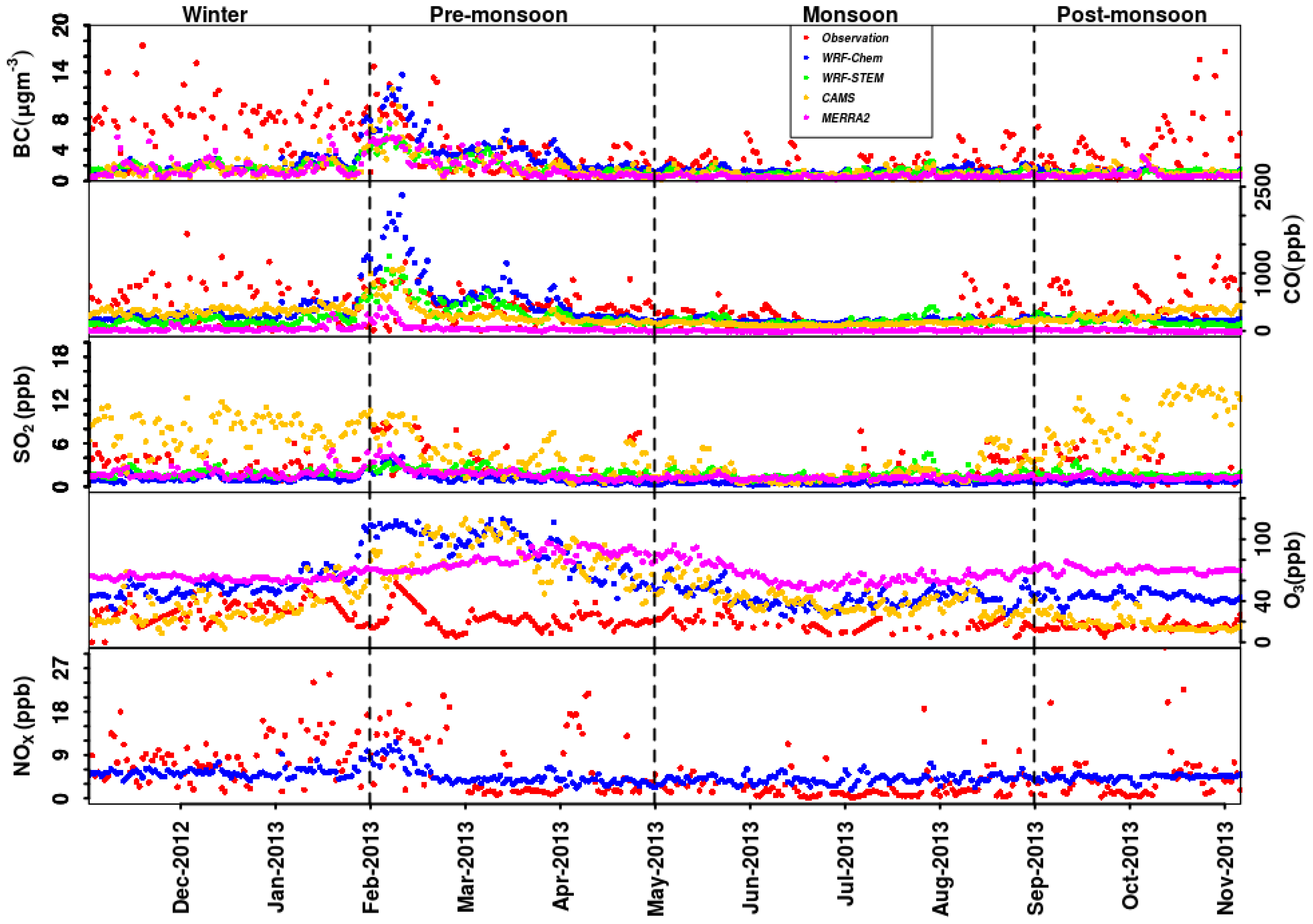
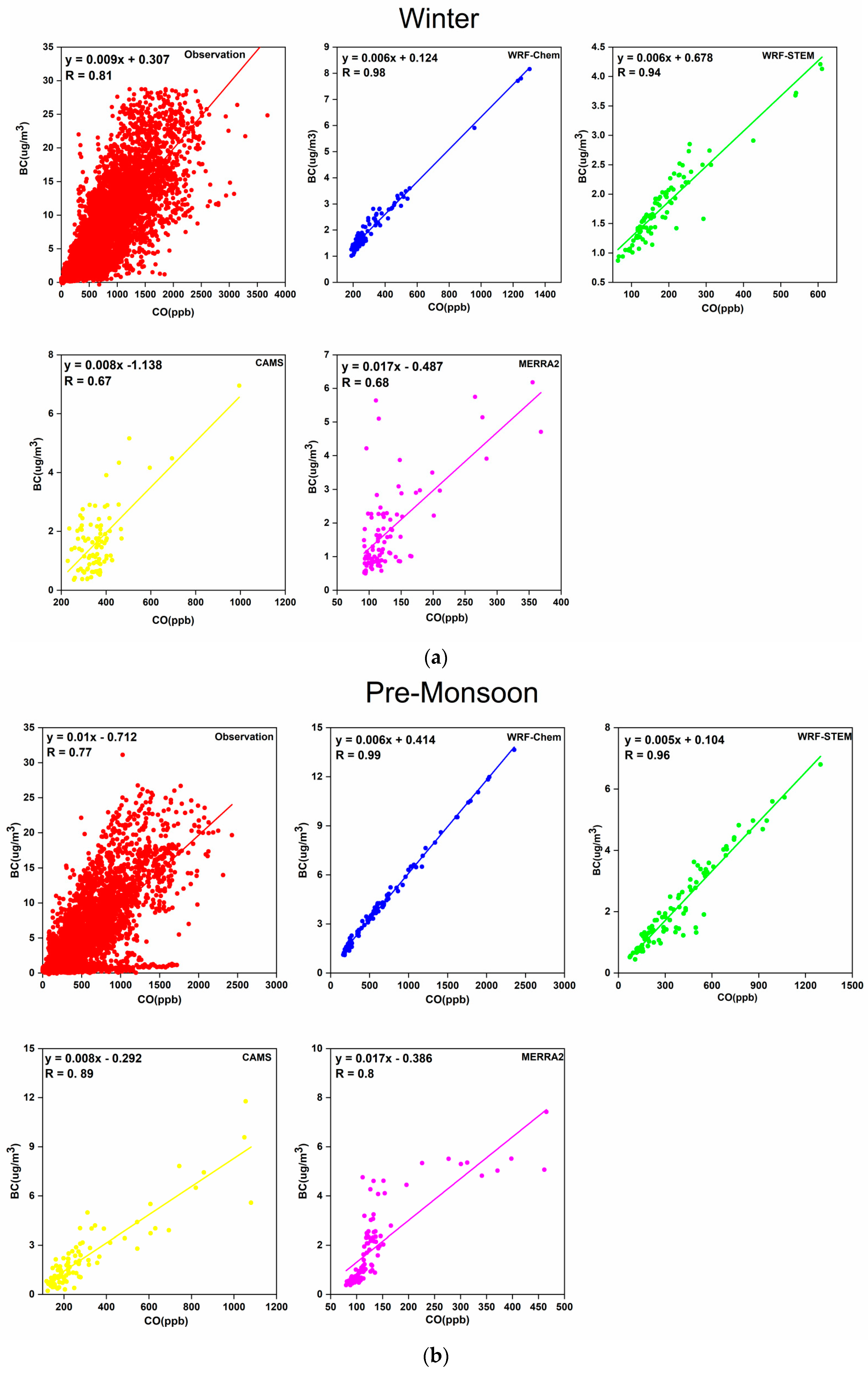
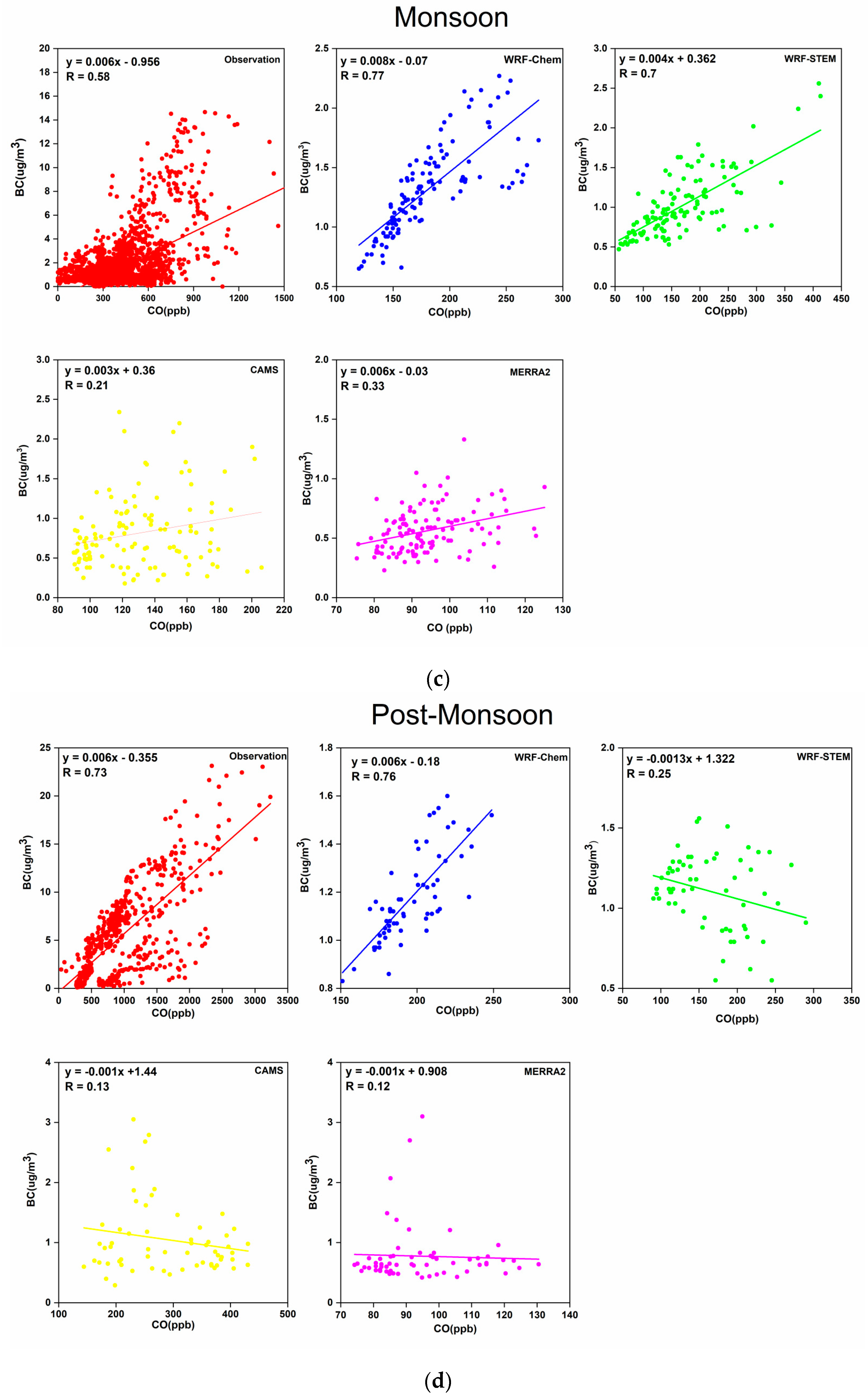
4.2. Evaluation of Surface Air Pollutants

The measured near-surface BC and CO concentrations are highest during winter whereas the model (WRF-Chem, WRF-STEM, CAMS) and reanalysis (MERRA2) data show highest values only in the pre-monsoon season (Figure 3). A similar result of high BC and CO concentrations in winter has been reported earlier over Dibrugarh by Pathak et al. [89]. The underestimation of models and MERRA2 BC and CO during wintertime is associated with biases in simulated surface winds over Dibrugarh. Figure 2 shows stagnation condition of observed WS during winter, while models show WS ~ 1–2 m/s. Further PBLH play a significant role in varying the concentration of pollutants over Dibrugarh during winter month. Likewise, local anthropogenic emissions, less precipitation/wet removal in winter leads to accumulation of pollutants resulting in higher concentration levels [38,42,89]. In addition, emission activities like trash/wood/biomass burning taking place at local scale mostly in the winter and pre-monsoon season are undetectable by the satellites and also are not incorporated properly in the emission inventory [74]. For example, the different inventories adopt different criteria for compiling data and have diverse resolutions and spatial disaggregation methods, etc. Emission inventories collect the activity data at the regional or national level and then spatially interpolated to generate data at local scale [90], which may lose some information about local scale emission. Similarly, several studies in South-Asia also found the limitation of the models in predicting the wintertime measured BC [81,91,92,93,94]. The possible causes of underestimation are boundary layer parameterization, coarse spatial resolution of the models and the emissions inventory used for the simulations [95,96]. RH also plays a significant role in varying the chemical composition of the atmosphere. Zhang et al. [97] reported that the concentrations of particulate matter, CO, SO₂, and NO₂ show positively correlated with RH in all seasons, especially in winter. Bharali et al. [73] have shown that change in aerosols is significantly associated with change in RH during wintertime. Furthermore, small to large-scale biomass burning (BB) activities, practices of shifting cultivation in the hills of North-Eastern states from November to March also contribute to higher BC as well as CO levels. An abrupt rise in BC and CO concentrations is identified in the pre-monsoon season from all models, reanalysis and measured data. The measured SO₂ does not show systematic temporal variation during the study period. CAMS SO₂ overestimates all other evaluations during all the seasons. During pre-monsoon season, surface observation, models and reanalysis data show a high concentration of O₃, due to abundant solar insolation available for photo-chemistry. However, the absolute magnitudes of the surface measured O₃ are overestimated by WRF-Chem, CAMS, and MERRA2 throughout the analysis period. The overestimation of modeled O₃ is attributed to the biases in simulated T, which may affect the gas phase chemistry by under/overestimating photochemical ozone production and affect the dry deposition of pollutants by reducing the strength of mixing within the boundary layer. The uncertainties in model simulated ozone precursors such as NO_x and CO also play significant role in altering the concentration of O₃. Besides these, underestimation of simulated and reanalysis RH may affect the concentrations of simulated pollutants. For example, a dry bias in the model will underestimate the concentrations of hydroxyl radicals, which will affect the concentrations of many VOCs and O₃. Furthermore, emission inventories used in the models simulation (EDGAR-HTAPv2 emission data for WRF-Chem/STEM and in CAMS, anthropogenic emissions are taken from MACCity (combined MACC and CityZEN projects) [98] also contribute uncertainties in the pollutants levels. A number of studies using different emissions inventories as model input found differences in surface O₃ concentrations levels [99,100]. For example the presence of NO_x and non-methane volatile organic compounds (NMVOCs) in the emission inventories is one of the factors for the uncertainties [101]. The NO₂ photolysis is an important source of tropospheric O₃, so any change in the amount of NO_x leads directly to the change in O₃ concentration. Likewise, O₃ is also produced as a result of a complex set of reactions involving VOC. Thus, increase or decrease of O₃ concentration depends on the ratio of NO_x and VOC over that region.

Bhuyan et al. [15] have carried out extensive work on surface O₃ over Dibrugarh based on surface observation data. They have shown that there exist a negative correlation between O₃ and NO_x, signifying that O₃ formation comes under VOC-limited (NO_x-saturated) regime over Dibrugarh. In the NO_x-saturated regime, with abundant NO_x, the rate of the OH + NO₂ termination reaction increases as NO_x increases, removing both HO_x and NO_x from the system, limiting OH–HO₂ cycling, thus decreasing the rate of O₃ formation [102].

In addition, chemical mechanism (MOZCART/tracer bulk aerosol scheme with parameterized sulfur chemistry) introduced in the models (WRF-Chem) also play significant role in simulating the actual magnitude of pollutants concentration. Sharma et al. [74] reported that over South Asia, WRF-Chem simulated daily average O₃ with MOZART chemical mechanism are higher compared to RADM2 chemical mechanism. For example, WRF-Chem simulated O₃ with the MOZART chemical mechanism shows greater value at Dibrugarh compared to RADM2 mechanism [90]. The differences in chemical mechanisms are mainly attributed to the additional chemical species and reactions in the model. The validation of NO_x with surface observation is difficult because of the short lifetime and large variability in the sources. WRF-Chem model has large uncertainties in simulating NO₂ due to uncertainties in emissions from biomass burning and anthropogenic NO_x emissions [71].

Similar to Table 2, the pollutants statistics are presented in

Table 3. Statistical evaluation between observed and models /reanalysis CO, BC, SO₂, O_3, and NO_x.

Statistics	CO (ppb)				BC (ug/m3)				SO2 (ppb)				O3 (ppb)			NOx (ppb)
Observation vs Models/Reanalysis	WRF-Chem	WRF-STEM	CAMS	MERRA2	WRF-Chem	WRF-STEM	CAMS	MERRA2	WRF-Chem	WRF-STEM	CAMS	MERRA2	WRF-Chem	CAMS	MERRA2	WRF-Chem
Mean_observation	423.61	423.61	423.61	423.61	4.24	4.24	4.24	4.24	3.42	3.42	3.42	3.42	22.08	22.08	22.08	5.67
	370.43	237.8	273.34	116.31	2.31	1.56	1.45	1.3	0.97	1.9	6.06	1.63	61.2	46.7	70.54	4.63
Mean_Model/Reanalysis
Bias	53.17	185.81	150.27	307.3	1.93	2.68	2.79	2.94	2.45	1.52	−2.64	1.79	−39.12	−24.61	−48.46	1.04
Normalized mean bias	0.13	0.44	0.36	0.73	0.46	0.63	0.66	0.69	0.72	0.45	−0.77	0.52	−1.77	−1.12	−2.19	0.22
MAE	325.03	293.2	274.12	338.21	2.87	3	3.11	3.2	2.53	1.96	3.49	2.08	39.13	27.69	48.46	3.96
RMSE	451.43	394.23	342.82	431.81	4.21	4.36	4.53	4.56	3.14	2.52	4.68	2.65	45.73	37.86	50.6	6.13

. The under-estimation of models/reanalysis CO, BC, SO₂, NO_x, and overestimation of O₃ is associated with the coarse spatial resolution of the models and satellite assimilation techniques as well as emission inventories used, which may not adequately capture the local scale emissions (trashing/wood burning to keep warm from chilled winter). Further, the uncertainties in the model simulation are associated with biases in simulating meteorological variables like T, RH, and WS, which affect the reaction rates, formation and loss processes as well as transportation, etc. For example, the moisture content in the atmosphere and the wind play a significant role in dispersion and dilution of the species, thereby changing the mixing ratios in the air over a region.

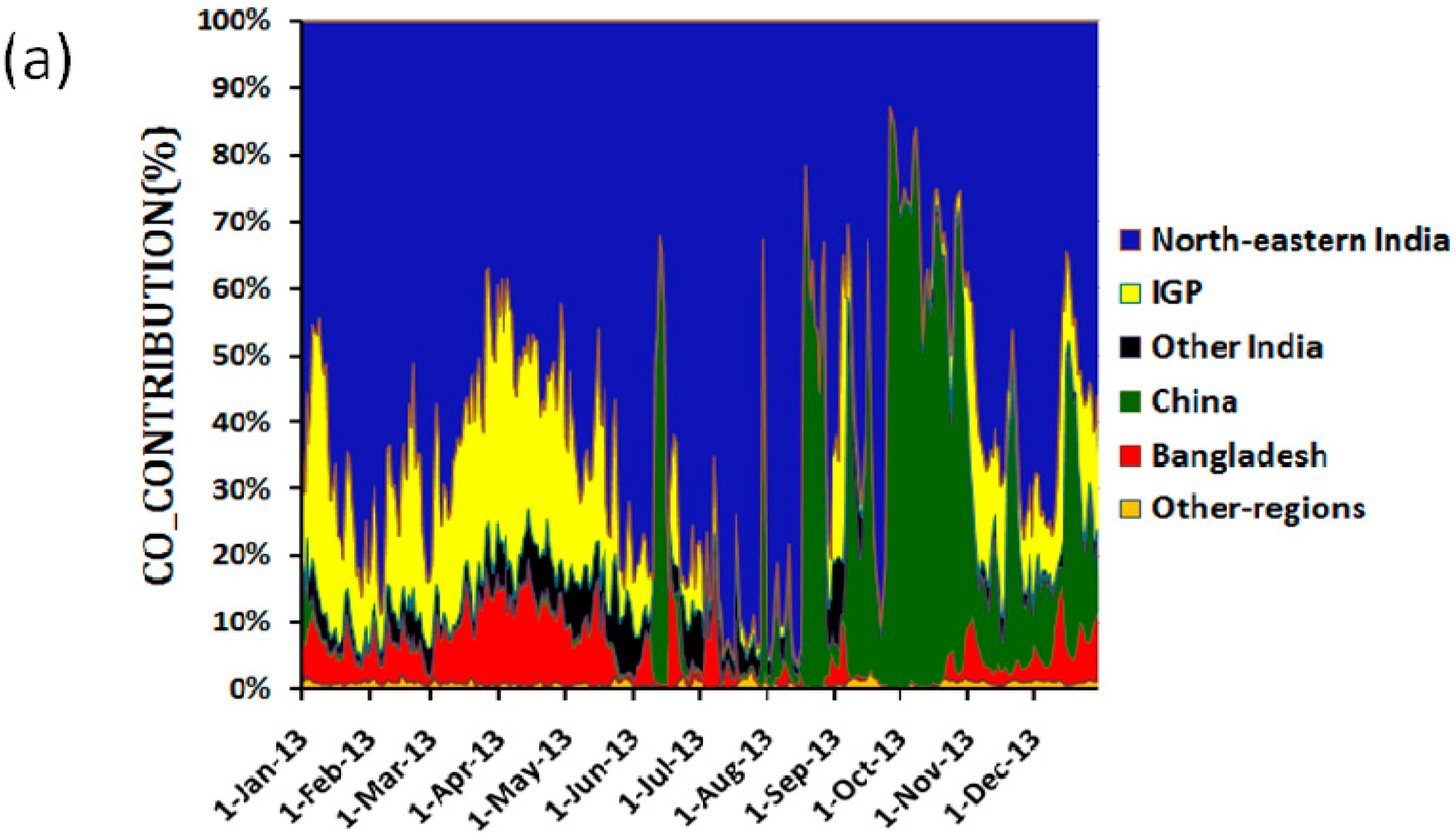
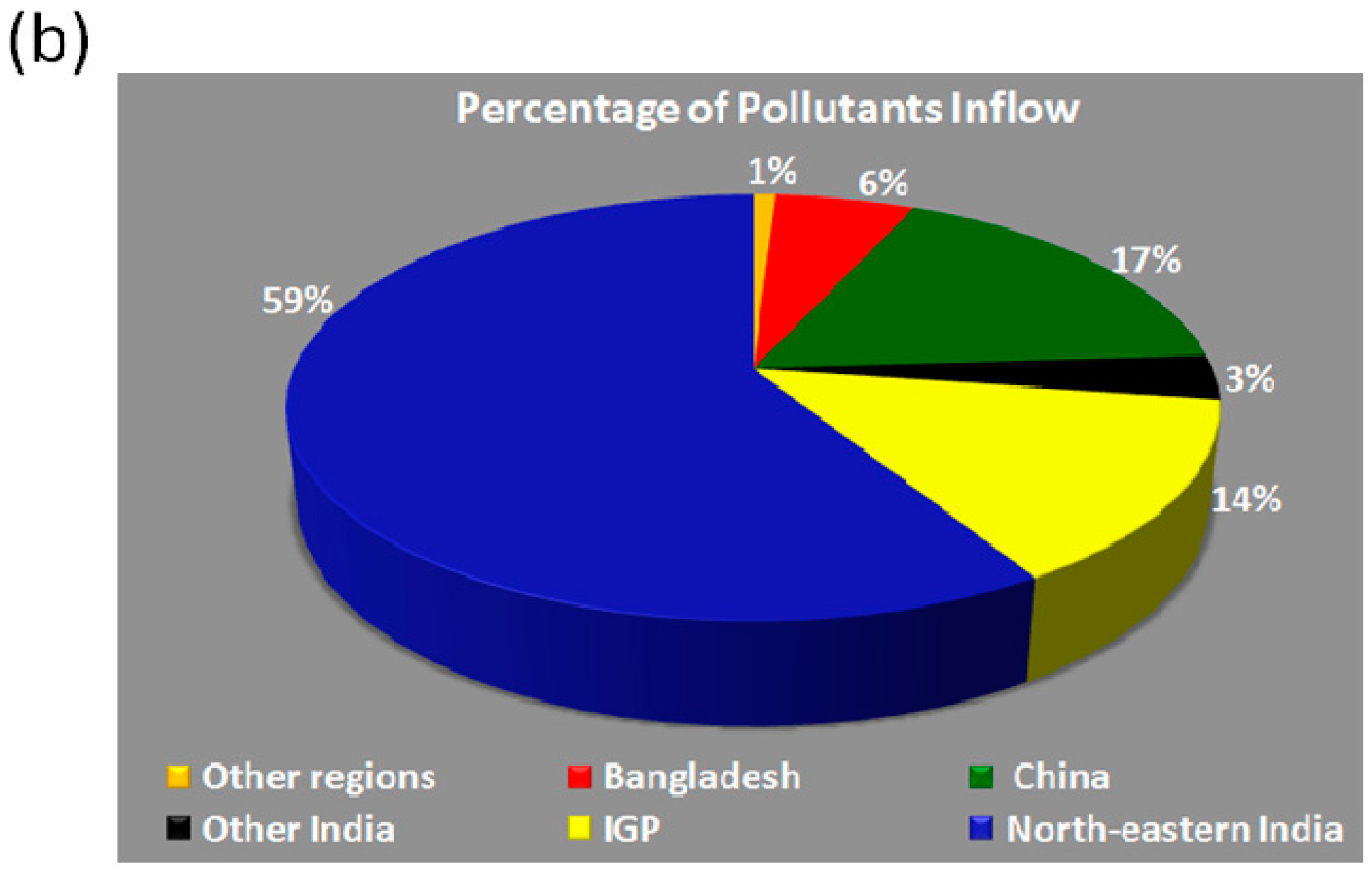
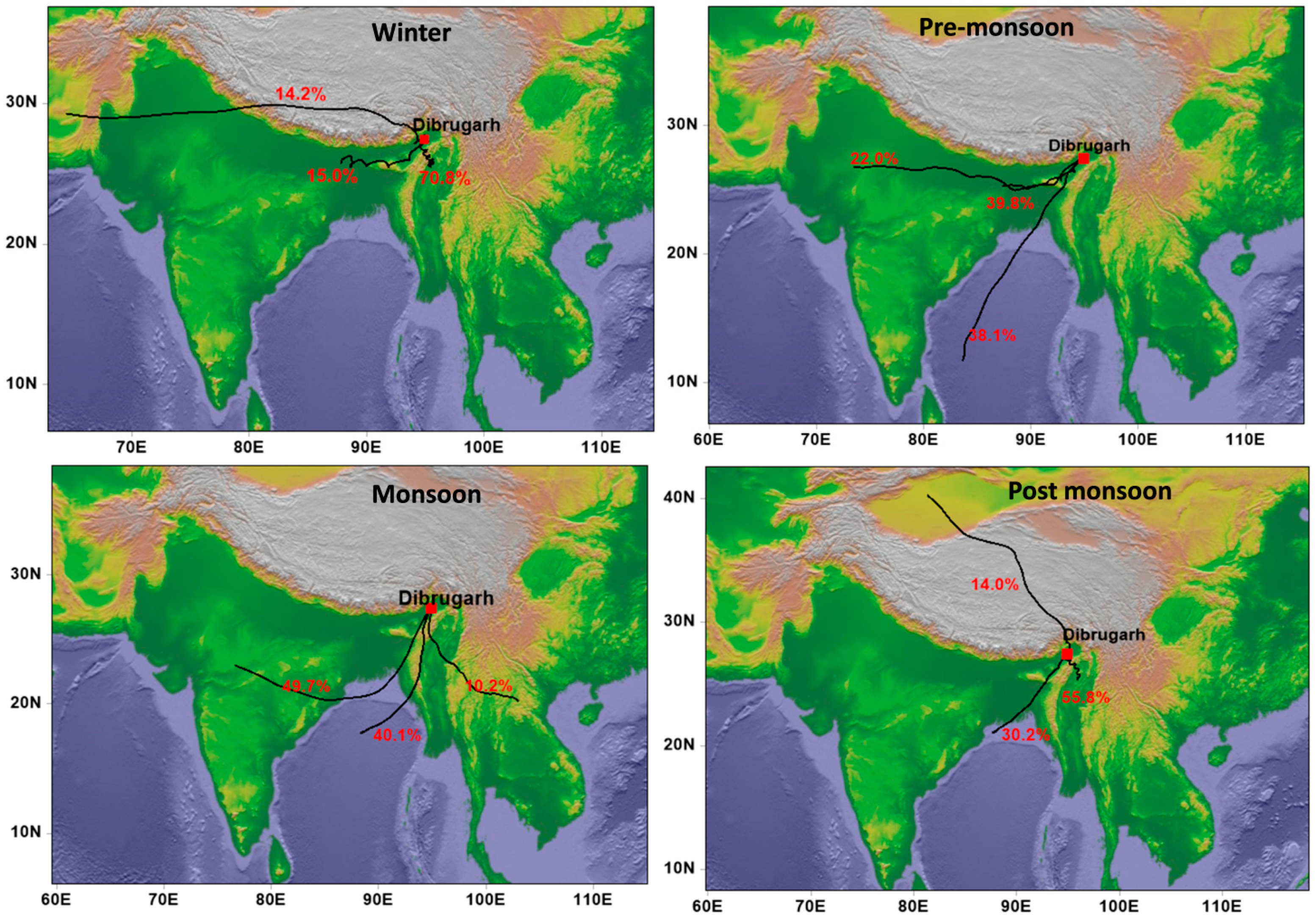
4.3. Delineation of Source Regions

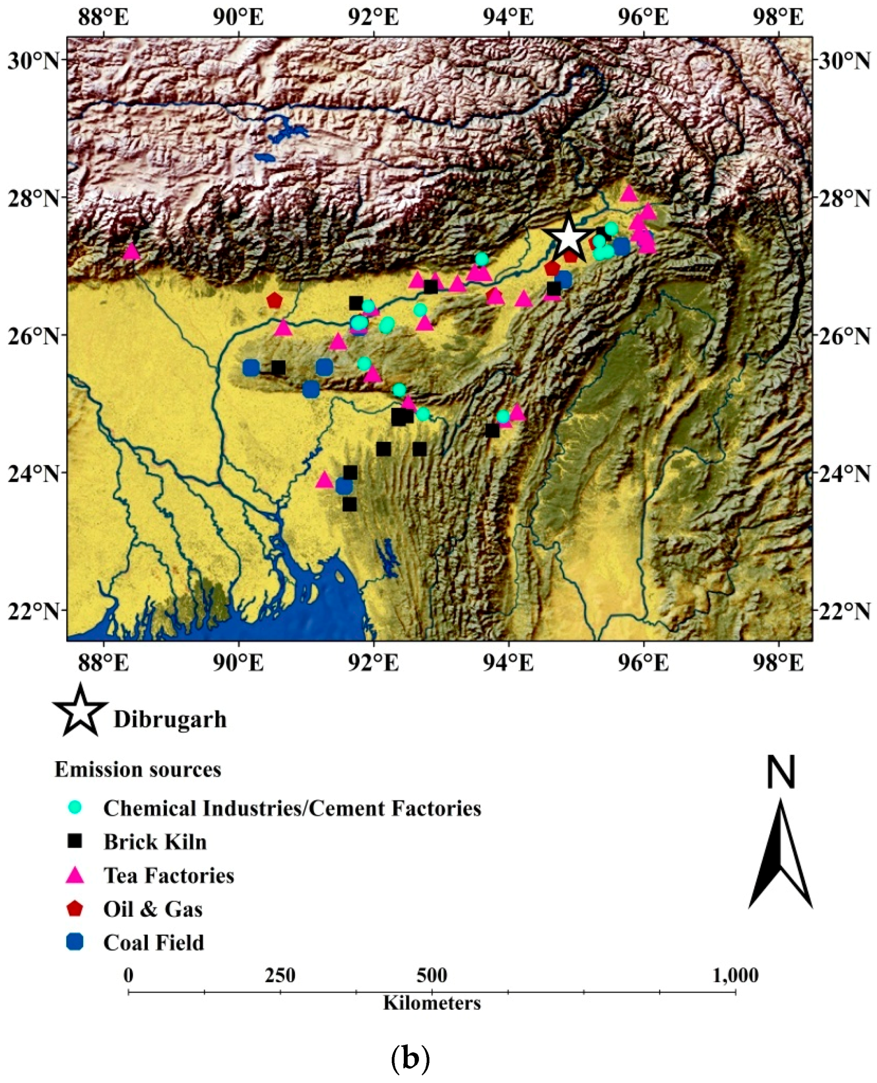
4.3.1. Local Sources

Species–species correlation analyses are useful for examining the relationship between species and hence to delineate the common spatio-temporal emission sources. Therefore, in this study, we illustrate the seasonal BC and CO correlation over Dibrugarh using surface observations, multiple models, and satellite assimilated data (Figure 4). In order to ascertain the atmospheric pollution picture over Dibrugarh, the measured BC and CO data available in 5 min intervals are used for calculating the correlation between them [38,84]. In doing so we get a better correlation between BC and CO than the daily average observed values. The difference in 5 min and daily BC-CO correlation are provided in the

Table 4. Seasonal observed BC-CO correlation for 5-min and daily data.

Seasons	Observed BC-CO Correlation (R)
	5-Minutee	Daily
Winter	0.81	0.7
Pre-Monsoon	0.77	0.5
Monsoon	0.58	0.17
Post-Monsoon	0.73	0.54

. The observed correlation degrade significantly particularly in monsoon season, when the 5-min observations are averaged over a day. One of the possible reasons behind underestimation of BC-CO correlation in monsoon is wet-removal processes. The variation in correlation in other seasons are attributed to heterogeneous emission sources, as the surface measuring instruments cannot exactly mirror the emission sources in the area and dilution/dispersion of pollutants over time.

While for the models and reanalysis data analysis, daily averaged data are considered due to constraints in the temporal resolution of the models and reanalysis data sets. During winter, measured (R ~ 0.81) and model simulated BC-CO correlations are better (R ~ 0.99 for WRF-Chem and R ~ 0.94 for WRF-STEM) than MERRA2 (R ~ 0.68) and CAMS (R ~ 0.67) correlations. The high measured BC and CO correlation in winter are followed by that in pre-monsoon with R ~ 0.77, when all the simulated (R ~ 0.99 for WRF-Chem, R ~ 0.96 for WRF-STEM, and R ~ 0.89 for CAMS) and reanalysis data (R ~ 0.8 for MERRA2) also exhibit good correlations. This can be attributed to the small to large scale biomass burning including slash, trash and agricultural burnings during those seasons with peak in pre-monsoon (Pathak et al. [42], Gogoi et al. [34], etc.) as discussed in successive section, which is a common source for both BC and CO. Unlike in winter and pre-monsoon, absence of biomass burning activities in monsoon and post-monsoon leads to lower BC-CO correlations. In the monsoon season, the observation (R ~ 0.58), CAMS (R ~ 0.21) and MERRA2 (R ~ 0.33) show lower BC-CO correlations than WRF-Chem (R ~ 0.77) and WRF-STEM (R ~ 0.7). On the other hand, BC-CO correlations obtained from WRF-STEM (R ~ 0.25), CAMS (R ~ 0.13) and MERRA2 (R ~ 0.12) are lesser than observation (R ~ 0.73) and WRF-Chem (R ~ 0.76) model in the post-monsoon season. The poor BC and CO correlations for CAMS and MERRA2 compared to observation and WRF-Chem in the monsoon and post-monsoon seasons are attributed to wet removal processes, uncertainties in the estimation of biomass burning emission by different inventories (Global Fire Emissions Database & Global Fire Assimilation System (GFED & GFAS) for CAMS, Quick Fire Emissions Dataset (QFED) for MERRA2, FINNv1 for both WRF-Chem & WRF-STEM model) and heterogeneous sources of pollutants. Furthermore, the biases WS, RH and T also influence the pollution levels via transportation, wet-scavenging and chemical reactions. To quantify the accurate reason behind the poor post-monsoon correlation, we need further investigation.

4.3.2. Regional Sources

CO is considered to be an excellent tracer [21] for delineating the motion of the atmosphere and the pathways of the emitted species as well as estimating the budget for other chemical constituents. Thus, in order to identify the contributions from anthropogenic and open biomass burning sources over Dibrugarh, WRF-STEM simulated CO tracer is used to tag the sectors and regions. Use of a region-tagged CO tracer is a common methodology employed in air quality models such as in GEOS-Chem to delineate the source regions [103,104]. The contributions from various sources and regions are expressed in terms of % contribution [57].

The STEM model CO tracer simulation reveals that the North-Eastern Indian states contribute to the anthropogenic CO level significantly in all seasons throughout the year, whereas the contribution from other regions’ varies seasonally (Figure 5a,b).

The contributions from the IGP and Bangladesh are high during the winter and pre-monsoon seasons, while during the post-monsoon season China is the dominant source region. On an annual basis, the major contribution of anthropogenic CO is from local sources, i.e., from the North-Eastern India (59%), followed by China (17%), IGP (14%), Bangladesh (6%), the other regions of India (3%), and beyond (1%). However, these number could change significantly especially during the pre-monsoon season when contribution from open biomass CO is taken into account.

The five-day isentropic back-trajectories have been done for all seasons indicating all possible pathways during the study period using NOAA HYSPLIT model. The trajectories performed in this work are the clusters of 5-day back trajectories (i.e., the mean trajectories for the entire months of the season) (Figure 6). In the winter and post-monsoon seasons, the dominant air masses (70.8% and 55.8%) come from the south-east and do not travel far indicating that pollutant concentrations during this period are more locally influenced than during pre-monsoon and monsoon seasons. In pre-monsoon season, the dominant air masses coming from the western region (traversing IGP) and Bay of Bengal (BoB) (via Bangladesh) established the IGP and Bangladesh as the dominant source region. In the monsoon season trajectories arising from BoB carry fewer pollutants to the study site. The air masses from the north (China mainly), south-west and south-east direction shows the major contribution of pollutants to Dibrugarh during the post-monsoon season. Transport pathways and regional contribution to pollutants over Dibrugarh have been previously reported by Bhuyan et al. [15] and Pathak et al. [38] through concentration weighted trajectory (CWT) analysis. In their studies they have also shown North-Eastern India, IGP and Bangladesh as the major potential source regions contributing to observe NO_x, O₃ and CO. The percentage of trajectories from each source region along with mean concentrations of O₃, NO_x and CO varied from season to season with occasional contributions from different source regions such as Tibet and Central Asia.

Pathak et al. [38] show ~17%–55% of trajectories originating over IGP during different seasons for CO transported into Dibrugarh. Similarly Bhuyan et al. [15] show ~11–38% of trajectories originating from IGP during different seasons as potential source region for observed O₃ and NO_x over Dibrugarh. Both studies show significant contribution (>75% trajectories) from North-Eastern India during the winter season for O₃, NO_X and CO. In our study, North-Eastern India also contributes to ~65% of the anthropogenic CO loading. In summary, both trajectories analysis and our study illustrate local sources (North-Eastern India) contributing to observed elevated CO concentration during winter over Dibrugarh. Further all studies agree to additional contribution originating from IGP during the pre-monsoon season. In post-monsoon, pollutants from China are seen to be contributing over Dibrugarh based on the present study and Bhuyan et al. [15].

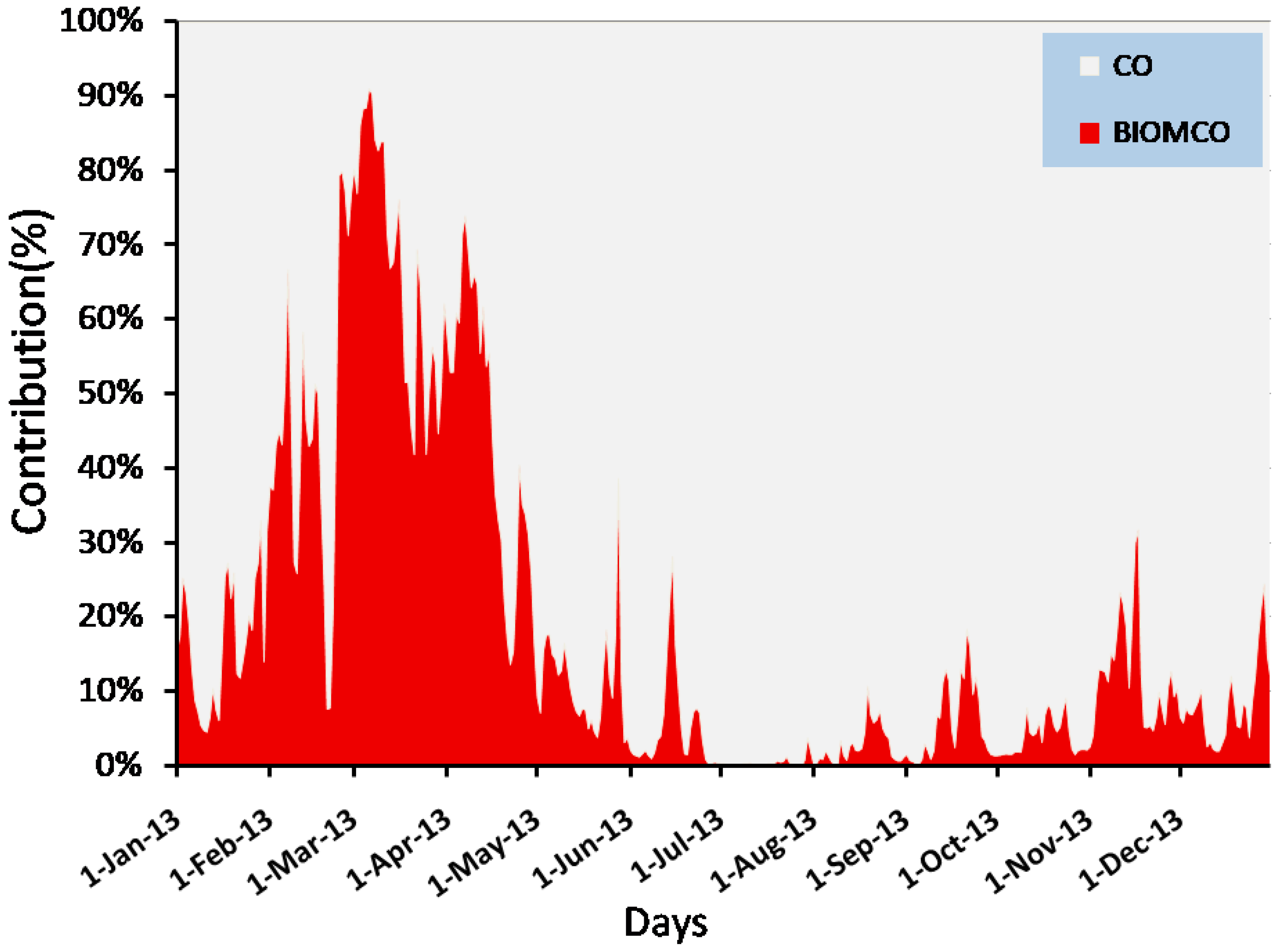
4.4. Biomass Burning/Anthropogenic Contributions

In North-Eastern India, biomass burning (BB) has been identified as one of the major sources of emission of BC and trace gases [15,34,42,101]. Kumar et al. [71] reported maximum production of CO from the BB sectors in the pre-monsoon season. During this season, in North-Eastern India, paddy fields are cleared by burning the slashes as part of jhum cultivation [89] that emits large amounts of CO and BC. The WRF-STEM model simulated BB generated CO (CO_BB) versus total CO (CO_TOT) is used to quantify the dominant sources of BC over Dibrugarh (Figure 7). The result reveals that approximately 90% of the CO is emitted from the BB sector in pre-monsoon season and 30–50 % in the late post-monsoon and winter seasons over the study location.

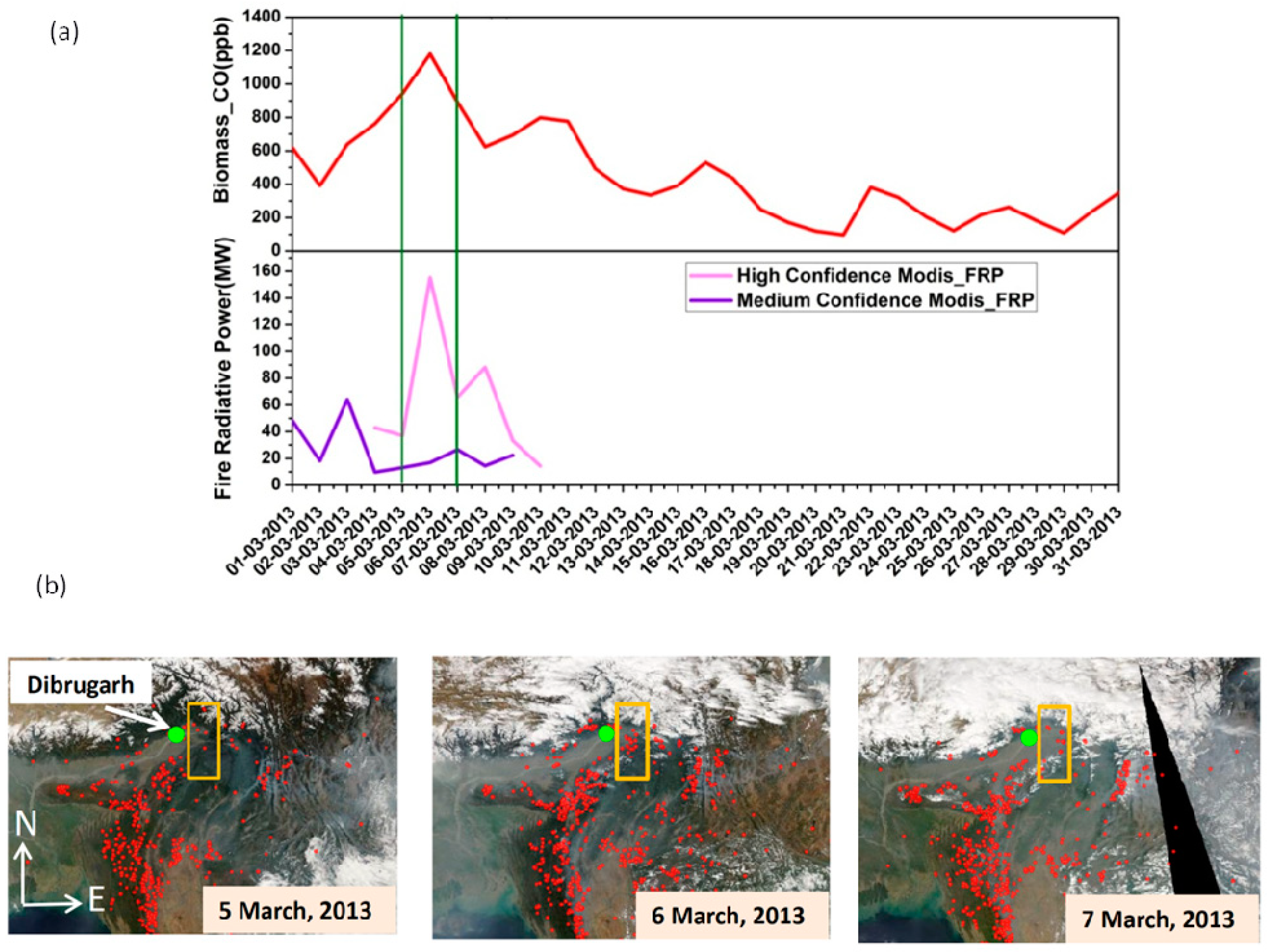
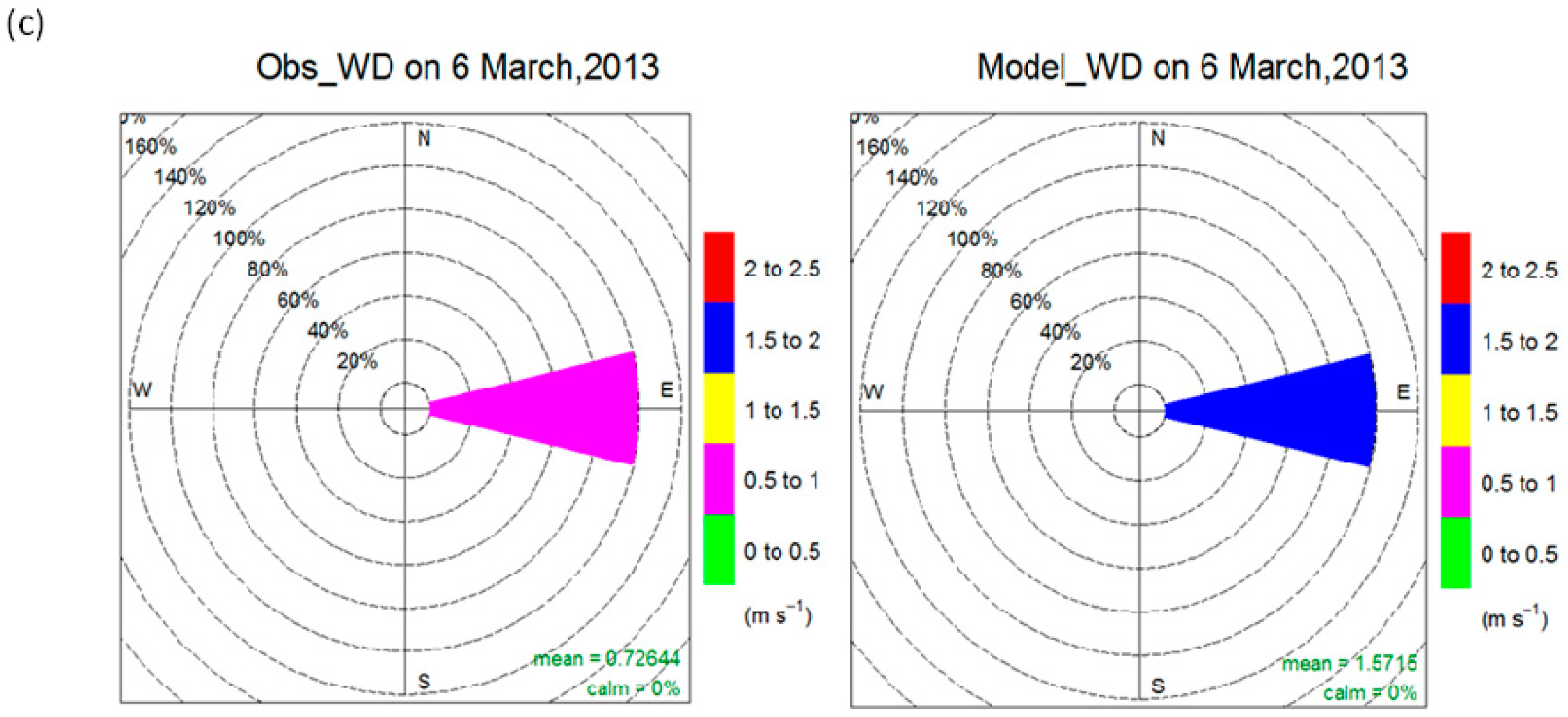
4.5. Case Study: 6 March 2013

To further investigate the cause behind the peak BB_CO level during the pre-monsoon season, we have analyzed the day-to-day variation of CO for the month of March (Figure 8a). For this, we have used the MODIS-retrieved FRP data to identify the fire events and region. The high sensitivity of the MODIS active fire product to small-scale burning within each pixel makes it potentially useful for quantifying the spatial and temporal distribution of small-scale fires in a region [34]. FRP is used to calculate the contribution of biomass burning. The FRP around the region has been divided into two categories: medium (30–80%) and high confidence (80–100%) for both Aqua and Terra FRP data products.

The high confidence FRP values estimated on 5, 6 and 7 March 2013 are 36.9, 155.25 and 65.8 MW, respectively. Because of the highest values of FRP as well as CO_BB, 6 March is considered as the event day. The medium and high confidence FRP values indicate that there are fire events taking place within 50–80 km of the monitoring site (Figure 8a), (bottom panel). The fire events are also evident from the red dots on the MODIS fire count maps (Figure 8b) on the event day (6 March) and one day before (5 March) and after (7 March) the event.

The number of fire counts enclosed by the rectangular box is more on 6 March compared to 5 and 7 March, over Dibrugarh (Figure 8b). The wind rose plot (Figure 8c) helps to understand the role of wind on the event day over the study location.

Both observed and model-simulated winds are blowing from the eastward direction towards Dibrugarh with different magnitudes (1.5–2 m/s for model and 0.5–1 m/s for observation), thereby carrying the pollutants emitted by fire (Figure 8b) activities. Moreover, BB_CO present on the rest of the days attributed to long-range transport.

4.6. Uncertainties in Model Simulations and Reanalysis Data

There exist uncertainties among models simulations and reanalysis data as mentioned in previous Section 4.1, Section 4.2 and Section 4.3.1. The differences in biases, MAE and correlation (Table 2 and Table 3, Figure 4) are due to multiple reasons. The uncertainties exist in simulating the pollutants, even when the same anthropogenic emissions data are used in the models. These may be due to each models treatment of atmospheric processes such as removal, transport, and deposition of pollutants, cloud-convection, and chemistry, etc. [81]. For example, the wet and dry deposition may affect one species but not others in the atmosphere [105]. Similarly, the dynamics i.e., the moisture content and the wind play a significant role in dispersion and dilution of the species, thereby changing the mixing ratios. In addition, the parameterizations schemes used in the models are also responsible for differences in the model simulation. In Dibrugarh, pollutants are emitted from numerous sources like automobiles and domestic stoves, oil and natural gas sectors, biomass burning, industrial sector, transportation, etc. Besides this, the concentration of pollutants varies seasonally and spatially due to as removal, transport, and deposition of pollutants, cloud-convection, and chemistry, etc. In particular, topography also plays a strong role in the temporal/spatial variation of meteorological variables, such as air temperature, precipitation [106,107] and air pollutants. Biases in models simulated terrain height will significantly affect the meteorology and air quality study. Since North-Eastern India is a complex topographic region, it is essential to do topographic correction in the models/reanalysis datasets. Similar to models, in reanalysis data, biases are associated with different numbers/types assimilation technique applied in each reanalysis. Furthermore comparison of coarser grid cell values with point measurements may also introduce errors in the calculation due to heterogeneity in elevation and land-use changes [88].

5. Conclusions

The temporal variation of meteorological variables and pollutants like CO, BC, SO₂, O_3, and NO_x over Dibrugarh located in the upper Brahmaputra basin of North-Eastern India has been investigated using surface measurements, WRF-Chem, WRF-STEM, MERRA2, and CAMS model datasets. Both model and reanalysis data captured the seasonality of meteorological variables and pollutants well but with some variability in magnitudes. The difference in magnitudes is attributed to the spatial resolution selected for the model run, underestimation of RH and overestimation of T and WS, emission inventories and model’s parameterization. The statistical quantities are computed and intercompared with surface-based measurement data to enlighten the performance of the models and reanalysis data over the study location.

The STEM tracer CO and HYSPLIT back trajectories analysis quantify the local and regional contributions of pollutants over the observation site. The transport of pollutants from various source regions and their contribution over the selected location Dibrugarh are identified North-Eastern India (59%), China (17%), IGP (14%), Bangladesh (6%), other regions of India (3%) and other regions (1% respectively). The models well captured the local/regional scale fire activities and influence of biomass burning in increasing the CO level over Dibrugarh. It is observed that 90% of the modeled simulated CO during the pre-monsoon season is due to biomass burning. The existing uncertainties in models simulation and measurements/reanalysis datasets are discussed in this study for further improvement of the datasets for future study. Overall, the air-quality models are in better agreement with observations in the pre-monsoon season especially for BC and CO. The possible reason is due to daily varying emissions from open biomass burning which is the dominant source in this period. Even the models show highest BC and CO correlation in pre-monsoon season.

References

1. Vadrevu, K.; Ohara, T.; Justice, C. Land cover, land use changes and air pollution in Asia: A synthesis. Environ. Res. Lett. 2017, 12, 120201. [Google Scholar] [CrossRef] [PubMed]
2. Gurjar, B.R.; Ravindra, K.; Nagpure, A.S. Air pollution trends over Indian megacities and their local-to-global implications. Atmos. Environ. 2016, 142, 475–495. [Google Scholar] [CrossRef]
3. Ohara, T.; Uno, I.; Wakamatsu, S.; Murano, K. Numerical simulation of the springtime trans-boundary air pollution in East Asia. Water. Air. Soil Pollut. 2001, 130, 295–300. [Google Scholar] [CrossRef]
4. Foell, W.; Green, C.; Amann, M.; Bhattacharya, S.; Carmichael, G.; Chadwick, M.; Cinderby, S.; Haugland, T.; Hettelingh, J.-P.; Hordijk, L. Energy use, emissions, and air pollution reduction strategies in Asia. Water. Air. Soil Pollut. 1995, 85, 2277–2282. [Google Scholar] [CrossRef]
5. Mallik, C.; Ghosh, D.; Ghosh, D.; Sarkar, U.; Lal, S.; Venkataramani, S. Variability of SO2, CO, and light hydrocarbons over a megacity in Eastern India: Effects of emissions and transport. Environ. Sci. Pollut. Res. 2014, 21, 8692–8706. [Google Scholar] [CrossRef]
6. Kumar, R.; Naja, M.; Satheesh, S.K.; Ojha, N.; Joshi, H.; Sarangi, T.; Pant, P.; Dumka, U.C.; Hegde, P.; Venkataramani, S. Influences of the springtime northern Indian biomass burning over the central Himalayas. J. Geophys. Res. Atmos. 2011, 116. [Google Scholar] [CrossRef]
7. Kumar, R.; Naja, M.; Pfister, G.G.; Barth, M.C.; Brasseur, G.P. Source attribution of carbon monoxide in India and surrounding regions during wintertime. J. Geophys. Res. Atmos. 2013, 118, 1981–1995. [Google Scholar] [CrossRef]
8. Lawrence, M.G.; Lelieveld, J. Atmospheric pollutant outflow from southern Asia: A review. Atmos. Chem. Phys. 2010, 10, 11017. [Google Scholar] [CrossRef]
9. Gurjar, B.R.; Ohara, T.; Khare, M.; Kulshrestha, P.; Tyagi, V.; Nagpure, A.S. South Asian Perspective: A Case of Urban Air Pollution and Potential for Climate Co-benefits in India. In Mainstreaming Climate Co-Benefits in Indian Cities; Springer: Singapore, 2018; pp. 77–98. [Google Scholar] [CrossRef]
10. Streets, D.G.; Yarber, K.F.; Woo, J.; Carmichael, G.R. Biomass burning in Asia: Annual and seasonal estimates and atmospheric emissions. Glob. Biogeochem. Cycles 2003, 17. [Google Scholar] [CrossRef]
11. Ohara, T.; Akimoto, H.; Kurokawa, J.; Horii, N.; Yamaji, K.; Yan, X.; Hayasaka, T. An Asian emission inventory of anthropogenic emission sources for the period 1980–2020. Atmos. Chem. Phys. 2007, 7, 4419–4444. [Google Scholar] [CrossRef]
12. Guttikunda, S.K.; Calori, G. A GIS based emissions inventory at 1 km × 1 km spatial resolution for air pollution analysis in Delhi, India. Atmos. Environ. 2013, 67, 101–111. [Google Scholar] [CrossRef]
13. Sheel, V.; Sahu, L.K.; Kajino, M.; Deushi, M.; Stein, O.; Nedelec, P. Seasonal and interannual variability of carbon monoxide based on MOZAIC observations, MACC reanalysis, and model simulations over an urban site in India. J. Geophys. Res. Atmos. 2014, 119, 9123–9141. [Google Scholar] [CrossRef]
14. Chandra, N.; Lal, S.; Venkataramani, S.; Patra, P.K.; Sheel, V. Temporal variations of atmospheric CO2 and CO at Ahmedabad in western India. Atmos. Chem. Phys. 2016, 16, 6153–6173. [Google Scholar] [CrossRef]
15. Bhuyan, P.K.; Bharali, C.; Pathak, B.; Kalita, G. The role of precursor gases and meteorology on temporal evolution of O3 at a tropical location in northeast India. Environ. Sci. Pollut. Res. 2014, 21, 6696–6713. [Google Scholar] [CrossRef]
16. Mallik, C.; Lal, S. Seasonal characteristics of SO2, NO2, and CO emissions in and around the Indo-Gangetic Plain. Environ. Monit. Assess. 2014, 186, 1295–1310. [Google Scholar] [CrossRef]
17. Sarangi, T.; Naja, M.; Ojha, N.; Kumar, R.; Lal, S.; Venkataramani, S.; Kumar, A.; Sagar, R.; Chandola, H.C. First simultaneous measurements of ozone, CO, and NOy at a high-altitude regional representative site in the central Himalayas. J. Geophys. Res. Atmos. 2014, 119, 1592–1611. [Google Scholar] [CrossRef]
18. Lal, S.; Sahu, L.K.; Venkataramani, S.; Mallik, C. Light non-methane hydrocarbons at two sites in the Indo-Gangetic Plain. J. Environ. Monit. 2012, 14, 1158–1165. [Google Scholar] [CrossRef]
19. Kalita, G.; Bhuyan, P.K. Spatial heterogeneity in tropospheric column ozone over the Indian subcontinent: Long-term climatology and possible association with natural and anthropogenic activities. Adv. Meteorol. 2011, 2011. [Google Scholar] [CrossRef]
20. Beig, G.; Gunthe, S.; Jadhav, D.B. Simultaneous measurements of ozone and its precursors on a diurnal scale at a semi urban site in India. J. Atmos. Chem. 2007, 57, 239–253. [Google Scholar] [CrossRef]
21. Sahu, L.K.; Lal, S. Distributions of C2–C5 NMHCs and related trace gases at a tropical urban site in India. Atmos. Environ. 2006, 40, 880–891. [Google Scholar] [CrossRef]
22. Naja, M.; Lal, S. Surface ozone and precursor gases at Gadanki (13.5 N, 79.2 E), a tropical rural site in India. J. Geophys. Res. Atmos. 2002, 107, ACH-8. [Google Scholar] [CrossRef]
23. Gaur, A.; Tripathi, S.N.; Kanawade, V.P.; Tare, V.; Shukla, S.P. Four-year measurements of trace gases (SO2, NOx, CO, and O3) at an urban location, Kanpur, in Northern India. J. Atmos. Chem. 2014, 71, 283–301. [Google Scholar] [CrossRef]
24. Carmichael, G.R.; Adhikary, B.; Kulkarni, S.; D’Allura, A.; Tang, Y.; Streets, D.; Zhang, Q.; Bond, T.C.; Ramanathan, V.; Jamroensan, A. Asian aerosols: Current and year 2030 distributions and implications to human health and regional climate change. Environ. Sci. Technol. 2009, 43, 5811–5817. [Google Scholar] [CrossRef] [PubMed]
25. Nagpure, A.S.; Gurjar, B.R.; Kumar, P. Impact of altitude on emission rates of ozone precursors from gasoline-driven light-duty commercial vehicles. Atmos. Environ. 2011, 45, 1413–1417. [Google Scholar] [CrossRef]
26. Nagpure, A.S.; Sharma, K.; Gurjar, B.R. Traffic induced emission estimates and trends (2000–2005) in megacity Delhi. Urban. Clim. 2013, 4, 61–73. [Google Scholar] [CrossRef]
27. Nagpure, A.S.; Gurjar, B.R.; Kumar, V.; Kumar, P. Estimation of exhaust and non-exhaust gaseous, particulate matter and air toxics emissions from on-road vehicles in Delhi. Atmos. Environ. 2016, 127, 118–124. [Google Scholar] [CrossRef]
28. Gurjar, B.R.; Butler, T.M.; Lawrence, M.G.; Lelieveld, J. Evaluation of emissions and air quality in megacities. Atmos. Environ. 2008, 42, 1593–1606. [Google Scholar] [CrossRef]
29. Lelieveld, J.O.; Crutzen, P.J.; Ramanathan, V.; Andreae, M.O.; Brenninkmeijer, C.A.M.; Campos, T.; Cass, G.R.; Dickerson, R.R.; Fischer, H.; De Gouw, J.A. The Indian Ocean experiment: Widespread air pollution from South and Southeast Asia. Science 2001, 291, 1031–1036. [Google Scholar] [CrossRef]
30. Nagpure, A.K.; Gurjar, B.R.; Sahni, N.; Kumar, P. Pollutant emissions from road vehicles in megacity Kolkata, India: Past and present trends. Indian J. Air Pollut. Control. 2010, 10, 18–30. [Google Scholar]
31. IPCC. Climate Change. In The Scientific Basis; Cambridge University Press: Cambridge, UK; New York, NY, USA, 2001. [Google Scholar] [CrossRef]
32. Change, C. Impacts, IPCC, Vulnerabilities and Adaptation in Developing Countries; Climate Change Secretariat: Bonn, Germany, 2007. [Google Scholar]
33. Das, D. Changing climate and its impacts on Assam, Northeast India. Bandung J. Glob. South. 2015, 2, 26. [Google Scholar] [CrossRef] [Green Version]
34. Gogoi, M.M.; Babu, S.S.; Moorthy, K.K.; Bhuyan, P.K.; Pathak, B.; Subba, T.; Chutia, L.; Kundu, S.S.; Bharali, C.; Borgohain, A. Radiative effects of absorbing aerosols over northeastern India: Observations and model simulations. J. Geophys. Res. Atmos. 2017, 122, 1132–1157. [Google Scholar] [CrossRef]
35. Central Pollution Control Board. Air Quality Monitoring, Emission Inventory and Source Apportionment Study for Indian Cities; Central Pollution Control Board: New Delhi, India, 2010. [Google Scholar]
36. Central Pollution Control Board. National Ambient Air Quality Status and Trends in India-2010; Central Pollution Control Board: New Delhi, India, 2012. [Google Scholar]
37. Bharali, C.; Pathak, B.; Bhuyan, P.K. Spring and summer night-time high ozone episodes in the upper Brahmaputra valley of North East India and their association with lightning. Atmos. Environ. 2015, 109, 234–250. [Google Scholar] [CrossRef]
38. Pathak, B.; Chutia, L.; Bharali, C.; Bhuyan, P.K. Continental export efficiencies and delineation of sources for trace gases and black carbon in North-East India: Seasonal variability. Atmos. Environ. 2016, 125, 474–485. [Google Scholar] [CrossRef]
39. Jaffe, D.; Anderson, T.; Covert, D.; Kotchenruther, R.; Trost, B.; Danielson, J.; Simpson, W.; Berntsen, T.; Karlsdottir, S.; Blake, D. Transport of Asian air pollution to North America. Geophys. Res. Lett. 1999, 26, 711–714. [Google Scholar] [CrossRef] [Green Version]
40. Seo, J.; Park, D.-S.R.; Kim, J.Y.; Youn, D.; Lim, Y.B.; Kim, Y. Effects of meteorology and emissions on urban air quality: A quantitative statistical approach to long-term records (1999–2016) in Seoul, South Korea. Atmos. Chem. Phys. 2018, 18, 16121–16137. [Google Scholar] [CrossRef] [Green Version]
41. Jain, S.K.; Kumar, V.; Saharia, M. Analysis of rainfall and temperature trends in northeast India. Int. J. Climatol. 2013, 33, 968–978. [Google Scholar] [CrossRef]
42. Pathak, B.; Kalita, G.; Bhuyan, K.; Bhuyan, P.K.; Moorthy, K.K. Aerosol temporal characteristics and its impact on shortwave radiative forcing at a location in the northeast of India. J. Geophys. Res. Atmos. 2010, 115. [Google Scholar] [CrossRef] [Green Version]
43. Hansen, A.D.A.; Rosen, H.; Novakov, T. The aethalometer—An instrument for the real-time measurement of optical absorption by aerosol particles. Sci. Total Environ. 1984, 36, 191–196. [Google Scholar] [CrossRef] [Green Version]
44. Arnott, W.P.; Hamasha, K.; Moosmüller, H.; Sheridan, P.J.; Ogren, J.A. Towards aerosol light-absorption measurements with a 7-wavelength aethalometer: Evaluation with a photoacoustic instrument and 3-wavelength nephelometer. Aerosol Sci. Technol. 2005, 39, 17–29. [Google Scholar] [CrossRef]
45. Weingartner, E.; Saathoff, H.; Schnaiter, M.; Streit, N.; Bitnar, B.; Baltensperger, U. Absorption of light by soot particles: Determination of the absorption coefficient by means of aethalometers. J. Aerosol Sci. 2003, 34, 1445–1463. [Google Scholar] [CrossRef]
46. Giglio, L.; Schroeder, W.; Justice, C.O. The collection 6 MODIS active fire detection algorithm and fire products. Remote Sens. Environ. 2016, 178, 31–41. [Google Scholar] [CrossRef] [PubMed] [Green Version]
47. Subba, T.; Gogoi, M.M.; Pathak, B.; Ajay, P.; Bhuyan, P.K.; Solmon, F. Assessment of 1D and 3D model simulated radiation flux based on surface measurements and estimation of aerosol forcing and their climatological aspects. Atmos. Res. 2018, 204, 110–127. [Google Scholar] [CrossRef]
48. Grell, G.A.; Peckham, S.E.; Schmitz, R.; McKeen, S.A.; Frost, G.; Skamarock, W.C.; Eder, B. Fully coupled “online” chemistry within the WRF model. Atmos. Environ. 2005, 39, 6957–6975. [Google Scholar] [CrossRef]
49. Skamarock, W.C.; Klemp, J.B.; Dudhia, J.; Gill, D.O.; Barker, D.M.; Wang, W.; Powers, J.G. A Description of the Advanced Research WRF Version 3; University Corporation for Atmospheric Research: Boulder, CO, USA, 2008; Available online: https://opensky.ucar.edu/islandora/object/technotes:500 (accessed on 20 January 2019). [CrossRef]
50. Wiedinmyer, C.; Akagi, S.K.; Yokelson, R.J.; Emmons, L.K.; Al-Saadi, J.A.; Orlando, J.J.; Soja, A.J. The Fire INventory from NCAR (FINN): A high resolution global model to estimate the emissions from open burning. Geosci. Model. Dev. 2011, 4, 625. [Google Scholar] [CrossRef] [Green Version]
51. Thompson, G.; Field, P.R.; Rasmussen, R.M.; Hall, W.D. Explicit Forecasts of Winter Precipitation Using an Improved Bulk Microphysics Scheme. Part II: Implementation of a New Snow Parameterization. Mon. Weather Rev. 2008, 136, 5095–5115. [Google Scholar] [CrossRef]
52. Kain, J.S. The Kain–Fritsch Convective Parameterization: An Update. J. Appl. Meteorol. 2004, 43, 170–181. [Google Scholar] [CrossRef] [Green Version]
53. Hong, S.-Y.; Noh, Y.; Dudhia, J. A New Vertical Diffusion Package with an Explicit Treatment of Entrainment Processes. Mon. Weather Rev. 2006, 134, 2318–2341. [Google Scholar] [CrossRef] [Green Version]
54. Dudhia, J. Numerical study of convection observed during the winter monsoon experiment using a mesoscale two-dimensional model. J. Atmos. Sci. 1989, 46, 3077–3107. [Google Scholar] [CrossRef]
55. Mlawer, E.J.; Taubman, S.J.; Brown, P.D.; Iacono, M.J.; Clough, S.A. Radiative transfer for inhomogeneous atmospheres: RRTM, a validated correlated-k model for the longwave. J. Geophys. Res. Atmos. 1997, 102, 16663–16682. [Google Scholar] [CrossRef] [Green Version]
56. Madronich, S.; Weller, G. Numerical integration errors in calculated tropospheric photodissociation rate coefficients. J. Atmos. Chem. 1990, 10, 289–300. [Google Scholar] [CrossRef]
57. Adhikary, B.; Carmichael, G.R.; Kulkarni, S.; Wei, C.; Tang, Y.; D’Allura, A.; Mena-Carrasco, M.; Streets, D.G.; Zhang, Q.; Pierce, R.B. A Regional Scale Modeling Analysis of Aerosol and Trace Gas. Distributions over the Eastern Pacific during the INTEX-B Field Campaign. Atmos. Chem. Phys. 2010, 10, 2091–2115. [Google Scholar] [CrossRef] [Green Version]
58. Kulkarni, S.; Sobhani, N.; Miller-Schulze, J.P.; Shafer, M.M.; Schauer, J.J.; Solomon, P.A.; Saide, P.E.; Spak, S.N.; Cheng, Y.F.; Denier Van Der Gon, H.A.C. Source sector and region contributions to BC and PM 2.5 in Central Asia. Atmos. Chem. Phys. 2015, 15, 1683–1705. [Google Scholar] [CrossRef] [Green Version]
59. Wei, C. Modeling the Effects of Heterogeneous Reactions on Atmospheric Chemistry and Aerosol Properties. Available online: https://www.semanticscholar.org/paper/Modeling-the-effects-of-heterogeneous-reactions-on-Wei/56ecffca3a531d3463470e0b1e02c8da59838039 (accessed on 25 December 2018).
60. Janssens-Maenhout, G.; Crippa, M.; Guizzardi, D.; Dentener, F.; Muntean, M.; Pouliot, G.; Keating, T.; Zhang, Q.; Kurokawa, J.; Wankmüller, R. HTAP_v2: A mosaic of regional and global emission gridmaps for 2008 and 2010 to study hemispheric transport of air pollution. Atmos. Chem. Phys. Discuss. 2015, 15, 11411–11432. [Google Scholar] [CrossRef] [Green Version]
61. Wiedinmyer, C.; Quayle, B.; Geron, C.; Belote, A.; McKenzie, D.; Zhang, X.; O’Neill, S.; Wynne, K.K. Estimating emissions from fires in North America for air quality modeling. Atmos. Environ. 2006, 40, 3419–3432. [Google Scholar] [CrossRef]
62. Draxler, R.R.; Hess, G.D. An overview of the HYSPLIT_4 modelling system for trajectories. Aust. Meteorol. Mag. 1998, 47, 295–308. [Google Scholar]
63. Ward, J.H., Jr. Hierarchical grouping to optimize an objective function. J. Am. Stat. Assoc. 1963, 58, 236–244. [Google Scholar] [CrossRef]
64. Cheng, S.; Wang, F.; Li, J.; Chen, D.; Li, M.; Zhou, Y.; Ren, Z. Application of trajectory clustering and source apportionment methods for investigating trans-boundary atmospheric PM10 pollution. Aerosol Air Qual. Res. 2013, 13, 333–342. [Google Scholar] [CrossRef]
65. Flemming, J.; Benedetti, A.; Inness, A.; Engelen, R.J.; Jones, L.; Huijnen, V.; Remy, S.; Parrington, M.; Suttie, M.; Bozzo, A.; et al. The CAMS interim Reanalysis of Carbon Monoxide, Ozone and Aerosol for 2003–2015. Atmos. Chem. Phys. 2017, 17, 1945–1983. [Google Scholar] [CrossRef] [Green Version]
66. MERRA-2: Initial Evaluation of the Climate. Available online: https://gmao.gsfc.nasa.gov/pubs/docs/Bosilovich803.pdf (accessed on 10 August,2019).
67. Rienecker, M.M.; Suarez, M.J.; Gelaro, R.; Todling, R.; Bacmeister, J.; Liu, E.; Bosilovich, M.G.; Schubert, S.D.; Takacs, L.; Kim, G.-K.; et al. MERRA: NASA’s Modern-Era Retrospective Analysis for Research and Applications. J. Clim. 2011, 24, 3624–3648. [Google Scholar] [CrossRef]
68. Chin, M.; Ginoux, P.; Kinne, S.; Torres, O.; Holben, B.N.; Duncan, B.N.; Martin, R.V.; Logan, J.A.; Higurashi, A.; Nakajima, T. Tropospheric aerosol optical thickness from the GOCART model and comparisons with satellite and Sun photometer measurements. J. Atmos. Sci. 2002, 59, 461–483. [Google Scholar] [CrossRef]
69. Colarco, P.; da Silva, A.; Chin, M.; Diehl, T. Online simulations of global aerosol distributions in the NASA GEOS-4 model and comparisons to satellite and ground-based aerosol optical depth. J. Geophys. Res. 2010, 115, D14207. [Google Scholar] [CrossRef] [Green Version]
70. Wargan, K.; Labow, G.; Frith, S.; Pawson, S.; Livesey, N.; Partyka, G. Evaluation of the Ozone Fields in NASA’s MERRA-2 Reanalysis. J. Clim. 2017, 30, 2961–2988. [Google Scholar] [CrossRef] [PubMed] [Green Version]
71. Kumar, R.; Naja, M.; Pfister, G.G.; Barth, M.C.; Wiedinmyer, C.; Brasseur, G.P. Simulations over South Asia using the Weather Research and Forecasting model with Chemistry (WRF-Chem): Chemistry evaluation and initial results. Geosci. Model. Dev. 2012, 5, 619–648. [Google Scholar] [CrossRef] [Green Version]
72. Kumar, R.; Barth, M.C.; Nair, V.S.; Pfister, G.G.; Suresh Babu, S.; Satheesh, S.K.; Krishna Moorthy, K.; Carmichael, G.R.; Lu, Z.; Streets, D.G. Sources of black carbon aerosols in South Asia and surrounding regions during the Integrated Campaign for Aerosols, Gases and Radiation Budget (ICARB). Atmos. Chem. Phys. 2015, 15, 5415–5428. [Google Scholar] [CrossRef] [Green Version]
73. Bharali, C.; Nair, V.S.; Chutia, L.; Babu, S.S. Modeling of the Effects of Wintertime Aerosols on Boundary Layer Properties Over the Indo Gangetic Plain. J. Geophys. Res. Atmos. 2019, 124, 4141–4157. [Google Scholar] [CrossRef]
74. Sharma, A.; Ojha, N.; Pozzer, A.; Mar, K.A.; Beig, G.; Lelieveld, J.; Gunthe, S.S. WRF-Chem simulated surface ozone over south Asia during the pre-monsoon: Effects of emission inventories and chemical mechanisms. Atmos. Chem. Phys. 2017, 17, 14393–14413. [Google Scholar] [CrossRef] [Green Version]
75. Gul, C.; Puppala, S.P.; Kang, S.; Adhikary, B.; Zhang, Y.; Ali, S.; Li, Y.; Li, X. Concentrations and source regions of light-absorbing particles in snow/ice in northern Pakistan and their impact on snow albedo. Atmos. Chem. Phys. 2018, 18, 4981–5000. [Google Scholar] [CrossRef] [Green Version]
76. Rupakheti, D.; Adhikary, B.; Praveen, P.S.; Rupakheti, M.; Kang, S.; Mahata, K.S.; Naja, M.; Zhang, Q.; Panday, A.K.; Lawrence, M.G. Pre-monsoon air quality over Lumbini, a world heritage site along the Himalayan foothills. Atmos. Chem. Phys. 2017, 17, 11041. [Google Scholar] [CrossRef] [Green Version]
77. Pathak, B.; Borgohain, A.; Bhuyan, P.K.; Kundu, S.S.; Sudhakar, S.; Gogoi, M.M.; Takemura, T. Spatial heterogeneity in near surface aerosol characteristics across the Brahmaputra valley. J. Earth Syst. Sci. 2014, 123, 651–663. [Google Scholar] [CrossRef]
78. Brunner, D.; Savage, N.; Jorba, O.; Eder, B.; Giordano, L.; Badia, A.; Balzarini, A.; Baro, R.; Bianconi, R.; Chemel, C. Comparative analysis of meteorological performance of coupled chemistry-meteorology models in the context of AQMEII phase 2. Atmos. Environ. 2015, 115, 470–498. [Google Scholar] [CrossRef]
79. Eccel, E. Estimating air humidity from temperature and precipitation measures for modelling applications. Meteorol. Appl. 2012, 19, 118–128. [Google Scholar] [CrossRef]
80. Ali, H.; Mishra, V. Contrasting response of rainfall extremes to increase in surface air and dewpoint temperatures at urban locations in India. Sci. Rep. 2017, 7, 1228. [Google Scholar] [CrossRef] [PubMed] [Green Version]
81. Pan, X.; Chin, M.; Gautam, R.; Bian, H.; Kim, D.; Colarco, P.R.; Diehl, T.L.; Takemura, T.; Pozzoli, L.; Tsigaridis, K. A multi-model evaluation of aerosols over South Asia: Common problems and possible causes. Atmos. Chem. Phys. 2015, 15, 5903–5928. [Google Scholar] [CrossRef] [Green Version]
82. Chawla, A.; Spindler, D.M.; Tolman, H.L. Validation of a thirty year wave hindcast using the Climate Forecast System Reanalysis winds. Ocean. Model. 2013, 70, 189–206. [Google Scholar] [CrossRef]
83. Seidel, D.J.; Ao, C.O.; Li, K. Estimating climatological planetary boundary layer heights from radiosonde observations: Comparison of methods and uncertainty analysis. J. Geophys. Res. Atmos. 2010, 115. [Google Scholar] [CrossRef] [Green Version]
84. Si, Y.; Li, S.; Chen, L.; Yu, C.; Wang, Z.; Wang, Y.; Wang, H. Validation and Spatiotemporal Distribution of GEOS-5–Based Planetary Boundary Layer Height and Relative Humidity in China. Adv. Atmos. Sci. 2018, 35, 479–492. [Google Scholar] [CrossRef]
85. Chai, T.; Draxler, R.R. Root mean square error (RMSE) or mean absolute error (MAE)?—Arguments against avoiding RMSE in the literature. Geosci. Model. Dev. 2014, 7, 1247–1250. [Google Scholar] [CrossRef] [Green Version]
86. Sayegh, A.S.; Munir, S.; Habeebullah, T.M. Comparing the performance of statistical models for predicting PM10 concentrations. Aerosol Air Qual. Res. 2014, 14, 653–665. [Google Scholar] [CrossRef] [Green Version]
87. Mues, A.; Lauer, A.; Lupascu, A.; Rupakheti, M.; Kuik, F.; Lawrence, M.G. WRF and WRF-Chem v3. 5.1 simulations of meteorology and black carbon concentrations in the Kathmandu Valley. Geosci. Model. Dev. 2018, 11, 2067–2091. [Google Scholar] [CrossRef] [Green Version]
88. Wang, A.; Zeng, X. Evaluation of multireanalysis products with in situ observations over the Tibetan Plateau. J. Geophys. Res. Atmos. 2012, 117. [Google Scholar] [CrossRef]
89. Pathak, B.; Bhuyan, P.K.; Biswas, J.; Takemura, T. Long term climatology of particulate matter and associated microphysical and optical properties over Dibrugarh, North-East India and inter-comparison with SPRINTARS simulations. Atmos. Environ. 2013, 69, 334–344. [Google Scholar] [CrossRef]
90. Puliafito, S.E.; Allende, D.G.; Castesana, P.S.; Ruggeri, M.F. High-resolution atmospheric emission inventory of the argentine energy sector. Comparison with Edgar global emission database. Heliyon 2017, 3, e00489. [Google Scholar] [CrossRef] [Green Version]
91. Ganguly, D.; Rasch, P.J.; Wang, H.; Yoon, J.-H. Climate response of the South Asian monsoon system to anthropogenic aerosols. J. Geophys. Res. Atmos. 2012, 117. [Google Scholar] [CrossRef] [Green Version]
92. Menon, S.; Koch, D.; Beig, G.; Sahu, S.; Fasullo, J.; Orlikowski, D. Black carbon aerosols and the third polar ice cap. Atmos. Chem. Phys. 2010, 10, 4559–4571. [Google Scholar] [CrossRef] [Green Version]
93. Nair, V.S.; Solmon, F.; Giorgi, F.; Mariotti, L.; Babu, S.S.; Moorthy, K.K. Simulation of South Asian aerosols for regional climate studies. J. Geophys. Res. Atmos. 2012, 117. [Google Scholar] [CrossRef]
94. Moorthy, K.K.; Beegum, S.N.; Srivastava, N.; Satheesh, S.K.; Chin, M.; Blond, N.; Babu, S.S.; Singh, S. Performance evaluation of chemistry transport models over India. Atmos. Environ. 2013, 71, 210–225. [Google Scholar] [CrossRef]
95. Kumar, R.; Barth, M.C.; Pfister, G.G.; Nair, V.S.; Ghude, S.D.; Ojha, N. What controls the seasonal cycle of black carbon aerosols in India? J. Geophys. Res. Atmos. 2015, 120, 7788–7812. [Google Scholar] [CrossRef] [Green Version]
96. Govardhan, G.; Nanjundiah, R.S.; Satheesh, S.K.; Krishnamoorthy, K.; Kotamarthi, V.R. Performance of WRF-Chem over Indian region: Comparison with measurements. J. Earth Syst. Sci. 2015, 124, 875–896. [Google Scholar] [CrossRef] [Green Version]
97. Zhang, H.; Wang, Y.; Hu, J.; Ying, Q.; Hu, X.-M. Relationships between meteorological parameters and criteria air pollutants in three megacities in China. Environ. Res. 2015, 140, 242–254. [Google Scholar] [CrossRef]
98. Granier, C.; Bessagnet, B.; Bond, T.; D’Angiola, A.; Denier van der Gon, H.; Frost, G.J.; Heil, A.; Kaiser, J.W.; Kinne, S.; Klimont, Z.; et al. Evolution of anthropogenic and biomass burning emissions of air pollutants at global and regional scales during the 1980–2010 period. Clim. Chang. 2011, 109, 163–190. [Google Scholar] [CrossRef]
99. Amnuaylojaroen, T.; Barth, M.C.; Emmons, L.K.; Carmichael, G.R.; Kreasuwun, J.; Prasitwattanaseree, S.; Chantara, S. Effect of different emission inventories on modeled ozone and carbon monoxide in Southeast Asia. Atmos. Chem. Phys. 2014, 14, 12983–13012. [Google Scholar] [CrossRef] [Green Version]
100. Ma, J.; Van Aardenne, J.A. Impact of different emission inventories on simulated tropospheric ozone over China: A regional chemical transport model evaluation. Atmos. Chem. Phys. 2004, 4, 877–887. [Google Scholar] [CrossRef] [Green Version]
101. Zhong, M.; Saikawa, E.; Liu, Y.; Naik, V.; Horowitz, L.W.; Takigawa, M.; Zhao, Y.; Lin, N.-H.; Stone, E.A. Air quality modeling with WRF-Chem v3.5 in East Asia: Sensitivity to emissions and evaluation of simulated air quality. Geosci. Model Dev. 2016, 9, 1201–1218. [Google Scholar] [CrossRef] [Green Version]
102. Seinfeld, J.H.; Pandis, S.N.; Noone, K. Atmospheric chemistry and physics: From air pollution to climate change. Phys. Today 1998, 51, 88. [Google Scholar] [CrossRef]
103. Chen, D.; Wang, Y.; McElroy, M.B.; He, K.; Yantosca, R.M.; Sager, P. Le Regional CO pollution and export in China simulated by the high-resolution nested-grid GEOS-Chem model. Atmos. Chem. Phys. 2009, 9, 3825–3839. [Google Scholar] [CrossRef] [Green Version]
104. Price, H.U.; Jaffe, D.A.; Doskey, P.V.; McKendry, I.; Anderson, T.L. Vertical profiles of O3, aerosols, CO and NMHCs in the northeast Pacific during the TRACE-P and ACE-Asia experiments. J. Geophys. Res. Atmos. 2003, 108. [Google Scholar] [CrossRef]
105. Wang, Y.; Wang, X.; Kondo, Y.; Kajino, M.; Munger, J.W.; Hao, J. Black carbon and its correlation with trace gases at a rural site in Beijing: Top-down constraints from ambient measurements on bottom-up emissions. J. Geophys. Res. Atmos. 2011, 116. [Google Scholar] [CrossRef]
106. Berg, A.A.; Famiglietti, J.S.; Walker, J.P.; Houser, P.R. Impact of bias correction to reanalysis products on simulations of North American soil moisture and hydrological fluxes. J. Geophys. Res. Atmos. 2003, 108. [Google Scholar] [CrossRef] [Green Version]
107. Zhao, T.; Guo, W.; Fu, C. Calibrating and evaluating reanalysis surface temperature error by topographic correction. J. Clim. 2008, 21, 1440–1446. [Google Scholar] [CrossRef]
Figure 1. (a) The white box highlights the North-Eastern India region, the star indicates the study location of Dibrugarh (b) North-Eastern India map showing the emission sources (the background of the map is taken from www.naturalearthdata.com).
Atmosphere 10 00703 g001aAtmosphere 10 00703 g001b
Figure 2. variation of daily averaged atmospheric pressure (P); temperature (T); relative humidity (RH); wind speed (WS); wind direction (WD); planetary boundary layer height (PBLH) are presented using observation (red), WRF-Chem (blue), STEM (green), CAMS (yellow) and MERRA2 (magenta) over Dibrugarh from December 2012 to November 2013. (WRF-Chem: Weather Research and Forecasting model coupled with chemistry, STEM: Sulfur Transport dEposition Model, CAMS: Copernicus Atmosphere Monitoring Service, MERRA2: Modern-Era Retrospective Analysis for Research and Applications, Version 2).
Atmosphere 10 00703 g002
Figure 3. Variation of the surface measured, model-simulated and reanalysis BC, CO, SO2, O3 and NOx over Dibrugarh for the year 2013.
Atmosphere 10 00703 g003
Figure 4. BC–CO correlation plots from surface observation, WRF-Chem, WRF-STEM, CAMS and MERRA2 over Dibrugarh are presented (a) Winter, (b) Pre-monsoon, (c) Monsoon and (d) Post-Monsoon.
Atmosphere 10 00703 g004aAtmosphere 10 00703 g004b
Figure 5. (a) Time series of regional contributions of anthropogenic CO over Dibrugarh (b) Annual anthropogenic CO contribution from different regions.
Atmosphere 10 00703 g005aAtmosphere 10 00703 g005b
Figure 6. Seasonal clusters of daily 5-day back trajectories from Dec 2012 to Nov 2013 arriving at 500 m AGL over Dibrugarh.
Atmosphere 10 00703 g006
Figure 7. Temporal distribution of biomass burning CO (BIOMCO) over Dibrugarh.
Atmosphere 10 00703 g007
Figure 8. (a) Model-simulated biomass burning generated CO during the month of March 2013, and MODIS-retrieved FRP for the same period; (b) Fire count map showing the fire events on 5, 6 and 7 March 2013. (c) A wind rose plots to shows the wind profile on the event days.
Atmosphere 10 00703 g008aAtmosphere 10 00703 g008b