Estimation of Low-Flow in South Korean River Basins Using a Canonical Correlation Analysis and Neural Network (CCA-NN) Based Regional Frequency Analysis

Abstract

Low-flow quantiles at ungauged locations are generally estimated based on hydrological methods, such as the drainage area ratio and frequency analysis methods. In practice, the drainage area ratio approach is a popular but simple linear model. When hydrologically nonlinear characteristics govern the runoff process, the linear approach leads to significant bias. This study was conducted to develop an improved nonlinear approach using a canonical correlation analysis and neural network (CCA-NN)-based regional frequency analysis (RFA) for low-flow estimation. The jackknife technique was utilized to validate the two methods. The approaches were applied to 33 river basins in South Korea. In this work, we focused on two-year and five-year return periods. For the two-year return period, the BIAS, RMSE, and R² were 0.013, 0.511, and 0.408 with the RFA, respectively, and −0.042, 1.042, and 0.114 with the drainage area ratio method, respectively; whereas for the five-year return period, the respective indices were −0.018, 0.316, and 0.573 with RFA, respectively, and 0.166, 0.536, and 0.044 with the drainage area ratio method, respectively. RFA outperformed the drainage area ratio method based on its high prediction accuracy and ability to avoid the bias problem. This study indicates that machine learning-based nonlinear techniques have the potential for use in estimating reliable low-flows at ungauged sites.

1. Introduction

Reliable low-flow estimates are necessary to provide information for water supply planning, reservoir storage design, water quantity and quality preservation, irrigation, hydropower production, and pollution load dispersion [1,2,3,4]. In the case of insufficient or no streamflow records, several approaches can be used to obtain low-flow estimates. For example, regression models, including linear methods, can be applied with explanatory variables that are determined by physiographical and meteorological characteristics. Additionally, several studies with nonlinear models have been conducted to provide more reliable low-flow estimates [5,6,7].

The drainage area ratio method is a linear model between the drainage area and discharge and has been popular for the estimation of low-flow with a 10/365 non-exceedance probability [8]. A number of studies have applied the drainage area ratio method. Wiche et al. [9] examined historic streamflow data by focusing on the James River in North Dakota and South Dakota, USA and performed record extension based on different techniques, such as the drainage area ratio method. Guenthner et al. [10] and Emerson and Dressler [11] studied monthly gauged and estimated streamflow for the Red River, USA and used the drainage area ratio approach to develop streamflow records. Cho et al. [12] investigated low-flows during a dry season in South Korea to obtain low-flow estimates at ungauged sites based on three approaches, including the drainage area ratio method.

The regional frequency analysis (RFA) method has been widely used to assess hydrological characteristics at locations with little or no data available. The hydrological estimations that are derived from RFA are of prime significance in the design of hydraulic structures such as dams and reservoirs. In RFA, two principal steps are required: (a) the identification of groups of basins (homogenous regions) that are hydrologically similar to a target basin and (b) model application for regional estimation within the homogenous regions. These regions have been traditionally defined using geographical and administrative boundaries considering hydrological features [13,14]. The region of influence approach, which pools a certain number of river basins based on proximity in a catchment feature space, has also been utilized to define homogenous regions with objective functions [15,16,17]. In recent studies, the canonical correlation analysis (CCA) was recommended and used to determine hydrologically similar regions by creating a canonical space and providing the optimal number of stations in the regions [18].

As a common nonlinear regression approach, artificial neural networks (ANNs) have been broadly adopted for a wide range of hydrological problems. Luk et al. [19] performed rainfall forecasting using an ANN over an urban catchment in Australia. Shu and Burn [20] and Dawson et al. [21] used an ANN for indexing floods and flood quantile estimation based on catchments in the United Kingdom (UK) by improving a hydrological prediction model. Seidou et al. [22] also applied an ANN for the regional estimation of lake ice thickness at ungauged locations in Canada. Shu and Ouarda [23] used regional frequency analysis based on ANN models to obtain flood quantile estimations for 151 river networks in the province of Quebec, Canada. Ouarda and Shu [3] conducted a regional low-flow frequency analysis using an ANN model with low-flow quantiles of the summer and winter seasons based on selected river basins in Canada.

The main objectives of the present study are to develop an advanced method of obtaining low-flow estimates in ungauged basins and to identify the relationships between physiographical/meteorological variables and hydrological variables in South Korea. A regional low-flow estimation approach based on CCA and ANNs for RFA is proposed and compared with the drainage area ratio method. CCA is used to identify the canonical space that is the transformed space to obtain continuous hydrologic variables. In this space, the prediction performance of the original data is preserved and redundant information is excluded to improve the estimates. CCA also identifies projections of high correlations between the two sets of multivariate variables by providing canonical variables that are linear combinations of the variables. ANNs are then used to establish the nonlinear relationships between the canonical variables and hydrological variables to be estimated. We will provide more details about these processes in the methodology section.

The remainder of the paper is organized as follows. In Section 2, the data set that was used in the present study is described. Section 3 presents the methodologies that were used in the analysis to obtain low-flow estimates with assessments based on the proposed models. The results and discussion are given in Section 4. Finally, conclusions are summarized in Section 5.

2. Data Set

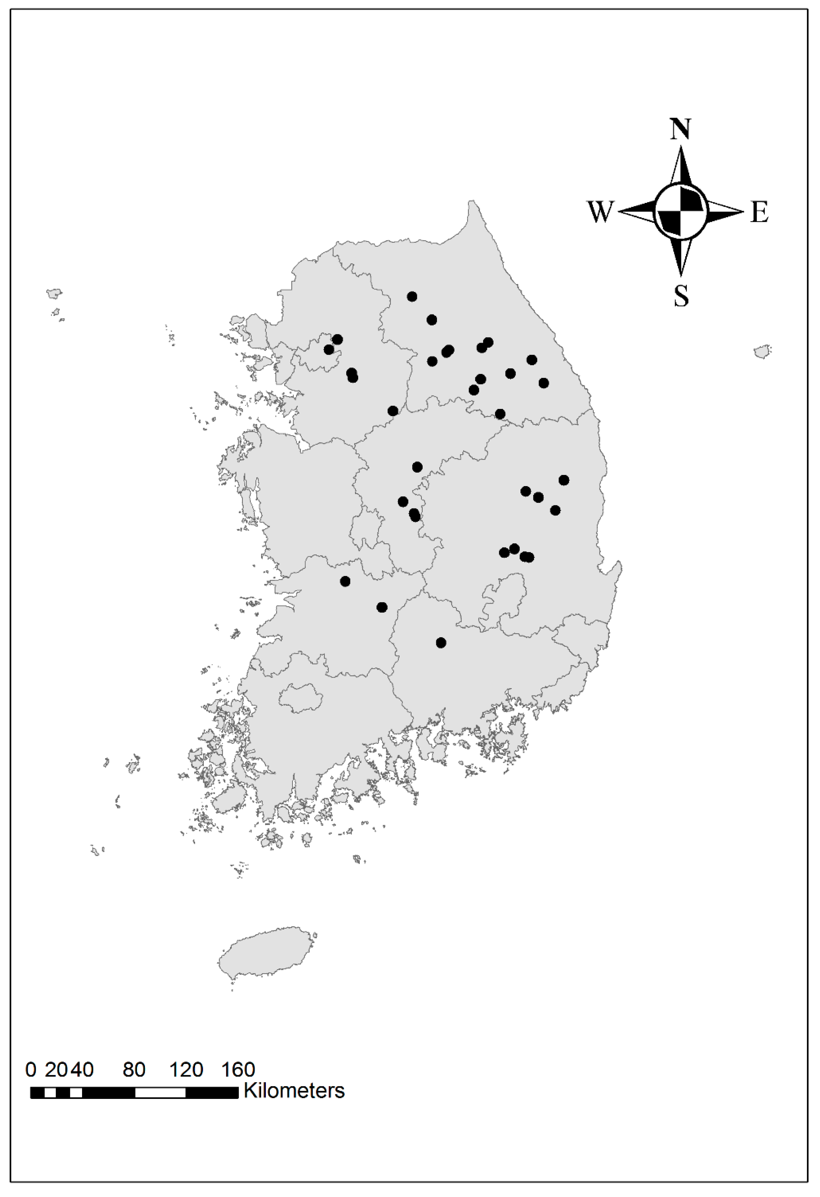
A data set of 33 river basins in South Korea was created to estimate the low-flow values in ungauged basins. The variables of the river basins that were used for this study are shown in

Table 1. Variables for the 33 river basins that were used in the study.

River	Basin Area (km2)	Mean Basin Slope (m/m)	Main Channel Length (km)	Main Channel Slope (m/m)	Curve Number (-)	Annual Mean Precipitation (mm)	Annual Mean Temperature (Degree)
Imokjeonggyo	58	0.387	17.408	0.057	78.6	1493.75	8.69
Baekokpogyo	108	0.365	26.96	0.039	78.525	1474.99	8.79
Youngyang	316	0.388	37.815	0.027	78.325	1082.01	11.56
Cheongsong	309	0.367	43.338	0.018	78.863	1014.27	11.78
Donggok	80	0.412	15.89	0.044	78.924	1024.87	11.94
Goro	109	0.395	20.873	0.034	78.879	1028.86	12.04
Epyunggyo	49	0.342	16.582	0.028	78.228	1284.02	11.25
Tanbugyo	81	0.358	24.026	0.038	78.157	1269.26	11.66
Gidaegyo	355	0.286	38.48	0.026	78.317	1280.81	11.46
Soyanggang Dam	2768	0.418	150.949	0.01	79.308	1373.38	9.93
Goesan Dam	682	0.338	84.788	0.011	77.78	1252.27	11.51
Andong Dam	1600	0.378	154.767	0.009	78.912	1179.04	10.47
Imha Dam	1375	0.355	91.697	0.012	78.885	1017.32	11.37
Hapcheon Dam	927	0.329	70.821	0.02	79.11	1319.49	12.12
Wonju	116	0.402	24.75	0.032	77.753	1278.73	10.65
Dopyeong	150	0.288	26.043	0.024	78.458	1409.99	11.15
Imgye	162	0.346	18.621	0.046	78.018	1446.55	9.95
Maeil	180	0.374	28.295	0.038	78.316	1320.69	10.71
Toegyewon	206	0.267	32.625	0.024	78.865	1465.12	11.71
Jungnanggyo	217	0.207	33.372	0.023	79.863	1465.34	11.88
Gyeongan	290	0.236	38.118	0.015	78.582	1411.57	11.11
Heukcheongyo	167	0.379	25.676	0.042	78.365	1441.25	9.71
Hoengseong	453	0.361	52.886	0.022	78.422	1422.68	10.21
Hwachon	535	0.383	60.294	0.017	78.966	1405.84	9.73
Chungmi	512	0.18	53.531	0.012	77.29	1300.61	11.54
Pyeong Chang	757	0.387	82.742	0.016	78.521	1429.93	9.71
Misung	172	0.344	34.758	0.022	78.592	1045.42	11.92
Hyoryeong	150	0.32	23.927	0.046	78.606	1051.36	12.05
Cheoncheon	287	0.312	32.715	0.037	79.055	1379.14	11.26
Gosan	288	0.396	27.401	0.038	78.379	1312.09	12.45
Cheongseon2	1460	0.409	93.27	0.013	78.02	1386.34	10.05
Yeongwol	494	0.464	54.113	0.026	78.582	1237.08	10.06
Banglimgyo	826	0.387	106.807	0.013	78.518	1366.94	9.69

. Figure 1 shows the outlet of each basin selected in the present study based on the following criteria.

• A historical flow record of 10 years or longer is available for the analysis.
• The gauged catchment has a flow regime with minimal human intervention.
• The historical data pass the stationarity [24] and independence [25] tests.

To conduct RFA, several variables representing the physiographical and meteorological features were obtained for the river networks in South Korea. In this study, we set seven variables that have generally been used in previous studies with RFA [3,18,23,26]. These variables include the drainage area (AREA), mean basin slope (MBS), annual mean precipitation (AMP), annual mean temperature (AMT), length of the main channel (MCL), slope of the main channel (MCS), and curve number (CN). A brief description with statistics for all the variables that were used in the analysis is given in

Table 2. Descriptive statistics of the hydrological, physiographical, and meteorological variables for the 33 watersheds that were used in this study.

Variable	Unit	Mean	Max	Min	Standard Deviation	Skewness	Kurtosis
Basin area	km2	492.106	2768.273	49.183	578.452	2.427	6.858
Mean basin slope	m/m	0.350	0.464	0.180	0.062	−1.087	1.265
Main channel length	km	49.828	154.767	15.890	36.351	1.607	2.186
Main channel slope	m/m	0.027	0.057	0.009	0.013	0.474	−0.677
Curve number	−	78.545	79.863	77.290	0.488	0.006	1.382
Annual mean precipitation	mm	1293.061	1493.752	1014.268	154.377	−0.703	−0.774
Annual mean temperature	degree	10.913	12.455	8.694	1.011	−0.547	−0.707

.

For the hydrological variables that are related to low-flows in the present work, the specific quantiles, such as the two-year and five-year quantiles, are calculated based on the flow records from all the gauged sites in the study area. Cho et al. [12] investigated the low-flows in South Korea to select an appropriate statistical distribution and found that the Gamma distribution was the most feasible for the analysis of the low-flows. Thus, we used the Gamma distribution to estimate the two-year and five-year quantiles. Additionally, to compare the results based on different statistical distributions, we investigated several distributions, including the generalized extreme value (GEV), two-parameter lognormal (LN2), and Weibull (W2) distributions, which are commonly applied for hydrological analysis [3,23,27,28].

3. Methodology

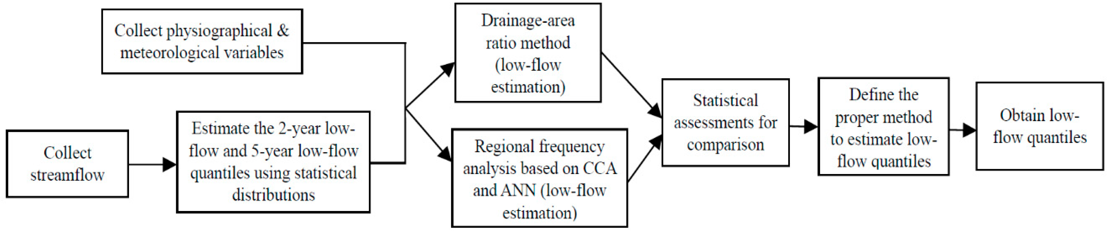
After all the variables that were used to estimate the low-flows were obtained, two methodologies, including the drainage area ratio and RFA, were applied to enhance the low-flow estimations at ungauged sites in South Korea. The drainage area ratio method uses the drainage area and low-flow quantiles. We describe this method in detail in Section 3.1. In RFA, the appropriate data preprocessing steps are required before performing the analysis. In the preprocessing stage, the physiographical, meteorological, and hydrological variables were standardized. Then, we obtained the standardized database that has a mean of zero and standard deviation of one, and asymmetry in the variables could then be assessed. With the database, RFA using CCA and ANNs were performed to estimate the low-flow quantiles in ungauged basins. We specifically describe the RFA application process and provide a diagram of the procedures that were used to obtain the low-flow estimates in Section 3.2. The overall processes that were applied in the present study are shown with a simple diagram in Figure 2.

3.1. Drainage Area Ratio Method

The drainage area ratio approach is based on the assumption that the streamflow at a location of interest can be estimated by multiplying the ratio of the drainage area corresponding to a streamflow at ungauged stations and the drainage area corresponding to a streamflow at gauged stations. The drainage area ratio approach is commonly used to estimate low-flows at ungauged locations because of its simplicity [12,29,30,31]. This method is relatively effective if the streams have similar hydrological features [32]. The method that was used in the present study is given as follows:

$$Q_y=Q_x{\left(\frac{A_y}{A_x}\right)}^m$$

(1)

where $Q_y$ denotes the estimated low-flows in the river basin of interest, $A_y$ is the basin area of the river basin of interest, $A_x$ is the basin area of the river basin with the streamflow records, and m is the exponent of $\left(A_y/A_x\right)$. In the simplest drainage ratio method, it is assumed that m equals 1 and the equation is unbiased, indicating that the expected value of the estimated low-flows tends to equal the value of the observed low-flows.

3.2. Ensemble ANN for RFA

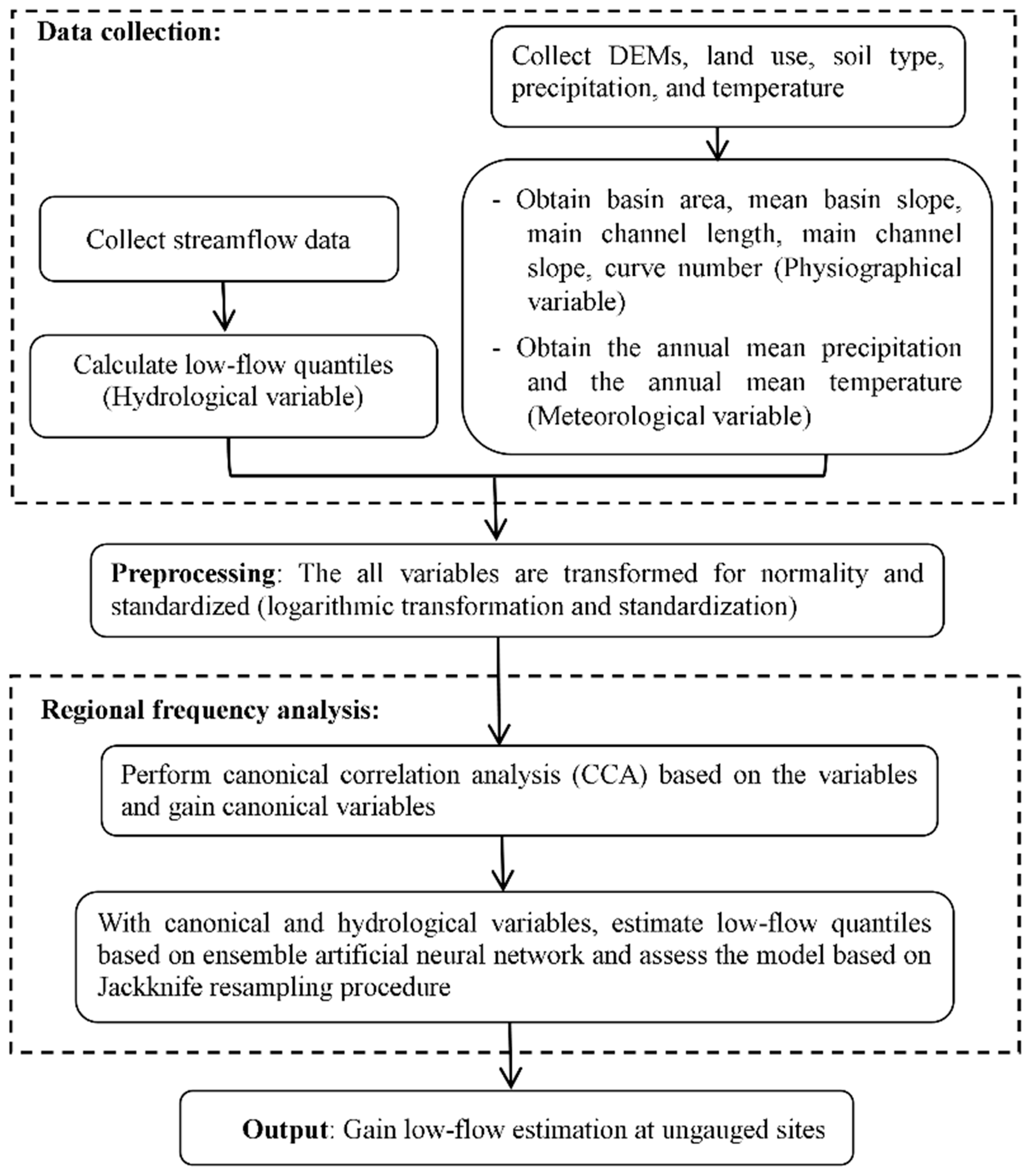
The ANNs that were used to conduct the RFA have been applied to estimate extreme events in several studies. For example, Shu and Ouarda [23] used an ensemble ANN with a CCA to improve the flood quantile estimation for extremely high flow events based on 151 catchments with ungauged sites and Ouarda and Shu [3] analyzed the low-flow quantiles of extreme events using an ensemble ANN based on more than 100 river basins in Canada. In the present study, the RFA method that was implemented to estimate the low-flows at ungauged sites in South Korea was based on the CCA and ANN methods. Using the CCA, we could construct the physiographical space as a canonical space to interpolate the hydrological variables of interest in the space, estimate the hydrological variables at ungauged sites, and create canonical variables. The canonical variables that were obtained from CCA were then fed to the ANN models to generate hydrological variable estimates in the physiographical domain. In Figure 3, a simple diagram shows the processes that were used to estimate hydrological variables such as low-flow quantiles using the CCA and ANN models.

The CCA method is a statistical multivariate analysis method that reflects the relationship between two sets of random variables by omitting nonessential data and preserving the original characteristics of the variables [33,34]. Given that we have a set of physiographical and meteorological variables, X, and a set of hydrological variables, Y, CCA was used to link the two sets based on vectors of canonical variables. If W and V are linear combinations of X and Y, we have

$$\mathrm{W}={\mathsf{\alpha }}^{\prime }\mathrm{X}$$

(2)

$$\mathrm{V}={\mathsf{\beta }}^{\prime }\mathrm{Y}$$

(3)

where W represents the canonical physiographical and meteorological variables and V represents the canonical hydrological variables. The correlation between W and V is estimated as follows.

$$\mathsf{\rho }=\frac{{\alpha }^{\prime }{\sum }_{XY}\beta }{\sqrt{{\alpha }^{\prime }{\sum }_X\alpha }\sqrt{{\beta }^{\prime }{\sum }_Y\beta }}.$$

(4)

In the CCA processes, we identified vectors $\mathsf{\alpha }$ and $\mathsf{\beta }$ by maximizing the correlation $\mathsf{\rho }$ as discussed in previous studies [18,23]. After the first pair of canonical variables were obtained, other pairs of canonical variables were calculated based on the correlation subject to the constraint of the unit variance for normalization.

The CCA in the RFA was used to construct a transformed space (canonical space) which was determined by the physiographical and meteorological characteristics of the variables and a canonical space in which the hydrological variables that are continuous can be obtained [35]. The hydrological variables can be indirectly estimated in space by establishing a functional relationship between the physiographical and meteorological variables and the hydrological variables. The physiographical and meteorological variables that are generally available at ungauged locations can provide information to calculate the hydrological variables at the ungauged sites. Thus, we can estimate hydrological variables by locating an ungauged site of interest in the canonical space defined by the variables. Additional detailed theoretical information about the application of CCAs for RFAs can be found in the study of Ouarda et al. [18]. Note that the study of Ouarda et al. [18] proposed a theoretical framework for the application of the CCA for RFAs. In the present study, the CCA was used to estimate low-flow quantiles for ungauged locations based on the ANN-based model. Also, the DAR method was applied to the study region and the results of the DAR were compared with the results of the ANN model to determine a better approach for low-flow estimation in South Korea.

In this study, ANN models were applied in canonical space to estimate the hydrological variables, such as low-flow quantiles, for ungauged basins in South Korea. Based on the CCA, the canonical variables W and V can be obtained as the linear combination of the set of physiographical and meteorological variables and the set of hydrological variables. After we obtained the canonical variable W, the ANN models were used to approximate the functional relationship between W and the hydrological variable Y. With these variables, multilayer perceptrons (MLPs), which are also known as multilayer feed-forward networks, were used to train the hydrological variables in the ANN procedure. The MLPs consist of an input layer, with one or more hidden layers, and an output layer that are interconnected. The MLP input layer receives values of the input variables and the hidden layers between the input and output layers play significant roles in transferring information between these layers. The transfer functions of the hidden layers affect the behavior of the ANN model. The output layer then provides an ANN prediction and represents the model output, which is the low-flow estimate in the present study.

The ANNs should be trained in the estimation phase using the samples from the gauged locations. During the training process of ANNs, network parameters such as the number of neurons in the hidden layer and learning rate must be optimized until the estimation error of the network is minimized and the network reaches the specified level of accuracy for the ANN model. After a network is trained and tested, the new input information can be provided to produce the model output. The training algorithm that was used in this study is the Levenberg-Marquardt (LM) algorithm. This algorithm is faster than other algorithms, such as the gradient descent method, in finding optimal solutions [36,37,38]. In the LM algorithm, an appropriate value of the scalar parameter $\mathsf{\mu }$ should be selected [39]. A large $\mathsf{\mu }$ value forces the LM algorithm to follow the gradient descent method with a small sized step, whereas a small $\mathsf{\mu }$ value leads to the Guess-Newton method, which is accurate near a minimum error solution. The initial value was given as 0.005, and the value of $\mathsf{\mu }$ changed during the ANN training process until the performance of the ANN was satisfactory. In the process, when the training epoch decreases the function of the performance, the μ value is multiplied by 0.1, whereas when the training epoch increases the function of the performance, the μ value is multiplied by 10. The maximum μ value is 10⁶, at which point the training algorithm stops. In the analysis of the ANN with the scalar parameter, an early stopping criterion was used to avoid overfitting (overtraining) during ANN training as described by Bishop [40].

To improve the generalizability and stability of the ANN, an ensemble ANN model was used in the present study. The ensemble ANN model consisted of a set of ANNs that were trained for the same task and produced the output of the model. The bagging method was applied for the ensemble ANN model to provide component networks by averaging the resulting networks. In the bagging method, each member ANN of the ensemble was trained with a subset of the training set and the subset was drawn from the original training set with replacement. This approach assists in enhancing the accuracy of the predictions and the model generalization ability in regression and classification problems [41,42,43]. Selecting the size of an ensemble plays an important role in obtaining satisfactory output from ANN models. The improvement of the generalizability is not apparent if the ensemble size is too small and the training time and ensemble creation will have time costs if this value is too large. 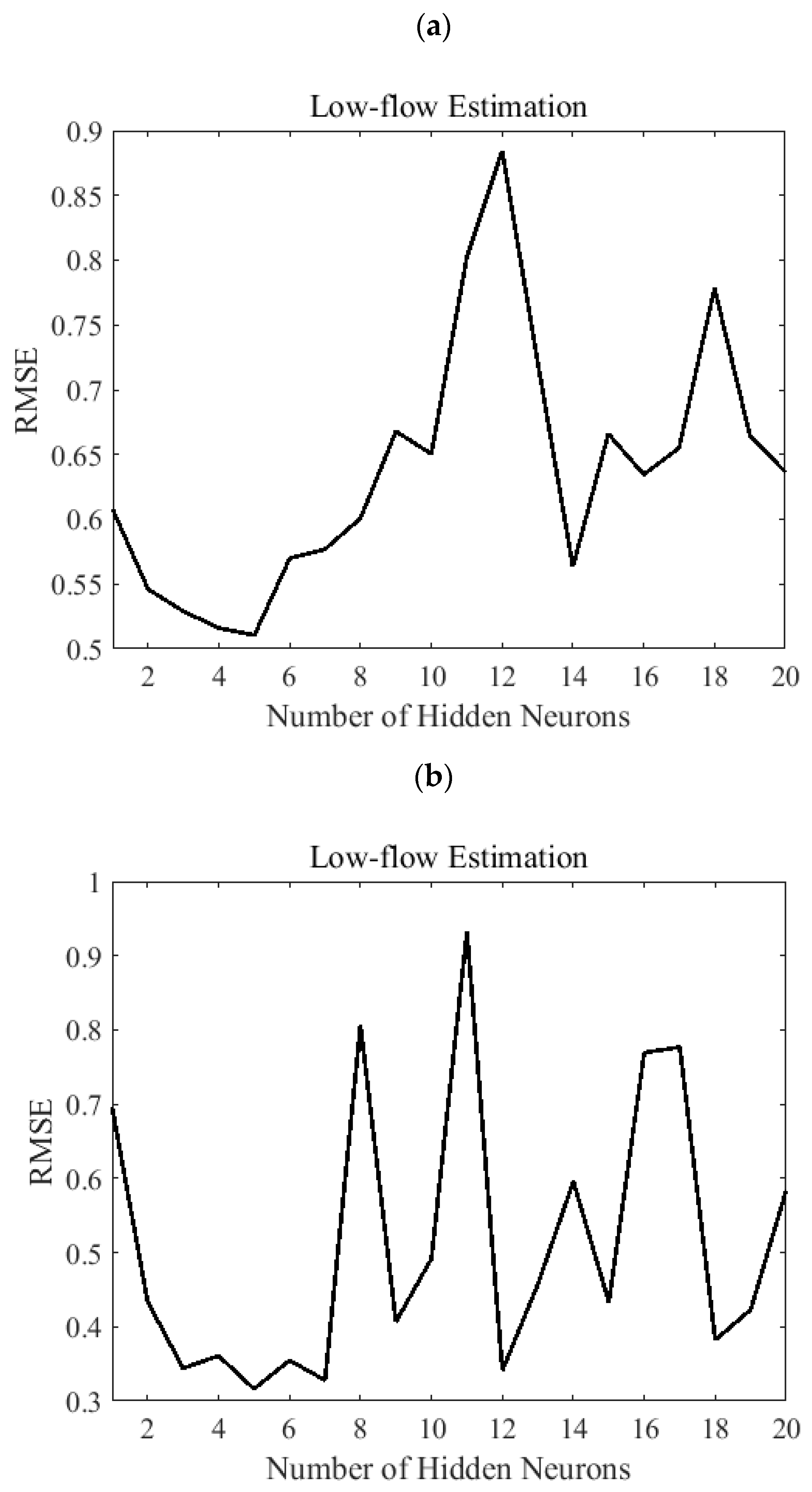Different ensemble sizes ranging from two to 20 were considered for the study area to determine the ideal number, as demonstrated in a previous study [23]. The ensemble size of 14 was chosen in this study based on the characteristics of the ensemble and hydrological variables.

3.3. Evaluation Criteria

To assess the proposed methods in the present work, we used the following indices: the R-squared (R²), mean bias (BIAS), and root mean squared error (RMSE) indices. These indices were calculated based on the following equations:

$$R^2=1-\frac{RSS}{TSS}$$

(5)

$$\mathrm{BIAS}=\frac{1}{n}{\displaystyle \sum }_{i=1}^n\left(q_i-{\widehat{q}}_i\right)$$

(6)

$$\mathrm{RMSE}=\sqrt{\frac{1}{n}{\displaystyle \sum }_{i=1}^n{\left(q_i-{\widehat{q}}_i\right)}^2}$$

(7)

where RSS is the residual sum of squares, TSS is the total sum of squares, n is the total number of sites, $q_i$ is the at-site estimate for site i, and ${\widehat{q}}_i$ is the estimate that was derived from the models for site i.

In the evaluation procedure, we use the jackknife resampling technique to compare the relative performance of each model that was used to estimate the low-flow quantiles at ungauged locations. In this procedure, the low-flow records in each drainage basin were temporarily removed from the database to assume that the site represented an ungauged location. Each model was calibrated using the data from the remaining sites. Then, regional estimates could be obtained for the ungauged river basins based on the calibrated models that were proposed in the study, and these estimates were compared to the at-site estimates, which were also called local estimates.

4. Results and Discussion

4.1. Analysis of the Correlation Between Variables

Two approaches, the drainage area ratio and RFA, were applied to obtain low-flow estimates at gauged sites in South Korea. In the first method, we used AREA with low-flow quantiles of a two-year return period and a five-year return period and in the second method, we used AREA, MBS, AMT, AMT, MCL, MCS, and CN with these low-flow quantiles.

The physiographical and meteorological variables that were considered in this study were investigated to identify correlations with the hydrological variables, the two-year low-flow quantile, and the five-year low-flow quantile, as defined by statistical distributions. The scatterplots between (a) the two-year quantile and (b) the five-year quantile that were estimated from the Gamma distribution and the physiographical and climatic variables are presented in Figure 4.

The two-year low-flow quantile plot shows that the river basin descriptors, including AREA, MBS, MCL, CN, and AMP, are positively correlated with low-flows and the other river basin descriptors, namely MCS and AMT, are negatively correlated with low-flows. For the five-year low-flow quantile plot, the observations are similar, except for the MBS. The MCS exhibits a positive correlation with low-flows when divided by the basin area to offset the area effect. The Pearson correlation coefficients of variables range from 0.063 to 0.491 for the two-year quantile and from 0.137 to 0.498 for the five-year quantile. In the RFA process, we used the canonical correlation coefficients, as described in the methodology section. Thus, we also examined the canonical correlation coefficients for the variables to determine the improvements in the correlations between the variables when CCA was applied. The canonical correlation coefficients range from 0.161 to 0.889 for the two-year quantile and from 0.124 to 0.883 for the five-year quantile, as shown in Table 3. In particular, the canonical correlation coefficients for the two-year quantile are high for AREA, MCL, AMP, and AMT compared to the corresponding Pearson correlation coefficients.

We also tested the hypothesis that there is no relationship between the physiographical and meteorological variables and the hydrological variables. Based on the test, the corresponding correlations between AREA, AMP, MCL, and MCS and low-flows were considered significant at the 95% confidence level. The corresponding correlations between MBS, AMT, and CN and low-flows were not considered significant at the 95% confidence level. However, MBS and AMT positively affected the model’s performance in estimating the low-flows at ungauged sites based on RFA, potentially because AMT is highly related to AMP, and the corresponding correlation between MBS and AMT was considered significant at the 95% confidence level. The combinations of the variables that were used in the RFA processes may have also influenced the model’s performance.

4.2. Analysis of the Drainage Area Ratio Method

To estimate the low-flows at ungauged sites in South Korea, the drainage area ratio method was generally used based on the river basin area. In this study, one river basin was considered a gauged site and the other river basins were considered ungauged sites. For example, if the Imokjeonggyo station was used as the gauged location, the low-flow estimates in other river basins were obtained using Equation (1).

Table 4. Validation results using the drainage-area ratio method for the two-year and five-year low-flow quantiles.

River Name	Two-Year Return Period			Five-Year Return Period
	BIAS	RMSE	R2	BIAS	RMSE	R2
Imokjeonggyo	−1.888	3.539	0.111	−1.130	2.097	0.044
Baekokpogyo	−6.171	9.933	0.141	−2.655	4.358	0.054
Youngyang	0.322	0.809	0.117	0.355	0.570	0.046
Cheongsong	0.600	0.855	0.117	0.291	0.542	0.047
Donggok	−1.009	2.270	0.111	0.129	0.547	0.042
Goro	−1.624	3.154	0.115	0.119	0.551	0.043
Epyunggyo	−3.171	5.440	0.112	−0.790	1.606	0.043
Tanbugyo	0.075	0.939	0.109	0.018	0.609	0.042
Gidaegyo	0.435	0.802	0.119	0.267	0.536	0.047
Soyanggang Dam	0.667	0.895	0.149	0.396	0.596	0.113
Goesan Dam	0.104	0.917	0.119	−0.020	0.639	0.047
Andong Dam	0.681	0.904	0.151	0.415	0.609	0.077
Imha Dam	0.787	0.989	0.169	0.421	0.614	0.072
Hapcheon Dam	0.316	0.811	0.118	0.197	0.532	0.049
Wonju	−0.105	1.105	0.111	−0.089	0.702	0.044
Dopyeong	−2.739	4.797	0.126	−1.320	2.375	0.051
Imgye	−0.507	1.584	0.115	−0.211	0.835	0.046
Maeil	−0.272	1.292	0.115	0.115	0.552	0.045
Toegyewon	−0.361	1.400	0.116	−0.173	0.791	0.047
Jungnanggyo	−3.390	5.767	0.148	−3.110	5.039	0.081
Gyeongan	−1.245	2.605	0.126	−1.021	1.938	0.055
Heukcheongyo	−0.734	1.888	0.116	−0.110	0.724	0.045
Hoengseong	−0.419	1.472	0.122	−0.264	0.898	0.050
Hwachon	0.095	0.924	0.120	−0.011	0.631	0.049
Chungmi	0.060	0.951	0.120	0.102	0.558	0.049
Pyeong Chang	−0.698	1.839	0.119	−0.546	1.265	0.042
Misung	−0.042	1.042	0.114	0.166	0.536	0.044
Hyoryeong	0.497	0.813	0.111	0.192	0.532	0.044
Cheoncheon	−0.456	1.520	0.119	−0.176	0.794	0.048
Gosan	−1.921	3.589	0.135	−0.619	1.366	0.051
Cheongseon2	0.141	0.891	0.071	0.028	0.602	0.019
Yeongwol	−0.817	2.002	0.126	−0.140	0.755	0.049
Banglimgyo	−0.412	1.463	0.111	−0.610	1.353	0.039

shows the assessment of the drainage area ratio method based on the BIAS, RMSE, and R² values using the two-year quantile and the five-year quantile derived from Gamma distribution. BIAS values range from −6.171 to 0.787; RMSE values range from 0.802 to 9.933; and R² values range from 0.071 to 0.169 for the two-year quantile. Additionally, BIAS values range from −3.110 to 0.421; RMSE values range from 0.532 to 5.039; and R² values range from 0.019 to 0.113 for the five-year quantile.

Figure 5 plots the relationship between the estimated low-flow using the drainage area ratio method and the measured low-flow based on the two-year quantile of the Gamma distribution for the river basins that were used in this study. We only show the results in Figure 5 based on the two-year quantile derived from the Gamma distribution because other distributions with these quantiles displayed similar results. The subfigures in Figure 5 represent the following selected stations: 1. Imokjeonggyo, 2. Baekokpogyo, 3. Youngyang, 4. Cheongsong, 5. Donggok, 6. Goro, 7. Epyunggyo, 8. Tanbugyo, 9. Gidaegyo, 10. Soyanggang Dam, 11. Goesan Dam, 12. Andong Dam, 13. Imha Dam, 14. Hapcheon Dam, 15. Wonju, 16. Dopyeong, 17. Imgye, 18. Maeil, 19. Toegyewon, 20. Jungnanggyo, 21. Gyeongan, 22. Heukcheongyo, 23. Hoengseong, 24. Hwachon, 25. Chungmi, 26. Pyeong Chang, 27. Misung, 28. Hyoryeong, 29. Cheoncheon, 30. Gosan, 31. Cheongseon 2, 32. Yeongwol, and 33. Banglimgyo. A limitation of linear methods is that they provide biased estimates in the flood flow domain [44], and this phenomenon was observed in the present work, as shown in Figure 5. Also, Pandey and Nguyen [45] and Grover et al. [46] stated that non-linear approaches can produce more precise estimates than linear regression methods in RFA procedures. If the area of the river basin with streamflow records is too large in the drainage area ratio method, the low-flows are underestimated (e.g., Soyanggang Dam, Andong Dam, and Imha Dam). Conversely, when the area of the basin with the streamflow records is too small, the low-flows are overestimated (e.g., Imokjeonggyo, Baekokpogyo, and Epyunggyo). Based on the BIAS and RMSE results that were obtained from the drainage area ratio approach, we chose Misung station and compared the results with the indices that were calculated by RFA to estimate the low-flow quantiles at ungauged locations in South Korea.

4.3. RFA with CCA and ANNs

In estimating the low-flow quantiles based on RFA, identifying the number of hidden neurons in the hidden layers is a significant task to improve model performance. In general, if too many hidden neurons are used, overfitting can occur due to not having enough training cases in the ensemble ANN process. If too few neurons are used, underfitting can occur due to not having sufficient complexity to represent the functional relationship between the input and output systems [3,23]. For comparison with the drainage area ratio method that was used to calculate the low-flow quantiles at ungauged sites in South Korea, we performed RFA with CCA-based ANNs using the low-flow quantiles defined by the Gamma distribution. By varying the number of hidden neurons from one to 20, as shown in Figure 6, we can observe that the ensemble ANN models for the two-year quantile and five-year quantile suffer from overfitting problems when the number of hidden neurons increases above five hidden neurons. The ensemble ANN models with five hidden neurons tend to provide the most reliable estimates of low-flows at ungauged sites; therefore, we selected the five hidden neurons for low-flow estimation in this study. The performance measure, RMSE, was obtained from a jackknife procedure to identify the optimal number of hidden neurons. Note that we also compared the ensemble ANN-based model without the CCA and with the CCA to identify the impact of the CCA on the proposed model. The model without the CCA was built using AMP, which is the most highly correlated variable with the low-flow in this study. The results for the model performance are presented in Table 5. This table indicates that the CCA-based model (the ensemble ANN model with CCA) seems to provide a better performance based on the RMSE, BIAS, and R² indices.

Based on the optimal number of hidden neurons for the ensemble ANN models based on the CCA, we obtained RMSE, BIAS, and R² values for the results of the RFA using the two-year and five-year quantiles and compared these values with the results of the drainage area ratio method. Table 5 presents the results that were obtained from the drainage area ratio method and the ensemble ANN model using the jackknife validation procedure. For each cell in this table, a bold font denotes the best performing method for the low-flow estimation. Table 6a indicates that RFA with the ensemble ANN model provides better performance than the drainage area ratio approach based on the indices for the two-year quantile low-flows. In Table 6b, the RFA with the ensemble ANN model is compared with the drainage area ratio method for the five-year low-flow quantile. Based on statistical assessments, the model performance is relatively high when the RFA was used to obtain the low-flow estimates at ungauged sites. Thus, the ensemble ANN model, which is a nonlinear method, yields a performance enhancement. In particular, the ensemble ANN model improves the bias problem, which is highly important in the design of hydrological structures.

The regional estimates of low-flow using the jackknife validation procedure for the drainage area ratio method and RFA based on the ensemble ANN model are shown in Figure 7a for the two-year quantile and Figure 7b for the five-year quantile derived from the Gamma distribution. This figure shows that the ensemble ANN model typically exhibits better performance than the drainage area ratio approach at Misung station. This result indicates that the ensemble ANN, as a nonlinear model, outperforms the drainage area ratio method, as a linear model, for the two quantiles. A similar study was performed for river basins in Canada to obtain low-flow quantiles by comparing models based on the ANN and multiple regression methods [3]. In their analysis, the ANN-based model also led to a better performance compared with the regression models. The ensemble ANN model provides less biased estimates and better prediction accuracy than the drainage area ratio method. The BIAS, RMSE, and R² values of the drainage area ratio method are −0.042, 1.042, and 0.114, respectively, for the two-year quantile. Additionally, the BIAS, RMSE, and R² values of RFA are 0.013, 0.511, and 0.408, respectively, for the two-year quantile. Moreover, these indices for the five-year quantile are 0.166, 0.536, and 0.044 and −0.018, 0.316, and 0.573 based on the drainage area ratio method and RFA, respectively. Figure 7 shows that for the drainage area ratio approach, most of the low-flows are underestimated. However, using RFA, the bias problem is adjusted and the accuracy is improved for both quantiles, as shown in Figure 7.

To evaluate the low-flow estimates based on the Gamma distribution, different statistical distributions were used by creating the two-year and five-year quantiles. The regional estimates of the low-flows based on GEV, L2, and W2 using the jackknife validation procedure are plotted against the local estimates in Figure 8. The figure indicates that the regional estimates of the low-flows derived from GEV, L2, and W2 are similar to the regional estimates of the low-flows using the Gamma distribution. Based on Gamma distribution results, the results of RFA based on the three distributions exhibit better performance than those of the drainage area ratio method for the two-year low-flow and the five-year low-flow quantiles shown in Figure 8.

The indices, including BIAS, RMSE, and R², for the Gamma, GEV, L2, and W2 distributions are shown in Table 7. The Gamma distribution exhibits the highest accuracy in estimating the low-flow quantiles based on the RMSE and R² values. The W2 distribution displays the best bias values for the two-year and five-year quantiles. However, all the distributions that were used in this study yielded good bias values and they improved the bias problem compared to using the drainage area ratio method.

5. Conclusions

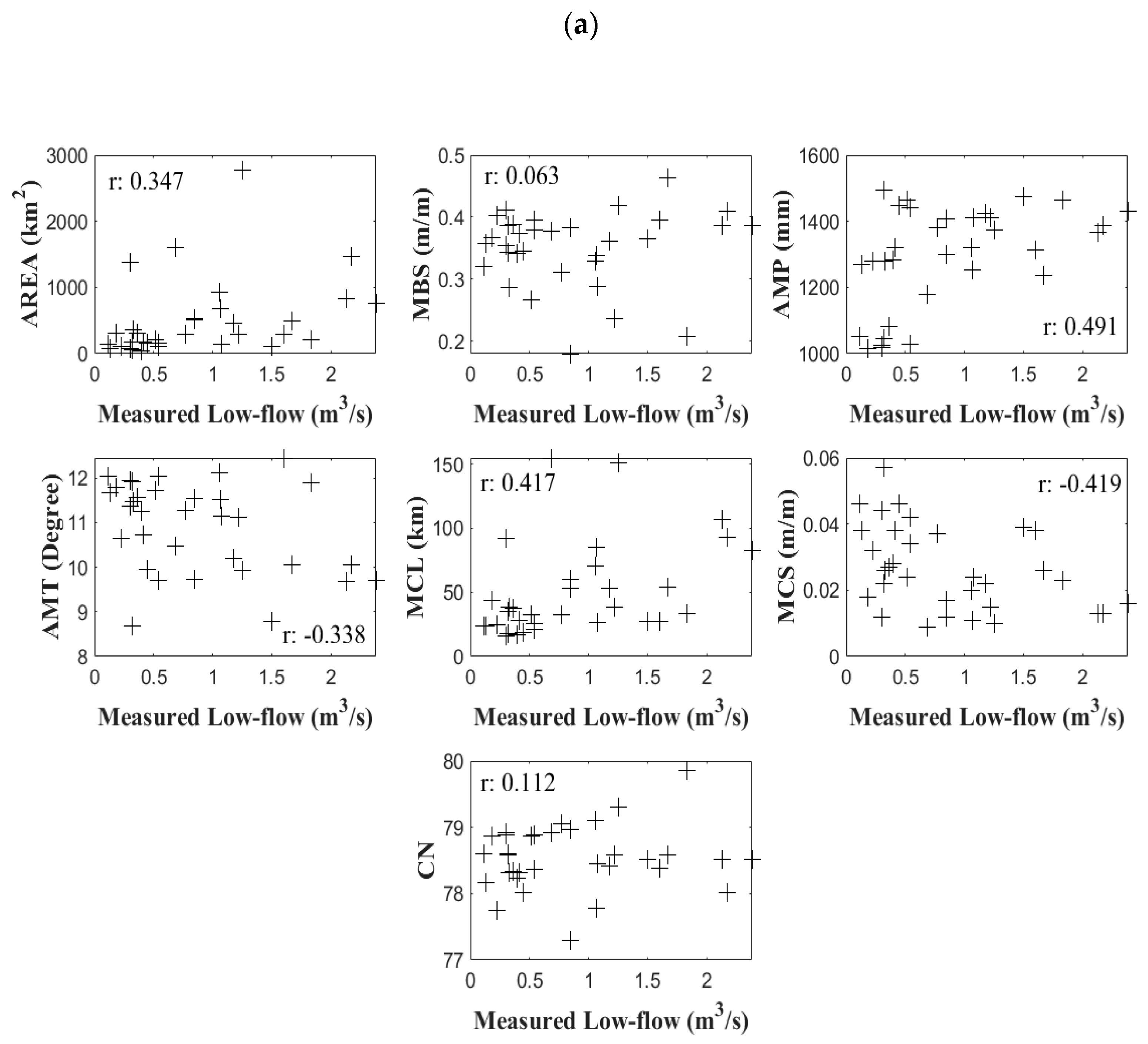
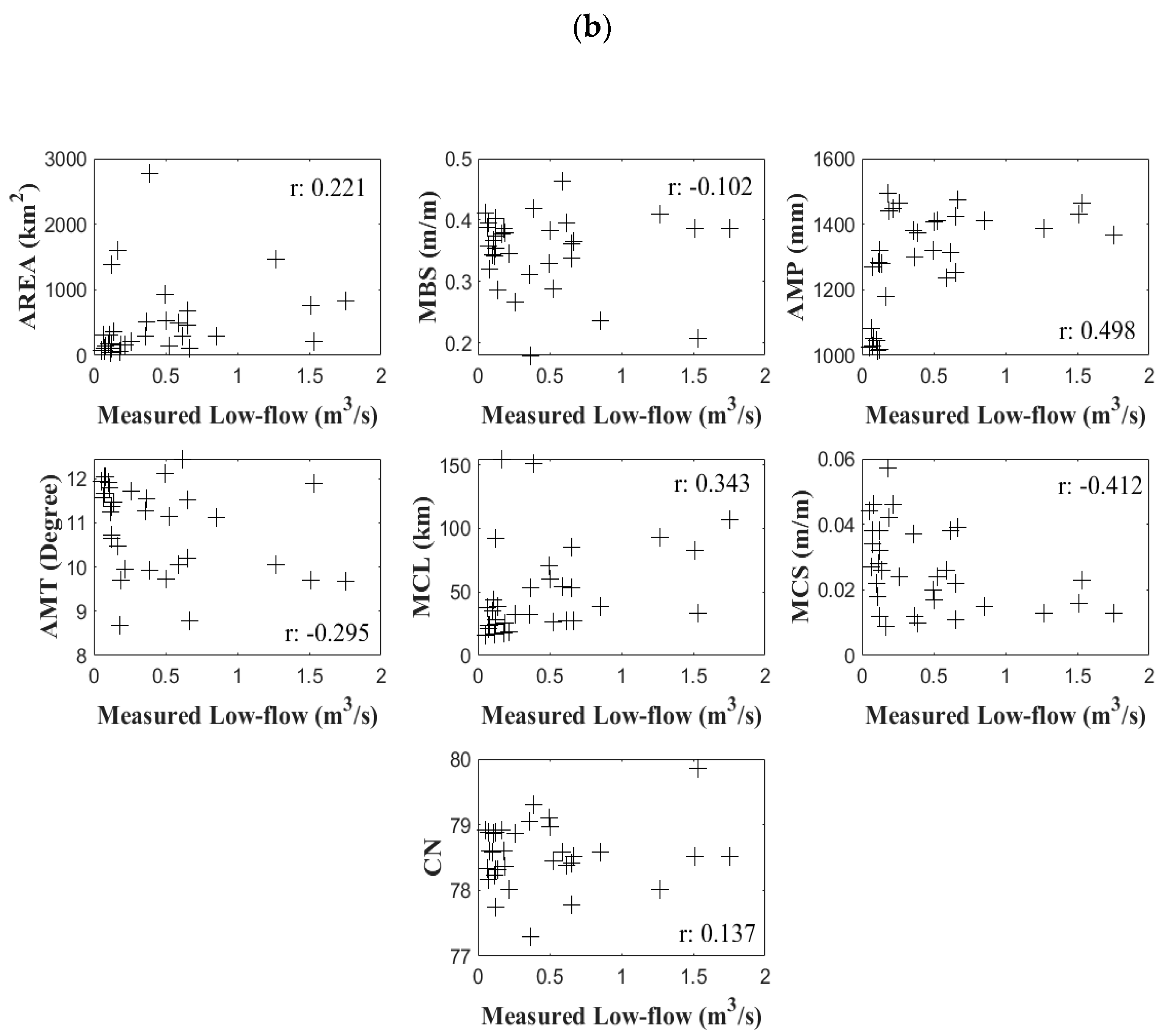
We examined the correlations between the physiographical/meteorological variables and the hydrological variables to better understand the characteristics of low-flows. Among the variables representing the physiographical and climatic features, we found that AREA, AMP, MCL, and MCS are positively correlated with low-flows based on a significance test. Additionally, MBS, AMT, and CN are not significantly correlated with low-flows, but are correlated with other variables that may influence the RFA results. In addition, when we used CCA to generate the canonical correlation coefficients of the variables, the correlations between the physiographical/meteorological variables and low-flows were improved.

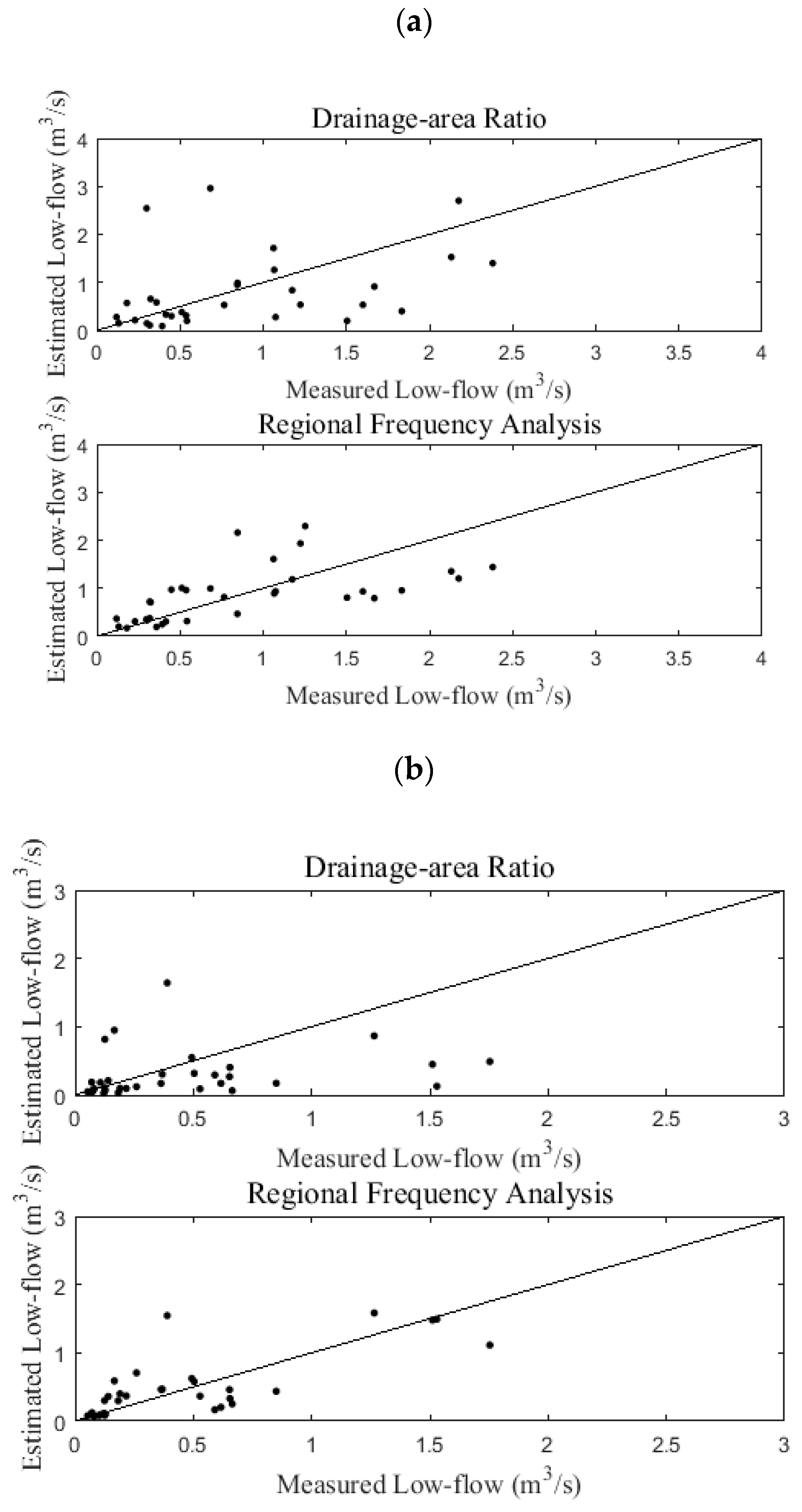
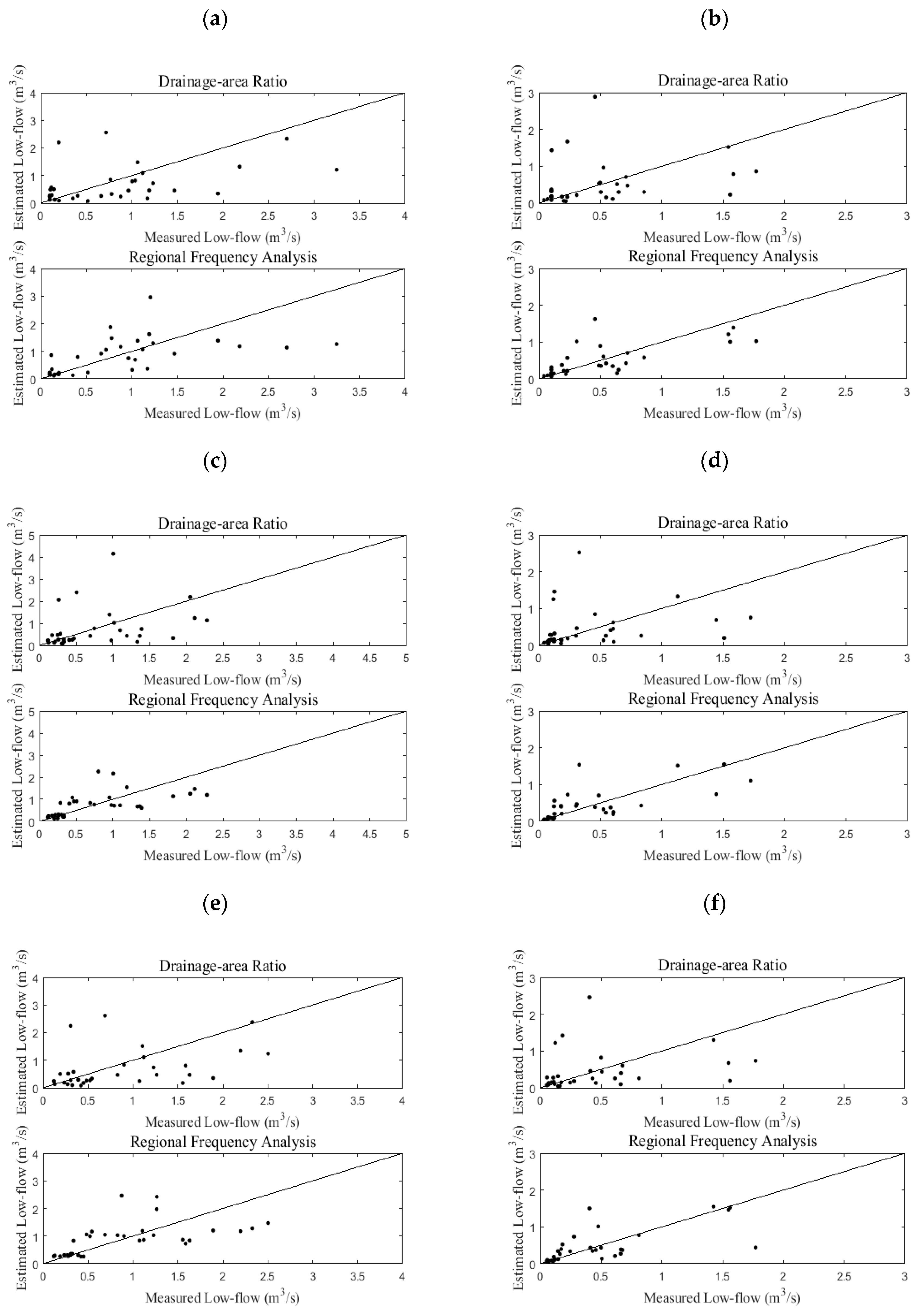
The drainage area ratio method was used to estimate the low-flows at ungauged sites. With this method, one river basin was considered a gauged basin and the other basins were considered ungauged basins. Using the basin area ratio, the method was assessed based on the BIAS, RMSE, and R². The average values of BIAS, RMSE, and R² were −0.703, 2.097, and 0.121 for the two-year quantile and −0.297, 1.111, and 0.050 for the five-year quantile, respectively. To compare the results of the drainage area ratio method and RFA, several basins that exhibited good performance were selected. The ranges of the BIAS, RMSE, and R² values of the Misung, Tanbugyo, Chungmi, and Hwachon basins were −0.042~0.095, 0.924~1.042, and 0.109~0.120 for the two-year quantile and −0.011~0.166, 0.536~0.631, and 0.042~0.049 for the five-year quantile, respectively. Additionally, if the selected basin was too small or too large, the estimated quantiles were biased. Based on the results of this study, the estimates seem to be relatively overestimated when the basin area is smaller than 150 km² and relatively underestimated when the basin area is larger than 1000 km².

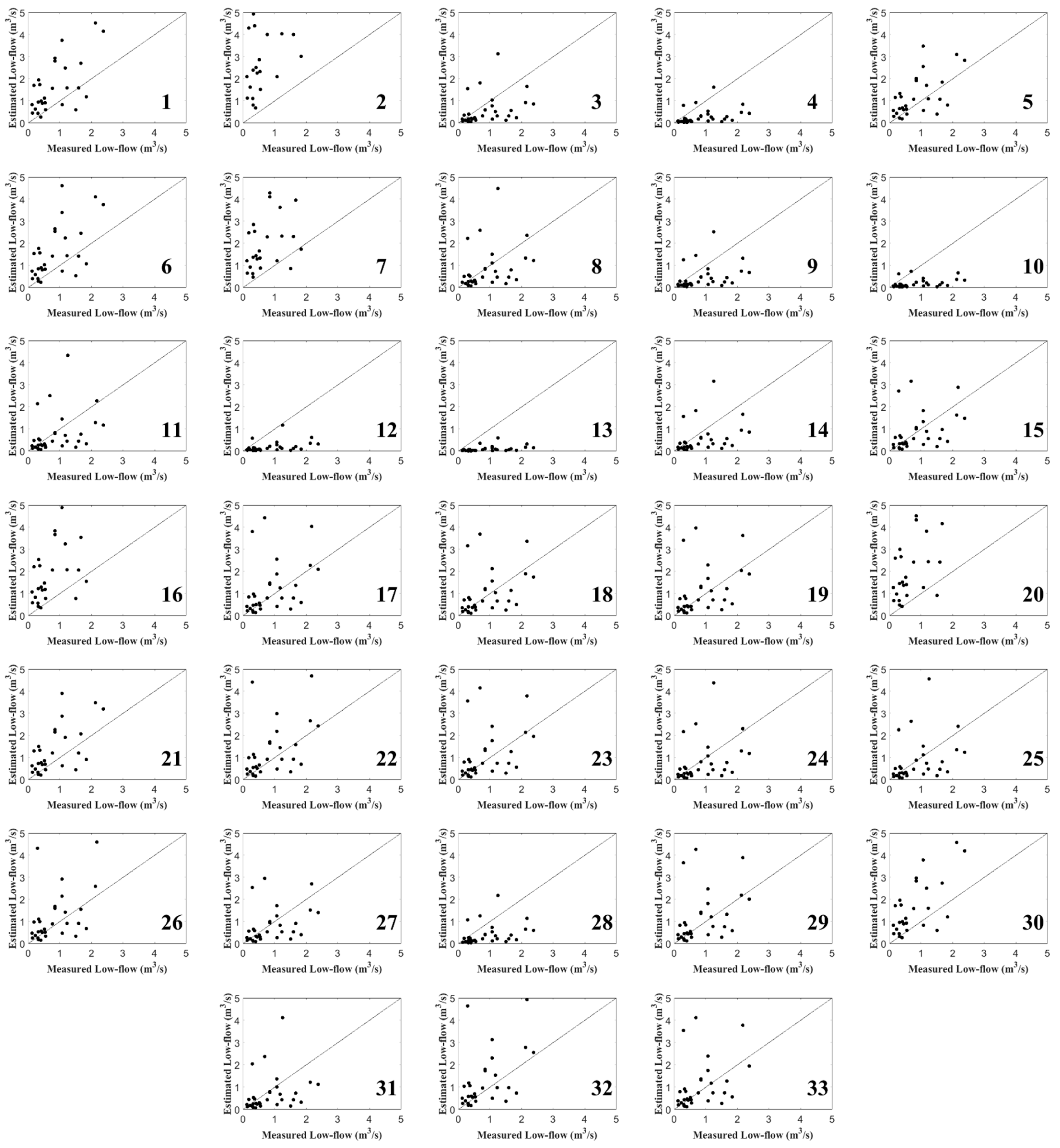
Compared with the drainage area ratio approach, RFA using CCA-based ANNs was applied for the 33 river basins. In this assessment, we used jackknife validation with statistical indices, such as BIAS, RMSE, and R². The indices based on the RFA were 0.013, 0.511, and 0.408 for the two-year quantile and −0.018, 0.316, and 0.573 for the five-year quantile. Based on the indices, we found that the RFA method that was proposed in this paper performs better than the drainage area ratio method based on the results for the 33 river basins. We determine that the ensemble ANN method, as a nonlinear model, seems to outperform the drainage area ratio approach, a linear model, in obtaining low-flow estimates at ungauged sites in South Korea. Although the ensemble ANN did not show such improvements, we found that the nonlinear model has the potential to enhance low-flow estimations in the study region.

Other statistical distributions, such as GEV, LN2, and W2, were used to obtain the two-year and five-year low-flow quantiles and to assess the low-flow estimates at ungauged basins. When these distributions are used in RFA and the drainage area ratio method, RFA based on CCA and ANNs outperforms the drainage area ratio approach, and the Gamma distribution provides the best results. The BIAS, RMSE, and R² values are also used for model assessment based on the distributions. W2 exhibits the best performance for BIAS and the Gamma distribution displays the best performance for RMSE and R². In this paper, we found that the machine learning-based nonlinear model provides relatively reliable estimates of low-flow quantiles for ungauged basins in South Korea compared to the estimates by the linear model. The results point to the use of the machine learning model to enhance estimates of low-flow quantiles in areas characterized by nonlinearity. Additionally, the explicit correlations between the quantiles and the sets of physiographical and meteorological covariates can be determined to improve the quality of regional quantile estimates in ungauged basins.

References

1. Fiala, T.; Ouarda, T.B.M.J.; Hladný, J. Evolution of low flows in the Czech Republic. J. Hydrol. 2010, 393, 206–218. [Google Scholar] [CrossRef]
2. Kroll, C.; Luz, J.; Allen, B.; Vogel, R.M. Developing a watershed characteristics database to improve low streamflow prediction. J. Hydrol. Eng. 2004, 9, 116–125. [Google Scholar] [CrossRef]
3. Ouarda, T.B.M.J.; Shu, C. Regional low-flow frequency analysis using single and ensemble artificial neural networks. Water Resour. Res. 2009, 45. [Google Scholar] [CrossRef]
4. Smakhtin, V.U. Low flow hydrology: A review. J. Hydrol. 2001, 240, 147–186. [Google Scholar] [CrossRef]
5. Brutsaert, W.; Nieber, J.L. Regionalized drought flow hydrographs from a mature glaciated plateau. Water Resour. Res. 1977, 13, 637–643. [Google Scholar] [CrossRef]
6. Chapman, T.G. Modelling stream recession flows. Environ. Model. Softw. 2003, 18, 683–692. [Google Scholar] [CrossRef]
7. Wittenberg, H. Nonlinear analysis of flow recession curves. IAHS Publ. 1994, 221, 61–68. [Google Scholar]
8. Kang, K.-S.; Seoh, B.-H. Analysis of droughts for hydrological design of reservoirs at dam sites. J. Korean Soc. Civ. Eng. 1995, 2, 149–152. [Google Scholar]
9. Wiche, G.J.; Benson, R.D.; Emerson, D.G. Streamflow at Selected Gaging Stations on the James River in North Dakota and South Dakota, 1953-82, with a Section on Climatology; US Geological Survey. Water Resour. Investig. Rep.: Reston, VA, USA, 1989.
10. Guenthner, R.S.; Weigel, J.F.; Emerson, D.G. Gaged and Estimated Monthly Streamflow during 1931-84 for Selected Sites in the Red River of the North Basin in North Dakota and Minnesota; US Geological Survey, Water Resour. Investig. Rep.: Reston, VA, USA, 1990.
11. Emerson, D.G.; Dressler, V.M. Historic and Unregulated Monthly Streamflow for Selected Sites in the Red River of the North Basin in North Dakota, Minnesota, and South Dakota, 1931-99; US Geological Survey, Water Resour. Investig. Rep.: Reston, VA, USA, 2002.
12. Cho, T.-G.; Lee, K.-S.; Kim, Y.-O. Improving low flow estimation for ungauged basins in Korea. J. Korea Water Resour. Assoc. 2007, 40, 113–124. [Google Scholar] [CrossRef]
13. Beable, M.E.; McKerchar, A.I. Regional flood estimation in New Zealand. Water Soil Tech. Publ. 1982, 20, 139. [Google Scholar]
14. Matalas, N.C.; Slack, J.R.; Wallis, J.R. Regional skew in search of a parent. Water Resour. Res. 1975, 11, 815–826. [Google Scholar] [CrossRef]
15. Burn, D.H. Evaluation of regional flood frequency analysis with a region of influence approach. Water Resour. Res. 1990, 26, 2257–2265. [Google Scholar] [CrossRef]
16. Haddad, K.; Rahman, A. Regional flood frequency analysis in eastern Australia: Bayesian GLS regression-based methods within fixed region and ROI framework–Quantile Regression vs. Parameter Regression Technique. J. Hydrol. 2012, 430, 142–161. [Google Scholar] [CrossRef]
17. Zrinji, Z.; Burn, D.H. Flood frequency analysis for ungauged sites using a region of influence approach. J. Hydrol. 1994, 153, 1–21. [Google Scholar] [CrossRef]
18. Ouarda, T.B.M.J.; Girard, C.; Cavadias, G.S.; Bobee, B. Regional flood frequency estimation with canonical correlation analysis. J. Hydrol. 2001, 254, 157–173. [Google Scholar] [CrossRef]
19. Luk, K.C.; Ball, J.E.; Sharma, A. An application of artificial neural networks for rainfall forecasting. Math. Comput. Model. 2001, 33, 683–693. [Google Scholar] [CrossRef]
20. Shu, C.; Burn, D.H. Artificial neural network ensembles and their application in pooled flood frequency analysis. Water Resour. Res. 2004, 40. [Google Scholar] [CrossRef]
21. Dawson, C.W.; Abrahart, R.J.; Shamseldin, A.Y.; Wilby, R.L. Flood estimation at ungauged sites using artificial neural networks. J. Hydrol. 2006, 319, 391–409. [Google Scholar] [CrossRef]
22. Seidou, O.; Ouarda, T.B.M.J.; Bilodeau, L.; Hessami, M.; St-Hilaire, A.; Bruneau, P. Modeling ice growth on Canadian lakes using artificial neural networks. Water Resour. Res. 2006, 42. [Google Scholar] [CrossRef]
23. Shu, C.; Ouarda, T.B.M.J. Flood frequency analysis at ungauged sites using artificial neural networks in canonical correlation analysis physiographic space. Water Resour. Res. 2007, 43. [Google Scholar] [CrossRef]
24. Kendall, M.G. Rank Correlation Methods; Charles Griffin & Co. Ltd.: London, UK, 1948. [Google Scholar]
25. Wald, A.; Wolfowitz, J. An exact test for randomness in the non-parametric case based on serial correlation. Ann. Math. Stat. 1943, 14, 378–388. [Google Scholar] [CrossRef]
26. Mosaffaie, J. Comparison of two methods of regional flood frequency analysis by using L-moments. Water Resour. 2015, 42, 313–321. [Google Scholar] [CrossRef]
27. Singh, V.P. On application of the Weibull distribution in hydrology. Water Resour. Manag. 1987, 1, 33–43. [Google Scholar] [CrossRef]
28. Chowdhury, J.U.; Stedinger, J.R.; Lu, L.H. Goodness-of-fit tests for regional generalized extreme value flood distributions. Water Resour. Res. 1991, 27, 1765–1776. [Google Scholar] [CrossRef]
29. Choquette, A.F. Regionalization of Peak Discharges for Streams in Kentucky; US Geological Survey, Water Resour. Investig. Rep.: Reston, VA, USA, 1998.
30. Koltun, G.F.; Roberts, J.W. Techniques for Estimating flood-Peak Discharges of Rural, Unregulated Streams in Ohio; US Geological Survey, Water Resour. Investig. Rep.: Reston, VA, USA, 1990.
31. Bisese, J.A. Methods for Estimating the Magnitude and Frequency of Peak Discharges of Rural, Unregulated Streams in Virginia; US Geological Survey, Water Resour. Investig. Rep.: Reston, VA, USA, 1995.
32. Hirsch, R.M. An evaluation of some record reconstruction techniques. Water Resour. Res. 1979, 15, 1781–1790. [Google Scholar] [CrossRef]
33. Razavi, A.R.; Gill, H.; Åhlfeldt, H.; Shahsavar, N. A data pre-processing method to increase efficiency and accuracy in data mining. Artif. Intell. Med. 2005, 3581, 434–443. [Google Scholar]
34. Muirhead, R.J. Aspects of Multivariate Statistical Theory, 197; John Wiley & Sons: Hoboken, NJ, USA, 2009. [Google Scholar]
35. Chokmani, K.; Ouarda, T.B.M.J. Physiographical space-based kriging for regional flood frequency estimation at ungauged sites. Water Resour. Res. 2004, 40. [Google Scholar] [CrossRef]
36. Hagan, M.T.; Menhaj, M.B. Training feedforward networks with the Marquardt algorithm. IEEE Trans. Neural Netw. 1994, 5, 989–993. [Google Scholar] [CrossRef] [PubMed]
37. Bishop, C.M. Neural Networks for Pattern Recognition; Oxford University Press: New York, NY, USA, 1995. [Google Scholar]
38. Burney, S.M.A.; Jilani, T.A.; Ardil, C. A comparison of first and second order training algorithms for artificial neural networks. In Proceedings of the International Conference on Computational Intelligence, Istanbul, Turkey, 17–19 December 2004. [Google Scholar]
39. Demuth, H.; Beale, M.; Hagan, M. Neural Network Toolbox™ 6, User’s Guide; MathWorks Inc.: Boston, MA, USA, 2008. [Google Scholar]
40. Bishop, C.M. Pattern Recognition and Machine Learning; Springer: Berlin/Heidelberg, Germany, 2006. [Google Scholar]
41. Efron, B.; Tibshirani, R.J. An Introduction to the Bootstrap; CRC Press: Boca Raton, FL, USA, 1994. [Google Scholar]
42. Cannon, A.J.; Whitfield, P.H. Downscaling recent streamflow conditions in British Columbia, Canada using ensemble neural network models. J. Hydrol. 2002, 259, 136–151. [Google Scholar] [CrossRef]
43. Carney, J.G.; Cunningham, P. The NeuralBAG algorithm: Optimizing generalization performance in bagged neural networks. In Proceedings of the ESANN, Bruges, Belgium, 21–23 April 1999. [Google Scholar]
44. McCuen, R.H.; Leahy, R.B.; Johnson, P.A. Problems with logarithmic transformations in regression. J. Hydraul. Eng. 1990, 116, 414–428. [Google Scholar] [CrossRef]
45. Pandey, G.R.; Nguyen, V.-T.-V. A comparative study of regression based methods in regional flood frequency analysis. J. Hydrol. 1999, 225, 92–101. [Google Scholar] [CrossRef]
46. Grover, P.L.; Burn, D.H.; Cunderlik, J.M. A comparison of index flood estimation procedures for ungauged catchments. Can. J. Civ. Eng. 2002, 29, 734–741. [Google Scholar] [CrossRef]
Figure 1. The 33 river basins in South Korea that were used in the study. The black points indicate the outlet of each river basin, which includes a streamflow station.
Atmosphere 10 00695 g001
Figure 2. Overall processes to obtain the hydrological variable estimation (low-flow estimation) in this study.
Atmosphere 10 00695 g002
Figure 3. Diagram of the processes that were used to obtain the low-flow estimates at ungauged locations based on regional frequency analysis.
Atmosphere 10 00695 g003
Figure 4. Correlation between physiographical and meteorological variables and (a) two-year low-flow quantile and (b) five-year low-flow quantile. r indicates the correlation coefficient for each basin.
Atmosphere 10 00695 g004aAtmosphere 10 00695 g004b
Figure 5. Plot of the estimated low-flow and measured low-flow values for the two-year quantile based on 33 river networks using the drainage-area ratio method.
Atmosphere 10 00695 g005
Figure 6. RMSE of the low-flow estimation using the ensemble artificial neural networks with the number of hidden neurons ranging from 1 to 20 for the (a) two-year quantile and (b) five-year quantile derived from the Gamma distribution.
Atmosphere 10 00695 g006
Figure 7. Plot of the estimated flow and measured flow based on the drainage-area ratio for Misung station and regional frequency analysis for the (a) two-year low-flow quantile and (b) five-year low-flow quantile derived from the Gamma distribution.
Atmosphere 10 00695 g007
Figure 8. Plot of the estimated flow and measured flow based on the drainage-area ratio and regional frequency analysis for the (a) two-year quantile and (b) five-year quantile derived from the generalized extreme value (GEV) distribution, (c) two-year quantile and (d) five-year quantile derived from the LN2 distribution and (e) two-year quantile and (f) five-year quantile derived from the W2 distribution.
Atmosphere 10 00695 g008