Article

Parallel Comparison of Major Sudden Stratospheric Warming Events in CESM1-WACCM and CESM2-WACCM

1
Key Laboratory of Meteorological Disaster, Ministry of Education (KLME)/Joint International Research Laboratory of Climate and Environment Change (ILCEC)/Collaborative Innovation Center on Forecast and Evaluation of Meteorological Disasters (CIC-FEMD), Nanjing University of Information Science & Technology, Nanjing 210044, China
2
Fredy & Nadine Herrmann Institute of Earth Sciences, The Hebrew University of Jerusalem, Edmond J. Safra Campus, Givat Ram Jerusalem 91904, Israel
*
Author to whom correspondence should be addressed.
Atmosphere 2019, 10(11), 679; https://doi.org/10.3390/atmos10110679
Submission received: 14 October 2019 / Accepted: 1 November 2019 / Published: 5 November 2019
(This article belongs to the Section Meteorology)

Abstract

:
After the recent release of the historical runs by community Earth system model version 2–the whole atmosphere community climate model (CESM2-WACCM), the major sudden stratospheric warming (SSW) events in this model and in its previous version (CESM1-WACCM) are compared based on a modern reanalysis (JRA55). Using the World Meteorological Organization (WMO) definition of SSWs and a threshold-based classification method that can describe the polar vortex morphology, SSWs in models and the reanalysis are further classified into two types, vortex displacement SSWs and vortex split SSWs. The general statistical characteristics of the two types of SSW events in the two model versions are evaluated. Both CESM1-WACCM and CESM2-WACCM models are shown to reproduce the SSW frequency successfully, although the circulations differences between vortex displacement SSWs and vortex split SSWs in CESM2-WACCM are smaller than in CESM1-WACCM. Composite polar temperature, geopotential height, wind, and eddy heat flux anomalies in both the two models and the reanalysis show similar evolutions. In addition, positive Pacific–North America and negative Western Pacific patterns in the troposphere preceding vortex displacement and split SSWs are observed in both observations and the models. The strong negative North Atlantic oscillation-like pattern, especially after vortex split SSW onset, is also identified in models. The near-surface cold Eurasia–warm North America pattern before both types of SSW onset, the warm Eurasia–cold North America pattern after displacement SSW onset, and the cold Eurasia–cold North America pattern after split SSW onset are consistently identified in JRA55, CESM1-WACCM, and CESM2-WACCM, although the temperature anomalies after the split SSW onset in CESM2-WACCM are somewhat underestimated.

1. Introduction

Major sudden stratospheric warming (SSW) is a radical event mostly observed in the Arctic stratosphere associated with rapid and large stratospheric variability during wintertime except the September 2002 and 2019 SSWs over the Antarctic [1,2]. The polar temperature rises dramatically in several days when westerlies reverse to easterlies and the polar stratospheric vortex becomes displaced from the Arctic or even breaks into two sister vortices [3], known as vortex displacement SSWs and vortex split SSWs [4]. Ever since this phenomenon was found by Richard Scherhag [5], much work has been conducted, including SSW theories [6,7], influences on surface weather and climate [8,9], simulations and predictions by models [10,11,12], and classifications [4,13,14,15,16,17,18].
A comprehensive understanding of the forcings for SSW events especially for different types of SSWs has been built gradually through investigations in different aspects of SSWs [4,7,9,11,17]. Studies have shown that the planetary wave forcing from the extratropical troposphere is responsible for the emergence of some SSW events [4,6,19,20]. Those studies have indicated that the downward propagation of SSW-related circulation anomalies from the stratosphere to the troposphere is related to the type of SSWs. In specific, SSW events during which the stratospheric signals can propagate into the troposphere are usually preceded by enhanced upward flux of wavenumber-2, while other events that do not propagate downward display reduced wavenumber-2 flux [15]. Vortex split SSWs are usually accompanied by the enhanced wavenumber-2 upward EP flux while vortex displacement SSWs are forced by the increase of wavenumber-1 planetary waves [6,20,21]. Therefore, it is reported that vortex displacement and split SSWs should be considered dynamically distinct since the vertical and horizontal atmospheric structure before the two types of SSWs appears to be different [4]. However, due to the limited SSW sample in observations, all those conclusions need to be further confirmed with long-term data (e.g., long-term historical runs by models). Furthermore, it has been reported that many external events can play a role in the appearance of SSW events, including quasi-biennial oscillation (QBO) [22,23,24], Madden–Julian oscillation [11,25], El Niño–Southern oscillation [26], stratospheric zonal ozone anomalies [27], and the 11-year solar cycle [28].
The winter polar stratospheric variability has a detectable influence on circulation and weather anomalies in the troposphere and the near-surface, especially during the radical stratospheric events, such as SSWs [18]. Previous studies have evaluated the surface impact of two types of SSWs but different results have been found [4,13,14,29]. Some studies suggest that vortex split SSWs are followed by more significant surface Arctic oscillation (AO) and Northern annular mode (NAM) indices than vortex displacement SSWs [13,14,17], while others using different methods of identifying and classifying SSWs claimed that the surface responses following vortex displacement and split SSWs are largely indistinguishable [4,29,30]. In addition, a multimodel comparison of the predictability of the two types of SSW events has been conducted in recent studies [11,31,32]. Therefore, a better understanding of the difference between two types of SSW events and their surface impact is important for improving the prediction of surface weather and climate.
A recent study has well evaluated the reproducibility of SSWs in a long-term historical run by the community Earth system model version 1–the whole atmosphere community climate model (CESM1-WACCM) from a statistical perspective [33], but we still do not know the behavior of the updated CESM-WACCM version (i.e., CESM2-WACCM) in reproducing the most radical stratospheric phenomenon. As one of the most widely used stratosphere-resolving models, CESM1-WACCM shows a good stratospheric behavior on the interannual timescale [34,35,36,37]. CESM2-WACCM is an improved model over CESM1-WACCM. The statistical characteristics of different types of SSW events in the two versions of CESM-WACCM have not been well explored yet. Therefore, a comparison between CESM1-WACCM and CESM2-WACCM will be the focus of this study. The questions we attempt to answer in this study are as follows: (1) How well do the two model versions simulate the frequencies of vortex displacement and split SSWs? (2) Are the dynamical differences between different types of SSW events presented in the two models? (3) Do vortex split and displacement SSWs differ in their impacts on the troposphere in the models? Studying the distinction between two types of SSWs is helpful for understanding the SSW dynamics and improving the long-range weather forecasting. Evaluating two versions of CESM-WACCM models in simulating SSW events by comparing with the observations can well locate the model bias and present suggestions to National Center for Atmospheric Research (NCAR) model developers who design the CESM-WACCM model.
The rest of this paper is organized as follows. In Section 2, the reanalysis, models datasets, and methods of identifying and classifying SSW events and of calculating teleconnections are presented. Then, a comparison of different types of SSWs between the reanalysis and models is conducted in Section 3 in various aspects, including statistics, stratospheric and tropospheric circulation evolutions, upward planetary waves, and their downward impacts. Eventually, the summary and discussion are presented in Section 4.

2. Data and Methods

2.1. Model Data and Reanalysis

The historical-run outputs in the two versions of the CESM-WACCM model are used in this study to evaluate their reproducibility of different types of SSW events. The historical run in CESM1-WACCM, one of the fully coupled CMIP5 models, ranges from 1850 to 2005 (model time), forming a 156-year dataset. The atmospheric component of CESM1-WACCM is WACCM4, which is a superset of the community atmospheric model version 4 (CAM4) [34,35]. The raw outputs are stored in the model resolution with 66 sigma/pressure levels from 1000 hPa to 5.1 × 10⁻⁶ hPa (approximately 140 km) and a horizontal resolution of 1.9° (latitude) × 2.5° (longitude). There are significant advances compared to WACCM3 in WACCM4, including parameterization of non-orographic gravity waves and the estimation of mountain stress caused by unresolved orography [36], which result in an improvement in the simulation of the frequency of major sudden stratospheric warming events by modification of the planetary waves upward propagation. The model includes a prescribed representation of the quasi-biennial oscillation (QBO) varying in time with an approximate 28-month period, achieved by relaxing equatorial zonal winds between 86 hPa and 4 hPa to observed interannual variability (i.e., the idealized 28-month QBO cycle of tropical zonal winds) [34,35,36].
In contrast, CESM2-WACCM is a comprehensive Earth system model with coupled atmosphere, land, ocean, river, sea-ice, land-ice, and ocean-wave, which participates in the Coupled Model Intercomparison Project Phase 6 (CMIP6) and the atmospheric component of CESM2-WACCM is WACCM6 [37]. The historical run started in 1850 and ended in 2014, producing a 165-year dataset, which has 70 sigma/pressure levels from 1000 hPa to 4.5 × 10⁻⁶ hPa and a horizontal resolution of 0.9° (latitude) × 1.25° (longitude), which is higher than that in the CESM1-WACCM. The variables used in this study in both models include air temperature, zonal and meridional winds, and geopotential height. It has been reported that CESM1-WACCM is one of the best CMIP5 models in simulating stratosphere [38]. The improvements in CESM2-WACCM include modifications of atmospheric physics parameterization, significant new capabilities in the middle and upper atmosphere, improvements in the chemical modules, and so on. The horizontal resolution of WACCM6 is 4 times that of WACCM4 by default, which provides improved stratospheric variability, including an internally generated QBO (a paper by Rao et al. 2019 submitted to Journal of Climate), and an improved climatology of SSWs. The topographic ridges and low-level flow blocking effects have been incorporated into the orographic gravity wave scheme. CESM2 (a low-top version) provides a good simulation of current climate, especially the 20th-century global average surface temperature [37]. However, SSWs in CESM2-WACCM are still not reported.
This study uses the Japanese Meteorological Agency 55-year Reanalysis (JRA55) data as a representation of the observations. The JRA55 has been used extensively to study the stratospheric variability, such as the momentum budget, the stratospheric annular mode, the Brewer–Dobson circulation, and the stratospheric El Niño–Southern oscillation (ENSO) teleconnection [33,35,39,40,41]. It has been reported that the JRA55 reanalysis can well quantify the annular modes and the ENSO pathway in the stratosphere [35,39]. The JRA55 reanalysis has a horizontal resolution of 1.25° (latitude) × 1.25° (longitude) and 37 pressure levels with the top level at 0.1 hPa [42]. Since the model data used here are from atmosphere–ocean coupled model historical runs, the sea surface temperature and sea ice are generated by the models. The SSW onset dates in the models are all different from the reanalysis. Therefore, there are hardly corresponding relationships between the specific SSW events in CESM-WACCM and those in the JRA55 reanalysis (shown later).

2.2. Methods

A major SSW in this study has been defined following the WMO definition [4,43,44]: The first day on which the zonal mean zonal winds at 60° N and 10 hPa change from westerly winds to easterly winds and stay easterlies for more than five days, is defined to be the zeroth day (day 0) of a sudden warming event, which occurs mostly in the Northern Hemisphere. Meanwhile, the zonal mean temperature rises in the polar region and the direction of the meridional temperature gradients from 60° N to the North Pole at 10 hPa reverse. However, if the temperature gradient reverses without changes in circulation, it is identified as a minor SSW and has been observed in both hemispheres [45], which we will not discuss. Once a major SSW is defined, there will not be any new SSW events defined repeatedly within 20 consecutive days afterward [4,33,43]. Furthermore, stratospheric final warming is excluded as the zonal mean zonal wind reversal from westerlies to easterlies marks the annual cycle of the stratospheric circulation from wintertime to summertime [46].
As for identifying different types of vortex events during SSW events, vortex-centric diagnostics by Seviour et al. [18] are used. Two-dimensional vortex moments based on the geometry of the vortex can provide a better understanding of stratospheric variability. In order to define a vortex uniquely, parameters such as centroid and aspect ratio are required [18,47,48]. Previous studies [49,50,51] defined an “equivalent ellipse” as the representative of a vortex. Time series of the parameters needed can be calculated using a two-dimensional moment equation. Two-dimensional moment diagnostics Mab (the absolute vortex moments) and Jab (the relative vortex moments) of the modified PV field q(x,y) are given in Cartesian coordinates. The latitude of the vortex centroid and the aspect ratio of each SSW event are obtained through specified mathematical calculation [51] using two-dimensional moment diagnostics and geopotential height on isobaric levels, which are shown to be highly correlated with the conventional PV-based diagnostics [14,18].
A practical threshold-based method is introduced to distinguish the defined SSW events between displacement and split stratospheric polar vortex events [14,18]. A vortex split requires the aspect ratio to be higher than 2.4 for seven days or more and a displaced vortex event requires the latitude of the vortex centroid to remain equatorward of 66° N for seven days or more. It has been shown in previous studies that this threshold method can give a similar classification of split and displaced vortex as conventional methods [4,13,14,18]. Examples of vortex displacement and split SSWs in the JRA55, CESM1-WACCM, and CESM2-WACCM using the identification and classification methods above are shown in Figure 1. The displaced vortex is observed to be a comma-like shape that shifts off the pole towards Eurasia in Figure 1a–c, while the vortex in Figure 1d–f breaks into two comparable pieces, which can be commonly observed in the selected sample in each dataset. In short, the method introduced above is confirmed to successfully classify SSW events into vortex displacement and split events.
Many studies reported that there is a strong link between the stratospheric vortex variability and surface weather patterns following extreme events such as SSWs. For instance, the North Atlantic oscillation (NAO) is shown to be influenced by circulation anomalies in the stratosphere [19,41,52] and also differently affected by two types of vortex events [13,17]. Furthermore, studies have shown that the intensification of positive Pacific–North America (PNA) [19,53] and the negative western Pacific (WP) oscillation [54,55] may trigger SSW events since many studies indicate that the occurrence of SSWs is closely correlated with the upward propagation of planetary waves originating in the troposphere [11,16,33,56,57,58], which can be confirmed by some teleconnections. Therefore, the definitions [59] of three teleconnection indices are calculated as follows:
NAO = 1 2 ( Z 35 °   N ,   0 °   E Z 65 °   N ,   20 °   W )
PNA = 1 2 ( Z 20 °   N ,   160 °   W Z 45 °   N ,   165 °   W + Z 55 °   N ,   115 °   W Z 30 °   N ,   85 °   W )
WP = 1 2 ( Z 60 °   N ,   155 °   E Z 30 °   N ,   155 °   E )
where Z is the geopotential height anomaly at 500 hPa and the subscript is the latitude ( °   N ) and longitude ( °   E , °   W ) of the targeted grids on Earth.
Additionally, the method used to test the 95% significance level of the composite for one sample ensemble is the Student’s t-test and the degree of freedom is the sample size minus one. The significance level of the composite vortex split minus displacement difference is also tested by setting the degree of freedom to be the sum of the two sample sizes minus two.

3. Comparison of SSW Events in CESM1-WACCM and CESM2-WACCM

3.1. Statistics of Vortex Displacement and Split SSWs

The onset dates of SSW events in each dataset are searched based on the SSW definition and shown in Table 1, which are generally consistent with some previous studies for the reanalysis [4,19,33,46,60,61,62]. The SSW events found are classified into vortex displacement and split events using the threshold method, and the classification also appears to be consistent with previous studies [4,13,14,18]. It can be seen that there are 19 vortex split events and 15 vortex displacement events out of the 35 SSW events during 1958–2015 in the JRA55 reanalysis, since the event on 29 February 1980 fails to be classified using the Seviour et al. [18] method. The average frequency of SSW events is about six times per decade in JRA55 and different types of SSWs happen randomly without any regularity. The sample sizes of the two types of SSWs are generally comparable (19 vs. 15). In addition, several years witnessed two different types of SSW events in one winter (i.e., 1965/1966, 1970/1971, 1998/1999, 2009/2010).
The same methods are also used to identify and classify SSW events in CESM1-WACCM and CESM2-WACCM (right four columns in Table 1). It can be observed that there are 33 vortex split SSWs and 47 vortex displacement SSWs out of the 80 events during 1850–2005 in the CESM1-WACCM, whereas 34 vortex split SSWs and 41 vortex displacement SSWs occur out of 77 events during 1850–2014 in the CESM2-WACCM. Two events (5 January 1861 and 3 December 1999) fail to be classified in CESM2-WACCM. In addition, the same type of SSW events from models can occur in several successive years, which is seldom observed in the reanalysis. As for the joint time period (1958–2005) of three datasets, it can be seen that there are 16 vortex split events and 11 vortex displacement events out of the 28 SSW events in the JRA55 reanalysis while there are 8 vortex split SSWs and 20 vortex displacement SSWs out of the 28 events in CESM1-WACCM. In contrast, 6 vortex split events and 14 vortex displacement events occur out of 21 events during 1958–2005 in CESM2-WACCM. It seems that the models tend to simulate more vortex displacement events than vortex split events. Because the model data used are from an atmosphere–ocean coupled historical run and the stratosphere shows a large internal variability, the SSW events from the two models happen at different model times and the ratio of vortex split events to vortex displacement events is distinct between the reanalysis and the models during the joint time period.
The seasonal distribution of the two types of SSWs is illustrated in Figure 2. It can be observed that, due to the much smaller sample size in JRA55, the difference between the two types of SSWs in JRA55 is much larger than that in the models. The frequency of both vortex split and displacement SSWs in CESM1-WACCM tends to peak in midwinter (January), decreasing towards both sides. The SSW frequency in late winter (February, March) is larger than that in the early winter (November, December). In contrast, SSW events in CESM2-WACCM tend to occur much later than in CESM1-WACCM. The frequency distribution in CESM2-WACCM increases all the way from early winter to late winter and reaches its peak in March. In contrast, the frequency distribution of vortex displacement SSWs in the JRA55 tends to be much flatter than that in the two versions of CESM-WACCM (Figure 2a): The vortex displacement SSWs from JRA55 are nearly evenly distributed in December, January, and February, although the frequency in November and March is lower than the other winter months. In contrast, vortex split SSWs in JRA55 mainly occur in midwinter, which is also true for CESM1-WACCM. In summary, although the overall performance of CESM2-WACCM in simulating stratosphere is expected to improve over CESM1-WACCM, some new biases might be produced: Seasonal locking of SSW events to midwinter observed in JRA55 and CESM1-WACCM is biased to late winter in CESM2-WACCM.
Figure 3 shows the decadal distribution of vortex displacement and split SSW events, from JRA55, CESM1-WACCM, and CESM2-WACCM, respectively. It can be found that the SSW frequency in every decade from both reanalysis and models is not constant. Such interdecadal variation of SSW events might primarily reflect the internal variability in the stratosphere. Specifically, the frequency of vortex displacement SSWs from JRA55 (Figure 3a) peaked in the 1980s and the 2000s and reached a valley value in the 1990s (i.e., the SSW-absent decade in the observational record). However, more vortex split SSWs from JRA55 appeared in the 1970s and also hit the minimum value in the 1990s (Figure 3b). Similar interdecadal change in SSW frequencies is also identified in models. Furthermore, it can be seen that the interdecadal change with a two-year cycle in the frequency of vortex displacement SSWs in CESM2-WACCM is faster than that with a three-year cycle in CESM1-WACCM, while the reversed situation is true for the vortex split SSWs (a five-year cycle in CESM1-WACCM vs. a four-year cycle in CESM2-WACCM). In general, the frequency of vortex displacement SSWs tends to reach its peak while that of vortex split SSWs in the same dataset reaches a valley.
In addition, the amplitude of SSWs is compared and evaluated, which can be represented by the area-weighted polar temperature anomalies in the stratosphere around the SSW onset date according to previous studies [4,33,63]. Figure 4 shows the amplitude of vortex split and displacement SSWs in each winter month. It can be observed that the amplitude of both vortex split and displacement SSWs in most winter months is realistically simulated since the difference between the reanalysis and the models is less than 5 K in wintertime months, especially in January and February. Specifically, the temperature amplitude of vortex displacement SSWs in each month is well reproduced since most parts of the error bars from the two models are within the ranges of the error bars from the reanalysis, which means that the distribution of data in the models is similar with that in the reanalysis (Figure 4a). In contrast, no vortex split SSW from JRA55 appears in November; we cannot tell much about the vortex split SSWs in this month, but the temperature anomalies from CESM1-WACCM appear much stronger than those from CESM2-WACCM (15.6 K vs. 6.7 K; Figure 4b). The amplitude of vortex split SSWs in December from both models is somewhat underestimated when compared with JRA55. Generally, the models show similar amplitude of vortex split SSWs in other wintertime months (January, February, March).

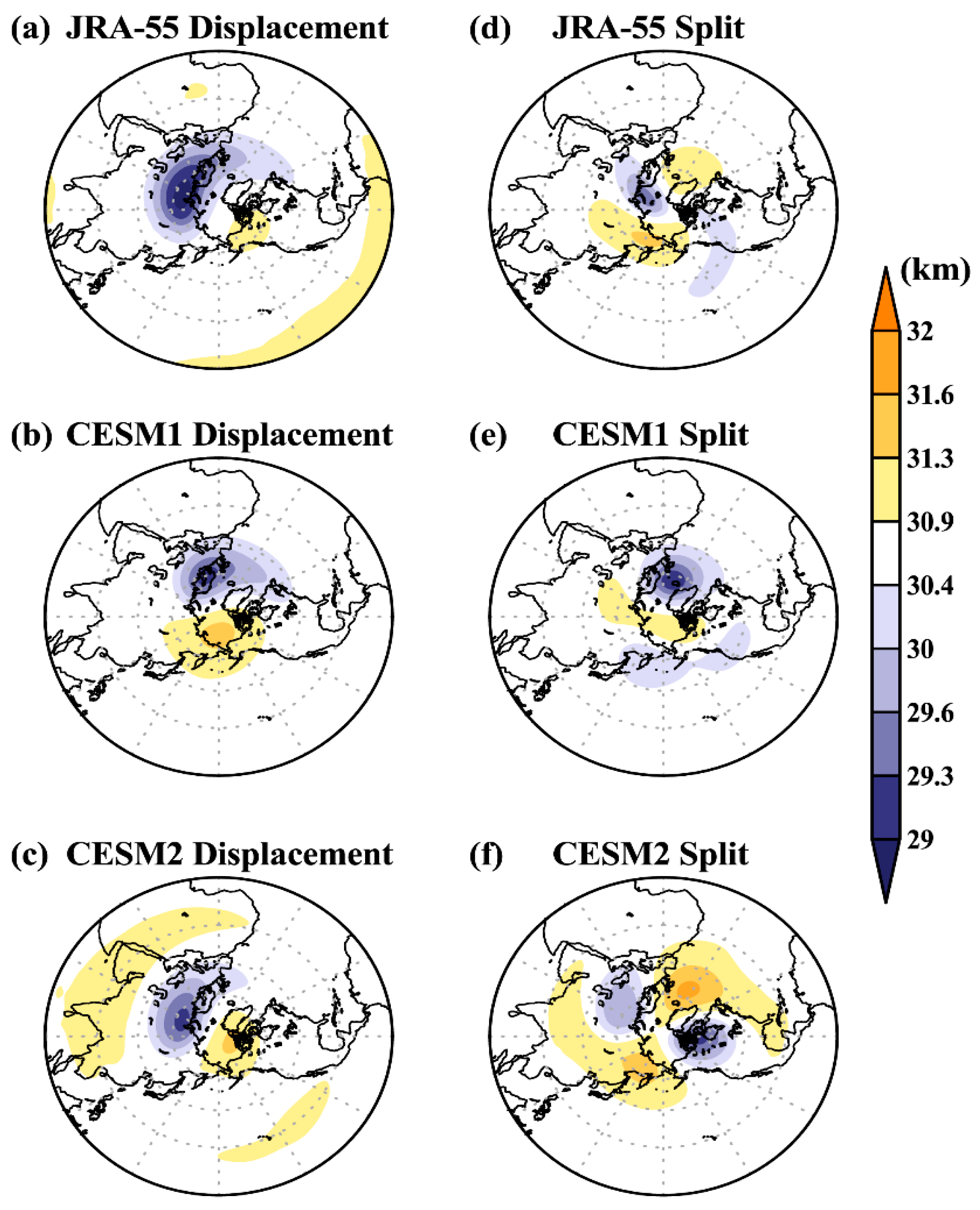
3.2. Evolution of the Stratospheric Circulation and Temperature during Vortex Displacement and Split SSWs

Three indicators, including the zonal wind in the circumpolar region (55–75° N), the polar temperature (60–90° N), and the polar geopotential height (60–90° N) area-averaged over the specified regions, are shown in this study to compare and evaluate the model performance of reproducing vortex displacement and split SSWs.
Figure 5 shows the composite pressure–time evolution for both types of SSWs from day −20 to day 60 relative to the SSW onset date for the JRA55 reanalysis, CESM1-WACCM, and CESM2-WACCM. It can be observed in Figure 5 that the composite evolution of the zonal mean zonal wind anomalies of vortex displacement SSWs is seemingly different from that of vortex split SSWs in observations. As the sample size becomes much larger, such difference in models between vortex displacement and split SSWs are much weaker than in JRA55. The westerly wind anomalies in both vortex displacement (Figure 5a) and split SSWs (Figure 5d) from the reanalysis rapidly weaken and reverse to the easterly wind anomalies in the stratosphere. Shortly after the SSW onset, the easterly anomalies reach the maximum (30 m/s) at 10 hPa, which is successfully reproduced by CESM1-WACCM (Figure 5b,e) and CESM2-WACCM (Figure 5c,f). The negative easterly anomalies stronger than 5 m/s can persist for more than a month in both types of SSWs in JRA55, which is well simulated in both models (Figure 5a–f). Comparing vortex displacement and split SSWs in JRA55, the latter on average is stronger than the former (Figure 5a,d,g). The different composite intensities between vortex displacement and split SSWs observed in JRA55 are also captured in CESM1-WACCM and CESM2-WACCM (Figure 5h,i), although such difference is less in CESM2-WACCM than in CESM1-WACCM. It might be concluded that vortex split SSWs have a stronger impact on the troposphere in previous studies [13,17]. However, if we see the left two columns in Figure 5, we can find that the easterly wind anomalies can descend to lower troposphere and near surface for both displacement and split SSWs in all datasets after the SSW onsets. The composite difference between vortex split and displacement SSWs is statistically significant in a long-term range after the SSW onset in JRA55 (Figure 5g), and split minus displacement SSW difference in CESM1-WACCM (Figure 5h) highly resembles the reanalysis. However, such difference is much smaller and less significant in CESM2-WACCM (Figure 5i). In addition, the negative wind anomalies descend down to the near surface more rapidly for vortex split SSWs than for displacement SSWs in all datasets [13,17].
The direction reversal of zonal wind is related to the increase of polar geopotential height by the geostrophic wind principle. Figure 6 shows the composite evolution of the polar height anomalies, which are consistent with the evolution of zonal wind anomalies (Figure 4) around the onset date. The positive height anomalies in both vortex displacement and split SSWs start to appear several days before the SSW onset date, consistent with the deceleration of circumpolar westerlies in Figure 5. The polar height anomalies reach maxima soon after the SSW onset in JRA55, which are also well resolved by models (Figure 6a–f). All the three datasets show that the positive height anomalies begin to decrease two weeks after the SSW onset and reverse to weak and nonsignificant negative height anomalies another two weeks later. However, because SSWs mainly appear in late winter and late-winter SSWs are usually weaker than midwinter events (Figure 4), it is shown once again that CESM2-WACCM somewhat underestimates the maximum polar height anomalies just after the SSW onset (Figure 6c,f). It can be observed once again that, in the reanalysis, the polar height anomalies for vortex split SSWs develop deeper in the troposphere and reach the near-surface sooner than the counterpart anomalies for vortex displacement SSWs. The reanalysis and models consistently show that the positive height anomalies for both vortex displacement and split SSWs propagate downward, but the near surface height anomalies for polar vortex split SSWs are larger than those for displacement SSWs. The positive height anomalies in the Arctic stratosphere within two weeks after the SSW onset are also consistently stronger for vortex split SSWs than for displacement events in the three datasets (Figure 6g–i).
The sharp rise of the polar temperature is also an important feature for SSWs [2,4,44] so the composite evolutions of the polar temperature anomalies are shown in Figure 7. The warming anomalies in observations first develop in the upper stratosphere, reach maxima (16 K) at the onset date, and propagate to the middle troposphere (Figure 7a–f). It should be noted that the warm temperature anomalies cannot reach the near surface but are coupled with the cold temperature anomalies in the lower troposphere. Namely, warm temperature anomalies in the Arctic stratosphere during SSWs corresponds to cold air outbreak in the lower troposphere. It can be seen that the near-surface air temperature after the SSW onset is colder and more significant for vortex split SSWs than displacement SSWs in JRA55 and CESM1-WACCM (top two rows in Figure 7): The minimum near-surface temperature anomalies can reach −1 K and −0.5 K for vortex split and displacement SSWs after the onset, respectively. In contrast, the near-surface air temperature anomalies show nonsignificant differences in CESM2-WACCM (Figure 7c,f,i). Such different surface responses to vortex displacement and split SSWs in JRA55 and CESM1-WACCM might reflect their different intensities. The intensities of the two types of SSWs are significantly different in JRA55 and CESM1-WACCM (Figure 5g,h, Figure 6g,h, and Figure 7g,h), whereas the intensities of the two types of SSWs in CESM2-WACCM are similar and their differences are nonsignificant at the 95% confidence level (Figure 5i, Figure 6i and Figure 7i).

3.3. Evolution of Tropospheric Circulation during Vortex Displacement and Split SSWs

It has been reported that the upward propagation of planetary waves originating in the troposphere can influence the stratospheric circulation and may induce SSW events [4,6,19,21], although some studies [64] declare that the tropospheric wave forcing may only affect about 30% of SSWs. In order to comprehend and evaluate the tropospheric circulation during different SSW stages, which may act as a trigger, Figure 8 and Figure 9 show the evolutions of extratropical geopotential height anomalies at 500 hPa for both types of SSWs, respectively.
The negative height anomalies centered over North Pacific from day −25 to day −15 and the positive height anomalies over Arctic Canada for both vortex displacement and split SSWs in the reanalysis (Figure 8a1 and Figure 9a1) resembles a positive PNA pattern and a negative WP pattern, which intensify planetary wave activity by interfering with the climatological trough and ridge [11,24,58]. The negative height anomalies over the North Pacific, east of US and the positive anomalies over Canada for vortex displacement SSWs are more persistent than for vortex split SSWs during 5–15 days before the SSW onset (Figure 8a2 and Figure 9a2), therefore the positive PNA for vortex displacement SSWs may be stronger than for split SSWs, which can project onto the wavenumber-1. In contrast, there is a second anomaly low center in west Europe for split SSWs, which together with the Pacific low center, project onto the wavenumber-2. Those differences between vortex displacement and split SSWs imply that wavenumber-1 is enhanced before the displacement SSW events and that wavenumber-2 is enhanced before vortex split SSWs [6,15,20,21]. The PNA and WP patterns largely weaken during the SSW onset (Figure 8a3 and Figure 9a3), and positive height anomalies appear over the high-latitude of the North Atlantic for vortex split SSWs, which project onto a negative NAO pattern (Figure 9a3) while the negative NAO-like response is not formed for displacement SSWs (Figure 9a3). It may imply that the impacts of vortex displacement and split SSWs on the troposphere, especially over the North Atlantic region, are different, consistent with previous studies [13,17]. It is noted that some uncertainties still exist due to the small sample size [18]. However, negative height anomalies form over Eurasia following the SSW onset for both vortex displacement and split SSWs (Figure 8a4,a5 and Figure 9a4,a5).
Generally, the positive PNA-like and negative WP-like pattern, as well as the negative height anomalies over the North Pacific before the SSW onset date, are successfully reproduced by both models (Figure 8b1,b2,c1,c2 and Figure 9b1,b2,c1,c2). The much stronger North Pacific low anomaly response than the North Atlantic low anomaly center mainly projects onto an enhanced wavenumber-1 in models for vortex displacement SSWs (Figure 8b1–b3,c1–c3), consistent with the reanalysis (Figure 8a1–a3). In contrast, the comparable North Pacific low anomaly center and North Atlantic low anomaly center before and during the SSW onset mainly project onto an enhanced wavenumber-2 (Figure 9a1–a3,b1–b3,c1–c3), which is well simulated in models. However, the negative NAO-like response in CESM2-WACCM during and after the SSW onset is much weaker for split SSWs than in CESM1-WACCM (Figure 9b,c).

3.4. Teleconnections and Upward Propagation of Planetary Waves from the Troposphere

It has been reported that extreme stratospheric events such as sudden stratospheric warmings are closely related to upward planetary waves from the extratropical troposphere [11,16,24,56,57,58], which can be revealed through teleconnections and the evolutions of eddy heat flux. For instance, studies have shown that SSWs may be triggered by negative WP and positive PNA patterns preceding SSWs. Furthermore, SSW events play an important role in regional weather anomalies such as negative NAO phase during SSW events, which is caused by downward propagation of the AO/NAM signals [2,9,19,65]. Additionally, studies have discussed whether there are significantly stronger positive AO/NAM anomalies near the surface following vortex splits [13,17,18]. Therefore, in order to evaluate the possible trigger preceding different types of SSWs and their difference in the surface impact, three teleconnections are calculated.
The evolutions of three teleconnections calculated from day −50 to day 50 with respect to the SSW onset date are displayed in Figure 10. The PNA for both types of SSWs stay mainly in its positive phase before the SSW onset date in observations, although it fluctuates frequently (Figure 10a,d). The WP index, however, develops in its negative phase before the SSW onset and reaches the minima simply several days before the SSW onset (Figure 10a,d). The NAO remains in its negative phase 20 days around the SSW onset for vortex displacement SSWs, while the NAO phase is mainly in its negative phase after the vortex split SSW onset. The negative NAO for vortex split SSWs appear stronger and more significant than that for vortex displacement SSWs. As in the reanalysis, both models also show that the negative WP occupies most of the period before SSW onset (Figure 10b,c,e,f), and the positive PNA is also simulated except that there is an abrupt drop of the PNA about a week before the vortex split SSW onset in CESM1-WACCM (Figure 10e).
The eddy heat flux ( v T ¯ ) is calculated because it can be used as a representation of the upward propagation of planetary waves (i.e., the vertical component of the Eliassen–Palm flux, Fz), which is almost proportional to the eddy heat flux [2,4,11,25,53]. Figure 11 and Figure 12 show the evolution of eddy heat flux from day −40 to day 40. It can be seen in both JRA55 and the models that large positive eddy heat flux anomalies suddenly turn negative after reaching maxima just several days before the SSW onset (Figure 11a–f). It is noticeable that the upward propagation for vortex displacement and split SSWs are different. Namely, the eddy heat flux anomalies for vortex split SSWs (Figure 11d) appear to be stronger than for vortex displacement SSWs (Figure 11a), which can also be further verified by the difference between vortex split and displacement SSWs (Figure 11g). In addition, the magnitude and duration difference between the two types of SSWs in observations can also be observed from the eddy heat flux at 10 hPa (Figure 12). The negative eddy heat flux after the SSW onset indicates that the upward propagation of planetary waves is suppressed by the easterlies when the downward impact becomes strong. However, both models do not show any significant difference of eddy heat flux between vortex displacement and split SSWs (Figure 11b,c,e,f). It can be concluded when the sample size becomes large, the difference in upward propagation of total waves might not be significantly large between vortex displacement and split SSWs.

3.5. Downward Impact of SSW

The evolution of the air temperature anomalies at 850 hPa in the Northern Hemisphere during different types of SSW events is shown in Figure 13 and Figure 14 to demonstrate their impacts on the lower troposphere and near surface. It is noticeable that there are no model data available at 850 hPa in Tibet Plateau, Greenland, and Rocky Mountains due to their high altitudes. The temperature anomaly patterns before SSW onset are in connection with the evolution of teleconnections while the temperature anomaly patterns afterward are also influenced by downward propagation of SSW-related signals.
It can be revealed from the reanalysis that large-scale cold anomalies occupy the North Eurasian continent before and during SSW onset while warm anomalies occur over the North American continent for vortex displacement SSWs (Figure 13a1–a3). This large-scale temperature pattern, however, is reversed after the polar vortex displacement SSW onset in JRA55: The North Eurasian continent is anomalously warm and the North American continent is anomalously cold (Figure 13a4,a5). The opposite land temperature patterns before and after the displacement SSWs are also identified in CESM1-WACCM and CESM2-WACCM (Figure 13b,c). Compared with JRA55, the cold temperature anomaly center in the Eurasian continent is further eastward biased before the vortex displacement SSW onset. The temperature patterns in Figure 12 are different from Figure 10 in Cao et al. [33]: They find that the northern Eurasian continent is anomalously cold all the way weeks before and after the SSW onset. Therefore, it is necessary to differentiate SSW types when we study the impact of the SSW events.
Consistent with Cao et al. [33], it is shown that before and during the split SSW onset, a cold northern Eurasian continent–warm North American continent pattern is observed, but both continents are dominated by cold air after the split SSW onset (Figure 14a). Therefore, the composite temperature pattern using all SSW events in Cao et al. [33] (see their Figure 10) is primarily dominated by vortex split SSWs (Figure 14a). The cold Eurasia–warm North America air temperature pattern before and during vortex split SSWs are well reproduced by CESM1-WACCM and CESM2-WACCM (Figure 14b,c). Similarly, the Eurasian and North American continents are almost covered with cold air temperature anomalies after the vortex split SSWs. In contrast, the temperature anomalies in CESM2-WACCM are much weaker than in CESM2-WACCM, especially during the post-SSW periods (Figure 14b,c), consistent with the relatively weaker SSW intensities in CESM2-WACCM.

4. Summary and Discussion

The reproducibility of vortex displacement and split SSW events in two versions of the CESM-WACCM coupled model during 1850–2005/2014 is evaluated in this study based on the JRA55 reanalysis during 1958–2015. A statistical and diagnostic analysis is conducted on the monthly and decadal distribution of two types of SSW events, their intensities, evolutions of the stratospheric and tropospheric circulation, and temperature. In particular, the tropospheric precursors for vortex displacement and split SSWs and their impacts on the near-surface temperature are discussed. The main concluding remarks in this paper are as follows.
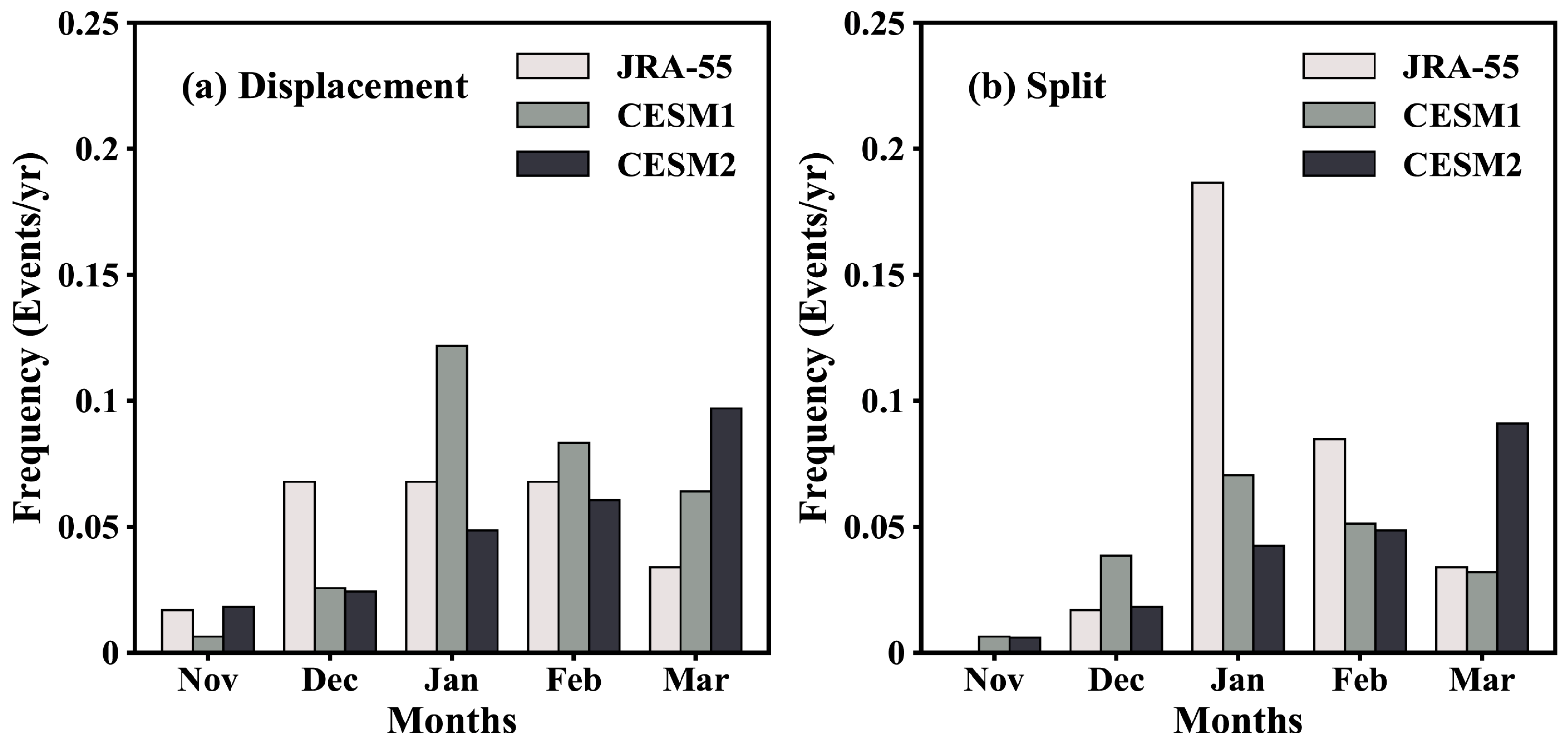
  • SSW events are searched and their displacement and split types are categorized using the WMO definition [43] and a threshold-based classification method by Seviour et al. [18], respectively. It is found that the ratio of vortex displacement to split SSWs is about 0.79 in the JRA55 reanalysis while the ratio is 1.2–1.4 in the CESM1-WACCM and CESM2-WACCM models, which means that the CESM-WACCM model family tends to simulate more vortex displacement SSWs than in the reanalysis. The seasonal distribution somewhat differs between two types of SSW events in observations. The frequency of both SSW types peaks in January. November is the wintertime month when least SSWs occur for both types. Although CESM2-WACCM is expected to improve over CESM1-WACCM, no statistical proof is found that the seasonal distributions of both SSW types are simulated better by CESM2-WACCM than CESSM1-WACCM.
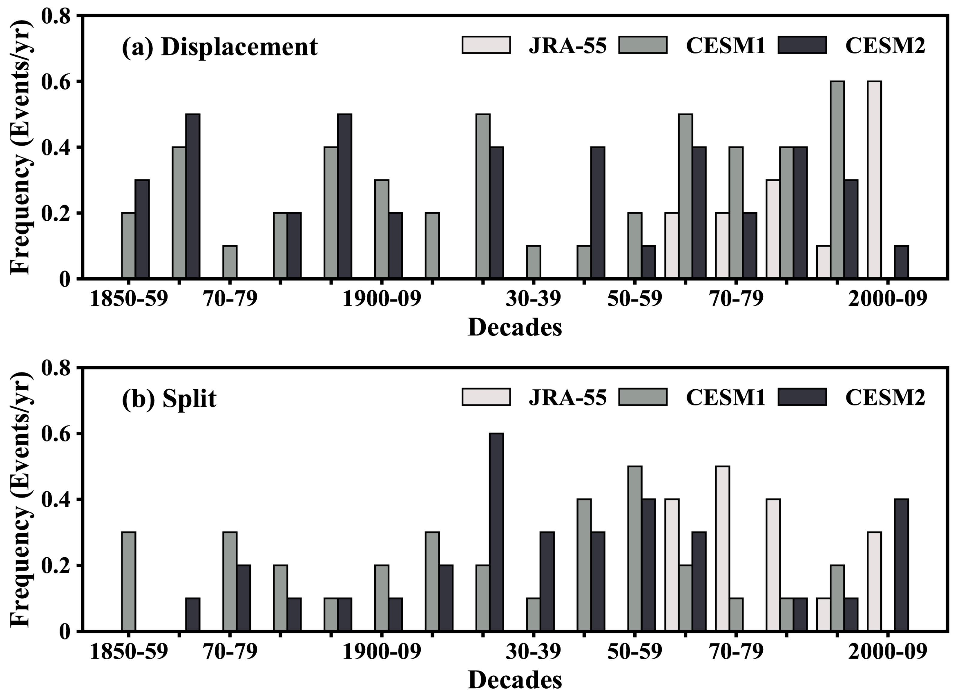
  • The decadal frequency of both types of SSW events changes quasi-periodically in both the reanalysis and the models, which may reflect the internal variability of the stratosphere. All datasets show that a low/high frequency of vortex split SSWs tends to be accompanied by a high/low frequency of vortex displacement SSWs. Due to the atmospheric chaos and the free run of the atmosphere-ocean system in historical experiments of both models, the numbers of SSW events in each decade are very different in model and the reanalysis.
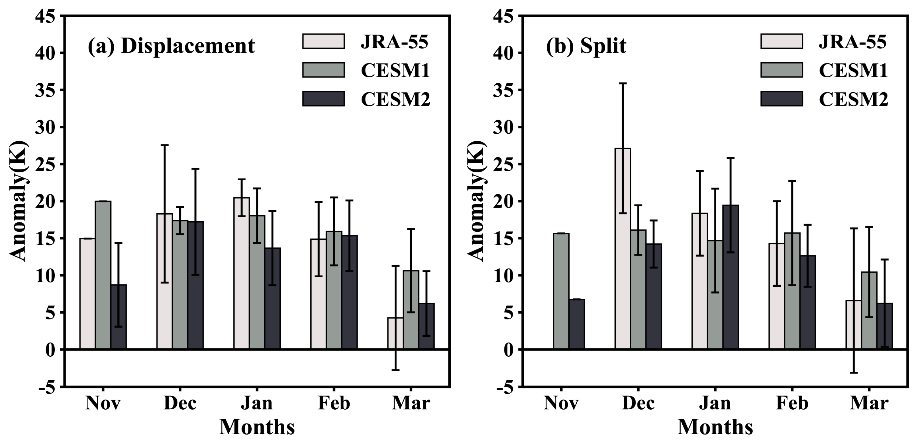
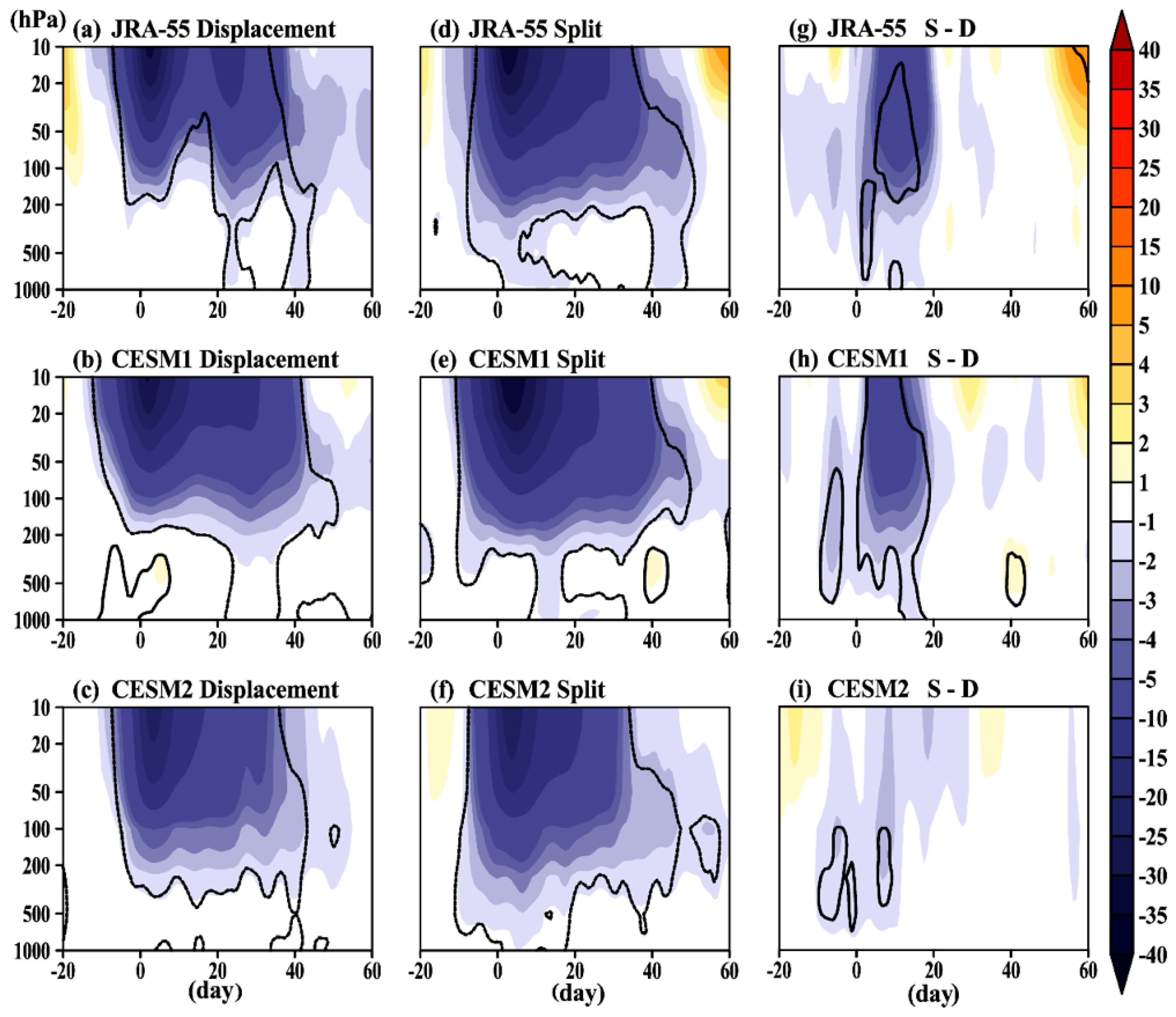
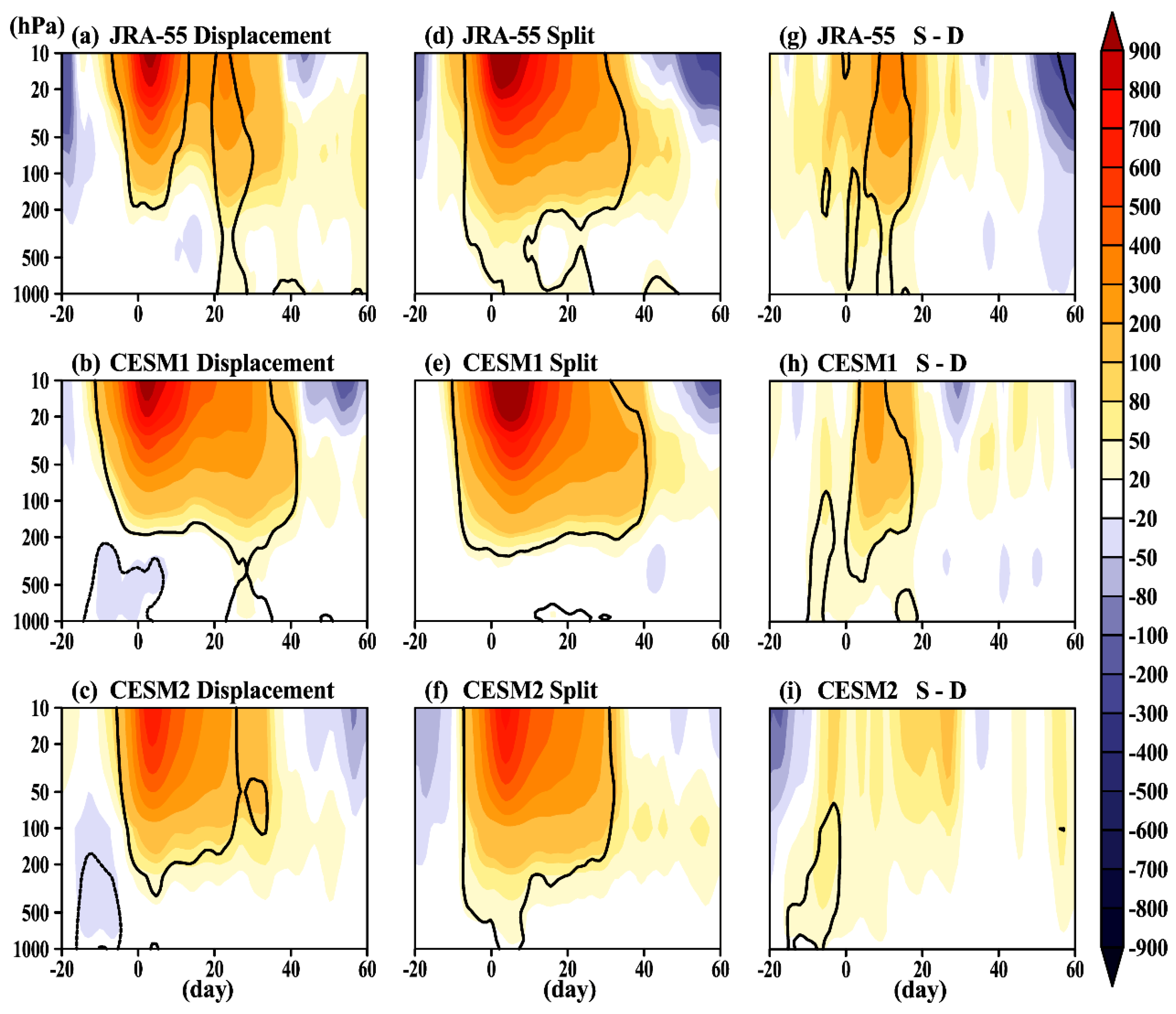
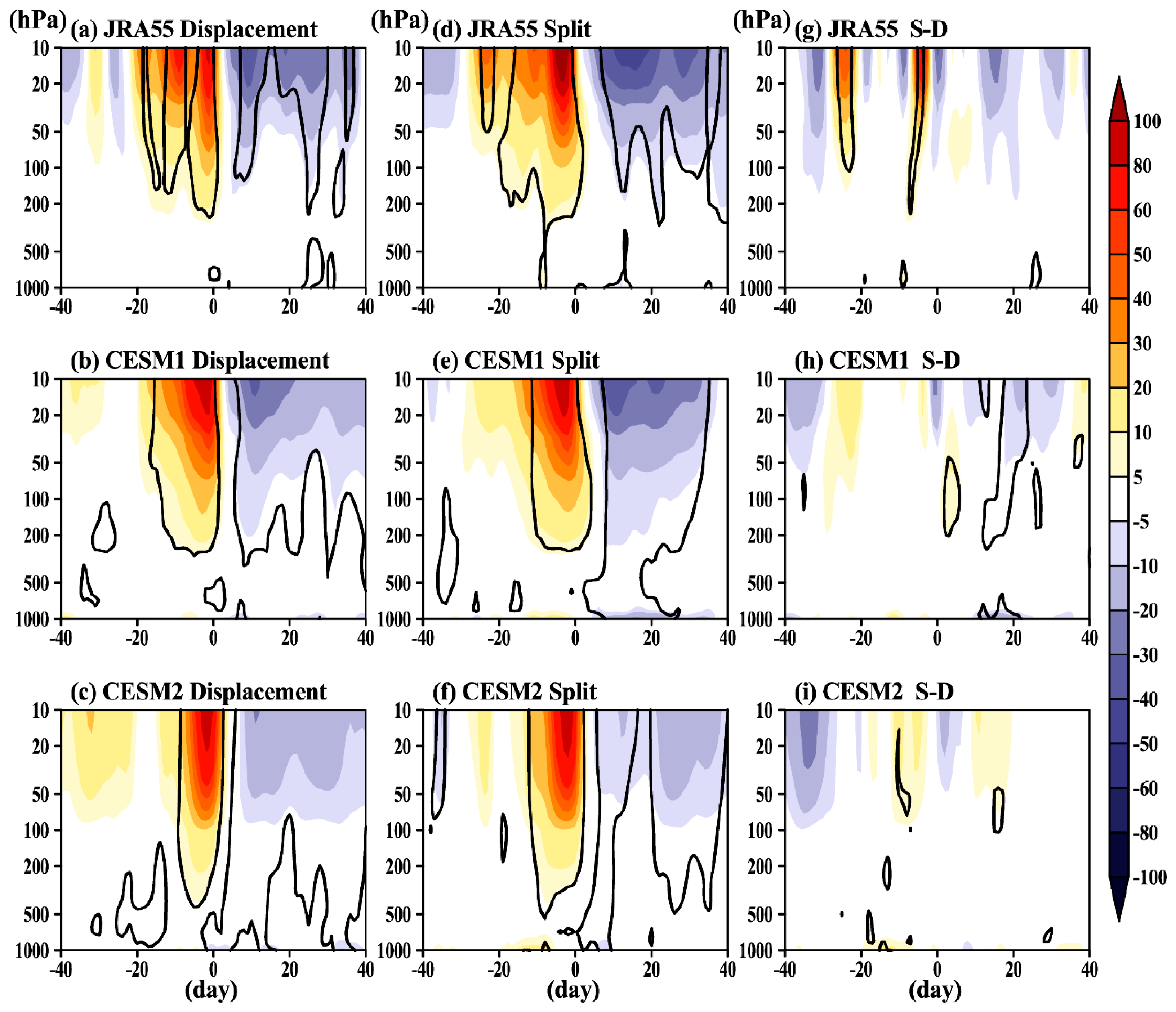
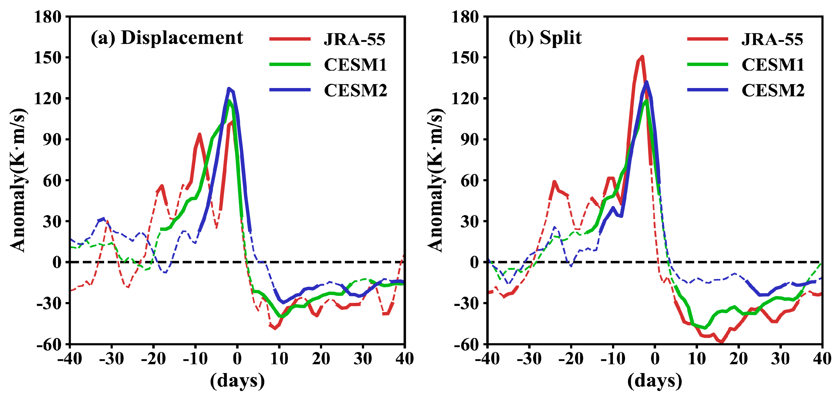
  • The polar temperature anomalies, height anomalies, wind anomalies, and eddy heat flux anomalies for vortex split SSWs are identified to be stronger and more persistent than those for vortex displacement SSWs in the reanalysis. In contrast, as the sample size becomes large in the models, and the differences between vortex displacement and split SSWs are smaller than in JRA55. The circulation and temperature anomalies in CESM1-WACCM more resemble JRA55 quantitatively, and the anomaly amplitudes in CESM2-WACCM are underestimated due to the worse phase locking of SSWs from CESM2-WACCM. Although the total eddy heat flux by all waves before vortex split SSWs are much stronger than displacement SSWs in JRA55, such differences between two types of SSWs in models are small.
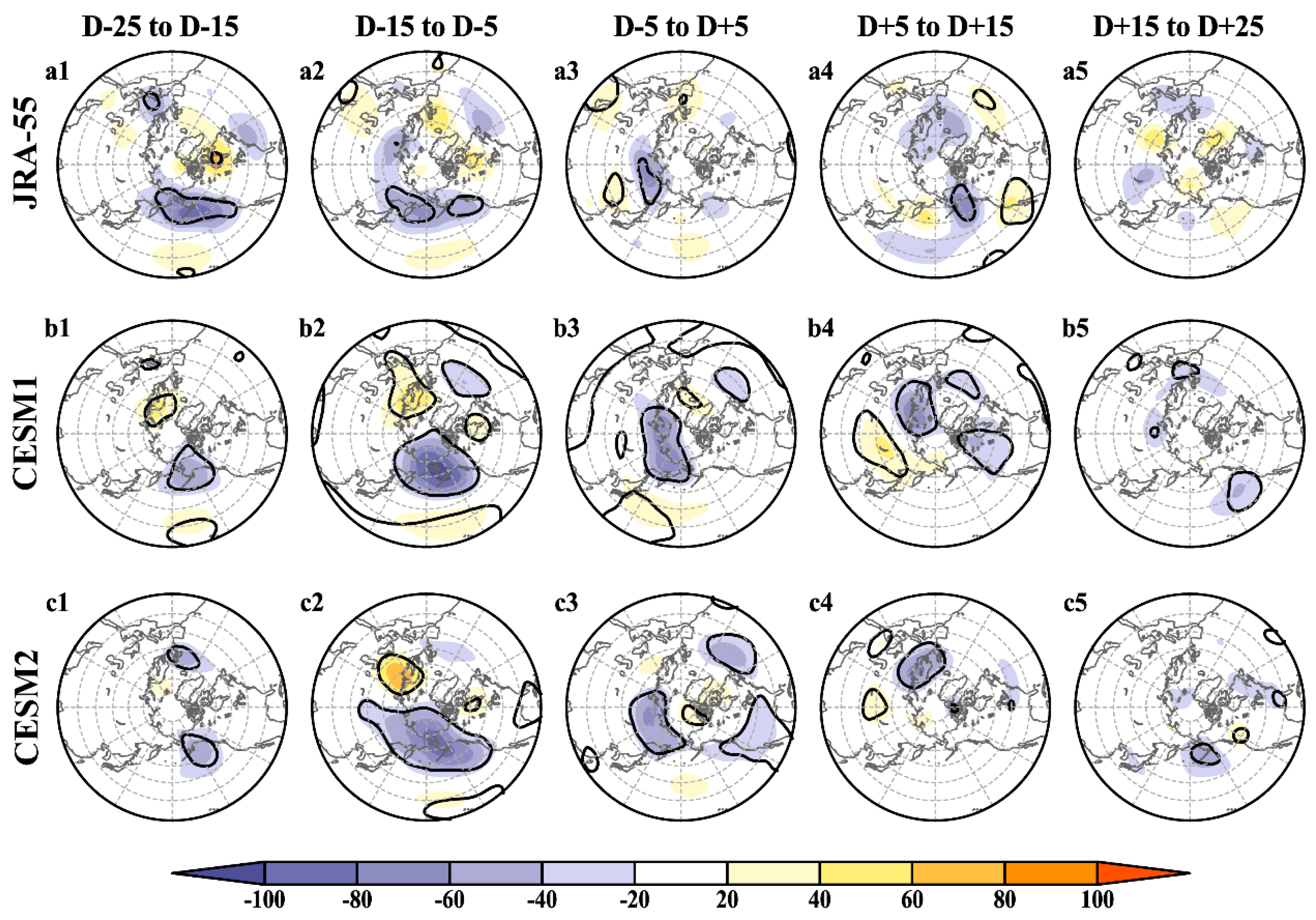
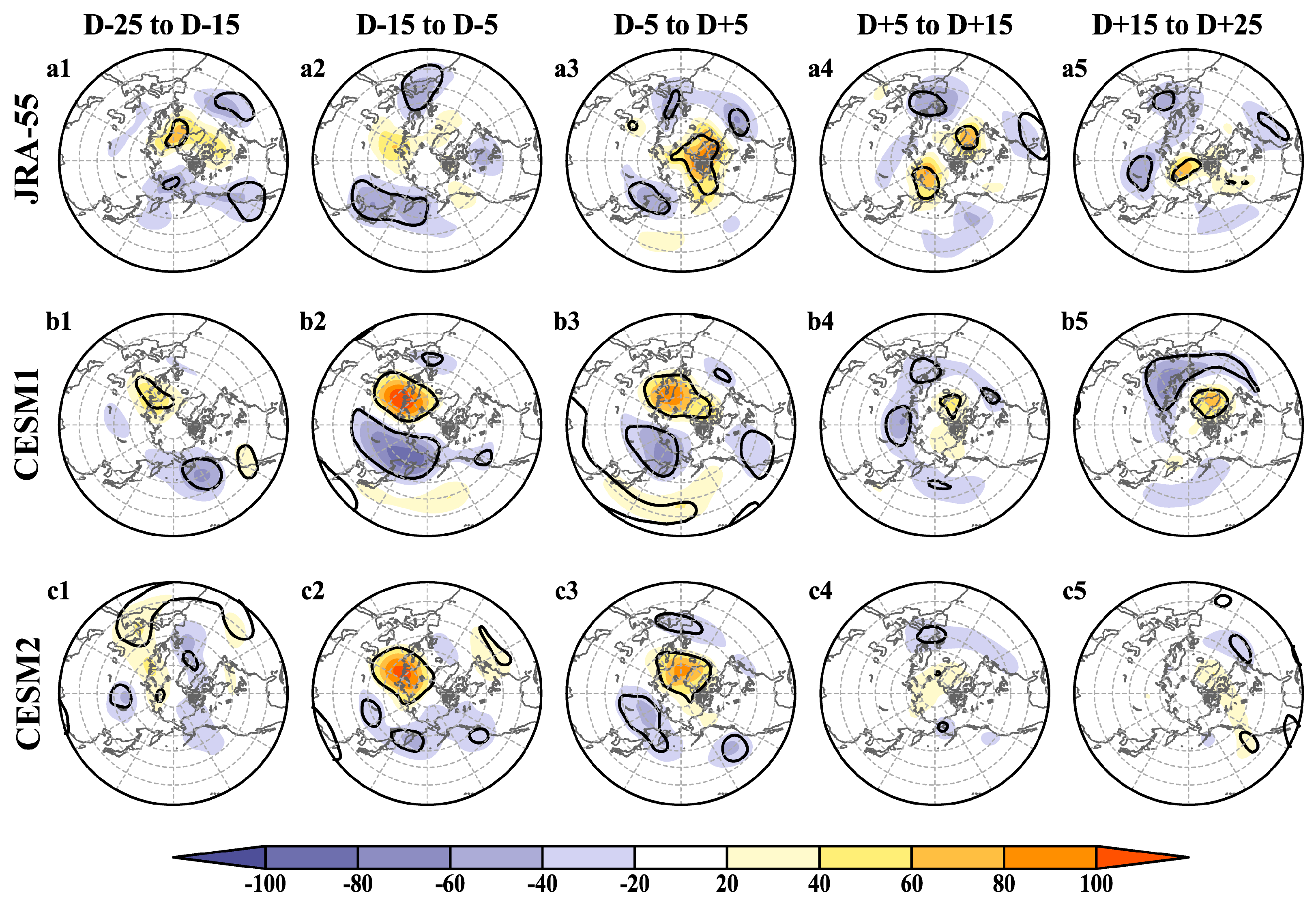
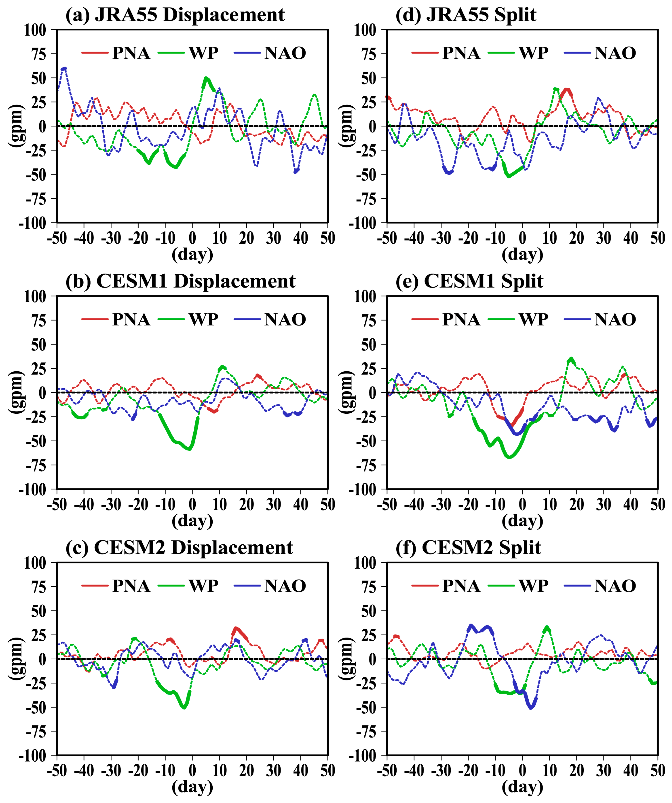
  • It is shown in both observations and the models that positive PNA and negative WP patterns in the troposphere precedes vortex displacement and split SSWs, which indicates the enhancement of upward planetary waves from the troposphere before SSW events. The North Pacific low anomaly center is much stronger than the North Atlantic counterpart before and during the displacement SSWs, which mainly projects onto an enhanced wavenumber-1. In contrast, the North Pacific and North Atlantic low anomaly centers before and during split SSWs are comparable, which corresponds to an enhanced wavenumber-2. In addition, as in JRA55, the models also show that negative NAO-like pattern after split SSW onset is stronger than that after displacement SSW onset.
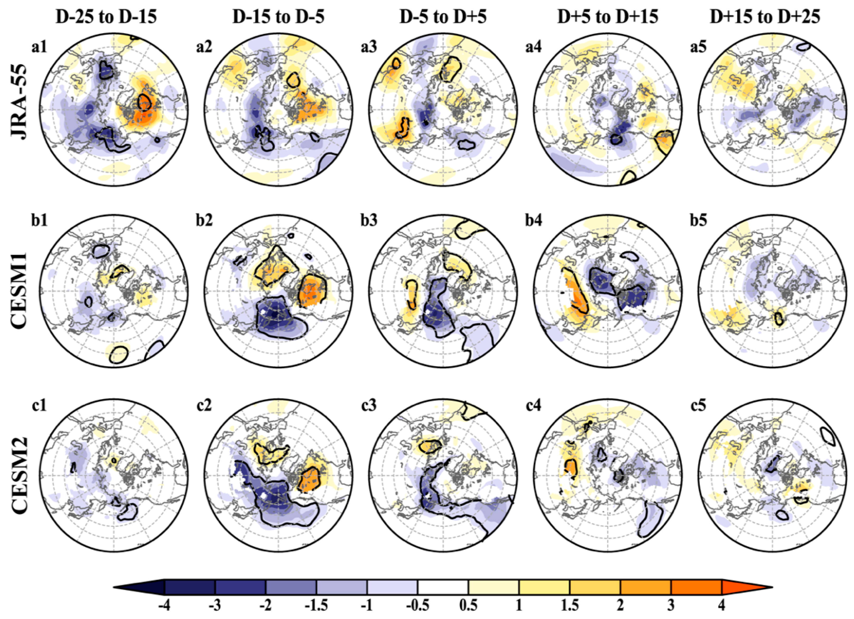
  • A cold Eurasian continent–warm North American continent pattern appears during some pre-SSW periods for both types of SSWs. On the contrary, a warm Eurasian continent–cold North American continent pattern appears after the displacement SSW onset. In contrast, both continents are anomalously cold after the split SSW onset. The near-surface air temperature patterns before and after the SSW onset are well reproduced by both models, although the temperature anomalies after the split SSW onset in CESM2-WACCM are somewhat underestimated.
The performance of the CESM1-WACCM and CESM2-WACCM models in simulating different types of SSW events are comprehensively assessed in this study. Although some improvements have been achieved for CESM2-WACCM when compared with CESM1-WACCM, new biases might be generated. For example, it has been noted that CESM1-WACCM cannot reproduce the QBO but CESM2-WACCM can spontaneously generate the QBO, which is a great improvement for the new CESM-WACCM version (a paper by Rao et al. 2019 submitted to Journal of Climate). However, new biases regarding SSWs also appear, including the seasonal shift of the SSWs to late winter in CESM1-WACCM, underestimation of the SSW intensity, and obscurity of the near-surface response to the two types of SSWs. It is still unknown how those biases are produced in CESM2-WACCM. In addition, more CMIP6 models have released their historical runs, and a more comprehensive comparison between CMIP5 and CMIP6 models in simulating SSWs is still lacking. However, the comparison between CESM1-WACCM and CESM2-WACCM still provides useful information for NCAR model developers and also corrects our conventional idea that a new model version is destined to behave better than the old version. The fact might not be so.

Author Contributions

Conceptualization, J.R. and S.-M.L.; methodology, Y.H.C. and C.C.; software, C.C. and Y.-H.C.; validation, J.R. and S.-M.L.; formal analysis, S.-M.L. and J.R.; investigation, Y.-H.C. and S.-Y.L.; writing—original draft preparation, S.-M.L. and S.-Y.L.; writing—review and editing, J.R.; visualization, M.-H.M. and Y.-B.W.; supervision, J.R.; project administration, S.-M.L. and C.C.

Funding

This work was jointly supported by grants from the National Natural Science Foundation of China (41705024), the National Key R&D Program of China (2016YFA0602104), and College Students’ Practice Innovation Training Program of Jiangsu Province (201810300009Z).

Acknowledgments

We acknowledge the Japanese Meteorological Agency for providing the JRA55 reanalysis data. The CESM1-WACCM and CESM2-WACCM historical runs were provided by CMIP and NCAR upon request.

Conflicts of Interest

The authors declare no conflict of interest.

References

  1. O’Neill, A.; Charlton-Perez, A.J.; Polvani, L.M. Stratospheric sudden warmings. In Encyclopedia of Atmospheric Science, 2nd ed.; North, G.R., Pyle, J., Zhang, F., Eds.; Elsevier: London, UK, 2014; Volume 4, pp. 30–40. [Google Scholar]
  2. Limpasuvan, V.; Thompson, D.W.J.; Hartmann, D.L. The life cycle of the Northern Hemisphere sudden stratospheric warmings. J. Clim. 2004, 17, 2584–2596. [Google Scholar] [CrossRef]
  3. Manney, G.L.; Krnney, G.; Sabutis, J.L.; Sena, S.A.; Pawson, S. The remarkable 2003–2004 winter and other recent warm winters in the Arctic stratosphere since the late 1990s. J. Geophys. Res. 2005, 110, 583–595. [Google Scholar] [CrossRef]
  4. Charlton, A.J.; Polvani, L.M. A new look at stratospheric sudden warmings. Part I: Climatology and modeling benchmarks. J. Clim. 2007, 20, 449–469. [Google Scholar] [CrossRef]
  5. Scherhag, R. Die explosionsartigen Stratospherenerwarmingen des Spatwinters, 1951–1952. Ber. Deut. Wetterd. (U.S. Zone) 1952, 6, 51–63. [Google Scholar]
  6. Matsuno, T. A dynamical model of the stratospheric sudden warming. J. Atmos. Sci. 1971, 28, 1479–1494. [Google Scholar] [CrossRef]
  7. McIntyre, M.E. How well do we understand the dynamics of stratospheric warming? J. Meteorol. Soc. Jpn. 1982, 60, 37–64. [Google Scholar] [CrossRef]
  8. Limpasuvan, V.; Hartmann, D.L. Eddies and the annular modes of climate variability. Geophys. Res. Lett. 1999, 26, 3133–3136. [Google Scholar] [CrossRef] [Green Version]
  9. Black, R.X. Stratospheric forcing of surface climate in the Arctic Oscillation. J. Clim. 2002, 15, 268–277. [Google Scholar] [CrossRef]
  10. Kim, Y.J.; Flatau, M. Hindcasting the January 2009 Arctic sudden stratospheric warming and its influence on the Arctic Oscillation with unified parameterization of orographic drag in NOGAPS. Part I: Extended-range stand-alone forecast. Weather Forecast. 2010, 25, 1628–1644. [Google Scholar] [CrossRef]
  11. Rao, J.; Ren, R.; Chen, H.; Yu, Y.; Zhou, Y. The stratospheric sudden warming event in February 2018 and its prediction by a climate system model. J. Geophys. Res. Atmos. 2018, 123, 13332–13345. [Google Scholar] [CrossRef]
  12. Mukougawa, H.; Sakai, H.; Hirooka, T. High sensitivity to the initial condition for the prediction of stratospheric sudden warming. Geophys. Res. Lett. 2005, 32, L08814. [Google Scholar] [CrossRef]
  13. Mitchell, D.M.; Gray, L.J.; Anstey, J.; Baldwin, M.P.; Charlton-Perez, A.J. The Influence of Stratospheric Vortex Displacements and Splits on Surface Climate. J. Clim. 2013, 26, 2668–2682. [Google Scholar] [CrossRef] [Green Version]
  14. Seviour, W.J.M.; Mitchell, D.M.; Gray, L.J. A practical method to identify displaced and split stratospheric polar vortex events. Geophys. Res. Lett. 2013, 40, 5268–5273. [Google Scholar] [CrossRef] [Green Version]
  15. Nakagawa, K.I.; Yamazaki, K. What kind of stratospheric sudden warming propagates to the troposphere? Geophys. Res. Lett. 2006, 33, L04801. [Google Scholar] [CrossRef]
  16. Maycock, A.C.; Hitchcock, P. Do split and displacement sudden stratospheric warmings have different annular mode signatures? Geophys. Res. Lett. 2015, 42, 10943–10951. [Google Scholar] [CrossRef]
  17. O’Callaghan, A.; Joshi, M.; Stevens, D.; Mitchell, D. The effects of different sudden stratospheric warming types on the ocean. Geophys. Res. Lett. 2014, 41, 7739–7745. [Google Scholar] [CrossRef] [Green Version]
  18. Seviour, W.J.M.; Gray, L.J.; Mitchell, D.M. Stratospheric polar vortex splits and displacements in the high-top CMIP5 climate models. J. Geophys. Res. 2016, 121, 1400–1413. [Google Scholar] [CrossRef] [Green Version]
  19. Rao, J.; Ren, R.; Chen, H.; Liu, X.; Yu, Y.; Yang, Y. Sub-seasonal to seasonal hindcasts of stratospheric sudden warming by BCC_CSM1.1(m): A comparison with ECMWF. Adv. Atmos. Sci. 2019, 35, 479–494. [Google Scholar] [CrossRef]
  20. Rao, J.; Ren, R. Varying stratospheric responses to tropical Atlantic SST forcing from early to late winter. Clim. Dyn. 2018, 51, 2079–2096. [Google Scholar] [CrossRef]
  21. Yoden, S.; Yamaga, T.; Pawson, S.; Langematz, U. A composite analysis of the stratospheric sudden warmings simulated in a perpetual January integration of the Berlin TSM GCM. J. Meteorol. Soc. Japan 1999, 77, 431–445. [Google Scholar] [CrossRef]
  22. Holton, J.R.; Tan, H.C. The Influence of the equatorial quasi-biennial oscillation on the global circulation at 50mb. J. Atmos. Sci. 1980, 37, 2200–2208. [Google Scholar] [CrossRef]
  23. Naito, Y.; Taguchi, M.; Yoden, S. A parameter sweep experiment on the effects of the equatorial QBO on stratospheric sudden warming events. J. Atmos. Sci. 2003, 60, 1380–1394. [Google Scholar] [CrossRef]
  24. Garfinkel, C.I.; Hartmann, D.L. Effects of the El Niño–Southern oscillation and the quasi-biennial oscillation on polar temperatures in the stratosphere. J. Geophys. Res. 2007, 112, D19112. [Google Scholar] [CrossRef]
  25. Rao, J.; Ren, R. Parallel comparison of the 1982/83, 1997/98 and 2015/16 super El Niños and their effects on the extratropical stratosphere. Adv. Atmos. Sci. 2017, 34, 1121–1133. [Google Scholar] [CrossRef]
  26. Taguchi, M. Predictability of major stratospheric sudden warmings: Analysis results from JMA operational 1-month ensemble predictions from 2001/02 to 2012/13. J. Atmos. Sci. 2016, 73, 789–806. [Google Scholar] [CrossRef]
  27. Peters, D.H.W.; Schneidereit, A.; Bügelmayer, M.; Zülicke, C.; Kirchner, I. Atmospheric circulation changes in response to an observed stratospheric zonal ozone anomaly. Atmos.-Ocean 2014, 53, 74–88. [Google Scholar] [CrossRef]
  28. Rao, J.; Yu, Y.; Guo, D.; Shi, C.; Chen, D.; Hu, D. Evaluating the Brewer–Dobson circulation and its responses to ENSO, QBO, and the solar cycle in different reanalyses. Earth Planet. Phys. 2019, 3, 166–181. [Google Scholar] [CrossRef]
  29. Cohen, J.; Jones, J. Tropospheric precursors and stratospheric warmings. J. Clim. 2011, 24, 1780–1790. [Google Scholar] [CrossRef]
  30. Hitchcock, P.; Simpson, I. The downward influence of sudden stratospheric warmings. J. Atmos. Sci. 2014, 71, 3856–3876. [Google Scholar] [CrossRef]
  31. Rao, J.; Ren, R.C.; Chen, H.; Liu, X.; Yu, Y.; Hu, J.; Zhou, Y. Predictability of stratospheric sudden warmings in the Beijing Climate Center forecast system with statistical error corrections. J. Geophys. Res. Atmos. 2019, 124, 8385–8400. [Google Scholar] [CrossRef]
  32. Taguchi, M. Comparison of subseasonal-to-seasonal model forecasts for major stratospheric sudden warmings. J. Geophys. Res. Atmos. 2018, 123, 10231–210247. [Google Scholar] [CrossRef]
  33. Cao, C.; Chen, Y.H.; Rao, J.; Liu, S.M.; Li, S.Y.; Ma, M.H.; Wang, Y.B. Statistical characteristics of major sudden stratospheric warming events in CESM1-WACCM: A comparison with the JRA55 and NCEP/NCAR reanalyses. Atmosphere 2019, 10, 519. [Google Scholar] [CrossRef]
  34. Marsh, D.R.; Mills, M.J.; Kinnison, D.E.; Lamarque, J.F.; Calvo, N.; Polvani, L.M. Climate change from 1850 to 2005 simulated in CESM1(WACCM). J. Clim. 2013, 26, 7372–7391. [Google Scholar] [CrossRef]
  35. Ren, R.C.; Rao, J.; Wu, G.X.; Cai, M. Tracking the delayed response of the northern winter stratosphere to ENSO using multi reanalyses and model simulations. Clim. Dyn. 2017, 48, 2859–2879. [Google Scholar] [CrossRef]
  36. Richter, J.H.; Sassi, F.; Garcia, R.R. Toward a physically based gravity wave source parameterization in a general circulation model. J. Atmos. Sci. 2010, 67, 136–156. [Google Scholar] [CrossRef]
  37. Gettelman, A.; Hannay, C.; Bacmeister, J.T.; Neale, R.B.; Pendergrass, A.G.; Danabasoglu, G.; Lamarque, J.F.; Fasullo, J.T.; Bailey, D.A.; Lawrence, D.M.; et al. High climate sensitivity in the Community Earth System Model Version 2 (CESM2). Geophys. Res. Lett. 2019, 46, 8329–8337. [Google Scholar] [CrossRef]
  38. Knutti, R.; Masson, D.; Gettelman, A. Climate model genealogy: Generation CMIP5 and how we got there. Geophys. Res. Lett. 2013, 40, 1194–1199. [Google Scholar] [CrossRef]
  39. Martineau, P.; Son, S.-W.; Taguchi, M.; Butler, A.H. A comparison of the momentum budget in reanalysis datasets during sudden stratospheric warming events. Atmos. Chem. Phys. 2018, 18, 7169–7187. [Google Scholar] [CrossRef] [Green Version]
  40. Gerber, E.P.; Martineau, P. Quantifying the variability of the annular modes: Reanalysis uncertainty vs. sampling uncertainty. Atmos. Chem. Phys. 2018, 18, 17099–17117. [Google Scholar] [CrossRef]
  41. Rao, J.; Ren, R.; Xia, X.; Shi, C.; Guo, D. Combined impact of El Niño–Southern Oscillation and Pacific Decadal Oscillation on the northern winter stratosphere. Atmosphere 2019, 10, 211. [Google Scholar] [CrossRef]
  42. Kobayashi, S.; Ota, Y.; Harada, Y.; Ebita, A.; Moriya, M.; Onoda, H.; Onogi, K.; Kamahori, H.; Kobayashi, C.; Endo, H.; et al. The JRA-55 reanalysis: General specifications and basic characteristics. J. Meteorol. Soc. Japan 2015, 93, 5–48. [Google Scholar] [CrossRef]
  43. Andrews, D.G.; Holton, J.R.; Leovy, C.B. Middle Atmosphere Dynamics; Academic Press: Cambridge, MA, USA, 1985; p. 489. [Google Scholar]
  44. Butler, A.H.; Seidel, D.J.; Hardiman, S.C.; Butchart, N.; Birner, T.; Match, A. Defining sudden stratospheric warmings. Bull. Am. Meteorol. Soc. 2015, 96, 1913–1928. [Google Scholar] [CrossRef]
  45. Korenkov, Y.N.; Klimenko, V.V.; Klimenko, M.V.; Bessarab, F.S.; Korenkova, N.A.; Ratovsky, K.G.; Chernigovskaya, M.A.; Shcherbakov, A.A.; Sahai, Y.; Fagundes, P.R.; et al. The global thermospheric and ionospheric response to the 2008 minor sudden stratospheric warming event. J. Geophys. Res. Space Phys. 2012, 117, A10309. [Google Scholar] [CrossRef]
  46. Thiéblemont, R.; Ayarzagüena, B.; Matthes, K.; Bekki, S.; Abalichin, J.; Langematz, U. Drivers and surface signal of interannual variability of boreal stratospheric final warmings. J. Geophys. Res. Atmos. 2019, 124, 5400–5417. [Google Scholar] [CrossRef]
  47. Mitchell, D.M.; Charlton-Perez, A.J.; Gray, L.J. Characterizing the variability and extremes of the stratospheric polar vortices using 2D moment analysis. J. Atmos. Sci. 2011, 68, 1194–1213. [Google Scholar] [CrossRef]
  48. Mitchell, D.M.; Charlton-Perez, A.J.; Gray, L.J. The structure and evolution of the stratospheric vortex in response to natural forcings. J. Geophys. Res. 2011, 116, D15110. [Google Scholar] [CrossRef]
  49. Waugh, D.W. Elliptical diagnostics of stratospheric polar vortices. Q. J. R. Meteorol. Soc. 1997, 123, 1725–1748. [Google Scholar] [CrossRef]
  50. Waugh, D.W.; Randel, W.J. Climatology of arctic and antarctic polar vortices using elliptical diagnostics. J. Atmos. Sci. 1999, 56, 1594–1613. [Google Scholar] [CrossRef]
  51. Matthewman, N.J.; Esler, J.G.; Charlton-Perez, A.J.; Polvani, L.M. A new look at stratospheric sudden warmings. Part III: Polar vortex evolution and vertical structure. J. Clim. 2009, 22, 1566–1585. [Google Scholar] [CrossRef]
  52. Polvani, L.M.; Sun, L.; Butler, A.H.; Richter, J.H.; Deser, C. Distinguishing stratospheric sudden warmings from ENSO as key drivers of wintertime climate variability over the North Atlantic and Eurasia. J. Clim. 2017, 30, 1959–1969. [Google Scholar] [CrossRef]
  53. Rao, J.; Ren, R. A decomposition of ENSO’s impacts on the northern winter stratosphere: Competing effect of SST forcing in the tropical Indian Ocean. Clim. Dyn. 2016, 46, 3689–3707. [Google Scholar] [CrossRef]
  54. Dai, Y.; Tan, B.K. The western Pacific pattern precursor of major stratospheric sudden warmings and the ENSO modulation. Environ. Res. Lett. 2016, 11, 124032. [Google Scholar] [CrossRef] [Green Version]
  55. Hu, J.G.; Li, T.; Xu, H.M.; Yang, S.Y. Lessened response of boreal winter stratospheric polar vortex to El Niño in recent decades. Clim. Dyn. 2017, 49, 263–278. [Google Scholar] [CrossRef]
  56. Garfinkel, C.I.; Benedict, J.J.; Maloney, E.D. Impact of the MJO on the boreal winter extratropical circulation. Geophys. Res. Lett. 2014, 41, 6055–6062. [Google Scholar] [CrossRef]
  57. Rao, J.; Ren, R.C. Asymmetry and nonlinearity of the influence of ENSO on the northern winter stratosphere: 1. Observations. J. Geophys. Res. 2016, 121, 9000–9016. [Google Scholar] [CrossRef] [Green Version]
  58. Rao, J.; Ren, R.C. Asymmetry and nonlinearity of the influence of ENSO on the northern winter stratosphere: 2. Model study with WACCM. J. Geophys. Res. 2016, 121, 9017–9032. [Google Scholar] [CrossRef]
  59. Wallace, J.M.; Gutzler, D.S. Teleconnections in the geopotential height field during the northern hemisphere winter. Mon. Weather Rev. 1981, 109, 784–812. [Google Scholar] [CrossRef]
  60. Hu, J.G.; Ren, R.C.; Xu, H.M. Occurrence of winter stratospheric sudden warming events and the seasonal timing of spring stratospheric final warming. J. Atmos. Sci. 2014, 71, 2319–2334. [Google Scholar] [CrossRef]
  61. Butler, A.H.; Sjoberg, J.P.; Seidel, D.J.; Rosenlof, K.H. A sudden stratospheric warming compendium. Earth Sys. Sci. Data 2017, 9, 63–76. [Google Scholar] [CrossRef] [Green Version]
  62. Wang, H.Z.; Rao, J.; Sheng, C.; Wang, B. Statistical characteristics of the Northern Hemisphere stratospheric sudden warming and its seasonality (1948–2015). Tran. Atmos. Sci. 2019, 42. (In Chinese) [Google Scholar] [CrossRef]
  63. Rao, J.; Ren, R.C.; Yang, Y. Parallel comparison of the northern winter stratospheric circulation in reanalysis and in CMIP5 models. Adv. Atmos. Sci. 2015, 32, 952–966. [Google Scholar] [CrossRef]
  64. de la Cámara, A.; Birner, T.; Albers, J.R. Are sudden stratospheric warmings preceded by anomalous tropospheric wave activity? J. Clim. 2019. [Google Scholar] [CrossRef]
  65. Baldwin, M.P.; Dunkerton, T.J. Stratospheric harbingers of anomalous weather regimes. Science 2001, 294, 581–584. [Google Scholar] [CrossRef] [PubMed]
Figure 1. Polar projection of the geopotential heights (units: km) at 10 hPa in (a,d) the Japanese Meteorological Agency 55-year Reanalysis (JRA55), (b,e) community Earth system model version 1–the whole atmosphere community climate model (CESM1-WACCM), and (c,f) CESM2-WACCM during vortex displacement sudden stratospheric warmings (SSWs) on (a) 30 November 1968, (b) 6 January 1880, (c) 26 February 1854 and vortex split SSWs on (d) 2 January 1963, (e) 20 January 2005, (f) 24 February 1902.
Atmosphere 10 00679 g001
Figure 2. The frequency distribution (units: Events/year) of (a) vortex displacement SSWs and (b) vortex split SSWs in each wintertime month in the JRA55 reanalysis (light grey) during 1958–2015, CESM1-WACCM (dark grey), and CESM2-WACCM (black) during 1850–2005/2014.
Atmosphere 10 00679 g002
Figure 3. The frequency distribution (units: Events/year) of (a) vortex displacement SSWs and (b) vortex split SSWs in each decade in the JRA55 reanalysis from the 1960s to the 2000s (light grey) and in CESM1-WACCM (dark grey), and CESM2-WACCM (black) from the 1850s to the 2000s/2010s.
Atmosphere 10 00679 g003
Figure 4. Composite area-weighted polar (60°–90° N) temperature anomaly (units: K) at 10 hPa, ±5 days from the onset date of (a) vortex displacement SSWs and (b) vortex split SSWs in each wintertime month for the JRA55 reanalysis (light grey) during 1958–2015, CESM1-WACCM (dark grey), and CESM2-WACCM (black) during 1850–2005/2014. The error bar denotes the inter-case standard deviation.
Atmosphere 10 00679 g004
Figure 5. Composite pressure–time evolution of the zonal mean zonal wind anomalies area-averaged over 55–75° N (shadings; units: m/s) from day −20 to day 60 relative to the onset date of (ac) vortex displacement SSWs and (df) vortex split SSWs for (top row) the JRA55 reanalysis during 1958–2015, (middle row) CESM1-WACCM, and (bottom row) CESM2-WACCM during 1850–2005/2014. The last column (gi) shows the difference of vortex split minus displacement SSWs in each dataset. Black contours mark the composite zonal wind anomalies/differences at the 95% confidence level according to the Student’s t-test.
Atmosphere 10 00679 g005
Figure 6. Composite pressure–time evolution of geopotential height anomalies area-averaged over the polar region from 60–90° N (shadings; units: gpm) from day −20 to day 60 relative to the onset date of (ac) vortex displacement SSWs and (df) vortex split SSWs for (top row) the JRA55 reanalysis during 1958–2015, (middle row) CESM1-WACCM, and (bottom row) CESM2-WACCM during 1850–2005/2014. The last column (gi) shows the difference of vortex split minus displacement SSWs in each dataset. Black contours mark the composite zonal wind anomalies/differences at the 95% confidence level according to the Student’s t-test.
Atmosphere 10 00679 g006
Figure 7. Composite pressure–time evolution of polar temperature anomalies area-averaged over 60–90° N (shadings; units: K) from day −20 to day 60 relative to the onset date of (ac) vortex displacement SSWs and (df) vortex split SSWs for (top row) the JRA55 reanalysis during 1958–2015, (middle row) CESM1-WACCM, and (bottom row) CESM2-WACCM during 1850–2005/2014. The last column (gi) shows the difference of vortex split minus displacement SSWs in each dataset. Black contours mark the composite zonal wind anomalies/differences at the 95% confidence level according to the Student’s t-test.
Atmosphere 10 00679 g007
Figure 8. Composite geopotential height anomalies (shadings; units: gpm) at 500 hPa in (a1–a5) the JRA55 reanalysis (1958–2015), (b1–b5) CESM1-WACCM, and (c1–c5) CESM2-WACCM (1850–2005/2014) during day −25 to −15 (first column), day −15 to −5 (second column), day −5 to 5 (middle column), day 5 to 15 (fourth column), and day 15 to 25 (fifth column) relative to the onset date of vortex displacement SSWs. Black contours indicate that the composite height anomalies are significant at the 95% confidence level according to the t-test. The latitude range is 20–90° N.
Atmosphere 10 00679 g008
Figure 9. Composite geopotential height anomalies (shadings; units: gpm) at 500 hPa in (a1–a5) the JRA55 reanalysis (1958–2015), (b1–b5) CESM1-WACCM, and (c1–c5) CESM2-WACCM (1850–2005/2014) during day −25 to −15 (first column), day −15 to −5 (second column), day −5 to 5 (middle column), day 5 to 15 (fourth column), and day 15 to 25 (fifth column) relative to the onset date of vortex split SSWs. Black contours indicate that the composite height anomalies are significant at the 95% confidence level according to the t-test. The latitude range is 20–90° N.
Atmosphere 10 00679 g009
Figure 10. Day-to-day evolution of the Pacific–North America (PNA) (red), western Pacific (WP) (green), and North Atlantic oscillation (NAO) (blue) indices from day −50 to day 50 relative to the onset date of (a–c) vortex displacement events and (d–f) vortex split events for (a,d) the JRA55 reanalysis (1958–2015), (b,e) CESM1-WACCM, and (c,f) CESM2-WACCM (1850–2005/2014). Thickened solid parts of the line indicate that the composite index is significant at the 95% confidence level according to the t-test.
Atmosphere 10 00679 g010
Figure 11. Composite evolution of eddy heat flux area-averaged in the 45°–75° N latitude band from 1000–10 hPa (shadings; units: K m/s) from day −40 to day 40 relative to the onset date of (ac) vortex displacement SSWs and (df) vortex split SSWs for (top row) the JRA55 reanalysis during 1958–2015, (middle row) CESM1-WACCM, and (bottom row) CESM2-WACCM during 1850–2005/2014. The rightmost column (gi) shows the difference of vortex split minus displacement SSWs in each dataset. Black contours indicate that the composite anomalies are significant at the 95% confidence level according to the t-test.
Atmosphere 10 00679 g011
Figure 12. The temporal evolution of eddy heat flux at 10 hPa (units: K m/s) from day −40 to day 40 relative to the onset date of (a) vortex displacement SSWs and (b) vortex split events from the JRA55 reanalysis (red) during 1958–2015, CESM1-WACCM (green) and CESM2-WACCM (blue) during 1850–2005/2014, respectively. Thickened solid parts of the line indicate the composite is significant at the 95% confidence level according to the t-test.
Atmosphere 10 00679 g012
Figure 13. Composite temperature anomaly distribution (shading, units: K) at 850 hPa in (a1–a5) the JRA55 reanalysis (1958–2015), (b1–b5) CESM1-WACCM, and (c1–c5) CESM2-WACCM (1850–2005/2014) during day −25 to −15 (first column), day −15 to −5 (second column), day −5 to 5 (middle column), day 5 to 15 (fourth column), and day 15 to 25 (fifth column) relative to the onset date of vortex displacement SSWs. Black contours indicate that the composite height anomalies are significant at the 95% confidence level according to the t-test. The latitude range is 20–90° N.
Atmosphere 10 00679 g013
Figure 14. Composite temperature anomaly distribution (shading, units: K) at 850 hPa in (a1–a5) the JRA55 reanalysis (1958–2015), (b1–b5) CESM1-WACCM, and (c1–c5) CESM2-WACCM (1850–2005/2014) during day −25 to −15 (first column), day −15 to −5 (second column), day −5 to 5 (middle column), day 5 to 15 (fourth column), and day 15 to 25 (fifth column) relative to the onset date of vortex split SSWs. Black contours indicate that the composite height anomalies are significant at the 95% confidence level according to the t-test. The latitude range is 20–90° N.
Atmosphere 10 00679 g014
Table 1. Onset dates of SSW events and the corresponding type of the stratospheric polar vortex (S indicates a vortex split and D indicates a vortex displacement) in the JRA55 reanalysis (1958–2015) and in the CESM1-WACCM and CESM2-WACCM historical run (1850–2005/2014).
JRA55CESM1-WACCMCESM2-WACCM
17 Jan 1960 - S2 Mar 1851 - D7 Feb 1930 - D25 Feb 1854 - D27 Mar 1944 - S
30 Jan 1963 - S20 Mar 1853 - S18 Jan 1936 - S13 Dec 1856 - D13 Feb 1945 - S
18 Dec 1965 - D29 Dec 1853 - S12 Dec 1941 - S7 Jan 1858 - D10 Mar 1945 - D
23 Feb 1966 - S10 Jan 1855 - D15 Jan 1945 - S2 Mar 1860 - D22 Jan 1946 - D
7 Feb 1968 - S22 Mar 1855 - S3 Dec 1947 - S5 Jan 186125 Feb 1947 - S
29 Nov 1968 - D28 Jan 1860 - D19 Feb 1948 - S29 Jan 1864 - D26 Mar 1949 - D
2 Jan 1970 - S28 Mar 1862 - D28 Jan 1949 - D17 Jan 1865 - S29 Nov 1950 - S
25 Jan 1970 - S15 Jan 1865 - D19 Mar 1952 - D24 Nov 1865 - D28 Jan 1952 - S
18 Jan 1971 - D19 Mar 1867 - D6 Jan 1953 - S29 Dec 1867 - D2 Mar 1955 - S
20 Mar 1971 - S26 Jan 1874 - S18 Mar 1953 - S22 Feb 1869 - D21 Feb 1956 - D
31 Jan 1973 - S13 Jan 1876 - S17 Mar 1954 - D10 Mar 1871 - S24 Feb 1957 - S
9 Jan 1977 - S17 Jan 1877 - D20 Feb 1955 - S15 Mar 1877 - S1 Mar 1960 - S
22 Feb 1979 - D6 Dec 1877 - S24 Jan 1958 - S26 Feb 1880 - D17 Feb 1961 - D
29 Feb 19804 Jan 1880 - D14 Jan 1959 - S27 Mar 1880 - D3 Mar 1962 - S
6 Feb 1981 - D4 Feb 1880 - S21 Feb 1960 - S1 Mar 1881 - S6 Mar 1963 - D
4 Dec 1981 - D19 Feb 1887 - S27 Nov 1961 - S13 Mar 1891 -S 6 Mar 1967 - D
1 Jan 1985 - S13 Jan 1889 - D18 Feb 1963 - D10 Feb 1894 - D18 Jan 1968 - S
23 Jan 1987 -D 4 Feb 1889 - S31 Jan 1964 - D7 Mar 1894 - D8 Mar 1969 - D
8 Dec 1987 - S3 Mar 1893 - S19 Mar 1965 - D21 Jan 1896 - D18 Mar 1977 - D
14 Mar 1988 -S 23 Nov 1894 - D28 Dec 1966 - D29 Nov 1896 -D 26 Mar 1978 - D
21 Feb 1989 - S26 Dec 1896 - D7 Feb 1969 - D21 Jan 1899 - D7 Feb 1981 - D
15 Dec 1998 - D24 Jan 1898 - D6 Jan 1970 - D10 Mar 1902 - D18 Mar 1985 - D
26 Feb 1999 - S21 Dec 1899 - D17 Feb 1971 - D26 Feb 1904 - S7 Mar 1986 - D
20 Mar 2000 - D30 Jan 1900 - S9 Mar 1973 - D22 Dec 1906 - D9 Dec 1986 - S
11 Feb 2001 - S22 Mar 1901 - S19 Jan 1977 - D14 Mar 1912 - S26 Nov 1987 - D
31 Dec 2001 - D6 Jan 1904 - D7 Jan 1979 - S14 Feb 1915 - S16 Feb 1990 - D
18 Jan 2003 - S29 Jan 1906 - D4 Feb 1981 - D5 Jan 1920 - D27 Jan 1991 - S
5 Jan 2004 - D26 Jan 1908 - D26 Jan 1985 - D16 Mar 1921 -S 16 Mar 1995 - D
21 Jan 2006 - D21 Jan 1910 - D3 Feb 1986 - S28 Feb 1922 - S8 Feb 1999 - D
24 Feb 2007 - D7 Feb 1912 - S2 Mar 1987 - D26 Jan 1924 - D3 Dec 1999
22 Feb 2008 - D10 Feb 1914 - S27 Feb 1989 - D18 Jan 1925 - S3 Feb 2001 - S
24 Jan 2009 - S9 Feb 1915 - D26 Mar 1993 - D4 Mar 1926 - S16 Mar 2004 - D
9 Feb 2010 - S24 Dec 1917 - S12 Jan 1994 - S10 Dec 1926 -D 7 Mar 2006 - S
24 Mar 2010 -D 18 Feb 1920 - D25 Feb 1994 - D4 Feb 1927 - D26 Jan 2007 - S
7 Jan 2013 - S20 Mar 1920 - D18 Feb 1995 - D25 Mar 1928 -S 23 Mar 2008 - S
16 Dec 1920 - D6 Mar 1997 - D3 Feb 1929 - S20 Mar 2010 - D
22 Jan 1922 - D8 Feb 1998 - D24 Dec 1930 - S25 Jan 2013 - S
8 Dec 1924 - S10 Jan 1999 - D18 Dec 1932 - S
19 Mar 1928 - S9 Feb 2003 - D1 Mar 1934 - S
1 Jan 1929 - D14 Jan 2005 - S27 Jan 1940 - D

