Optimal Band Analysis of a Space-Based Multispectral Sensor for Urban Air Pollutant Detection

Abstract

Air pollution continues to attract more and more public attention. Space-based infrared sensors provide a measure to monitor air quality in large areas. In this paper, a band selection procedure of space-based infrared sensors is proposed for urban air pollutant detection, in which observation geometry, ground and atmosphere radiant characteristics, and sensor system noise are integrated. The physics-based atmospheric radiative transfer model is reviewed and used to calculate total spectral radiance at the sensor aperture. Spectral filters with different central wavelength and bandwidth are designed to calculate contrasts in various bands, which can be presented as a two-dimensional matrix. Minimal available bandwidth and signal-to-noise ratio threshold are set to characterize the impacts of the sensor system. In this way, the band with higher contrast is assumed to have better detection performance. The proposed procedure is implemented to analyze an optimal band for detecting four types of gaseous pollutants and discriminating aerosol particle pollution to demonstrate usefulness. Simulation results show that narrower bands tend to achieve better performance while the optimal band is related to the available minimal bandwidth and pollutant density. In addition, the bands that are near optimal can achieve similar performance.

1. Introduction

Air pollution, a byproduct of industrialization, urbanization, and economic development, is drawing more and more public attention, since different levels of air pollutant concentration have various adverse impacts on public health [1,2]. Air quality is generally quantified into several levels according to the Air Quality Index (AQI) calculated by different criteria, in which six types of pollutants are generally considered to predict air quality [3,4], i.e., tropospheric ozone (O₃), carbon monoxide (CO), sulfur dioxide (SO₂), tropospheric nitrogen dioxide (NO₂), suspended particulates smaller than 2.5 in μm aerodynamic diameter (PM_2.5), and suspended particulates smaller than 10 in μm aerodynamic diameter (PM₁₀). The concentrations of the pollutants in urban areas can be measured in a number of monitoring stations to study local air quality [5,6]. Meanwhile, space-based earth observation sensors, which acquire the spatial and spectral radiative characteristics in the Field of View (FOV) with a large coverage, provide another approach for air quality surveillance in large areas [7,8,9,10,11,12,13].

The Total Ozone Mapping Spectrometer (TOMS) instrument on the Nimbus 7 satellite was the first space-based equipment to detect SO₂ concentration in the ozonosphere [14]. The Global Ozone Monitoring Experiment (GOME) instrument [15] on the Second European Remote Sensing Satellite (ERS-2) was launched in 1995 to determine the global distribution of ozone and several other trace gases, including O₃, NO, NO₂, and SO₂. In 2002, the Scanning Imaging Absorption Spectrometer for Atmospheric Chartography (SCIAMACHY) [16] was deployed to investigate tropospheric, stratospheric, and mesospheric chemistry [17]. Two years later, the Ozone Monitoring Instrument (OMI) onboard the National Aeronautics and Space Administration’s (NASA) Earth Observing System (EOS) Aura satellite was launched for monitoring atmospheric pollution [18,19]. The SCIAMACHY and OMI have operated in low earth orbit for more than twice of their anticipated lifetimes. To achieve higher spatial and temporal resolutions, the new instruments onboard geostationary satellites are designed to form the global geostationary constellation of pollution monitoring, including the Tropospheric Emission: Monitoring of Pollution (TEMPO) [20,21], the European Sentinel-4 [22], and the Korean Geostationary Environment Monitoring Spectrometer (GEMS) [23].

The TOMS, GOME, SCIAMACHY, and OMI measure the solar light scattered by the atmosphere in the ultraviolet and visible spectrum ranging from 264 to 504 nm [24], since gaseous pollutants exhibit very strong absorption characteristics in this spectrum. Algorithms have been developed to retrieve pollutant concentration from measurement data. Examples are the Differential Optical Absorption Spectroscopy (DOAS) [25,26], the TOMS-V8 total ozone algorithm [27], and the Band Residual Difference Algorithm (BRD) [28,29]. The retrieval algorithms will be inherited by the successors (TEMPO, sentinel-4, and GEMS), whose spectral range will be extended to include a NIR band and a SWIR band for the measurement of cloud and aerosol properties.

Except for gaseous pollutants, pollution caused by aerosol particles is also detected and monitored using satellites. The aerosol properties retrieved through remote sensing include particle mean radius, size distribution, and aerosol optical depth (AOD) [9,30]. The data measured in the visible spectrum are provided by optical sensors onboard solar orbit satellites, such as the Moderate Resolution Imaging Spectroradiometer (MODIS) [31,32] on onboard Terra and Aqua satellites and the Cloud Aerosol Lidar with Orthogonal Polarization (CALIOP) [33], while the aerosol properties are retrieved via comparing the color ratios of the measured data with the calculation results from an atmospheric radiative transfer model [34,35].

Except for the existing bands, a few spectral bands in the infrared region are studied to estimate the potential for air pollution detection, such as absorption band of SO₂ located at 7.1–7.7 μm [36,37] and an absorption band of CO centered at 4.56 μm [38]. It is worthy to investigate the applicability of the infrared spectrum for air pollutant detection and the selection of optimal detection bands. However, optimal band selection for multispectral sensors is totally different from the hyperspectral counterpart.

For hyperspectral data, background radiance is measured in a series of continuous bands before processing, while only some bands are selected and used in the processing to improve efficiency or classification accuracy [39,40,41]. The hyperspectral data can be used in other applications with different processing methods. However, when a hyperspectral sensor is used to detect air pollution in a large area, excessive storage is required to save the measurement data, resulting in challenges for data transmission and processing efficiency.

Multispectral sensors are still widely used in air pollution detection because of the sensor expenses and the system complexity. The bands of a multispectral sensor are designed and selected before launch. Only the data in the selected bands can be measured during the sensor lifetime, resulting in the band selection is implemented at the early stage of sensor missions. Additionally, the new sensors tend to inherit the band settings from previous sensors. These facts lead to scarce recent references regarding to multispectral band selection [42,43,44,45,46,47,48].

To either retrieve atmospheric constituents or predict atmospheric spectral radiance at the sensor aperture, atmospheric radiative transfer characteristics should be analyzed quantitatively. A number of atmospheric transfer radiative models have been developed and upgraded for this mission. Well-known examples are Moderate Spectral Resolution Transmittance (MODTRAN) code [49,50] and Line-by-Line Radiative Transfer Model (LBLRTM) [51]. Regarding to the six types of pollutants, O₃, CO, SO₂, and NO₂ are molecular gases, which have respective absorption spectral lines located at various transition frequencies. In contrast, PM_2.5 and PM₁₀ represent a group of aerosol particles, whose scattering properties can be calculated according to Mie scattering.

In our previous works, an atmospheric radiative transfer model was built and upgraded at high spectral resolution [52,53] while an infrared sensor system model was developed for detection performance analysis [54]. These models have been used to simulate radiant images [55] and analyze an optimal band for dim target detection [56].

In this paper, a band selection procedure of space-based infrared sensors is proposed for urban air pollutant detection, in which observation geometry, ground and atmosphere radiant characteristics, and sensor system noise are integrated. The absorption coefficients of the gases and the scattering parameters of aerosols are used to calculate atmospheric transmittance and path radiance. The constituents of unpolluted atmosphere are specified with a reference atmospheric model to calculate total spectral radiance of unpolluted area, assuming as background. For the polluted atmosphere, the densities of pollutants are selected according to the AQI of China to calculate total spectral radiance of a polluted region, which is considered as a target. The contrasts of the target to the background as well as Signal-to-Noise Ratios (SNRs) are calculated in various bands with different central wavelengths and widths. Then, the detection performance of each band is analyzed through the calculated contrasts and SNRs.

The remainder of the paper is organized as follows. The observational scene and the band selection procedure driven by background and target characteristics are presented in Section 2 to clarify the general idea. The calculation model for atmospheric radiative transfer characteristic is introduced in Section 3, where the theoretical relevance between the pollutant density and the spectral radiance at the aperture of the space-based infrared sensor is detailed. In Section 4, the criteria of optimal bands are described to evaluate the performance of various bands for different pollutants. Simulation results with discussion are given in Section 5. We conclude the paper in Section 6.

2. Band Selection Driven by Background and Target Characteristics

The total radiance at the aperture of the space-based infrared sensor includes the components of the Earth ground radiance and the atmosphere radiance. Theoretically, different ground covers and atmospheric conditions can be respectively identified by means of spectroscopic analysis. However, to separate the atmospheric radiant component, the spectral characteristic of the ground cover should have been understood at least in several spectral bands. For sensors with moderate spatial resolutions, including MODIS at a maximal spatial resolution of 250 m, several types of ground materials are generally involved in the instance field-of-view (IFOV), leading to mixed ground feature spectra which are usually obtained via measurement and statistical analysis. For sensors with high spatial resolutions, pixels containing a single material can probably be found in the images, enabling the retrieval of the ground feature spectra using spectral unmixing [57,58], in which each ground feature spectra is assumed as linear or non-linear combination of several preset pure materials, while mixing coefficients of the pure materials can be calculated via different optimization method. The challenges for the usage of high spatial resolution sensors include excessive data for processing and various types of ground for modeling.

Two assumptions are taken to simplify the acquisition of the atmospheric radiant component, i.e.,

• The geographic coordinates of the observed region can be studied at the specific moment, since satellite orbits are generally preset and known;
• The variation of the ground covers is much slower than the variation of the atmospheric condition.

According to the above assumptions, since the variance of the total radiance largely characterizes the variance of atmospheric condition, the pollutant density can be retrieved via analyzing the variance of the total radiance, rather than accurate calculation of the ground and the atmosphere radiances. Consequently, the optimal band for urban pollutant detection is expected to be sensitive to the variance of pollutant constituents.

The procedure for optimal band selection for urban pollutant detection is presented in Figure 1. The calculation model for atmospheric radiative transfer characteristics and the detection performance evaluation will be introduced respectively in Section 3 and Section 4. The modeling of infrared sensor system follows the analysis methodology in [59], while the detection performance model follows [54]. We will not discuss in detail here.

The parameters of the MODIS are taken as an example in our analysis, as listed in

Table 1. Settings of space-based infrared sensor system.

Description		Value
Sensor System	IFOV	70.896 μrad
	Detector integration time	0.5 ms
	Effective focal length	380.86 mm
	Effective pupil diameter	17.78 cm
	Temperature of optical train	99 K
	Temperature of shield	99 K
	Temperature of focal plane array	223 K
	Quantization	12 bits
	Voltage of analog-to-digital conversion	1 V

[32]. There is no specific reason to select the MODIS, except that these parameters were used in our previous study.

3. Calculation Model for Atmospheric Radiative Transfer Characteristic

Atmospheric radiative transfer modeling is briefly reviewed in this section to clarify the theoretical relevance between the total radiance at the aperture of the space-based infrared sensor and pollutant density.

3.1. Total Background Radiance

The equations in this section were introduced in [55]. The spectral radiance at the aperture of space-based Earth observation infrared sensor can be expressed as

$$E_t(\lambda )=C·\left(E_g(\lambda )·{\tau }_v(\lambda )+E_p(\lambda )\right)$$

(1)

where E_t denotes the total spectral radiance; E_g and E_p represent, respectively, the ground radiance and the radiance computed along the viewing path; τ_v is the spectral transmittance of the viewing path; C indicates a constant related to observation geometry and sensor IFOV; λ is the wavelength, which will be omitted in the following equations in this section to simplify the expression.

The radiance scattered by the atmosphere can be monitored to identify aerosol type and concentration, while the radiance emitted by the atmosphere can be measured to retrieve gaseous pollutant concentration. The scattering and emission contribution to the radiance are considered in Equation (1), especially for s medium wave infrared spectrum where the scattering contribution to the radiance is as intense as the emission contribution. Due to the fact that the density of the atmosphere varies with height, the precise spectral radiance in Equation (1) should be calculated by means of integration. For simplification, the Curtis-Godson approximation [60,61] is adopted to divide the inhomogeneous atmosphere into numbers of homogenous layers, enabling discrete calculation, i.e.,

$${\tau }_v({\theta }_v)={\displaystyle \prod _{i=1}^L{{\tau }^{\prime }}_i({\theta }_v)}$$

(2)

$$E_g({\theta }_v,{\theta }_s,\phi )={\epsilon }_g·B(T_g)+{\rho }_g({\theta }_v,{\theta }_s,\phi )·\left(E_0·{\displaystyle \prod _{i=1}^L{{\tau }^{\prime }}_i({\theta }_s)}+{\displaystyle \sum _{i=1}^L{E}_{e-i}^{-}({\theta }_s)}\right)$$

(3)

$$E_p({\theta }_v,{\theta }_s,\phi )={\displaystyle \sum _{i=1}^L\left[E_{s-i}^{+}({\theta }_v,{\theta }_s,\phi )+E_{e-i}^{+}({\theta }_v)\right]}$$

(4)

where L is the number of atmospheric layers; θ_v, θ_s, and ϕ are, respectively, the viewing zenith angle, the solar zenith angle, and the scattering angle; ε_g and ρ_g denote the ground spectral emissivity and reflectance respectively; B represents the Planck function; T_g is the ground temperature; E₀ denotes the solar spectral irradiance at top of atmosphere; the positive and negative symbols on the top right of E represent upwelling and downwelling radiances, respectively; E_s-i, E_e-i, and τ′_i are the scattering contribution to the radiance, the emission contribution to the radiance, and the total transmittance of the ith atmospheric layer, defined as

$$E_{s-i}({\theta }_v,{\theta }_s,\phi )=E_0·{\omega }_i·P_i(\phi )·[1-{\tau }_i({\theta }_s)·{\tau }_i({\theta }_v)]·{\displaystyle \prod _{j=1}^{i-1}\left({{\tau }^{\prime }}_j({\theta }_s)·{{\tau }^{\prime }}_j({\theta }_v)\right)}$$

(5)

$$E_{e-i}^{+}({\theta }_v)=(1-{\omega }_i)·[1-{\tau }_i({\theta }_v)]·B(T_i)·{\displaystyle \prod _{j=1}^{i-1}{{\tau }^{\prime }}_j({\theta }_v)}$$

(6)

$$E_{e-i}^{-}({\theta }_s)=(1-{\omega }_i)·[1-{\tau }_i({\theta }_s)]·B(T_i)·{\displaystyle \prod _{j=i}^L{{\tau }^{\prime }}_j({\theta }_s)}$$

(7)

$${{\tau }^{\prime }}_i(\theta )={\tau }_i(\theta )+(1-{\tau }_i(\theta ))·{\omega }_i·P_i(0)$$

(8)

where ω_i denotes the single scattering albedo; P_i(φ) is the phase function of the ith layer at the φ direction, which characterize spatial distribution of the radiance scattered by atmosphere; T_i is the temperature of the ith layer; τ_i represents the direct transmittance, calculated as

$${\tau }_i(\theta )=\exp (-l_i(\theta )·k_{e-i})$$

(9)

where l_i is the transfer path length in the ith layer with the zenith angle θ, while k_e-i denotes the spectral extinction coefficient of the ith layer.

The mathematical expressions of the total spectral radiance in Equation (1) indicate the impacts of atmospheric conditions on the observed radiance. In the calculation, the atmospheric condition can be characterized via the vertical profiles of atmospheric temperature T_i, the spectral albedo ω_i, the phase function P_i, and the spectral extinction coefficient k_e-i, in which ω_i, P_i, and k_e-i are directly related to gaseous and aerosol constituents in the atmosphere.

Note that the spectral extinction coefficient k_e is virtually the sum of scattering coefficient k_s and absorption coefficient k_a, i.e., k_e = k_s + k_a, while the spectral albedo can be defined as ω_i = k_s/k_e. In addition, the atmospheric scattering and absorption phenomenon can be caused by either gases or aerosols, which will be introduced respectively in the following sections.

3.2. Impact of Gaseous Molecules

As the sizes of gaseous molecules are small in comparison to the wavelength of the visible and infrared electromagnetic waves, the scattering coefficient and the phase function of the molecules can be calculated according to the Rayleigh scattering theory [62], in which the scattering of the Earth gaseous molecules has noticeable impacts on the visible and near infrared spectrum.

The absorption and the emission of molecules occur at specific frequencies with different intensity. The spectral line parameters of different molecules can be found in a molecular spectroscopic database, such as HITRAN [63], while the total absorption coefficient of the atmosphere can be obtained by means of the line-by-line calculation [64], i.e.,

$$k_a(f)={\displaystyle \sum _{m=1}^L\left[N_m·\frac{S_m(f_m)}{\pi }·F_m(f,f_m,\mathsf{\Delta }{f}_m)\right]}$$

(10)

where L is the total number of spectral lines; N_m denotes the number density of the absorbing molecule for the mth spectral line, in units of molecules∙cm⁻³; S_m represents the line intensity of the mth spectral line, in units of Hz∙molecule⁻¹∙cm²; f, f_m, and Δf_m are the variable frequency, the transition frequency and the half-width of the mth spectral line, respectively; and F_m is the line shape function.

The line intensity, the transition frequency, and the half-width provided by the database should be adjusted according to atmospheric pressure and temperature, as it was described in the appendix of [64].

Since the mass density of each pollutant is generally used in the calculation of AQI, the number density in Equation (10) can be calculated as

$$N_m={\rho }_m·N_A/M_m$$

(11)

where ρ_m is the mass density of the absorbing molecule for the mth spectral line, in units of g∙cm⁻³; N_A denote the Avogadro constant, in units of molecules∙mol⁻¹; M_m is the relative molecular mass, in units of g∙mol⁻¹.

The vertical concentration profiles of all gaseous molecules should be assumed as known values in the use of Equation (10). In our calculation, the vertical concentration distribution of gaseous molecules in reference atmospheric models is adopted [65], while gaseous pollutant density is assumed to have negligible impacts on the vertical concentration distribution. Then, the impacts of O₃, CO, SO₂, and NO₂ on the total spectral radiance can be analyzed respectively to understand their feature spectra.

3.3. Impact of Aerosol Particles

An aerosol actually indicates a group of suspended particles with various sizes. When the aerosol particles are approximated as spheres with different equivalent radiuses, the scattering and the absorption coefficients of the aerosol can be expressed in a discrete form as

$$k_s(\lambda )=N·{\displaystyle \sum _r\left[{\sigma }_{ms}(\lambda ,r)·n(r)\right]·\mathsf{\Delta }r}$$

(12)

$$k_a(\lambda )=N·{\displaystyle \sum _r\left[{\sigma }_{ma}(\lambda ,r)·n(r)\right]·\mathsf{\Delta }r}$$

(13)

where λ denotes the wavelength; N is the total number density of aerosol particles; r represents particle radius; σ_ms and σ_ma are respectively the scattering and the absorption cross sections calculated by the Mie scattering theory [66]; n(r) represents size distribution function, which indicates the number of particle per unit volume having a radius between r and r + Δr.

Based on the available data on the nature of the aerosols, the size distribution function in Equations (12) and (13) is generally set as one or the sum of two log-normal distributions in the tropospheric aerosol models, including the rural aerosol model, urban aerosol model, and maritime aerosol model. However, the size distribution of fog (another type of tropospheric aerosol model) is described as a modified gamma size distribution. Size distribution parameters of all aerosol models are empirical parameters obtained by measurements and curve fitting [67].

Note that the aerosol density is also depicted as the particle number per unit volume in atmospheric radiance calculation, rather than the mass density in the AQI reports. Since the aerosol is a complex mixture, there is no simple conversion between the aerosol number density and the aerosol mass density. In addition, the size distribution, the refractivity, and the number density of the aerosol are related to its constituent and air humidity, result in variable radiative transfer characteristics. For simplicity, four types of tropospheric aerosol models are developed for reference, where the number density of each aerosol type is listed for different humidity and visibility values [67].

Another challenge for the usages of Equations (12) and (13) is the acquisition of the total number density. In engineering applications, the total number density is estimated by means of visibility to characterize the impacts of aerosol on radiative transfer quantitatively. The visibility is defined as the distance at which the target radiance decreases to 2% of the radiance at the observing position [68], i.e.,

$$V=3.912/k_s({\lambda }_0)$$

(14)

where V is the visibility; λ₀ denotes a specified wavelength where the molecular absorption is negligible, such as 0.55 μm and 0.61 μm; and k_s(λ₀) is the scattering coefficient at wavelength λ₀ calculated in Equation (12).

Besides, the visibility in Equation (14) is generally used for estimating horizontal density of aerosol particles, since the particle density is assumed invariant along the light of sight. Due to the fact that atmospheric density decreases with altitude, the vertical density distribution of aerosol particles should be specified for atmospheric radiance calculation. According to empirical models, the vertical density distribution of aerosol particles can be expressed as [69]

$$N(z)=N(0)\exp (-z/z_0)$$

(15)

where N(z) is the particles density at the height of z, while z₀ denotes the vertical profile scaling parameter, which is related to pressure and temperature profiles.

As can be seen, Equation (12) through Equation (15) can be used to characterize the spectral distribution of particle density with the assumed aerosol type. However, except for the specified band for estimating visibility, other spectral bands should be selected for earth observation sensors to distinguish urban pollutants from natural suspended particles.

4. Analysis on Optimal Band for Pollutant Detection

The calculation of the spectral radiance at the aperture of space-based Earth observation infrared sensor is briefly introduced in Section 3. Then, the total radiant intensity received by one pixel in a specific band can be represented in discrete form as [56]

$$I_b=\frac{\cos {\theta }_v·\mathsf{\Delta }A·\mathsf{\Delta }{\mathsf{\Omega }}_b}{\pi }·{\displaystyle \sum _{{\lambda }_1}^{{\lambda }_2}\left[R(\lambda )·\left(E_g(\lambda )·{\tau }_v(\lambda )+E_p(\lambda )\right)\right]}·\mathsf{\Delta }\lambda$$

(16)

where I_b is the radiant intensity of the unpolluted area, defined as background; θ_v represents the viewing zenith angle; ΔA denotes the area of the detector; λ₁ and λ₂ are respectively the cut-in and cut-off wavelength of the band; R represents the spectral response function; Δλ represents the spectral resolution; ΔΩ_b is the solid angle occupied by the background, which is equal to the IFOV of the space-based sensor for pollutant detection.

Target pixels are defined as pixels in which the variance of the total radiance characterizes the variance of the pollutant density in the corresponding IFOVs. Considering the possibility that the pollutants may occupy only a part of the IFOV, the radiant intensity of the pollutant area I_t can be written as

$$I_t=\frac{\cos {\theta }_v·\mathsf{\Delta }A·\mathsf{\Delta }{\mathsf{\Omega }}_t}{\pi }·{\displaystyle \sum _{{\lambda }_1}^{{\lambda }_2}\left[R(\lambda )·\left(E_g(\lambda )·{{\tau }^{\prime }}_v(\lambda )+{E^{\prime }}_p(\lambda )\right)\right]}·\mathsf{\Delta }\lambda$$

(17)

where τ′_v is the spectral transmittance of the viewing path through the polluted atmosphere; E′_p represent the spectral radiance of the polluted atmosphere; ΔΩ_t denotes the solid angles occupied by the polluted atmosphere, which is related to the pollution area and the observing distance.

Then, the radiant intensity of an arbitrary target pixel I_m can be calculated as

$$I_m=I_b+\frac{\cos {\theta }_v·\mathsf{\Delta }A·\mathsf{\Delta }{\mathsf{\Omega }}_t}{\pi }·{\displaystyle \sum _{{\lambda }_1}^{{\lambda }_2}\left[R(\lambda )·\left(E_g(\lambda )·\left({{\tau }^{\prime }}_v(\lambda )-{\tau }_v(\lambda )\right)+\left({E^{\prime }}_p(\lambda )-E_p(\lambda )\right)\right)\right]}·\mathsf{\Delta }\lambda$$

(18)

It should be noticed that the parameters in the square brackets are related to the adopted spectral band, indicating the existence of optimal bands for urban pollutant detection. For quantitative analysis, contrast and signal-to-noise ratio (SNR) are selected as two criteria to evaluate detection performance of different bands.

4.1. Contrast Analysis

The contrast of the target pixel to the background pixels can be defined as

$$C=\frac{I_m-I_b}{I_b}=\frac{\mathsf{\Delta }{\mathsf{\Omega }}_t}{\mathsf{\Delta }{\mathsf{\Omega }}_b}·\frac{{\displaystyle \sum _{{\lambda }_1}^{{\lambda }_2}\left[R(\lambda )·\left(E_g(\lambda )·\left({{\tau }^{\prime }}_v(\lambda )-{\tau }_v(\lambda )\right)+\left({E^{\prime }}_p(\lambda )-E_p(\lambda )\right)\right)\right]}}{{\displaystyle \sum _{{\lambda }_1}^{{\lambda }_2}\left[R(\lambda )·\left(E_g(\lambda )·{\tau }_v(\lambda )+E_p(\lambda )\right)\right]}}$$

(19)

The band achieving the highest contrast is considered as the optimal band. The contrast is related to the two ratio terms on the right hand side of Equation (19). The first ratio term illustrates that the larger the pollution area, the easier the pixel can be detected. The second ratio term characterizes the impact caused by atmospheric condition variance. For absorption bands where the spectral transmittance is close to zero, since the ground radiance is negligible, the optimal band is expected to be sensitive to the variance of path radiance characterizing different pollutant density. For other bands, as the ground radiance should be considered, the contrast in a specified band can be different for various ground types. In this case, the average contrast of different ground types in one specific band is selected as a compromise, i.e.,

$$\overline{C}=\frac{1}{n}{\displaystyle \sum _{k=1}^n{C}_k}$$

(20)

where $\overline{C}$ is the average contrast in one specific band, while C_k is the contrast assuming kth ground type calculated in Equation (19).

Although the shape of the spectral response function R is diverse, the spectral response function can generally be characterized by center wavelength and bandwidth. In this way, for an arbitrary pollutant, the contrast defined in Equations (19) and (20) can be represented as a two-dimensional matrix varying with the central wavelength and the bandwidth, given as

$$C={\left[\begin{array}{ccc}{\overline{C}}_{11}& \dots & {\overline{C}}_{1N}\\ ⋮& \ddots & ⋮\\ {\overline{C}}_{M1}& \dots & {\overline{C}}_{MN}\end{array}\right]}_{M\times N}$$

(21)

where C denotes the contrast matrix; M and N are respectively the number of central wavelength and bandwidths.

As the bands with higher contrast are expected to achieve better detection performance, the optimal band selection can be implemented via searching the maximum in the contrast matrix C. Note that the optimal band is selected via analyzing the variance of the total radiance rather than retrieving either the ground radiance or the atmospheric radiance.

4.2. Signal-to-Noise Ratio

According to the discussion in Section 3.1, absorption bands can be used to detect atmospheric pollution. However, as the total radiance at the sensor aperture is relatively weak in the absorption bands, signal-to-noise-ratio (SNR) should be considered to select available bands. The SNR can be defined as

$$\mathrm{SNR}=\frac{{\displaystyle \sum _{{\lambda }_1}^{{\lambda }_2}\left[R(\lambda )·\left(E_g(\lambda )·{\tau }_v(\lambda )+E_p(\lambda )\right)\right]}}{{\displaystyle \sum _{{\lambda }_1}^{{\lambda }_2}\left[R(\lambda )·{\varphi }_{tot}(\lambda )\right]}}$$

(22)

where ϕ_tot is the noise equivalent spectral irradiance.

Similar to Equation (20), since the SNR in Equation (22) is also related to the ground type, the minimal SNR for various ground type is expected to surpass a SNR threshold for reliable detection, expressed as

$$\min \left\{{\mathrm{SNR}}_k\right\}>\gamma$$

(23)

where γ is the SNR threshold, which set as 6 for detection while 30 for discrimination [47].

In addition, similar to Equation (21), SNRs in various bands are calculated to form a two-dimensional matrix varying with the central wavelength and the bandwidth, which can be used to identify the bands with reliable detectability.

5. Results and Discussion

Regarding the six types of pollutants in the AQI, optimal band analysis is implemented in this section. The pollutants are classified as the gaseous molecules and the aerosol particles to facilitate discussion.

5.1. Gaseous Pollutants

The essential parameters for optimal band selection are listed in

Table 2. Clear atmosphere condition and observation geometry for optimal band selection.

Description			Value
Atmosphere	Atmospheric model		Mid-latitude summer
	Boundary Aerosol Type		Rural
	Relative humidity		90%
	Visibility		23 km
	Temperature of surface		290 K
Geometry	Solar zenith angle		30°
	Viewing zenith angle		0.1°
	Relative azimuth angle		50°
	Height of surface		0.001 km
	Height of sensor		705 km
Band selection	Central wavelength of spectral filter	CO [38]	2.0–5.0 μm in step of 1 nm
		SO2 [36]	7.0–10.0 μm in step of 1 nm
		NO2 [70]	6.0–7.0 μm in step of 1 nm
		O3 [71]	9.0–10.0 μm in step of 1 nm
	Shape of spectral filter		Blackman Window
	Bandwidth of spectral filter		0.01–0.2 μm in step of 1 nm
	SNR Threshold (γ)		6

, where atmospheric conditions for unpolluted air and observation geometry are arbitrarily specified for optimal band analysis. As the spectral lines of the gaseous pollutants are located at different spectral region [63], the spectral range of the central wavelength is set respectively for each pollutant. The simulation results of CO, SO₂, NO₂ and O₃ are analyzed and discussed in this section.

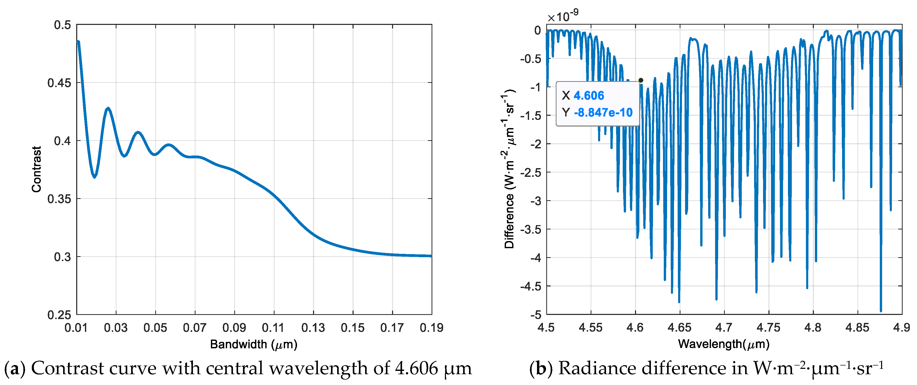
5.1.1. Carbon Monoxide (CO)

The CO density measured as the average per one hour is set as 5 mg∙m⁻³, which is the boundary between excellent and good in the AQI of mainland China. In contrast, the CO density is about 0.17–0.2 mg∙m⁻³ in the reference atmospheric models [65]. With the spectral reflectivity and emissivity of the land cover named urban and built-up [72], the spectral radiance curves of the unpolluted and the polluted atmosphere are calculated at 1 nm resolution in a spectrum spanning from 0.4 to 14 μm, as shown in Figure 2.

As it can be seen in Figure 2, molecular absorption occurs at a few specific bands, leading to the lower transmittance and the less intense total radiance, which can be used to identify the molecular species and retrieve density. Since these spectral characteristics distribute in a relatively narrow spectral range, the contrast can be analyzed in a narrower spectrum for efficiency.

With the assumption that the pollution covers an entire IFOV, the contrast and the SNR matrices are calculated for various bands in spectrum from 2.0 to 5.0 μm, as shown in Figure 3.

As it has been discussed in Section 4.2, the SNRs in Figure 3b are calculated using the unpolluted atmospheric condition. The bands whose corresponding SNRs are lower than the threshold are excluded directly in the optimal band selection. Besides, Figure 3 shows that the bands with higher contrasts may not obtain higher SNR.

The maximal contrast in Figure 3a is about 0.486, which is calculated at the central wavelength of 4.606 μm and the bandwidth of 0.01 μm. To figure out the effect of bandwidth on detection performance, the contrast curve calculated with the central wavelength of 4.606 μm and different bandwidths is given in Figure 4a, while Figure 4b is the spectral radiance around a wavelength of 4.606 μm.

Molecular absorption and emission occur at specific wavelength point characterized as spectral lines with extreme narrow width. However, due to molecular vibration and thermodynamic collision, the width of the spectral lines is broadened, resulting in a structure of the vibrational band of CO in the spectral radiance curves, as shown in Figure 2. When the central wavelength and the shape of the spectral filter are specified, the function of the spectral filter can be approximated as calculating the average difference in the specified band. As the widths of the spectral lines are generally much narrower than the bandwidth, a number of peaks and valleys are included in the calculation, leading to the fluctuation in Figure 4a.

In addition, because of the vibration phenomenon in Figure 4b, a narrower band is expected to achieve higher contrast, while the central wavelength of the optimal band is related to the available minimal bandwidth set in Table 2. For example, regarding the spectral radiance curves in Figure 2, when the minimal bandwidth is set as 0, 0.02, and 0.10 μm, the optimal bands are, respectively, 4.601–4.611 μm, 4.600–4.620 μm, and 4.545–4.645 μm. The corresponding contrasts are 0.486, 0.445, and 0.3749. The results are consistent with the band adopted in [38], where the band for CO detection is centered at 4.60 μm with about 0.12 μm bandwidth (4.545–4.665 μm).

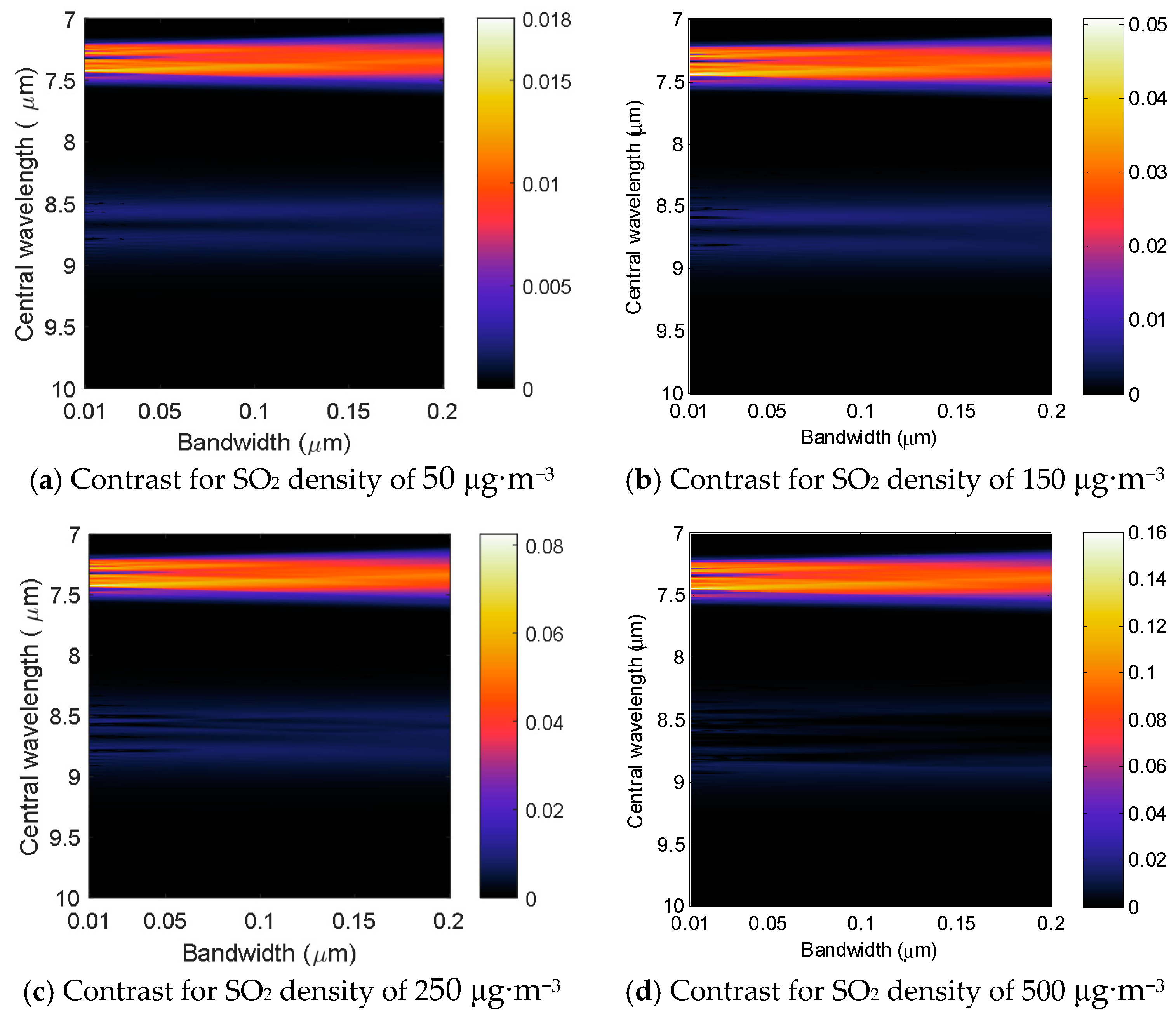
5.1.2. Sulfur Dioxide (SO₂)

Similar to the discussion about the optimal band for CO detection, the SO₂ boundary density between excellent and good in the AQI of mainland China is selected as an example, which is 150 μg∙m⁻³ measured as average per one hour. In contrast, the performance of the bands in Table 2 is also analyzed for the SO₂ density of 50 μg∙m⁻³ (excellent), 250 μg∙m⁻³ (good) and 500 μg∙m⁻³ (lightly polluted) to illustrate the effects of pollutant density. The results are shown in Figure 5, where the contrast is assigned as zero when the SNR of the corresponding band is lower than the threshold.

As another type of gaseous pollutant, the procedure of optimal band analysis for SO₂ is almost the same with CO. Figure 5 shows that the central wavelength of the optimal band locates at 7.2–7.5 μm. When the available minimal bandwidth is set as 0.01 μm, the optimal bands are the same for the two given densities, which locates at the central wavelength of 7.436 μm with the bandwidth of 0.011 μm. Although the exact same optimal band for different densities can be coincident, it indicates that the contrasts in different bands are close to each other in a small range of central wavelengths and bandwidths. For instance, in Figure 5b, the contrast in the bands 7.431–7.441 μm and 7.431–7.442 μm are, respectively, 0.0505 and 0.0508, which have negligible difference for detection. In comparison, a wider band was used to detect SO₂ plume from Mt. Etna volcano in [36], where the band was located at 1285–1345 cm⁻¹ (around 7.435–7.782 μm).

Note that detection of SO₂ is more challenging than CO since the contrasts in Figure 6 is much lower than Figure 5, while the proposed procedure can potentially be used for regions with relatively low concentrations of pollutants (the corresponding AQI in Figure 5a is lower than 20).

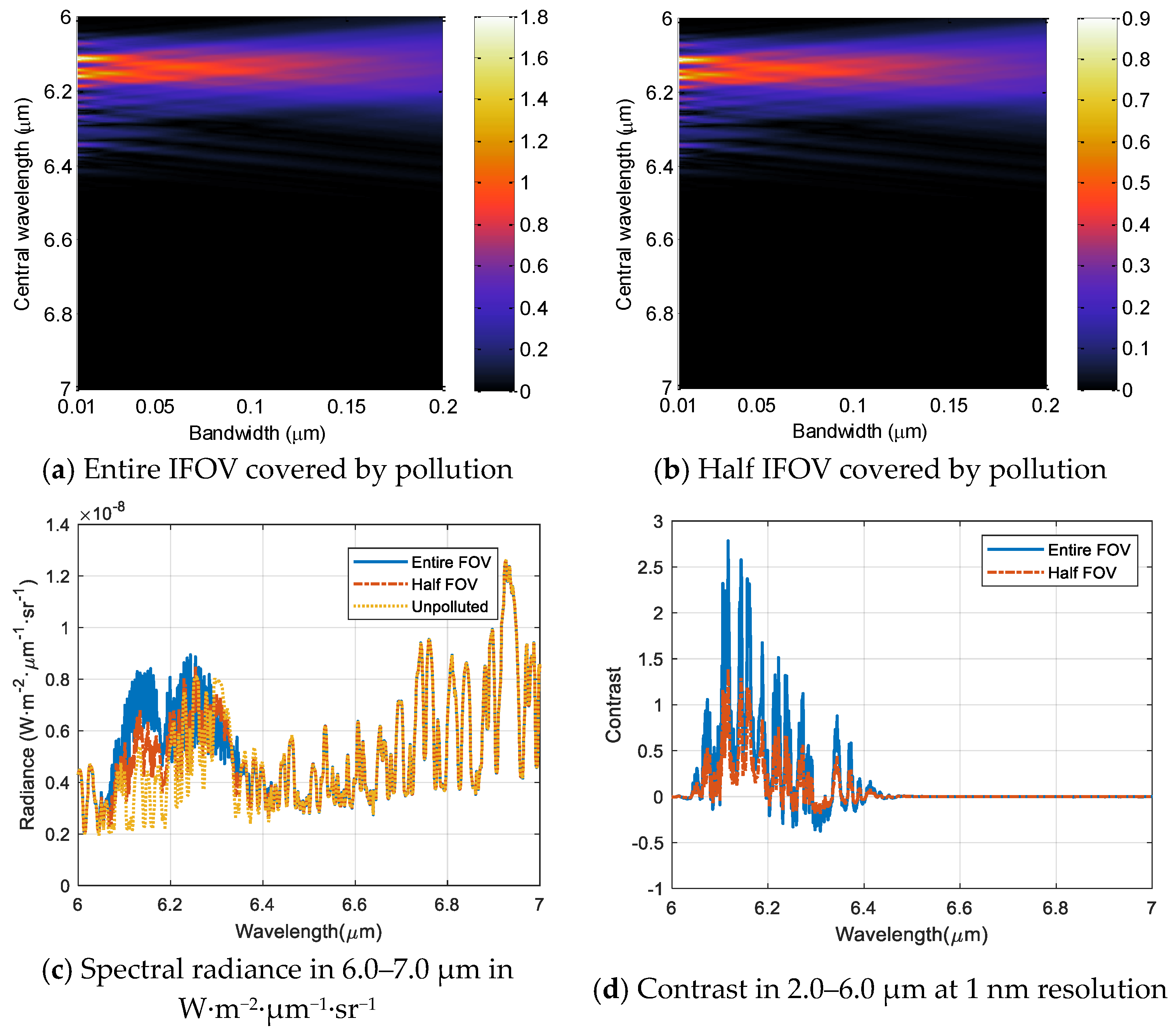
5.1.3. Nitrogen Dioxide (NO₂)

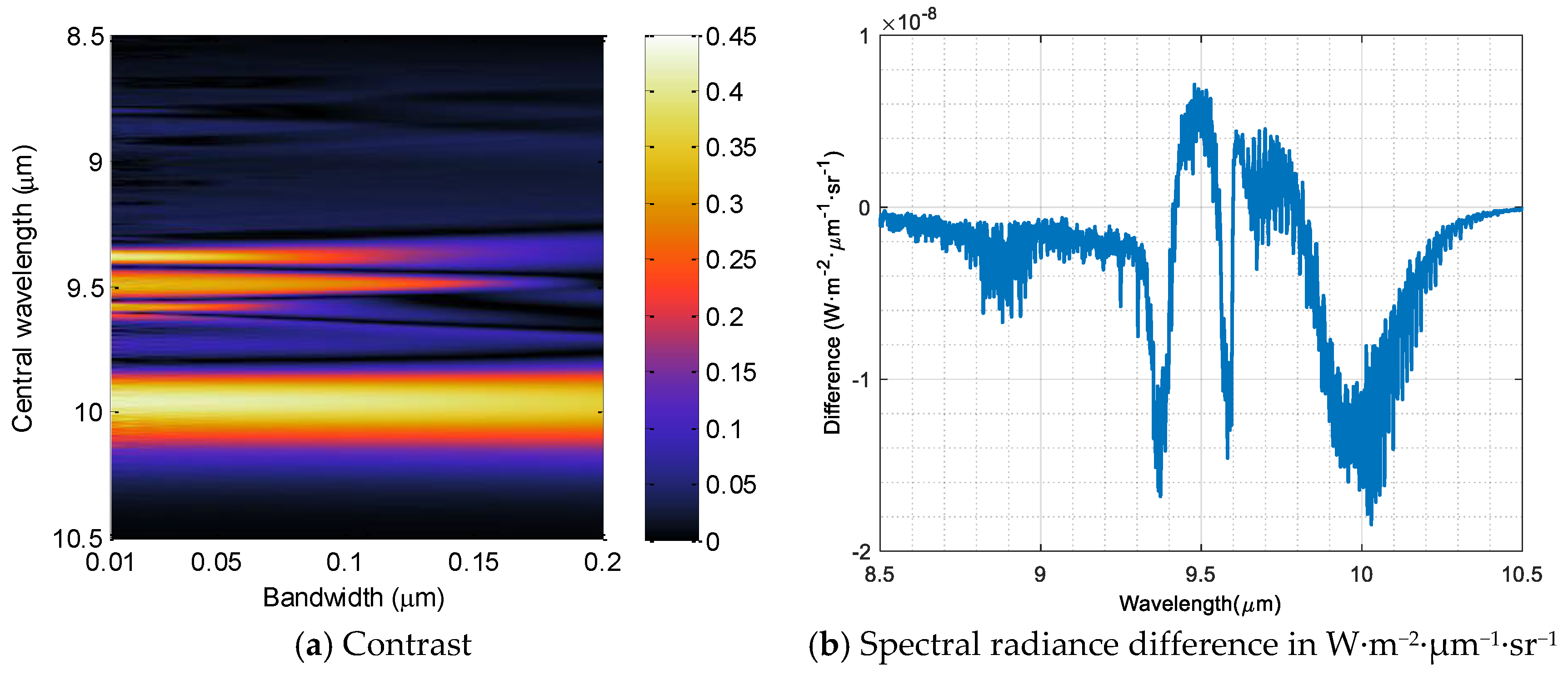
The density boundary of excellent and good AQI for NO₂ is 100 μg∙m⁻³ measured as average per one hour, in contrast with 0.04–0.05 μg∙m⁻³ in the reference atmospheric models. The contrast matrices of different pollution areas are calculated and given in Figure 6.

As can be seen in Equation (19) (similar to the Equation (13) in [56]), the contrast depends on two ratios, i.e., the ratio of solid angles and the ratio of radiances. The solid angle ΔΩ_t is related to the pollution area, whereas the spectral radiances E_g, E_p and E′_p indicate radiation flux in unit area at specific wavelength (in unit of W∙m⁻²∙μm⁻¹). Consequently, the pollution area has noticeable impacts on the contrast value, whereas it has no effect on the optimal center wavelength or bandwidth. As can be seen in Figure 6, the patterns of Figure 6a,b show no obvious difference. Although it is easy to identify different spectral radiance curves in Figure 6c, the contrast for pollution covering entire FOV is twice of the contrast for pollution covering half FOV.

Regarding the specified conditions, the optimal band for NO₂ detection locates at the wavelength of 6.112 μm with the bandwidth of 0.013 μm. The result is similar to the band for NO₂ measurement in [70], which centered at 1632.1 cm⁻¹ with 1 cm⁻¹ bandwidth (6.125–6.129 μm).

The relationship between the available minimal bandwidth and the selected optimal band has been discussed thoroughly in Section 5.1.1 and Section 5.1.2.

5.1.4. Ozone (O₃)

The vertical density distribution of O₃ is different than the three above-mentioned gaseous pollutants. As can be seen in Figure 7, the maximum of O₃ density in each reference atmospheric model appears around the height of 20 km, whereas the density of CO decreases with height [65].

The O₃ density is set as 160 μg∙m⁻³ at the ground, in contrast with a maximal density of 50–60 μg∙m⁻³ in the six types of reference models. The performance of various bands for O₃ detection is given in Figure 8, where Figure 8a is the contrast matrix while Figure 8b is the spectral radiance difference between the polluted and unpolluted atmospheric conditions.

As can be seen Figure 8b, the spectral radiance difference between the O₃ contaminated atmosphere and the unpolluted atmosphere can be either positive or negative in the given spectrum. This phenomenon is related to many influencing factors, including ozone concentration, ground emissivity and temperature, and temperature gradients between the stratospheric ozone layer and tropopause. When the ozone concentration increases, the atmospheric radiance becomes more intense while the ground radiance is weaker. As the total spectral radiance varies nonlinearly with the ozone concentration, both positive and negative values can be seen in the difference.

As the spectral filtering actually calculates the average difference in the specific bands, the optimal band can be selected via accumulating either positive or negative values of the radiance difference. Regarding the specified conditions, the optimal band for O₃ detection locates at the wavelength of 9.967 μm with the bandwidth of 0.010 μm. The optimal band is still related to the available minimal bandwidth. When the available minimal bandwidth is set as 1.084 μm, the optimal band is 9.289–10.369 μm with a maximal contrast of 0.1205. A similar spectral band was used in [71], where the spectral range for retrieval ozone concentration is 970 cm⁻¹ through 1084 cm⁻¹ (around 9.225–10.309 μm with contrast about 0.1169).

According to the results and discussions in Section 5.1, gaseous pollutants can be detected using the bands affected by molecular absorption phenomenon, where variance of total radiance at sensor aperture is identified for pollutant detection. Although the optimal band of each gaseous pollutant is related to available minimal band and pollutant density, the bands at the nearby central wavelength with similar bandwidth can achieve equivalent detection performance, since the contrast difference is negligible. Besides, detection performance can probably be improved using a narrower bandwidth.

It should be noted that the SNR threshold is set to exclude low SNR bands before the implementation of optimal band selection. This step ensures that the selected bands can measure data in unpolluted regions. The impacts of SNR will be discussed in more detail in the following section.

5.2. Aerosol Particles

The aerosol density is generally measured using bands without absorption effect, such as 0.55 and 0.6 μm. However, it is difficult to identify the type of aerosol for pollutant detection. With the assumption that the aerosol density can be retrieved by means of visibility estimation, the possibility of aerosol type identification is discussed in this section.

The spectral radiance of rural aerosol with 12 km visibility is calculated in comparison with the spectral radiance of urban aerosol with the same visibility and ground cover. Since aerosol scattering phenomenon is noticeable in visible and short-wave infrared, the spectral radiance curves from 0.4 to 2.5 μm with the ground cover of urban and built-up [72] are calculated and plotted in Figure 9.

As can be seen in Figure 9, the total radiance through urban aerosol is weaker than rural aerosol in most bands, since the ground reflection is more intense than atmospheric scattering contribution to the radiance in this spectral range, where the impact of illuminating geometry on the total radiance is noticeable.

With the assumption that the aerosol pollutant covers an entire IFOV, the contrast and the SNR matrices are calculated for various bands in spectrum from 0.5 to 2.0 μm, as shown in Figure 10.

As can be seen in Figure 10a, the bands located around 1.4 and 1.8 μm seem to achieve better performance. However, either the spectral radiance in Figure 9a or the radiance difference in Figure 9b is extremely low in these spectral regions. The major reason for this difference is the lack of spectral contrast between surface and aerosol in urban areas for these bands. In this situation, the SNR of these bands should be considered to distinguish available detection bands, as shown in Figure 10b.

For reliable discrimination, the SNR threshold is set as 30 for optimal band selection while another set of geometry parameters are selected, i.e., solar zenith angle (RZA) of 50°, viewing zenith angle (VZA) of 30°, and relative azimuth angle (RAA) of 120°. The analyzing results are given in Figure 11.

The patterns of the two figures show similar characteristics in Figure 11. As has been discussed in Section 5.1, the optimal band is selected via maximizing the difference of the total radiance through urban aerosol to the total radiance through rural aerosol. For Figure 11a,b, the optimal bands are, respectively, 0.773–0.783 μm and 0.772–0.782 μm in comparison to 0.743–0.753 μm band used in the MODIS for retrieving aerosol properties. It still should be noticed that the nearby bands have similar performance for distinguishing aerosol types.

The discussion in this section demonstrates the importance of considering SNR in optimal band selection. As shown in Figure 11, some spectral bands can achieve high contrasts with extremely low SNRs, implying that the bands can measure nothing but noise in unpolluted regions. Consequently, the proposed procedure can potentially be applied to select remote sensing bands in regions with relatively low pollutant concentrations.

6. Conclusions

We propose a band selection procedure of space-based infrared sensors for urban air pollutant detection, which is based on contrast and SNR analyses. The fundamental model of atmospheric radiative transfer calculation is reviewed to clarify the theoretical relevance between the total radiance at the aperture of the space-based infrared sensor and the pollutant density. Instead of selecting bands for retrieving the atmospheric radiance from the total radiance, the contrast of the polluted area to the unpolluted area is calculated in various bands to characterize the sensitivity of the bands to the variance of the pollutant density. Then, with the consideration of the SNR threshold, the band achieving the maximal contrast is selected as the optimum.

To demonstrate the usefulness of the proposed procedure, the optimal bands are analyzed respectively for detecting four types of gaseous pollutants and discriminating aerosol particle pollution in the AQI estimation. As can be seen in the results, for gaseous pollutants including CO, SO₂, NO₂, and O₃, the radiance variance can be observed in a relatively narrow spectral range, in which a narrower band tends to achieve better performance. Due to the fact that the peaks and valleys in total radiance curves are caused by molecular vibration and collision, the optimal band is actually related to different factors including available minimal bandwidth, ground cover characteristics, and pollutant density. However, the bands located near the central wavelength of the optimum with a slight different bandwidth can achieve similar performance for pollutant detection. As a reference, with the limit of 0.01 μm available minimal bandwidth, the optimal bands for CO, SO₂, NO₂, and O₃ are around 4.601–4.611 μm, 7.431–7.442 μm, 6.106–6.119 μm, and 9.962–9.972 μm, respectively.

Besides, the possible band for discriminating different types of aerosol is analyzed under the same visibility with the consideration of impacts of geometry difference. The impacts of available minimal bandwidth and ground cover characteristics are similar to those in gaseous pollutant detection, whereas for some bands achieving higher contrasts, the corresponding SNRs are too low for reliable detection. With a specified SNR threshold, the optimal band is analyzed for distinguishing the urban aerosol from the rural aerosol, which is around 0.773–0.783 μm.

The physics-based analysis procedure can be used in space-based infrared sensor design, especially for acquiring available data in regions with relatively low pollutant concentrations. The procedure can also be used to retrieve pollutant concentrations in future studies.

References

1. Pope, C.A.; Burnett, R.T.; Thun, M.J.; Calle, E.E.; Krewski, D.; Ito, K.; Thurston, G.D. Lung Cancer, Cardiopulmonary Mortality, and Long-term Exposure to Fine Particulate Air Pollution. J. Am. Med. Assoc. 2002, 287, 1132–1141. [Google Scholar] [CrossRef] [PubMed] [Green Version]
2. Krewski, D.; Burnett, R.; Goldberg, M.; Hoover, B.K.; Siemiatycki, J.; Jerrett, M.; Abrahamowicz, M.; White, W. Overview of the Reanalysis of the Harvard Six Cities Study and American Cancer Society of Particulate Air Pollution and Mortality. J. Toxicol. Environ. Health Part A 2003, 66, 1507–1551. [Google Scholar] [CrossRef]
3. Martin, R.V. Satellite Remote Sensing of Surface Air Quality. Atmos. Environ. 2008, 42, 7823–7843. [Google Scholar] [CrossRef]
4. Gu, K.; Qiao, J.; Lin, W. Recurrent Air Quality Predictor Based on Meteorology- and Pollution-Related Factors. IEEE Trans. Ind. Informat. 2018, 14, 3946–3955. [Google Scholar] [CrossRef]
5. Jain, R.K.; Moura, M.F.J.; Kontokosta, C.E. Big Data + Big Cities: Graph Signals of Urban Air Pollution. IEEE Signal Process. Mag. 2014, 130, 130–136. [Google Scholar] [CrossRef]
6. Shaban, K.B.; Kadri, A.; Rezk, E. Urban Air Pollution Monitoring System with Forecasting Models. IEEE Sens. J. 2016, 16, 2598–2606. [Google Scholar] [CrossRef]
7. Kaufman, Y.J.; Tanre, D.; Boucher, O. A Satellite View of Aerosols in the Climate System. Nature 2002, 419, 215–223. [Google Scholar] [CrossRef]
8. Wang, J.; Christopher, S.A. Intercomparison between Satellite-derived Aerosol Optical Thickness and PM2.5 Mass: Implications for Air Quality Studies. Geophys. Res. Lett. 2003, 30. [Google Scholar] [CrossRef]
9. Donkelaar, A.V.; Martin, R.V.; Park, R.J. Estimating Ground-level PM2.5 Using Aerosol Optical Deth Determined from Satellite Remote Sensing. J. Geophys. Res. 2006, 111. [Google Scholar] [CrossRef]
10. Remer, L.A.; Kleidman, R.G.; Levy, R.C.; Kaufman, Y.J.; Tanre, D.; Mattoo, S.; Martins, J.V.; Ichoku, C.; Koren, I.; Yu, H.; et al. Global Aerosol Climatology from the MODIS Satellite Sensors. J. Geophys. Res. 2008, 113. [Google Scholar] [CrossRef]
11. Hoff, R.M.; Christopher, S.A. Remote Sensing of Particulate Pollution from Space: Have We Reached the Promised Land? J. Air Waste Manag. Assoc. 2009, 59, 645–675. [Google Scholar] [CrossRef] [PubMed]
12. Streets, G.D.; Canty, T.; Carmichael, G.R.; Foy, B.D.; Dickerson, R.R.; Duncan, B.N.; Edwards, D.P.; Haynes, J.A.; Henze, D.K.; Houyoux, M. Emission Estimation from Satellite Retrievals: A Review of Current Capability. Atmos. Environ. 2013, 77, 1011–1042. [Google Scholar] [CrossRef]
13. Abad, G.G.; Souri, A.H.; Bak, J.; Chance, K.; Flynn, L.E.; Krotkov, N.A.; Lamsal, L.; Li, C.; Liu, X.; Miller, C.C. Five Decades Observing Earth’s Atmospheric Trace Gases Using Ultraviolet and Visible Backscatter Solar Radiation from Space. J. Quant. Spectrosc. Radiat. Transf. 2019. [Google Scholar] [CrossRef]
14. Krueger, A.J. Sighting of El Chichon Sulfur Dioxide Clouds with the Nimbus 7 Total Ozone Mapping Spectrometer. Science 1983, 220, 1377–1379. [Google Scholar] [CrossRef] [PubMed]
15. Burrows, J.P.; Weber, M.; Buchwitz, M.; Rozanov, V.; Ladstatter-Werbenmayer, A.; Richter, A.; Debeek, R.; Hoogen, R.; Bramstedt, K.; Eichmann, K.; et al. The Global Ozone Monitoring Experiment (GOME): Mission Concept and First Scientific Results. J. Atmos. Sci. 1999, 56, 151–175. [Google Scholar] [CrossRef]
16. Bovensmann, H.; Burrows, J.P.; Buchwitz, M.; Frerick, J.; Noel, S.; Rozanov, V.V.; Chance, K.V.; Goede, A.O.H. SCIAMACHY: Mission Objectives and Measurement Modes. J. Atmos. Sci. 1999, 56, 127–150. [Google Scholar] [CrossRef] [Green Version]
17. Buchwitz, M.; Burrows, J.P. Retrieval of CH4, CO, and CO2 Total Column Amounts rom SCIAMACHY Near-infrared Nadir Spectra: Retrieval Algorithm and First Results. Proc. SPIE 2003, 5235, 375–388. [Google Scholar]
18. Ahmad, S.P.; Levelt, P.F.; Bhartia, P.K.; Hilsenrath, E.; Leppelmeier, G.W.; Johnson, J.E. Atmospheric Products from the Ozone Monitoring Instrument (OMI). Proc. SPIE 2003, 5151, 619–630. [Google Scholar]
19. Veefkind, J.P.; De Haan, J.F.; Brinksma, E.J.; Kroon, M.; Levelt, P.F. Total Ozone from the Ozone Monitoring Instrument (OMI) Using the DOAS Technique. IEEE Trans. Geosci. Remote Sens. 2006, 44, 1239–1244. [Google Scholar] [CrossRef]
20. Chance, K.; Liu, X.; Suleiman, M.; Flittner, D.E.; Al-Saddi, J.; Janz, S.J. Tropospheric Emissions: Monitoring of Pollution (TEMPO). Proc. SPIE 2013, 8866, 88660D. [Google Scholar]
21. Zoogman, P.; Liu, X.; Suleiman, R.M.; Pennington, W.F.; Flittner, D.E.; Al-Saadi, J.A.; Hilton, B.B.; Nicks, D.K.; Newchurch, M.J.; Carr, J.L. Tropospheric Emissions: Monitoring of Pollution (TEMPO). J. Quant. Spectrosc. Radiat. Transf. 2017, 186, 17–39. [Google Scholar] [CrossRef]
22. Ingmann, P.; Veihelmann, B.; Langen, J.; Lamarre, D.; Stark, H.; Courreges-Lacoste, G.B. Requirements for the GMES Atmosphere Service and ESA’s Implementation Concept: Sentinels-4/-5 and -5p. Remote Sens. Environ. 2012, 120, 58–69. [Google Scholar] [CrossRef]
23. Choi, W.J.; Moon, K.; Yoon, J.; Cho, A.; Kim, S.; Lee, S.; Ko, D.H.; Kim, J.; Ahn, M.H.; Kim, D. Introducing the geostationary environment monitoring spectrometer. J. Appl. Remote Sens. 2018, 12, 044005. [Google Scholar] [CrossRef]
24. Dobber, M.; Kleipool, Q.; Veefkind, P.; Levelt, P.; Rozemeijer, N.; Hoogeveen, R.; Aben, I.; de Vries, J.; Otter, G. From Ozone Monitoring Instrument (OMI) to Tropospheric Monitoring Instrument (TROPOMI). Proc. SPIE 2008, 10566, 105661Z. [Google Scholar]
25. Hebestreit, K.; Stutz, J.; Rosen, D.; Matveiv, V.; Peleg, M.; Luria, M.; Platt, U. DOAS Measurements of Tropospheric Bromine Oxide in Mid-Latitudes. Science 1999, 283, 55–57. [Google Scholar] [CrossRef] [PubMed]
26. Wagner, T.; Dix, B.; Friedeburg, C.V.; Frieβ, U.; Sanghavi, S.; Sinreich, R.; Platt, U. MAX-DOAS O4 Measurements: A New Technique to Derive Information on Atmospheric Aerosols—Principles and Information Content. J. Geophys. Res. 2004, 109. [Google Scholar] [CrossRef]
27. Bhartia, P.K. OMI Algorithm Theoretical Basis Document: Ume II OMI Ozone Products; ATBD-OMI-02, version 2.0; NASA Goddard Space Flight Center: Greenbelt, MD, USA, 2002. Available online: https://eospso.gsfc.nasa.gov/sites/default/files/atbd/ATBD-OMI-02.pdf (accessed on 4 July 2019).
28. Krotokov, N.A.; Carn, S.A.; Krueger, A.J.; Bhartia, P.K.; Yang, K. Band Residual Difference Algorithm for Retrieval of SO2 from the Aura Ozone Monitoring Instrument (OMI). IEEE Trans. Geosci. Remote Sens. 2006, 44, 1259–1266. [Google Scholar] [CrossRef]
29. Krotkov, N.A.; McClure, B.; Dickerson, R.R.; Cam, S.A.; Li, C.; Bhartia, P.K.; Yang, K.; Krueger, A.J.; Li, Z.; Levelt, P.F. Validation of SO2 Retrievals from the Ozone Monitoring Instrument Over NE China. J. Geophys. Res. 2008, 113. [Google Scholar] [CrossRef]
30. Remer, L.A.; Kaufman, Y.J.; Tanre, D.; Mattoo, S.; Chu, D.A.; Martins, J.V.; Li, R.R.; Ichoku, C.; Levy, R.C.; Kleidman, R.G. The MODIS Aerosol Algorithm, Products, and Validation. J. Atmos. Sci. 2005, 62, 947–973. [Google Scholar] [CrossRef] [Green Version]
31. Justice, C.O.; Vermote, E.; Townshend, J.R.G.; Defries, R.; Roy, D.P.; Hall, D.K.; Salomonson, V.V.; Privette, J.L.; Riggs, G.; Strahler, A. The Moderate Resolution Imaging Spectroradiometer (MODIS): Land Remote Sensing for Global Chance Research. IEEE Trans. Geosci. Remote Sens. 1998, 36, 1228–1249. [Google Scholar] [CrossRef]
32. Pagano, T.S.; Durham, R.M. Moderate Resolution Imaging Spectroradiometer (MODIS). Proc. SPIE 1993, 1939, 2–17. [Google Scholar]
33. Liu, Z.; Hunt, W.H.; Young, S.A. Overview of the CALIPSO Mission and CALIOP Data Processing Algorithms. J. Atmos. Ocean. Tech. 2009, 36, 2310–2323. [Google Scholar]
34. Jethva, H.; Torres, O.; Remer, L.A.; Bhartia, P.K. A Color Ratio Method for Simultaneous Retrieval of Aerosol and Cloud Optical Thickness of Above-Cloud Absorbing Aerosols from Passive Sensors: Application to MODIS Measurements. IEEE Trans. Geosci. Remote Sens. 2013, 51, 3862–3870. [Google Scholar] [CrossRef]
35. Liu, Y.; Park, R.J.; Jacob, D.J.; Li, Q.; Kilaru, V.; Sarnat, J.A. Mapping Annual Mean Ground-level PM2.5 Concentrations Using Multiangle Imaging Spectroradiometer Aerosol Optical Thickness over the Contiguous United States. J. Geophys. Res. 2004, 109, D22206. [Google Scholar]
36. Strow, L.L.; De Souza-Machado, S.; Edomonds, Y.; Hannon, S. Quantifying Tropospheric canic Emissions with AIRS: The 2002 Eruption of Mt. Etna (Italy). Geophys. Res. Lett. 2005, 32. [Google Scholar] [CrossRef]
37. Teggi, S.; Bogliolo, M.P.; Buongiorno, M.F.; Pugnaghi, S.; Sterni, A. Evaluation of SO2 Emission from Mount Etna Using Diurnal and Nocturnal Multispectral IR and Visible Imaging Spectrometer Thermal IR Remote Sensing Images and Radiative Transfer Models. J. Geophys. Res. 1999, 104, 20069–20079. [Google Scholar] [CrossRef]
38. Smith, M.W.; Shertz, S.R.; Delen, N. Remote Sensing of Atmospheric Carbon Monoxide with the MOPITT Airborne Test Radiometer (MATR). Proc. SPIE 1999, 3756, 475–485. [Google Scholar]
39. Manolakis, D.; Truslow, E.; Pieper, M.; Cooley, T.; Brueggeman, M. Detection Algorithms in Hyperspectral Imaging Systems: An Overview of Practical Algorithms. IEEE Signal Process. Mag. 2014, 31, 24–33. [Google Scholar] [CrossRef]
40. Lopez, S.; Vladimirova, T.; Gonzalez, C.; Resano, J.; Mozos, D.; Plaza, A. The Promise of Reconfigurable Computing for Hyperspectral Imaging Onboard Systems: A Review and Trends. Proc. IEEE 2013, 191, 698–722. [Google Scholar] [CrossRef]
41. Bioucas-Dias, J.M.; Plaza, A.; Camps-Valls, G.; Scheunders, P.; Nasrabadi, N.M.; Chanussot, J. Hyperspectral Remote Sensing Data Analysis and Future Challenges. IEEE Geosci. Remote Sens. Mag. 2013, 1, 6–36. [Google Scholar] [CrossRef]
42. Lee, Z.; Carder, K.; Arnone, R.; He, M. Determination of Primary Spectral Bands for Remote Sensing of Aquatic Environments. Sensors 2007, 7, 3428–3441. [Google Scholar] [CrossRef] [PubMed] [Green Version]
43. Zhu, J.; Liu, W.; Liu, J.; Lu, Y.; Gao, M.; Xu, L.; Zhang, T.; Wei, X. FTIR Measurement and Analysis Based on the Selection of Optimized Spectral band. Spectrosc. Spectr. Anal. 2007, 27, 679–682. [Google Scholar]
44. Valor, E.; Caselles, V.; Coll, C.; Rubio, E.; Sospedra, F. NEDT Influence in Thermal Band Selection of Satellite-borne Instruments. Int. J. Remote Sens. 2002, 23, 3493–3504. [Google Scholar] [CrossRef]
45. Clodius, W.B.; Weber, P.G.; Borel, C.C.; Smith, B.W. Multi-spectral Band Selection for Satellite-based Systems. Proc. SPIE 1998, 3377, 11–21. [Google Scholar]
46. Price, J.C. Spectral Band Selection for Visible-Near Infrared Remote Sensing: Spectral-Spatial Resolution Tradeoffs. IEEE Trans. Geosci. Remote Sens. 1997, 35, 1277–1285. [Google Scholar] [CrossRef]
47. Stair, A.T., Jr. MSX Design Parameters Driven by Targets and Backgrounds. J. Hopkins APL Tech. Dig. 1996, 17, 11–18. [Google Scholar]
48. Price, J.C. Band Selection Procedure for Multispectral Scanners. Appl. Opt. 1994, 33, 3281–3288. [Google Scholar] [CrossRef]
49. Berk, A.; Conforti, P.; Kennett, R.; Perkins, T.; Hawes, F.; van den Bosch, J. MODTRAN 6: A Major Upgrade of the MODTRAN Radiative Transfer Code. Proc. SPIE 1998, 90880H. [Google Scholar] [CrossRef]
50. Guanter, L.; Richter, R.; Kaufmann, H. On the Application of the MODTRAN4 Atmospheric Radiative Transfer Code to Optical Remote Sensing. Int. J. Remote Sens. 2009, 30, 1407–1424. [Google Scholar] [CrossRef]
51. Clough, S.A.; Shephard, M.W.; Mlawer, E.J.; Delamere, J.S.; Iacono, M.J.; Cady-Pereira, K.; Boukabara, S.; Brown, P.D. Atmospheric Radiative Transfer Modeling: A Summary of the AER Codes. J. Quant. Spectrosc. Radiat. Transf. 2005, 91, 233–244. [Google Scholar] [CrossRef]
52. Chen, W.; Xu, X. Spectral Resolution Enhancement for SBDART. IEEE Congr. Image Signal Process. 2008, 5, 523–527. [Google Scholar]
53. He, X.; Xu, X. Contrast Analysis of Space-based of Earth Observational Infrared System. Proc. SPIE 2014, 9249, 92490F. [Google Scholar]
54. Shi, X.; Xu, X. Impact of Background Radiation on the Detection Performance of Interceptor Seekers. J. Syst. Eng. Electron. 2010, 32, 2053–2056. [Google Scholar]
55. He, X.; Xu, X. Physically Based Model for Multispectral Image Simulation of Earth Observation Sensors. IEEE J. Sel. Top. Appl. Earth Obs. Remote Sens. 2017, 10, 1897–1908. [Google Scholar] [CrossRef]
56. He, X.; Xu, X. Optimal Band Analysis for Dim Target Detection in Space-variant Sky Background. Proc. SPIE 2018, 10795, 107950N. [Google Scholar]
57. Kesbava, N.; Mustard, J.F. Spectral Unmixing. IEEE Signal Process. Mag. 2002, 19, 44–57. [Google Scholar] [CrossRef]
58. Bioucas-Dias, J.M.; Plaze, A.; Dobigeon, N.; Parente, M.; Du, Q.; Garder, P.; Chanussot, J. Hyperspectral Unmixing Overview: Geometrical, Statistical, and Spares Regression-Based Approaches. IEEE J. Sel. Top. Appl. Earth Obs. Remote Sens. 2012, 50, 354–379. [Google Scholar] [CrossRef]
59. Cooke, B.J.; Lomheim, T.S.; Laubscher, B.E.; Rienstra, J.L.; Clodius, W.B.; Bender, S.C.; Weber, P.G.; Smith, B.W.; Vampola, J.L.; Claassen, P.J. Modeling the MTI Electro-Optic System Sensitivity and Resolution. IEEE Trans. Geosci. Remote Sens. 2005, 43, 1950–1962. [Google Scholar] [CrossRef]
60. Curtis, A.R. Discussion of a Statistical Model for Water Vapour Absorption. Q. J. R. Meteorol. Soc. 1952, 78, 638–640. [Google Scholar]
61. Godson, W.L. The Evaluation of Infrared-Radiative Fluxes due to Atmospheric Water Vapour. Q. J. R. Meteorol. Soc. 1953, 79, 367–379. [Google Scholar] [CrossRef]
62. Thalman, R.; Zarzana, K.; Tolbert, M.A.; Kamer, R. Rayleigh Scattering Cross-section Measurements of Nitrogen, Argon, Oxygen and Air. J. Quant. Spectrosc. Radiat. Transf. 2014, 147, 171–177. [Google Scholar] [CrossRef]
63. Gordon, I.E.; Rothman, L.S.; Hill, C.; Kochanov, R.V.; Tan, Y.; Bernath, P.F.; Birk, M.; Boudon, V.; Campargue, A.; Chance, K.V. The HITRAN2016 Molecular Spectroscopic Database. J. Quant. Spectrosc. Radiat. Transf. 2017, 203, 3–69. [Google Scholar] [CrossRef]
64. Rothman, L.S.; Pinsland, C.P.; Goldman, A.; Massie, S.T.; Edwards, D.P.; Flaud, J.M.; Perrin, A.; Camy-peyret, C.; Dana, V.; Mandin, J.Y. The HITRAN Molecular Spectroscopic Database and HAWKS (HITRAN Atmospheric Workstation): 1996 Edition. J. Quant. Spectrosc. Radiat. Transf. 1998, 60, 665–710. [Google Scholar] [CrossRef]
65. Anderson, G.P.; Chetwynd, J.H.; Clough, S.A.; Shettle, E.P.; Kneizys, F.X. AFGL Atmospheric Constituent Profiles (0–120 km); AFGL-TR-86-0110; Air Force Geophysics Laboratory: Hanscom AFB, MA, USA, 1986. [Google Scholar]
66. Wiscombe, W.J. Improved Mie Scattering Algorithms. Appl. Opt. 1980, 19, 1505–1509. [Google Scholar] [CrossRef] [PubMed]
67. Shettle, E.P.; Fenn, R.W. Models for the Aerosols of the Lower Atmosphere and the Effects of Humidity Variations on Their Optical Properties; AFGL-TR-79-0214; Air Force Geophysics Laboratory: Hanscom AFB, MA, USA, 1979. [Google Scholar]
68. Cao, J.; Wang, Q.; Chow, J.; Watson, J.G.; Tie, X.; Shen, Z.; Wang, P.; An, Z. Impacts of Aerosol Compositions on Visibility Impairment in Xi’an, China. Atmos. Environ. 2012, 59, 559–566. [Google Scholar] [CrossRef]
69. Koffi, B.; Schulz, M.; Breon, F.; Dentener, F.; Steensen, B.M.; Griesfeller, J.; Winker, D.; Balkanski, Y.; Bauer, S.E.; Bellouin, N. Evaluation of the Aerosol Vertical Distribution in Global Aerosol Models through Comparison against CALIOP Measurements: AeroCom Phase II Results. J. Geophys. Res. Atmos. 2015, 121, 7254–7283. [Google Scholar] [CrossRef]
70. Yamamoto, Y.; Sumizawa, H.; Yamada, H.; Tonokura, K. Real-time Measurement of Nitrogen Dioxide in Vehicle Exhaust Gas by Mid-Infrared Cavity Ring-down Spectroscopy. Appl. Phys. B 2011, 105, 923–931. [Google Scholar] [CrossRef]
71. Lightner, K.J.; McMillan, W.W.; McCann, K.J.; Hoff, R.M.; Newchurch, M.J.; Hinsta, E.J.; Barnet, C.D. Detection of a Tropospheric Ozone Anomaly Using a Newly Developed Ozone Retrieval Algorithm for an Up-looking Infrared Interferometer. J. Geophys. Res. 2009, 114, D06304. [Google Scholar] [CrossRef]
72. Loveland, T.R.; Reed, B.C.; Brown, J.F.; Ohlen, D.O.; Zhu, Z.; Yang, L.; Merchant, J.W. Development of a Global Land Cover Characteristics Database and IGBP DISCover from 1 km AVHRR Data. Int. J. Remote Sens. 2000, 21, 1303–1330. [Google Scholar] [CrossRef]
Figure 1. Flow chart for optimal band selection for urban pollutant detection.
Atmosphere 10 00631 g001
Figure 2. Spectral radiance at sensor aperture through unpolluted and CO contaminated atmospheres.
Atmosphere 10 00631 g002aAtmosphere 10 00631 g002b
Figure 3. Performance of various bands for CO detection (density of 5 mg∙m−3).
Atmosphere 10 00631 g003
Figure 4. Impacts of bandwidth on CO detection and explanation.
Atmosphere 10 00631 g004
Figure 5. Performance of various bands for SO2 detection in different densities.
Atmosphere 10 00631 g005
Figure 6. Performance of various bands for NO2 detection with different polluted areas (density of 100 μg∙m−3).
Atmosphere 10 00631 g006
Figure 7. Comparison of vertical density distribution of different gases [65].
Atmosphere 10 00631 g007
Figure 8. Performance of various bands for O3 detection.
Atmosphere 10 00631 g008
Figure 9. Spectral radiance at sensor aperture through different types of aerosol with same visibility.
Atmosphere 10 00631 g009
Figure 10. Performance of various bands for aerosol type discrimination (visibility of 12 km).
Atmosphere 10 00631 g010
Figure 11. Contrast matrices for aerosol type discrimination under different observation geometry.
Atmosphere 10 00631 g011