A Wind Tunnel Study on the Correlation between Urban Space Quantification and Pedestrian–Level Ventilation

Abstract

Correlation research on urban space and pedestrian–level wind (PLW) environments is helpful for improving the wind comfort in complex urban space. It could also be significant for building and urban design. Correlation research is usually carried out in a space with clear urban spatial characteristics, so it is necessary to define the space first. In this paper, a typical urban area in Nanjing, China, is selected as the research object, and a spatial partition method is used to divide the real complex urban space into subspaces. The urban spatial characteristics of such subspaces are quantified using three urban spatial indices: openness (O), area (A), and shape (S). By comparing the quantitative results, 24 (12 pairs) subspaces with prominent urban spatial indices are selected as the correlation research cases. The 24 subspaces also provide a reference for the layout of the measurement points in a wind tunnel experiment. This is a new arrangement for locating the measurement points of a wind tunnel for correlation research. In the experiment, 45 measurement points are located, and the mean wind velocity of four different wind directions at 45 measurement points is experimented. The results clearly show that, when the experimental conditions are the same, the changes of mean wind velocity ratio ($\overline{{\mathrm{U}}_{\mathrm{R}}}$) of 24 (12pairs) subspaces under the four experimental wind directions are close. The $\overline{{\mathrm{U}}_{\mathrm{R}}}$s of the subspaces are not significantly affected by the wind direction, which is affected more by the subspaces’ spatial characteristics. When making the correlation analysis between mean wind speed ratio and spatial characteristics’ indices, a direct numerical comparison was not able to find a correlation. By comparing the difference values of mean wind speed (△$\overline{{\mathrm{U}}_{\mathrm{R}}}$) and indices between each pair of subspaces, the correlation between $\overline{{\mathrm{U}}_{\mathrm{R}}}$ and openness of subspaces were found. Limited by spatial partition method, the correlation between $\overline{{\mathrm{U}}_{\mathrm{R}}}$ and the other indices was not obvious.

1. Introduction

The change of urban space and textures affects the microclimate [1,2]. With increasing urbanization, the ventilation problem caused by complex urban spaces is becoming more and more serious [3]. Research on the correlation between urban space and pedestrian level wind (PLW) can help prevent poor ventilation caused by complex urban spaces and improve the urban PLW environment [4]. Therefore, it is very important for designers to understand how urban spaces change the wind environment in the early stage of designing urban spaces [5,6]. This requires an intuitive method for studying the correlation between PLW environment and urban space. [7,8,9].

At present, the methods used to study wind environment mainly include field and wind tunnel experiments, as well as computational fluid dynamics (CFD) simulations. With the rapid development of computer technology, CFD has become a relatively convenient and effective technical means to study urban wind environment. However, the accuracy of CFD needs to be further verified [10,11,12]. Wind tunnel experiments are not only fundamental for studying wind environments, but also provide data to verify CFD simulations [11,13,14]. The wind environments around buildings and pedestrians constitute a significant concern, and the dependent wind tunnel experiments were not developed until 1965 [15]. PLW was proposed by Lawson in 1973, mainly to study the influence of pedestrian-height wind on people [16]. The wind tunnel experiment technologies, used to study the PLW environment, can be grouped into two categories: “point method” and “area method” [11,17].

In the wind tunnel experiment using “point method,” a suitable arrangement for the measurement points must be selected. The arrangement and number of measurement points, and the accuracy of measurement technologies need to be carefully considered, in order to avoid significant intrusive effects on the wind field [17]. There are four main arrangements of the wind tunnel measurement points. Some researchers have utilized “arrays” to predict the impact on a wind environment of proposed buildings in the surrounding areas [18,19] (Figure 1a). Some researchers have utilized “along streets” to study the distribution of wind in the height direction in the streets [20,21] (Figure 1b). Some researchers have utilized “around buildings” arrangements to study a wind environment around buildings [19,22,23] (Figure 1c). Some researchers have utilized “distributed” arrangements to perform the wind environment assessment for built-up areas [24,25] (Figure 1d). In the wind tunnel experiments, authors have used different arrangements of measurement points for different research objectives [18,19,20,21,22,23,24,25].

These four main arrangements of measurement points take into consideration some urban spatial characteristics (such as streets), but because their research purpose is not based on the characteristics of the urban space, the arrangements do not fully reflect the characteristics of the urban space. If the measurement points are laid out in accordance with the common modes, the number of measurement points will be excessive and interference between the experimental probes may occur. Errors in the determination of the urban spatial characteristics in the measurement point arrangements, will make it difficult to analyze the experiment results with respect to correlations. Beyond that, the wind tunnel experiment is affected by time, cost, and operability. It also has some other challenges, such as logistical support difficulties, data quality issues, and problems with spatial representativeness [26]. In the wind tunnel experiment of PLW, the spatial characteristics of several existing arrangements are less considered, which makes it difficult to analyze the experimental results based on the correlation. Therefore, for correlation research, it is necessary to locate measurement points from the perspective of urban spatial characteristics. Meanwhile, in the research on the correlation between urban spaces and wind environments, wind environment analysis is usually conducted in designated spaces [27,28,29]. When the research area is a large real urban area, with a complex and disordered space, it is necessary to ‘define’ the space first before conducting the correlation study.

Therefore, the present study uses the current knowledge of the urban space to divide the urban area into identified subspaces. Then the spatial characteristics of the subspaces can be determined, which are quantified by urban indices that are defined in Section 2.2. The quantification results not only provide a reference for the wind tunnel measurement points arrangement, but also provide a basis for correlation analysis. Based on this, the correlation between the spatial quantization results and the wind tunnel experiment results can be analyzed.

Section 2 provides a description of the wind tunnel experiment and the measurement point arrangement, based on correlation research. Section 3 provides the results and discussion. Section 4 draws the conclusions.

2. Methods

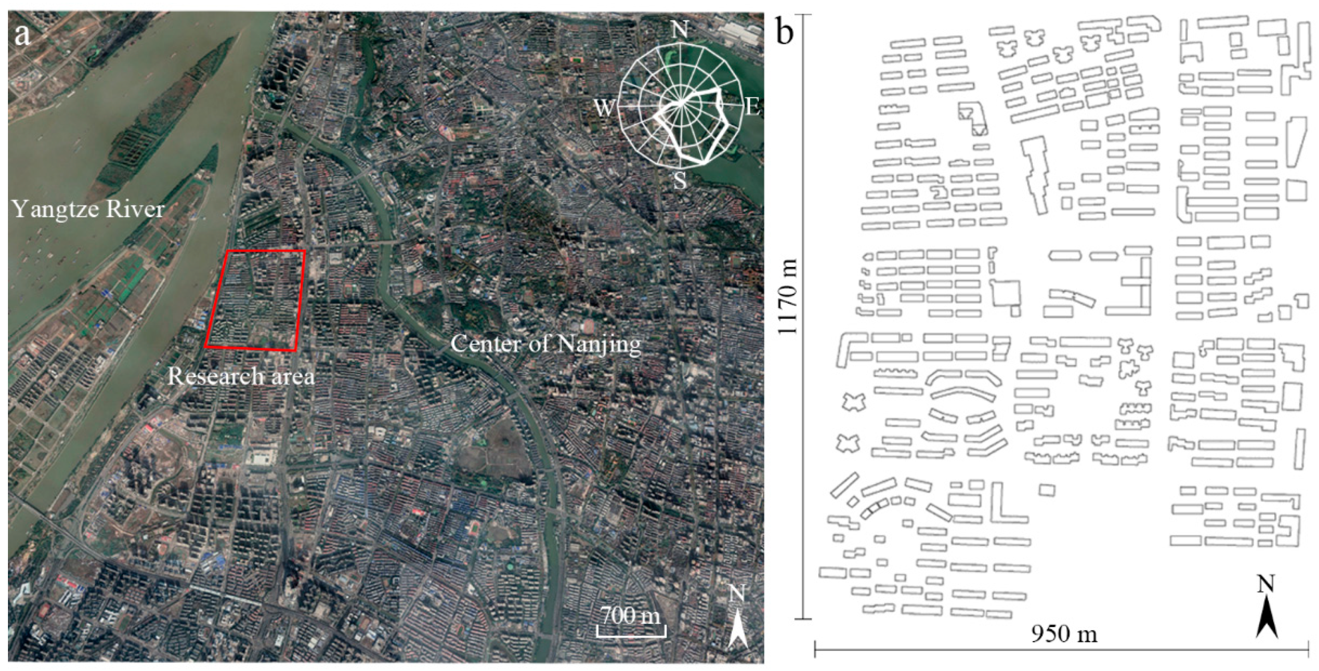
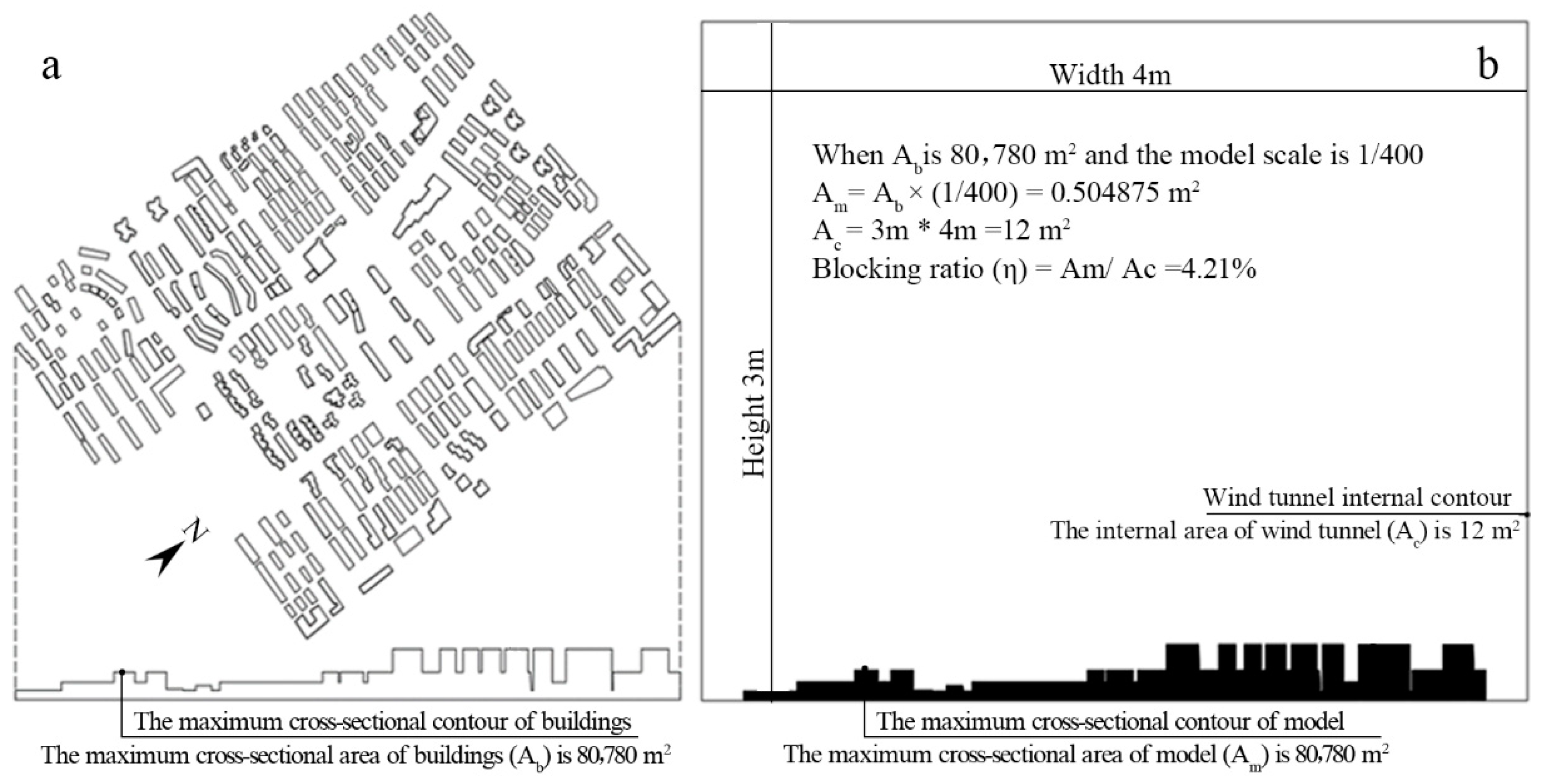
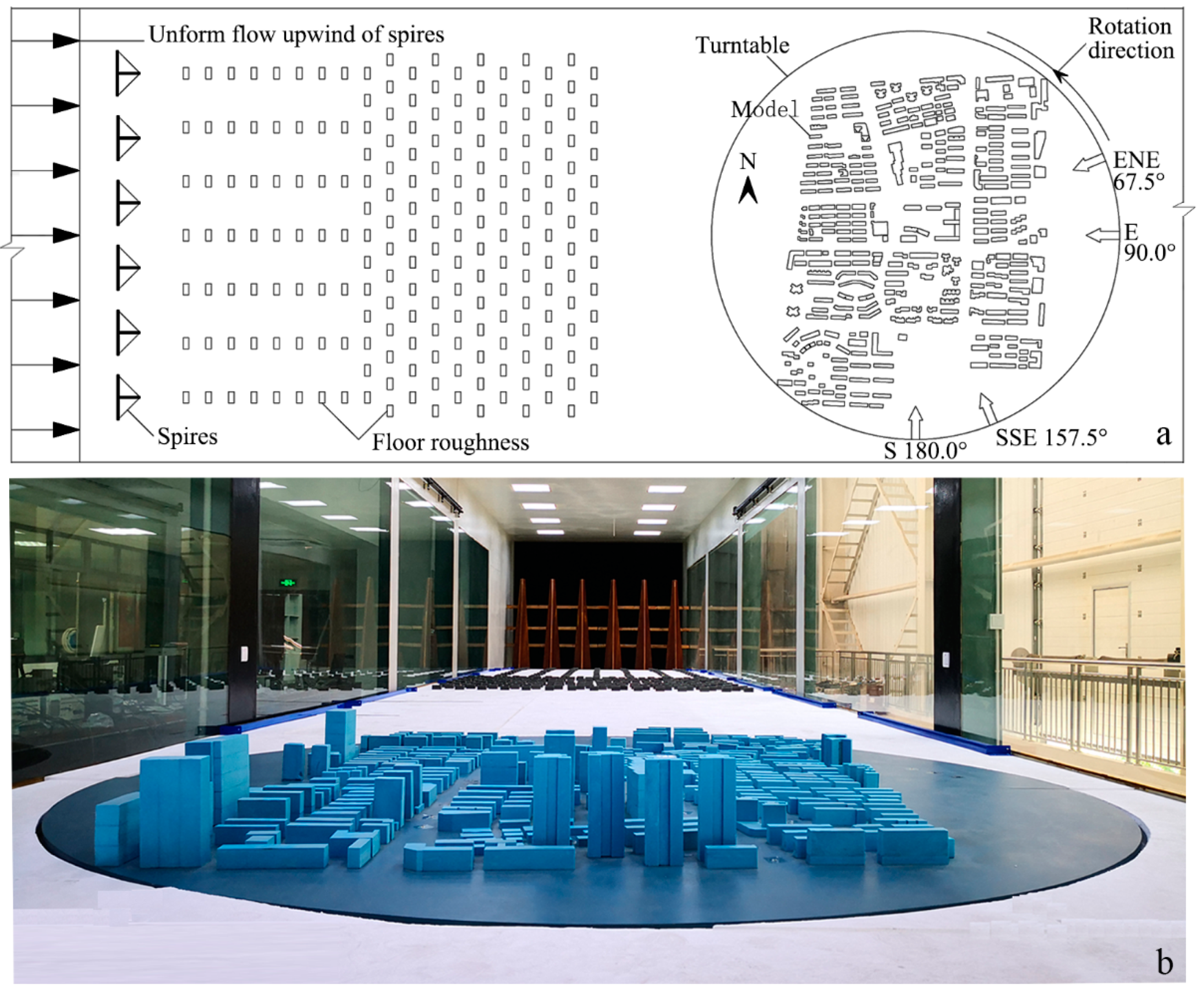
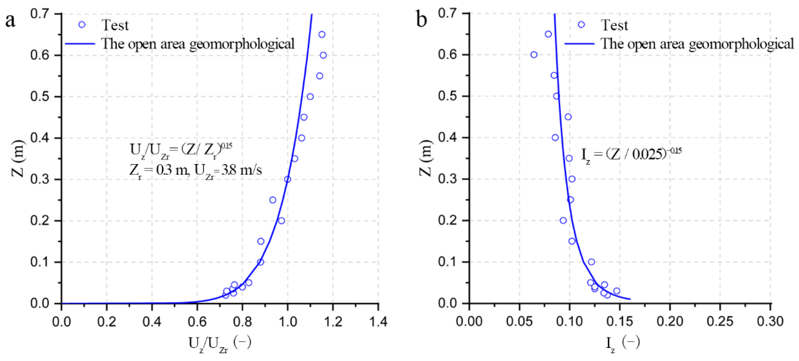
2.1. Description of the Research Area and the Wind Tunnel Experiment

In order to study the correlation between urban spatial characteristics and the PLW environment more accurately, the study area should not only contain various urban spaces with different spatial characteristics, but also be large enough for the analysis. [30,31]. Based on this, the research area is a typical urban area in Nanjing, which is a main city in an economically advanced area of China. The wind rise of Nanjing shown in Figure 2a, and the predominant wind direction in summer is SSE [32]. The west side of the research area contains the Yangtze River, and the east side is next to the center of Nanjing (Figure 2a). The east–west width is 950 m, and the north–south width is 1170 m. In such a large real urban area, the complexity and disorder of the space is obvious (Figure 2b).

The wind tunnel experiments were performed in a back-flow, atmospheric boundary-layer wind tunnel, which has the characteristics of a large experimental section size, excellent airflow performance, and can be operated in a closed-circuit back-flow mode or open-circuit direct-flow mode [33]. The experimental section size of the wind tunnel was 24 m × 4 m × 3 m (length × width × height). The diameter of the turntable was 3.6 m. The atmospheric boundary-layer simulation of the wind field adopted a system consisting of a three-dimensional moving coordinate frame and a hotline anemometer for the measurements. The hotline anemometer is calibrated beforehand. By measuring the distribution of the wind speed at different heights, the mean wind speed profile and turbulence intensity profile of the simulated flow field in the wind tunnel were obtained. The Irwin probe, one kind of “point method,” was used in the experiment; it has no directional sensitivity [34]. There is a quantitative relationship between the wind velocity at the steel needle of the probe tube and the pressure difference between the steel needle and the cavity. By measuring the pressure at the steel needle and the cavity, the wind velocity at the pedestrian height can be obtained by using the pre-calibrated profile of the wind velocity–pressure difference, which is suitable for measuring the velocity of the incoming flow in any direction within 360°. Before the wind tunnel experiment, every Irwin probe in the wind tunnel was calibrated.

In the similarity theory of fluid mechanics, the most important similarity criterion is generally adopted [35]. The wind tunnel experiment’s similarity conditions followed in this study were geometric similarity and kinematic similarity. The geometric similarity was achieved using a reduced scale control model, and the kinematic similarity was achieved by adjusting the wind velocity profile and turbulence intensity. Firstly, the model scale was determined according to the blocking ratio ($\mathsf{\eta }$) and the experiment height. The size of such experiment models should be sufficiently large, and the $\mathsf{\eta }$ should not exceed 5% [36]. $\mathsf{\eta }$ can be calculated as:

$$\mathsf{\eta }=\frac{{\mathrm{A}}_{\mathrm{m}}}{{\mathrm{A}}_{\mathrm{c}}}(\%)$$

(1)

where ${\mathrm{A}}_{\mathrm{m}}$ is the maximum cross-sectional area of the model, perpendicular to the experiment wind direction. ${\mathrm{A}}_{\mathrm{c}}$ is internal section area of the wind tunnel [36].

The model scale is the scale ratio of the wind tunnel experiment model to the real urban area.

When the angle between the model and the incoming wind is different, the cross-sectional area of model perpendicular to incoming wind is also different. The cross-sectional area at the widest of the model is defined as “the maximum vertical cross-sectional.” The maximum vertical cross-sectional area of the study object (${\mathrm{A}}_{\mathrm{b}}$) is shown in Figure 3a. The area of the wind tunnel’s internal section (${\mathrm{A}}_{\mathrm{c}}$) was 12 m², and $A_b$ was 80780 m². In order to ensure a blocking ratio was less than 5%, the model scale should not have been not greater than 1/367. The model scale needed to be an integer multiple of two, and considering that the calibration of the experiment height was 2 m, 1/400 was considered appropriate. Using the model scale 1/400, the maximum vertical cross-sectional area of the experiment model (${\mathrm{A}}_{\mathrm{m}}$) was 0.54875 m², and $\mathsf{\eta }$ was 4.21%. A schematic of the $\mathsf{\eta }$ calculation is shown in Figure 3b. During the experiment, the model was located on a turntable, with a diameter of 3.6 m, in the wind tunnel, and different wind directions were simulated by rotating the turntable. A plane diagram and photo of the wind tunnel are shown in Figure 4. The predominant wind direction in summer in Nanjing is SSE 157.5°, and it in winter in Nanjing is ENE 67.5°. In order to improve the accuracy of wind tunnels’ test results, two vertical wind directions, E 90.0° and S 180.0°, were chosen as experimental wind directions, besides considering seasonal wind direction. The experimental wind directions were ENE 67.5°, E 90.0°, SSE 157.5°, and S 180.0°. The experimental incoming wind velocities were 2.1 m/s at a probe height of 5 mm, and the incoming wind velocity was 2.8 m/s at a probe height of 5 mm. Eight wind tunnel experimental conditions are shown in

Table 1. Wind tunnel experimental conditions.

Experimental Condition	Case 1	Case 2	Case 3	Case 4	Case 5	Case 6	Case 7	Case 8
Wind velocity (m/s)	2.1	2.1	2.1	2.1	2.8	2.8	2.8	2.8
Wind direction	S 180.0°	SSE 157.5°	E 90.0°	ENE 67.5°	S 180.0°	SSE 157.5°	E 90.0°	ENE 67.5°

.

The western side of the study case contains the Yangtse River and the eastern side contains the main urban area of Nanjing. According to the definitions of geomorphological characteristics in Chinese standard (GB 50009), the geomorphological characteristics of the study case matched those of open areas, which are defined as type B [37]. The local wind conditions were assumed to be in conformity with the geomorphological characteristics of type B. An experiment wind velocity profile was commissioned, which was based on type B. The approaching vertical profile of the mean wind velocity in the experiment was set to a power law with exponent 0.15, and the thickness of the turbulent boundary layer was greater than 0.7 m in the model area (a height of 280m at normal scale), as shown in Figure 4. The wind profile and turbulence intensity are simulated using the method of spires and floor roughness in the wind tunnel, as shown in Figure 5.

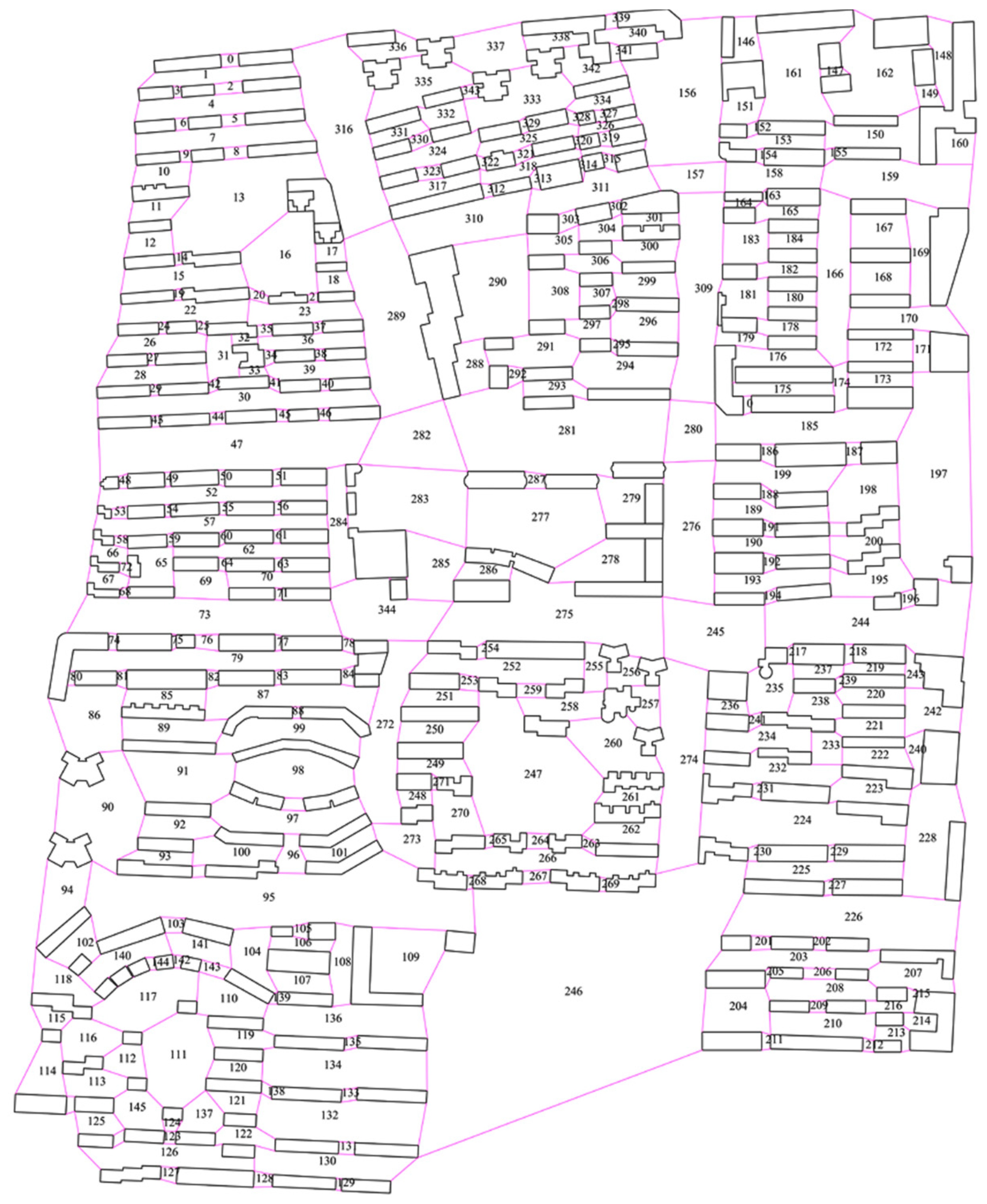
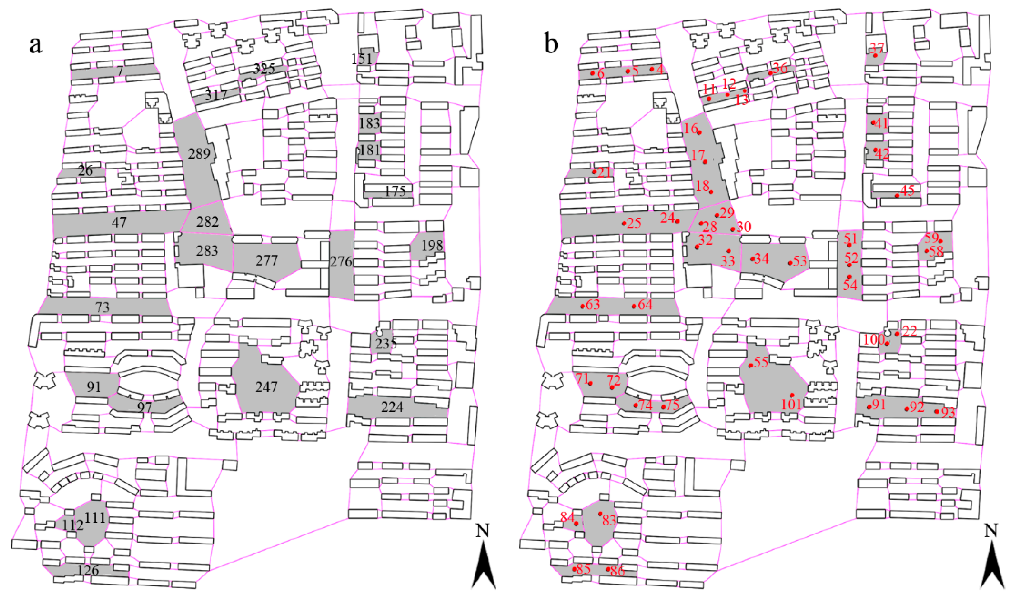
2.2. Spatial Partition and Quantification

The complexity of the chosen urban space not only increased the difficulty of determining the wind tunnel measurement points arrangement, but also led to the difficulty of the correlation analysis between spatial quantification and the PLW environment. Thus, it was necessary to divide the continuous space into identified subspaces. The method of space division, used in this study, is to connect the nearest convex angles of the building walls. This method ensures a number of subspaces in the same urban area division are as low as possible, conforming to the operability, economy, and spatial cognitive principles [38,39]. According to the principle of connecting an adjacent building’s external corner, the study case was divided into 352 subspaces using pink partition lines. The subspaces are numbered, from 0 to 351 (Figure 6).

These subspaces can be quantified by the urban spatial quantitative method, so as to provide a foundation for correlation research. In correlation research, the spatial characteristics’ indices of an urban space should reflect the characteristics of the subspaces. Furthermore, the spatial characteristics’ indices should be reversible, for architecture and urban design. For these reasons, the spatial characteristics’ indices used in this study are “openness,” “area” and “shape” [38,39]. These spatial characteristics’ indices can be calculated by Equations (2) to (4).

$$\mathrm{Openness}=\frac{{\mathrm{N}}_{\mathrm{o}}\times {\mathrm{A}}_{\mathrm{O}}}{360}(-)$$

(2)

where openness (O) quantifies the openness of a subspace. ${\mathrm{N}}_{\mathrm{o}}$ is the number of openings in the space around the measurement point, and ${\mathrm{A}}_{\mathrm{O}}$ is the sum of the opening angles of the space around the measurement point.

$$\mathrm{Area}={{\displaystyle \sum }}^{\text{}}\frac{{\mathrm{r}}_{\mathrm{i}}{\mathrm{r}}_{\mathrm{i}+1}\sin 1°}{2},i\left(1,2,3,\cdots ,360\right)\left({\mathrm{m}}^2\right)$$

(3)

where area (A) quantifies the size of a subspace. $r_i$ is the length of the number i ray, from a measurement point to the boundary of the subspace, 1 ≤ i ≤ n. n is the number of rays emitted horizontally from the measuring point to the surroundings of the subspace.

$$\mathrm{Shape}=\frac{{\mathrm{r}}_{\mathrm{ave}}}{{\mathrm{r}}_{\max }}(-)$$

(4)

where shape (S) quantifies the narrowness of a subspace. ${\mathrm{r}}_{\mathrm{ave}}$ is the average length of the number n ray, and ${\mathrm{r}}_{\max }$ is the maximum length of the number n rays. The three urban spatial characteristics’ indices of the 352 subspaces were calculated, and the results are detailed in

Table 2. Spatial characteristic indices of 352 subspaces (… stands for ellipsis).

Subspace Number	Openness (O)/-	Area (A)/m2	Shape (S)/-
0	0.94	224	0.76
1	1.19	2242	0.24
2	0.89	314	0.61
3	0.63	88	0.72
…	…	…	…
351	1.43	265	0.65

. The complete quantization results of the 352 subspaces can be seen in Supplementary Material: Table S1.

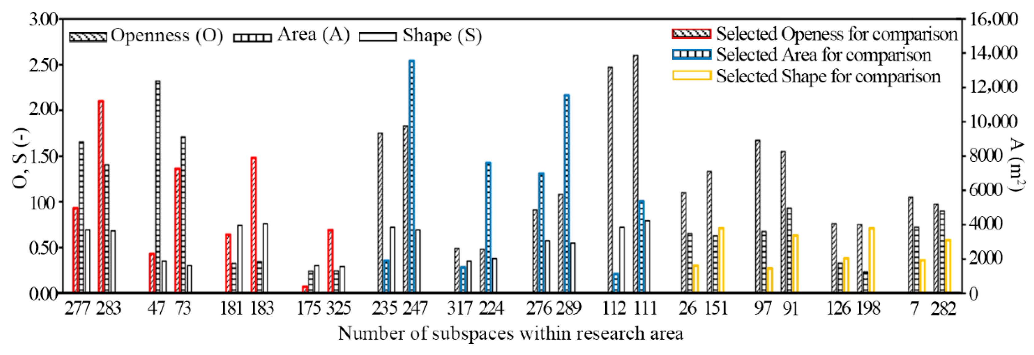
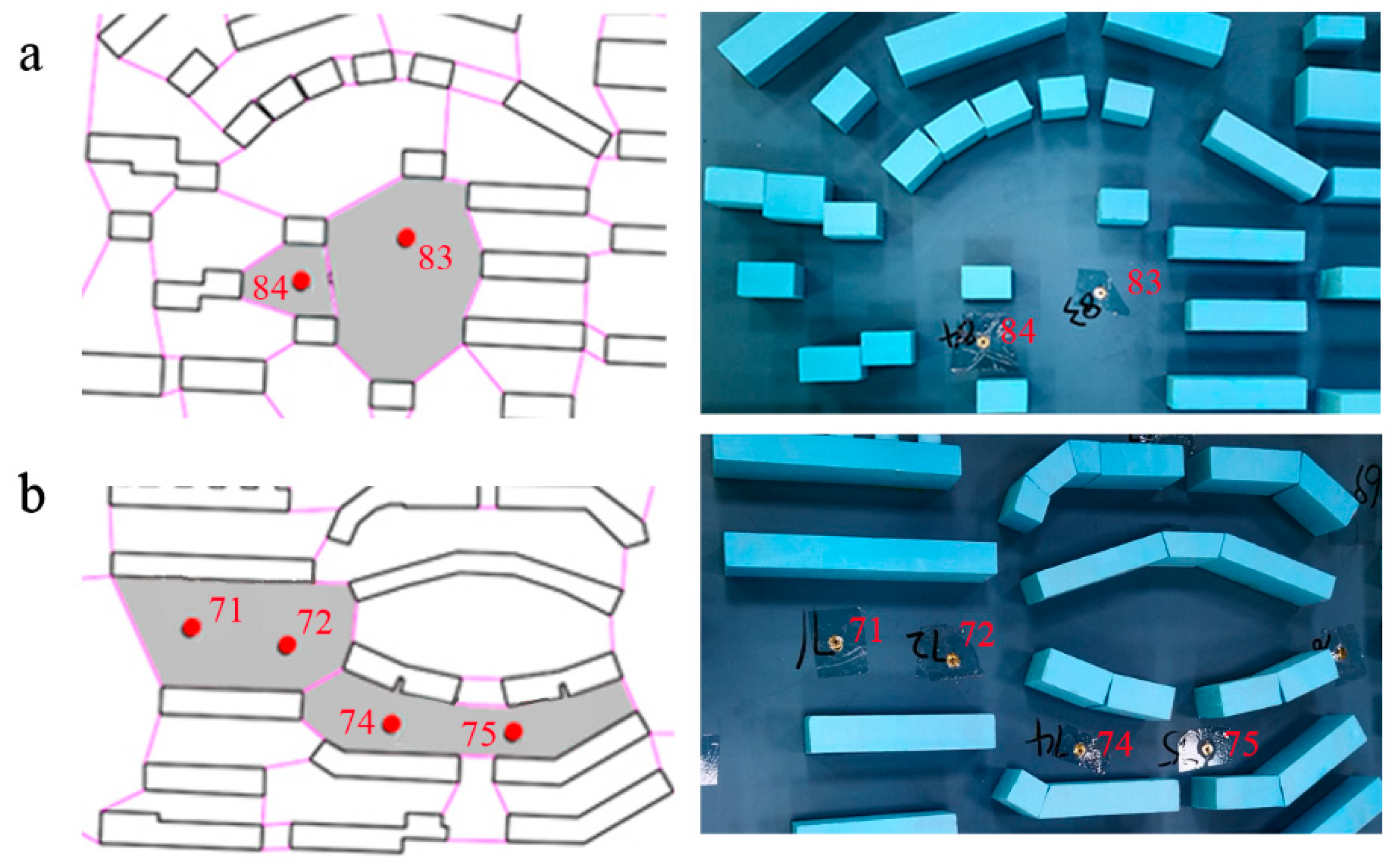
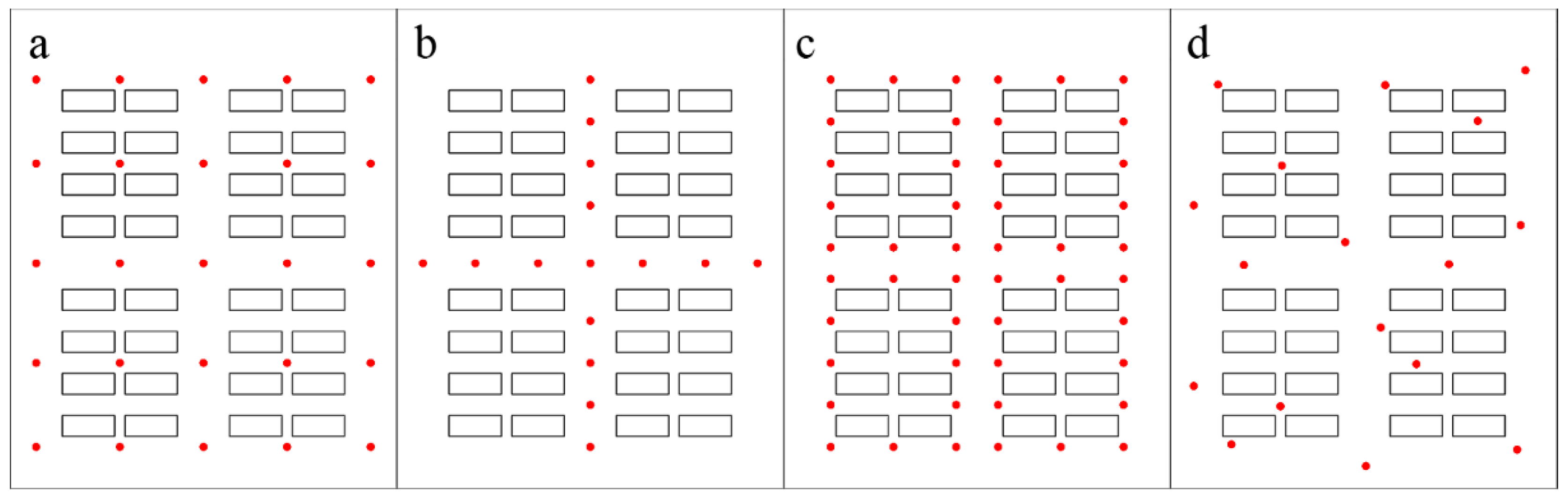
2.3. The Arrangement of Measurement Points

By comparing the indices, shown in Table 2, the pairs of subspaces with prominent urban spatial indices are selected as the key locations of the wind tunnel experiment. Since there are three spatial characteristics’ indices used in this study, the selection criterion was: “One index value of the two subspaces is quite different, but the other two index values are similar.” The subspaces were selected in pairs. The difference between the indices of each pair of subspaces was compared with the wind tunnel experimental results. The subspace that was too small for measurement points to be located in it was excluded first. The specific selection criteria were as follows:

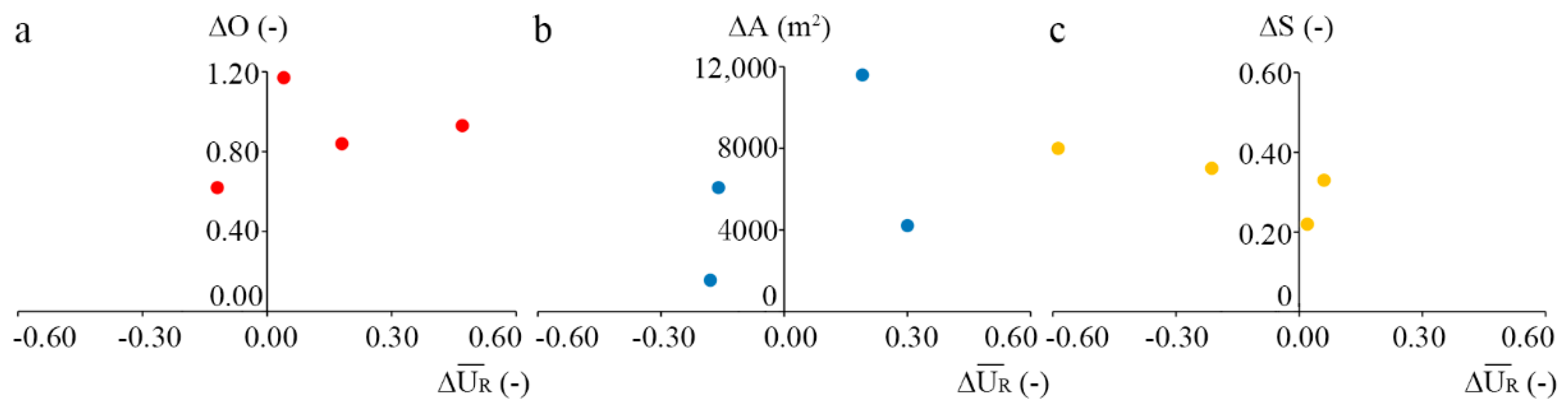
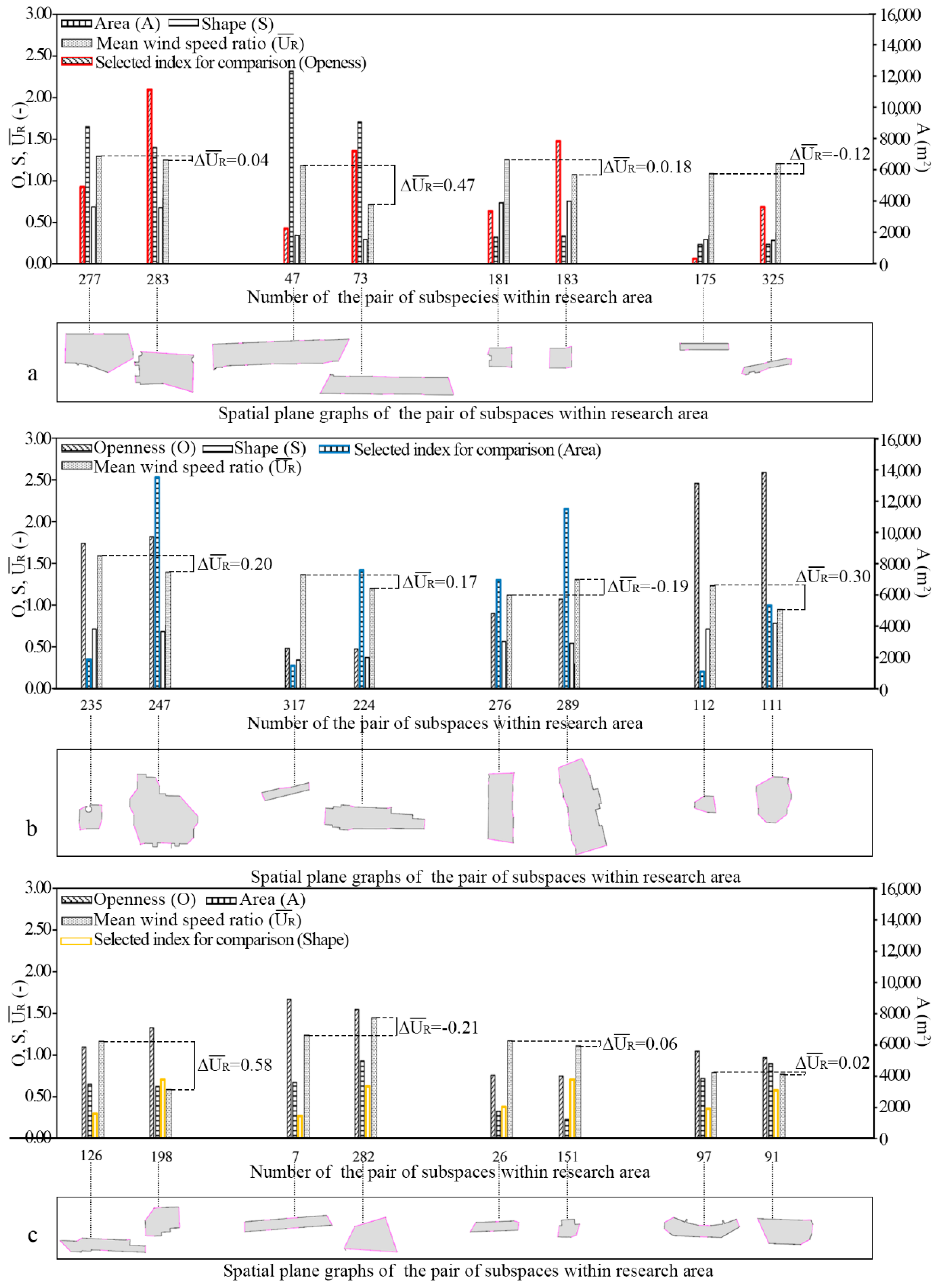
• Selected index for comparison (O): The openness is quite different for each pair of subspaces, but the area and shape are similar.
• Selected index for comparison (A): The area is quite different for each pair of subspaces, but the shape and openness are similar.
• Selected index for comparison (S): The shape is quite different for each pair of subspaces, but the openness and area are similar.

In the 352 subspaces, there were only 8 (4 pairs) subspaces satisfying selection criterion 3. The numbers of subspaces satisfying the selection criteria 1 and 2 were both more than 8 (4 pairs). In order to keep the number of subspaces consistent, all the numbers of subspaces under the three selection criteria were 8 (4 pairs). Except for when the number of subspaces is zero, there is no effect on the overall results by the number. According to the difference value of the openness of each pair of spaces (△O) from high to low, four pairs of subspaces were selected. According to the difference value of the area of each pair of spaces (△A) from high to low, four pairs of subspaces were selected. According to the difference value of the shape of each pair of spaces (△S) from high to low, four pairs of subspaces were selected. In accordance with the abovementioned selection criteria, 24 (12 pairs) subspaces are displayed in

Table 3. Spatial characteristic indices of 24 selected subspaces.

Selected Index for Comparison (Openness)					Selected Index for Comparison (Area)					Selected Index for Comparison (Shape)
Subspace Number	O	A	S	△O	Subspace Number	O	A	S	△A	Subspace Number	O	A	S	△S
	(-)	(m2)	(-)	(-)		(-)	(m2)	(-)	(m2)		(-)	(m2)	(-)	(-)
277	0.93	8810	0.69	1.17	235	1.75	1911	0.72	11,594	277	126	1.10	3481	0.41
283	2.10	7467	0.68		247	1.83	13,505	0.69		283	198	1.33	3338
47	0.43	12,330	0.35	0.93	317	0.49	1516	0.35	6075	47	7	1.67	3598	0.36
73	1.36	9094	0.3		224	0.48	7591	0.38		73	282	1.55	4972
181	0.64	1754	0.74	0.84	276	0.91	6968	0.57	4534	181	26	0.76	1763	0.33
183	1.48	1836	0.76		289	1.08	11,502	0.55		183	151	0.75	1241
175	0.07	1290	0.3	0.62	112	2.47	1136	0.72	4211	175	97	1.05	3846	0.22
325	0.69	1306	0.29		111	2.60	5347	0.79		325	91	0.97	4791

. A comparison diagram of the spatial characteristics’ indices of 24 (12 pairs) subspaces is shown in Figure 7.

Taking the 24 (12 pair) subspaces as the wind tunnel experiment’s key locations, can make up for the shortcomings of the arrangement of the measurement points. This method reduces the number of measurement points and avoids interference between the experimental probes. Placing measurement points using the perspective of the urban spatial characteristics, makes it easy to analyze the experimental results with respect to correlations. This method meets the requirements of correlation research on designated spaces, and solves the problems relating to spatial representativeness. The positions of the 24 subspaces in the total plane are shown in the gray filling of Figure 8a. About 1 to 3 measurement points are located in each subspace, and the number of measurement points is determined by the size of the area. There were 45 measurement points in the 24 subspaces. The wind tunnel measurement point locations are shown as the red dots in Figure 8b. Photos of the Irwin probes that were located on the model are shown in Figure 9.

3. Results and Discussion

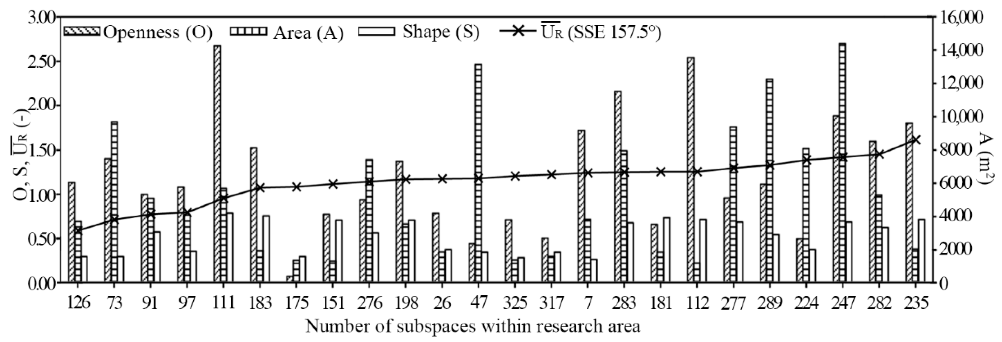
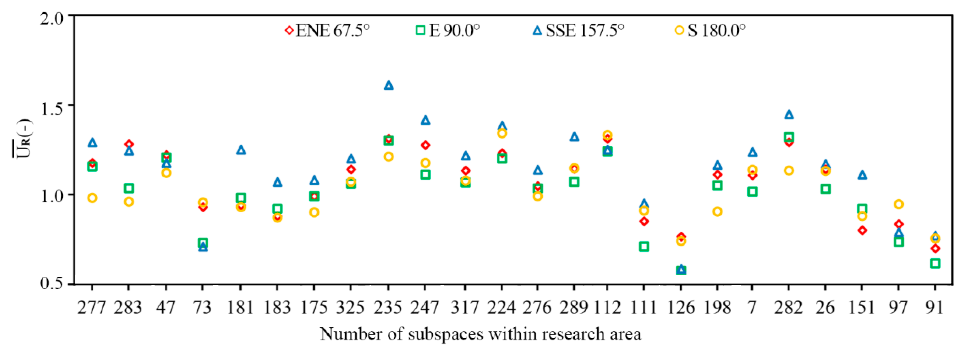
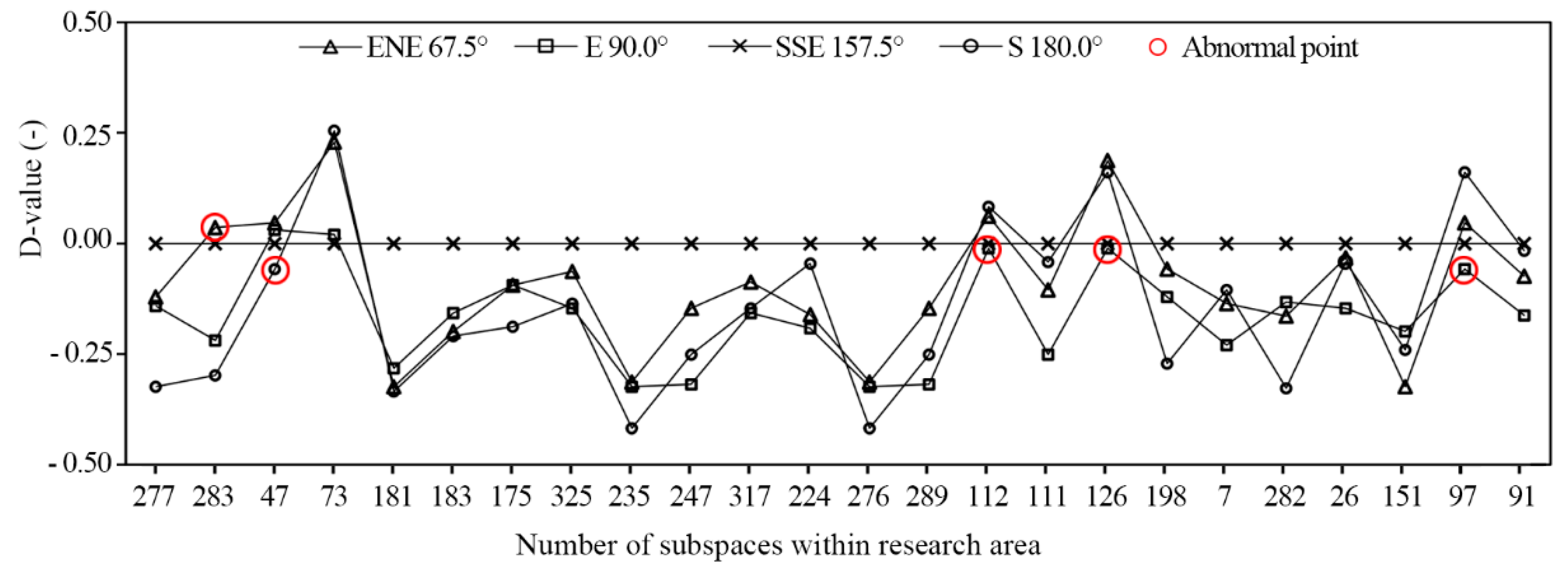
3.1. Mean Wind Velocity Ratio of the Subspaces in Different Wind Directions

Under eight experimental conditions (Case1 to Case 8 shown in Table 1) the values of mean wind velocity were measured at 45 measurement points, illustrated in

Table 4. Mean wind velocity experimental results (m/s) (… stands for ellipsis).

Measurement Points Number	Experimental Conditions
	Case 1	Case 2	Case 3	Case 4	Case 5	Case 6	Case 7	Case 8
34	2.69	3.20	2.91	2.75	2.32	4.26	3.50	3.66
53	2.58	3.22	2.38	2.90	2.77	4.38	2.45	3.55
32	1.99	2.36	2.29	2.71	2.08	2.78	2.44	3.40
…	…	…	…	…	…	…	…	…
59	2.26	2.42	3.13	2.87	2.04	2.80	2.51	3.49

. The complete experimental results can be seen in the Supplementary Material: Table S2.

The wind velocity values at each measurement point, obtained under a certain experimental wind velocity, are of little significance in practical applications [40,41,42]. The wind velocity ratio (${\mathrm{U}}_{\mathrm{R}}$) can be used instead to evaluate the wind environment [36,43]. ${\mathrm{U}}_{\mathrm{R}}$ is used to reflect the degree of wind velocity change in the 24 (12 pairs) selected subspaces and is calculated by Equation (5):

$${\mathrm{U}}_{\mathrm{R}}=\frac{{\mathrm{V}}_{\mathrm{r}}}{{\mathrm{V}}_0}(-)$$

(5)

where ${\mathrm{V}}_{\mathrm{r}}$ is the wind velocity measured at the probe height at each measurement point, and ${\mathrm{V}}_0$ is the incoming wind velocity at the probe height [36,43].

After calculating the ${\mathrm{U}}_{\mathrm{R}}$ at the 45 measurement points by Equation (5), the calculation results were illustrated (Supplementary Material: Table S3). The average value of the two groups’ data under different wind velocity conditions was taken as the final wind velocity ratio at the 45 measurement points. Because of the different sizes of the 24 (12 pairs) selected subspaces, the number of measurement points arranged in each subspace varied from 1 to 3. The mean wind velocity ratio ($\overline{{\mathrm{U}}_{\mathrm{R}}}$) of each subspace is defined as the average value of the ${\mathrm{U}}_{\mathrm{R}}$ at all the measurement points in each subspace. The mean wind velocity ratios of the subspaces are shown in

Table 5. Mean wind velocity ratio ($\overline{{\mathrm{U}}_{\mathrm{R}}}$) calculation results (… stands for ellipsis).

Subspace Number	Measurement Points Number	$\mathbf{Wind}\mathbf{Velocity}\mathbf{Ratio},{\mathbf{U}}_{\mathbf{R}}(-)$				$\mathbf{Mean}\mathbf{Wind}\mathbf{Velocity}\mathbf{Ratio},\overline{{\mathbf{U}}_{\mathbf{R}}}(-)$
		S	SSE	E	ENE	S	SSE	E	ENE
		180.0°	157.5°	90.0°	67.5°	180°	157.5°	90.0°	67.5°
277	34	1.06	1.52	1.32	1.31	0.98	1.29	1.16	1.18
	53	0.90	1.06	0.99	1.04
283	32	0.85	1.06	0.98	1.25	0.96	1.25	1.04	1.28
	33	1.07	1.43	1.09	1.31
…	…	…	…	…	…	…	…	…	…
91	71	0.68	0.9	0.64	0.77	0.76	0.77	0.62	0.70
	72	0.83	0.64	0.59	0.63

. The complete values of the mean wind velocity ratio ($\overline{{\mathrm{U}}_{\mathrm{R}}}$) can be seen in the Supplementary Material: Table S4.

The scatter diagrams of $\overline{{\mathrm{U}}_{\mathrm{R}}}$ values of 24 (12pairs) subspaces under the four experimental wind directions are illustrated in Figure 10. To better understand the correlation between $\overline{{\mathrm{U}}_{\mathrm{R}}}$ and wind direction, the correlation coefficients of $\overline{{\mathrm{U}}_{\mathrm{R}}}$ values under four wind directions were calculated, which are shown in

Table 6. Correlation coefficients of $\overline{{\mathrm{U}}_{\mathrm{R}}}$ under four wind directions.

Wind Direction	ENE 67.5°	E 90.0°	SSE 157.5°	S 180.0°
ENE 67.5°	1.00
E 90.0°	0.91	1.00
SSE 157.5°	0.83	0.92	1.00
S 180.0°	0.85	0.81	0.75	1.00

. The correlation coefficients of $\overline{{\mathrm{U}}_{\mathrm{R}}}$ values between four wind directions are from 0.75 to 0.92. Correlation coefficients display the changes of $\overline{{\mathrm{U}}_{\mathrm{R}}}$ values of 24 (12pairs) subspaces under the four experimental wind directions; they are close. The $\overline{{\mathrm{U}}_{\mathrm{R}}}$s of the subspaces are not significantly affected by the wind direction. For the same wind direction, the $\overline{{\mathrm{U}}_{\mathrm{R}}}$ of different subspaces are very different, which indirectly indicates that there is a correlation between the $\overline{{\mathrm{U}}_{\mathrm{R}}}$ and the urban spatial characteristics of the subspaces. In order to assess the changes of $\overline{{\mathrm{U}}_{\mathrm{R}}}$ values in 24 (12pairs) subspaces, the $\overline{{\mathrm{U}}_{\mathrm{R}}}$ values were analyzed further, as Figure 11 presents. Because the predominant wind direction in summer in Nanjing is SSE 157.5°, the $\overline{{\mathrm{U}}_R}$ of SSE 157.5° wind direction is defined as the normalized $\overline{{\mathrm{U}}_{\mathrm{R}}}$. The difference values (D-value) of $\overline{{\mathrm{U}}_{\mathrm{R}}}$ between the other three wind directions and SSE 157.5° wind direction were calculated. By comparing D-values of four wind directions, the abnormal points that affected the correlation coefficients can be found. The comparison results are shown in Figure 11; five abnormal points were found, which are marked by red circles. They are $\overline{{\mathrm{U}}_{\mathrm{R}}}$ of number 283 under NEN 67.5°, $\overline{{\mathrm{U}}_{\mathrm{R}}}$ of number 47 under S 180.0°, $\overline{{\mathrm{U}}_{\mathrm{R}}}$ of number 112 under E 90.0°, $\overline{{\mathrm{U}}_{\mathrm{R}}}$ of number 126 under E 90.0°, and $\overline{{\mathrm{U}}_{\mathrm{R}}}$ of number 97 under E 90.0°. This result may have been due to the deficiency of space partition method or the deficiency of the average calculation of wind velocity ratios in subspace.

3.2. Correlation between Wind Velocity Ratio and Urban Space Quantification

According to the results shown in Section 3.1, the changes of $\overline{{\mathrm{U}}_{\mathrm{R}}}$ values of 24 subspaces under the four experimental wind directions were close. The $\overline{{\mathrm{U}}_{\mathrm{R}}}$ of the one wind direction can be considered to be representative for discussion. The $\overline{{\mathrm{U}}_{\mathrm{R}}}$ of SSE was chosen to be representative to discuss the correlation between the $\overline{{\mathrm{U}}_{\mathrm{R}}}$ and urban spatial characteristics’ indices. The $\overline{{\mathrm{U}}_{\mathrm{R}}}$ of the 24 subspaces in the SSE 157.5° wind direction were arranged in ascending order and superposed on the spatial characteristics’ indices in Figure 12. The specific correlation between the spatial characteristics’ indices and $\overline{{\mathrm{U}}_{\mathrm{R}}}$ was hard to find, as the graph clearly shows. None of the histograms of the spatial characteristics’ indices showed a significant correlation with the $\overline{{\mathrm{U}}_{\mathrm{R}}}$ of SSE 157.5°. The correlation between $\overline{{\mathrm{U}}_{\mathrm{R}}}$ and spatial characteristics’ indices could be directly analyzed in this way.

Reviewing the selection criteria of the 24 (12 pairs) subspaces within the research area in Section 2.3, the spatial characteristics’ indices of 12 pairs according to the following rule: one index value of the two subspaces is quite different, but the other two index values are similar. The 24 (12 pairs) subspaces were divided into three groups according to △O, △A, and △S. The difference value (△$\overline{{\mathrm{U}}_{\mathrm{R}}}$) of the mean wind speed ratio of each pair of subspaces’ was calculated, as illustrated in

Table 7. Calculation of the value of the mean wind velocity ratio’s ($\overline{{\mathrm{U}}_{\mathrm{R}}}$) difference between the 12 pairs of subspaces.

Subspace Number	$\overline{{\mathbf{U}}_{\mathbf{R}}}(-)$	$△\overline{{\mathbf{U}}_{\mathbf{R}}}(-)$	Subspace Number	$\overline{{\mathbf{U}}_{\mathbf{R}}}(-)$	$△\overline{{\mathbf{U}}_{\mathbf{R}}}(-)$	Subspace Number	$\overline{{\mathbf{U}}_{\mathbf{R}}}(-)$	$△\overline{{\mathbf{U}}_{\mathbf{R}}}(-)$
277	1.29	–0.04	235	1.61	–0.19	126	0.59	0.58
283	1.25		247	1.42		198	1.17
47	1.18	–0.47	317	1.22	0.16	7	1.24	0.21
73	0.71		224	1.38		282	1.45
181	1.25	–0.18	276	1.14	0.18	26	1.17	–0.06
183	1.07		289	1.32		151	1.11
175	1.08	0.12	112	1.25	–0.30	97	0.79	–0.02
325	1.20		111	0.95		91	0.77

. The calculations of △$\overline{{\mathrm{U}}_{\mathrm{R}}}$ were compared with the spatial indicators’ characteristics again. The comparative results are illustrated in Figure 13.

One pair of subspaces includes number 277 and number 283; another pair of subspaces includes number 47 and number 73, and yet another pair of subspaces includes number 181 and number 183. The △$\overline{{\mathrm{U}}_{\mathrm{R}}}$s of pairs of subspaces are –0.04, –0.47, and –0.18, whereas the △Os are 1.17, 0.93, and 0.84 (Figure 13a). By comparison, their area and shape index values are similar, but their openness index values are quite different. Without considering the location and surrounding influence of the subspaces in the research area, it can perhaps be inferred that, when two subspaces have similar openness and area index values, but differently shaped index values, a lower openness index value may lead to a higher $\overline{{\mathrm{U}}_{\mathrm{R}}}$. The $\overline{{\mathrm{U}}_{\mathrm{R}}}$ and openness presents a negative correlation. When the pair of subspaces includes number 175 and number 325, their △$\overline{{\mathrm{U}}_{\mathrm{R}}}$ is 0.12, whereas their △O is 0.62. Their △$\overline{{\mathrm{U}}_{\mathrm{R}}}$ and △O present a different rule to that of the other pairs of subspaces shown in Figure 14a, but their lower openness index value may lead to a lower $\overline{{\mathrm{U}}_{\mathrm{R}}}$. This result may be due to the influence of the method of space division. The next pair of subspaces includes number 235 and number 247, and the other pair of subspaces includes number 112 and number 111; the △$\overline{{\mathrm{U}}_{\mathrm{R}}}\mathrm{s}$ of the pairs of subspaces are –0.19 and –0.30, whereas their △As are 11594 and 4211 (Figure 13b). By comparison, their openness and shape index values are similar, but their area index values are quite different. Without considering the location and surrounding influence of the subspaces in the research area, it can perhaps be inferred that, when two subspaces have similar openness and shape index values, but different area index values. A lower area index value may lead to a higher $\overline{{\mathrm{U}}_{\mathrm{R}}}$. The next pair of subspaces includes number 317 and number 224, and the other pair of subspaces includes number 276 and number 289; their △$\overline{{\mathrm{U}}_{\mathrm{R}}}$s are 0.16 and 0.18, whereas their △As are 6075 and 4534. Their △$\overline{{\mathrm{U}}_{\mathrm{R}}}$ and △A present a different rule to those of the other pairs of subspaces shown in Figure 14b, but their lower area index value may lead to a lower $\overline{{\mathrm{U}}_{\mathrm{R}}}$. The △$\overline{{\mathrm{U}}_{\mathrm{R}}}$ and △A present no clear correlation. This result may be due to the influence of the method of spatial partition or the deficiency of the average calculation of wind velocity ratios in subspace. The next pair of subspaces includes number 126 and number 198, and another pair of subspaces includes number 7 and number 282; the △$\overline{{\mathrm{U}}_{\mathrm{R}}}\mathrm{s}$of the pairs of subspaces are 0.58 and 0.21, whereas their △Ss are 0.41 and 0.36 (Figure 13c). By comparison, their openness and area index values are similar, but their shape index values are quite different. Without considering the location and surrounding influence of the subspaces in the research area, it can perhaps be inferred that, when two subspaces have similar openness and area index values, but different shape index values, a higher shape index value may lead to a higher $\overline{{\mathrm{U}}_{\mathrm{R}}}$. For the pair of subspaces including number 26 and number 151, and the pair of subspaces including number 97 and number 91, their △$\overline{{\mathrm{U}}_{\mathrm{R}}}$s are –0.06 and –0.02, whereas their △Ss are 0.33 and 0.22. Their △$\overline{{\mathrm{U}}_{\mathrm{R}}}$s and △Ss present a different rule to that of the other pairs of subspaces shown in Figure 14c, but their lower area index value may lead to a higher $\overline{{\mathrm{U}}_{\mathrm{R}}}$. The △$\overline{{\mathrm{U}}_{\mathrm{R}}}$ and △S present no obvious correlation. This result may be due to the influence of the method of spatial partition or the deficiency of the calculation of average wind velocity ratios in the subspace.

4. Conclusions

A typical urban area in Nanjing, China was selected as the research object in this study. Through an analysis of urban space quantification and pedestrian-level ventilation, the present findings suggested a method for correlation research on the correlation between the PLW environment and an urban space. The following conclusions have been drawn:

In correlation research, the arrangement of measurement points in wind tunnel experiments can be determined in accordance with urban spatial characteristics. An appropriate space needs to be found first, then points need to be located. Using the method of space division, that is, to connect the nearest convex angles of the building walls, a complex urban space is divided into ordered subspaces. After quantization of subspaces, the pairs of subspaces with prominent urban spatial indices should be selected as the key locations of wind tunnel experiment. This method can improve the efficiency of wind tunnel experiments and reduce the cost of the experiments. It also provides support for a preliminary analysis of the correlation between urban space and the PLW environment.

In the case investigated, under the same experimental conditions, the correlation coefficients of $\overline{{\mathrm{U}}_{\mathrm{R}}}$ values under the ENE 67.5°, E 90.0°, SSE 157.5°, and S 180.0° wind directions were high. Correlation coefficients showed that the changes of the $\overline{{\mathrm{U}}_{\mathrm{R}}}$ values of 24 (12pairs) subspaces under the four experimental wind directions were close. The $\overline{{\mathrm{U}}_{\mathrm{R}}}$ values of the subspaces were not significantly affected by the wind direction.

When making the correlation analysis between mean wind speed ratio and spatial characteristics’ indices, the direct numerical comparison was not able to find a correlation. The correlation between $\overline{{\mathrm{U}}_{\mathrm{R}}}$ and spatial characteristics’ indices cannot be directly analyzed in this way. By comparing the difference values of mean wind speed and indices between each pair of subspaces, some correlations between $\overline{{\mathrm{U}}_{\mathrm{R}}}$ and spatial characteristics’ indices can be found. The $\overline{{\mathrm{U}}_{\mathrm{R}}}$ and openness of a subspace present a negative correlation. Limited by the spatial partition method, the correlation between $\overline{{\mathrm{U}}_{\mathrm{R}}}$ and the other indices is not obvious.

Wind velocity within an urban environment strongly changes from one point to another, even in small spaces. Due to the limitations of wind tunnel test conditions, the number of measurement points in subspaces should not be too large. For this study, the mean wind velocity ratio was obtained with not more than three measurement points; the average values of those measurements could not be representative of the actual wind environment in the subspace. This deficiency can be remedied by extracting more data from CFD in the future study. The correlation analysis between the spatial characteristics’ indices and $\overline{{\mathrm{U}}_{\mathrm{R}}}$ did not consider the location and surrounding influence of the subspaces in the research area. However, it is well known that these are important factors which affect wind environment. This study selected and discussed three spatial characteristics’ indices of urban spaces, but the weight of the three indices and their mechanistic impacts on the PLW environment were not discussed. In a future study, we will design standard models to analyze the specific impact of urban spatial characteristics’ indices on PLW environment. The spatial division method should also be corrected from the perspective of wind environment, based on the present findings.

This article is a first attempt towards a correlation study. The urban spatial characteristics’ indices need to be further improved, and future studies will take into account the height index and other important indices to form a more complete urban spatial-characteristic index system.

References

1. Oke, T.R. Towards a prescription for the greater use of climatic principles in settlement planning. Energy Build. 1984, 7, 1–10. [Google Scholar] [CrossRef]
2. Oke, T.R. Street design and urban canopy layer climate. Energy Build. 1988, 11, 103–113. [Google Scholar] [CrossRef]
3. Gabel, J. The Skyscraper Surge Continues in 2015, The ‘Year of 100 Supertalls’. In CTBUH Year in Review: Tall Trends of 2015, and Forecasts for 2016; The Council on Tall Buildings and Urban Habitat: Chicago, IL, USA, 2015. [Google Scholar]
4. Krüger, E.L.; Minella, F.O.; Rasia, F. Impact of urban geometry on outdoor thermal comfort and air quality from field measurements in Curitiba, Brazil. Build. Environ. 2011, 46, 621–634. [Google Scholar] [CrossRef]
5. Grant, R.H.; Heisler, G.M.; Herrington, L.P. Full-scale comparison of a wind-tunnel simulation of windy locations in an urban area. J. Wind Eng. Ind. Aerodyn. 1988, 31, 335–341. [Google Scholar] [CrossRef]
6. Arens, EA. Designing for an acceptable wind environment. Transp. Eng. J. 1981, 107, 127–141. [Google Scholar]
7. Adamek, K.; Vasan, N.; Elshaer, A.; English, E.; Bitsuamlak, G. Pedestrian level wind assessment through city development: A study of the financial district in Toronto. Sustain. Cities Soc. 2017, 35, 178–190. [Google Scholar] [CrossRef]
8. Hang, J.; Sandberg, M.; Li, Y. Effect of urban morphology on wind condition in idealized city models. Atmos. Environ. 2009, 43, 869–878. [Google Scholar] [CrossRef]
9. Ng, E. Policies and technical guidelines for urban planning of high-density cities–air ventilation assessment (AVA) of Hong Kong. Build. Environ. 2009, 44, 1478–1488. [Google Scholar] [CrossRef]
10. Blocken, B.; Carmeliet, J. Pedestrian wind environment around buildings: Literature review and practical examples. J. Therm. Envel. Build. Sci. 2004, 28, 107–159. [Google Scholar] [CrossRef]
11. Blocken, B.; Stathopoulos, T.; Van Beeck, J. Pedestrian-level wind conditions around buildings: Review of wind-tunnel and CFD techniques and their accuracy for wind comfort assessment. Build. Environ. 2016, 100, 50–81. [Google Scholar] [CrossRef]
12. Iqbal, Q.M.Z.; Chan, A.L.S. Pedestrian level wind environment assessment around group of high-rise cross-shaped buildings: Effect of building shape, separation and orientation. Build. Environ. 2016, 101, 45–63. [Google Scholar] [CrossRef]
13. Mittal, H.; Sharma, A.; Gairola, A. A review on the study of urban wind at the pedestrian level around buildings. J. Build. Eng. 2018, 18, 154–163. [Google Scholar] [CrossRef]
14. Blocken, B.; van Druenen, T.; Toparlar, Y.; Malizia, F.; Mannion, P.; Andrianne, T.; Marchal, T.; Maas, G.-J.; Diepens, J. Aerodynamic drag in cycling pelotons: New insights by CFD simulation and wind tunnel testing. J. Wind Eng. Ind. Aerodyn. 2018, 179, 319–337. [Google Scholar] [CrossRef]
15. Wise, A.F.E.; Sexton, D.E.; Lillywhite, M.S.T. Studies of Air Flow Round Buildings (No. Design Ser-38); Building Research Station: Watford, UK, 1965. [Google Scholar]
16. Lawson, T.V. The Wind Environment of Buildings: A Logical Approach to the Establishment of Criteria; Report No. TVL.; Department of Aeronautical Engineering, University of Bristol: Bristol, UK, 1973; p. 7321. [Google Scholar]
17. Wu, H.; Stathopoulos, T. Wind-tunnel techniques for assessment of pedestrian-level winds. J. Eng. Mech. 1993, 119, 1920–1936. [Google Scholar] [CrossRef]
18. Yassin, M.F.; Kato, S.; Ooka, R.; Takahashi, T.; Kouno, R. Field and wind-tunnel study of pollutant dispersion in a built-up area under various meteorological conditions. J. Wind Eng. Ind. Aerodyn. 2005, 93, 361–382. [Google Scholar] [CrossRef]
19. Kubota, T.; Miura, M.; Tominaga, Y.; Mochida, A. Wind tunnel tests on the relationship between building density and pedestrian-level wind velocity: Development of guidelines for realizing acceptable wind environment in residential neighborhoods. Build. Environ. 2008, 43, 1699–1708. [Google Scholar] [CrossRef]
20. Antoniou, N.; Montazeri, H.; Wigo, H.; Neophytou, M.K.-A.; Blocken, B.; Sandberg, M. CFD and wind-tunnel analysis of outdoor ventilation in a real compact heterogeneous urban area: Evaluation using “air delay”. Build. Environ. 2017, 126, 355–372. [Google Scholar] [CrossRef]
21. He, Y.; Tablada, A.; Wong, N.H. A parametric study of angular road patterns on pedestrian ventilation in high-density urban areas. Build. Environ. 2019, 151, 251–267. [Google Scholar] [CrossRef]
22. Tominaga, Y.; Yoshie, R.; Mochida, A.; Kataoka, H.; Harimoto, K.; Nozu, T. Cross comparisons of CFD prediction for wind environment at pedestrian level around buildings. Part 2: Comparison of Results for Flowfield around Building Complex in Actual Urban Area. In Proceedings of the Sixth Asia-Pacific Conference on Wind Engeenering (APCWE-VI), Seoul, Korea, 12–14 September 2005; pp. 2661–2670. [Google Scholar]
23. Liu, X.P.; Niu, J.L.; Kwok, K.C.; Wang, J.H.; Li, B.Z. Investigation of indoor air pollutant dispersion and cross-contamination around a typical high-rise residential building: Wind tunnel tests. Build. Environ. 2010, 45, 1769–1778. [Google Scholar] [CrossRef]
24. Weerasuriya, A.U.; Tse, K.T.; Zhang, X.; Li, S.W. A wind tunnel study of effects of twisted wind flows on the pedestrian-level wind field in an urban environment. Build. Environ. 2018, 128, 225–235. [Google Scholar] [CrossRef]
25. An, K.; Fung, J.C.H.; Yim, S.H.L. Sensitivity of inflow boundary conditions on downstream wind and turbulence profiles through building obstacles using a CFD approach. J. Wind Eng. Ind. Aerodyn. 2013, 115, 137–149. [Google Scholar] [CrossRef]
26. Toparlar, Y.; Blocken, B.; Maiheu, B.; Van Heijst, G. A review on the CFD analysis of urban microclimate. Renew. Sustain. Energy Rev. 2017, 80, 1613–1640. [Google Scholar] [CrossRef]
27. Peng, Y.; Gao, Z.; Buccolieri, R.; Ding, W. An investigation of the quantitative correlation between urban morphology parameters and outdoor ventilation efficiency indices. Atmosphere 2019, 10, 33. [Google Scholar] [CrossRef]
28. You, W.; Shen, J.; Ding, W. Improving residential building arrangement design by assessing outdoor ventilation efficiency in different regional spaces. Archit. Sci. Rev. 2018, 61, 202–214. [Google Scholar] [CrossRef]
29. Gao, Y.; Yao, R.; Li, B.; Turkbeyler, E.; Luo, Q.; Short, A. Field studies on the effect of built forms on urban wind environments. Renew. Energy 2012, 46, 148–154. [Google Scholar] [CrossRef]
30. Gu, Y.; Ding, W. Reseach on the Setting of the Range of Test Area in CFD Simulation of City Slices. Master’s Thesis, Nanjing University, Nanjing, China, 2018. (In Chinese). [Google Scholar]
31. Tominaga, Y.; Yoshie, R.; Mochida, A.; Kataoka, H.; Harimoto, K.; Nozu, T. Cross comparisons of CFD prediction for wind environment at pedestrian level around buildings. Part 1: Comparison of Results for Flow-field around a High-rise Building Located in Surrounding City Blocks. In Proceedings of the Sixth Asia-Pacific Conference on Wind Engeenering (APCWE-VI), Seoul, Korea, 12–14 September 2005; pp. 2648–2659. [Google Scholar]
32. China Meteorological Information Center Meteorological. Chinese Building Thermal Environment Analysis of Specialized Meteorological Data Collection; China Architecture & Building Press: Beijing, China, 2005. (In Chinese) [Google Scholar]
33. Mattuella, J.M.L.; Loredo-Souza, A.M.; Oliveira, M.G.K.; Petry, A.P. Wind tunnel experimental analysis of a complex terrain micrositing. Renew. Sustain. Energy Rev. 2016, 54, 110–119. [Google Scholar] [CrossRef]
34. Irwin, H.P.A.H. A simple omnidirectional sensor for wind-tunnel studies of pedestrian-level winds. J. Wind Eng. Ind. Aerodyn. 1981, 7, 219–239. [Google Scholar] [CrossRef]
35. Li, Y. Study on Wind Tunnel Experiment and Its Application in the Field of Architectural Construction. Build. Sci. 2011, 27, 117–122. [Google Scholar]
36. Standard for Wind Tunnel Test of Buildings and Structures (JGJ/T 338-2014); China Architecture & Building Press: Beijing, China, 2014. (In Chinese)
37. Load Code for the Design of Building Structures (GB 50009-2012). China Architecture & Building Press: Beijing, China, 2012; pp. 31–32. (In Chinese)
38. Ji, H.; Peng, Y.; Ding, W. A Quantitative Study of Geometric Characteristics of Urban Space Based on the Correlation with Microclimate. Sustainability 2019, 11, 4951. [Google Scholar] [CrossRef]
39. Ji, H.; Ding, W.; Tang, L. A Classification Method and System of Urban Street Spatial Form. China Patent 201910379538.0, 8 May 2019. (In Chinese). [Google Scholar]
40. Bu, Z.; Kato, S.; Ishida, Y.; Huang, H. New criteria for assessing local wind environment at pedestrian level based on exceedance probability analysis. Build. Environ. 2009, 44, 1501–1508. [Google Scholar] [CrossRef]
41. Bady, M.; Kato, S.; Ishida, Y.; Huang, H.; Takahashi, T. Application of exceedance probability based on wind kinetic energy to evaluate the pedestrian level wind in dense urban areas. Build. Environ. 2011, 46, 1834–1842. [Google Scholar] [CrossRef]
42. Willemsen, E.; Wisse, J.A. Design for wind comfort in The Netherlands: Procedures, criteria and open research issues. J. Wind Eng. Ind. Aerodyn. 2007, 95, 1541–1550. [Google Scholar] [CrossRef]
43. Hu, T.; Yoshie, R. Indices to evaluate ventilation efficiency in newly-built urban area at pedestrian level. J. Wind Eng. Ind. Aerodyn. 2013, 112, 39–51. [Google Scholar] [CrossRef]
Figure 1. Four main arrangements of the wind tunnel measurement points. Display of (a) the arrays arrangement, (b) along streets arrangement, (c) around buildings arrangement, and (d) the distributed arrangement. Red dots represent the measurement points.
Atmosphere 10 00564 g001
Figure 2. (a) Research area location from Google maps. (b) Research area plan.
Atmosphere 10 00564 g002
Figure 3. Schematic of the blocking rate ( η ) calculation. (a) The maximum vertical cross-sectional area ( A b ) of the study object. (b) η calculation schematic.
Atmosphere 10 00564 g003
Figure 4. (a) Wind tunnel plane diagram. (b) Photo of the model in the wind tunnel.
Atmosphere 10 00564 g004
Figure 5. (a) Vertical profile of the mean velocity. (b) Vertical profile of the turbulence intensity in the simulated boundary layer.
Atmosphere 10 00564 g005
Figure 6. Spatial partition diagram of the study object. The black numbers are subspace numbers, the black lines are building boundaries, and the pink lines are spatial partition lines.
Atmosphere 10 00564 g006
Figure 7. Diagram of the selected indices for comparison.
Atmosphere 10 00564 g007
Figure 8. (a) The positions of the 24 subspaces. Black numbers are subspace numbers. (b) Measurement points located in accordance with the urban spatial characteristics. Red dots are the positions of the measurement points, and red numbers are the measurement point numbers.
Atmosphere 10 00564 g008
Figure 9. (a) Number 83 and number 84 Irwin probes located on the model. (b) Number 71, number 72, number 74, and number 75 Irwin probes located on the model.
Atmosphere 10 00564 g009
Figure 10. Mean wind velocity ratio ( U R ¯ ) scatter diagram of 24 subspaces.
Atmosphere 10 00564 g010
Figure 11. Difference values (D-values) of U R ¯ between the other three wind directions and SSE 157.5°.
Atmosphere 10 00564 g011
Figure 12. U R ¯ of the SSE 157.5° wind direction and the spatial characteristics’ indices of 24 subspaces.
Atmosphere 10 00564 g012
Figure 13. Scatter diagrams of the difference value of spatial characteristics’ indices(△O, △A, △S) and the difference value of the mean wind speed ratio (△ U R ¯ ).
Atmosphere 10 00564 g013
Figure 14. Spatial characteristic indices of 12 pairs of spaces, compared with the difference value (△ U R ¯ ) of the mean wind speed ratio. (a) △O compared with △ U R ¯ ; (b) △A compared with △ U R ¯ ;(c) △S compared with △ U R ¯ .
Atmosphere 10 00564 g014