Next Article in Journal
ChromoCheck: Predicting Postnatal Chromosomal Trisomy Cases Using a Support Vector Machine Learning Model
Previous Article in Journal
Swertianin Suppresses M1 Macrophage Polarization and Inflammation in Metabolic Dysfunction-Associated Fatty Liver Disease via PPARG Activation
 
 
Due to scheduled maintenance work on our database systems, there may be short service disruptions on this website between 10:00 and 11:00 CEST on June 14th.
Article

Genetic Variation and Metapopulation Structure Inform Recovery Goals in a Threatened Species

by
Molly J. Garrett
1,†,
Courtney J. Conway
2,
Lisette P. Waits
1 and
Paul A. Hohenlohe
3,*
1
Department of Fish and Wildlife Sciences, College of Natural Resources, University of Idaho, Moscow, ID 83844, USA
2
U.S. Geological Survey, Idaho Cooperative Fish & Wildlife Research Unit, University of Idaho, Moscow, ID 83844, USA
3
Department of Biological Sciences, College of Science, University of Idaho, Moscow, ID 83844, USA
*
Author to whom correspondence should be addressed.
Current address: Hawai‘i Cooperative Studies Unit, University of Hawai‘i at Hilo, Hilo, HI 96720, USA.
Genes 2025, 16(6), 694; https://doi.org/10.3390/genes16060694
Submission received: 27 April 2025 / Revised: 17 May 2025 / Accepted: 22 May 2025 / Published: 8 June 2025
(This article belongs to the Special Issue Advances of Genetics in Wildlife Conservation and Management)

Abstract

:
Background: Monitoring genetic parameters is important for setting effective conservation and management strategies, particularly for small, fragmented, and isolated populations. Small, isolated populations face increased rates of genetic drift and inbreeding, which increase extinction risk especially when gene flow is limited. Methods: Here, we applied a Genotyping-in-Thousands by sequencing (GT-seq) panel to inform recovery action for the federally threatened northern Idaho ground squirrel (Urocitellus brunneus). We evaluated genetic diversity, structure, connectivity, and effective population size to address species recovery goals. Results: We delineated three types of conservation units: (1) three evolutionarily significant units that represent long-term population structure and variation, (2) nine management units that reflect current demographic connectivity and restrictions to gene flow, and (3) three adaptive units that capture adaptive differentiation across the species range. Effective population sizes per management unit were small overall (mean 38.16, range 2.3–220.9), indicating that recovery goals of 10 subpopulations with Ne > 500 have not been reached. Conclusions: Our results support the maintenance of connectivity within evolutionarily significant units through the restoration of dispersal corridors. Next steps could include further sampling of some subpopulations with low sample sizes, unsampled subpopulations, and subpopulations that are geographically isolated. Genotyping future samples with the same GT-seq panel would help to detect dispersal, assess effective population size, monitor the effects of inbreeding, and evaluate adaptive differentiation to monitor the effects of management action and environmental change.

1. Introduction

Understanding how environmental factors influence demography, connectivity, local adaptation, and ultimately resilience of small populations is critical to set conservation strategies and implement effective habitat management plans [1,2]. For example, increased levels of connectivity can facilitate gene flow between small populations that otherwise are vulnerable to high levels of genetic drift, while high levels of connectivity can also create genetically homogenous populations that may lack locally adapted phenotypes. Decreased connectivity may lead to inbreeding depression, where individuals suffer reduced fitness due to inbreeding [3,4]. Inbreeding depression can decrease the viability of small populations, especially in combination with underlying stochastic environmental, demographic, and genetic processes that are more pronounced in small populations [5,6]. Therefore, examining the underlying genetic factors is critical for effectively managing rare species.
An important metric for evaluating the relative importance of genetic factors for management and conservation is effective population size (Ne), which determines the expected rate of loss of genetic variation by genetic drift. Effective population size can also be used to estimate levels of inbreeding, which can affect fitness and viability of small populations [7]. Contemporary Ne estimates reflect evolutionary processes in one or a few recent generations and provide insight for conservation of populations facing ongoing threats [7]. Estimates of Ne can provide metrics for monitoring, goals for population recovery, and information to guide actions for threatened, fragmented, or small populations.
Determining Ne and other population genetic parameters is especially valuable for the conservation of species that exhibit a metapopulation structure. A metapopulation is an assemblage of interconnected breeding populations that occur in semi-independent subpopulations [8,9,10]. The interactions between genetic drift, gene flow, and local adaptation are variable between highly connected or isolated subpopulations. For example, small, isolated subpopulations can have relatively small Ne, a high degree of inbreeding, and high risk of local extinction [11,12]. On the other hand, metapopulations that are well connected can maintain genetic variation, with gene flow overcoming the loss of variation within subpopulations while still maintaining local adaptation [13,14]. As habitat fragmentation increases, monitoring gene flow and local adaptation within metapopulations is important for assessing population persistence for conservation and for designing management actions like genetic rescue or translocations.
Advancements in genomic sequencing technologies have provided increased resolution and aided the identification of adaptive loci, which have improved our ability to monitor and manage wildlife populations against the effects of environmental change and biodiversity loss [15,16]. Additionally, sequencing advances allow more neutral loci to be sequenced across the genome, which provides more accurate estimates of Ne and other metrics estimated with neutral loci (e.g., gene flow and connectivity). One such advance in amplicon sequencing is Genotyping-in-Thousands by sequencing (GT-seq) [17]. GT-seq targets a pre-identified set of genetic loci that are informative for a specific suite of objectives, and many samples can be genotyped to monitor genetic change over time and/or space. In addition to its relative low costs, GT-seq can be applied to lower-quality DNA samples relative to some other genomic techniques, so it is applicable to minimally invasive sampling in rare or threatened populations [18,19,20]. Compared to other genotyping techniques like microsatellites, GT-seq has a streamlined bioinformatics processing pipeline that allows for reproducibility between laboratories and includes the analysis of adaptive loci.
Genomic data can contribute to the delineation of conservation units within species and thus aid legal classifications and management efforts [21,22,23,24]. The evolutionarily significant unit (ESU) is the broadest conservation unit category under the species level. The ESU, as defined by Waples [25], classifies populations based on the degree of reproductive isolation and evolutionary potential (i.e., adaptive capacity). Notably, this definition of the ESU is the same as that of the distinct population segment (DPS) under the U.S. Endangered Species Act. ESUs represent large, intraspecific units that have undergone some degree of historical isolation, and likely have important adaptive differences between units [26]. Within the ESU, management units (MU) delineate populations that are demographically independent with restricted gene flow [27]. Unlike ESUs which are concerned with historical population structure and evolutionary history, MUs define groups based on current demographic independence and the degree of connectivity. Therefore, MUs are intended for setting and assessing short-term management goals (e.g., genetic or demographic monitoring) [28]. Adaptive units (AUs) further differentiate groups based on adaptive variation [21,26,29]. Incorporating variation at outlier or putatively adaptive loci for AUs can illuminate patterns of adaptive differentiation to prioritize resources to those populations in need of immediate management action, such as translocations or assisted migration [30,31].
Northern Idaho ground squirrels (Urocitellus brunneus, hereafter NIDGS) are endemic to a 1600 km2 area in western Idaho, U.S.A., and are federally listed as a threatened species [32] with an estimated population size of 2000–3000 individuals [33]. NIDGS are obligate hibernators, spending 8–10 months hibernating each year [34,35]. NIDGS mate in the spring soon after females emerge from hibernacula in late March-April, reproduce only once per year, produce a litter of 2–7 pups, and immerge back into hibernacula in July–August. The maximum life-span of free-ranging NIDGS recorded is six years for males and eight years for females, but it is rare for NIDGS to live longer than three years for males and four years for females. Females often begin breeding during the first year after birth (as yearlings), and males often wait until their second season to initiate breeding. Hence, their generation length is approximately two-three years [32,33,34,35].
NIDGS are semi-colonial, occurring in distinct sites in xeric meadows and small rocky openings interspersed within a matrix of non-suitable habitat (such as coniferous forest). Dispersal of individuals between colonies seems to be relatively rare. Individuals rarely disperse farther than 200 m. Minimal dispersal events have been documented in NIDGS >500 m, and no movements have been documented from mark-recapture studies of >1.2 km from their capture location [36]. NIDGS are federally listed as threatened, and persist within only a small fraction (<1%) of their former range [37]. Numerous causes have been proposed to explain their rarity, such as anthropogenic fire suppression which results in forest encroachment that eliminates NIDGS habitat [32,38,39,40], competition for food or burrowing space with the larger, sympatric Columbian ground squirrel (U. columbianus) [40,41], reduction in dispersal corridors among sites [36,42,43], reduced survival due to sylvatic plague [44,45], and negative effects of climate change [35].
In 2003, the United States Fish and Wildlife Service (USFWS) produced a NIDGS recovery plan that delineated actions and objectives to recover and protect the species [32]. According to the plan, delisting of the NIDGS from the Endangered Species Act can occur when at least 10 subpopulations each maintain an average Ne of greater than 500 individuals over five consecutive years. This estimate is based on a historical population estimate of 5000 individuals [32], which managers have used to base their recovery criteria of NIDGS having a total metapopulation Ne of greater than 5000 individuals. Other objectives of the recovery plan include defining metapopulation structure and conservation units for the NIDGS more accurately [26], as well as understanding connectivity among subpopulations.
Samples from extant populations of NIDGS have been collected and analyzed over the past 20 years using various DNA sequencing and genotyping techniques, from allozymes to microsatellites to restriction site associated DNA sequencing (RADseq) [36,42,43,46,47]. Due to the threatened status of the species, regulatory agencies currently require less stressful, minimally invasive genetic sampling techniques including plucking hair and taking buccal swabs. Prior studies on the species’ population genetics have focused on evaluating phylogenetic relationships, genetic diversity, and gene flow [36,42,43,47]. Barbosa et al. [42] highlighted the importance of assessing NIDGS genetic parameters with both neutral and adaptive loci, since small, isolated populations may be reliant on locally adapted genotypes for population persistence. However, Barbosa et al. [42] had small sample sizes for some sites because many of the minimally invasive samples did not produce sufficient DNA quality or quantity for RADseq. Therefore, we were motivated to develop a GT-seq panel that would allow us to genotype previous, current, and future samples to obtain standardized assessments of genetic diversity and gene flow among extant populations, as well as adaptive differentiation among populations. We selected neutral and putatively adaptive SNPs identified in Barbosa et al. [42] to create the NIDGS GT-seq panel [48].
To aid in species recovery efforts, we applied the GT-seq SNP panel of 305 loci [48] to evaluate NIDGS genetic diversity, genetic structure, connectivity, and effective population size, and to define conservation units across 18 sampling areas (sites). We classified subpopulations into three types of conservation units: (1) ESUs to capture long-term population structure and variation, (2) MUs to reflect current demographic connectivity and restrictions to gene flow, and (3) AUs to capture adaptive differentiation across the species’ range [21,23,26,29]. We estimated Ne within and connectivity among MUs to directly address the criteria necessary to evaluate recovery objectives required for delisting the species. This study represents the most extensive genetic analysis of this threatened species to date and provides critical information for addressing several of the listed recovery goals.

2. Materials and Methods

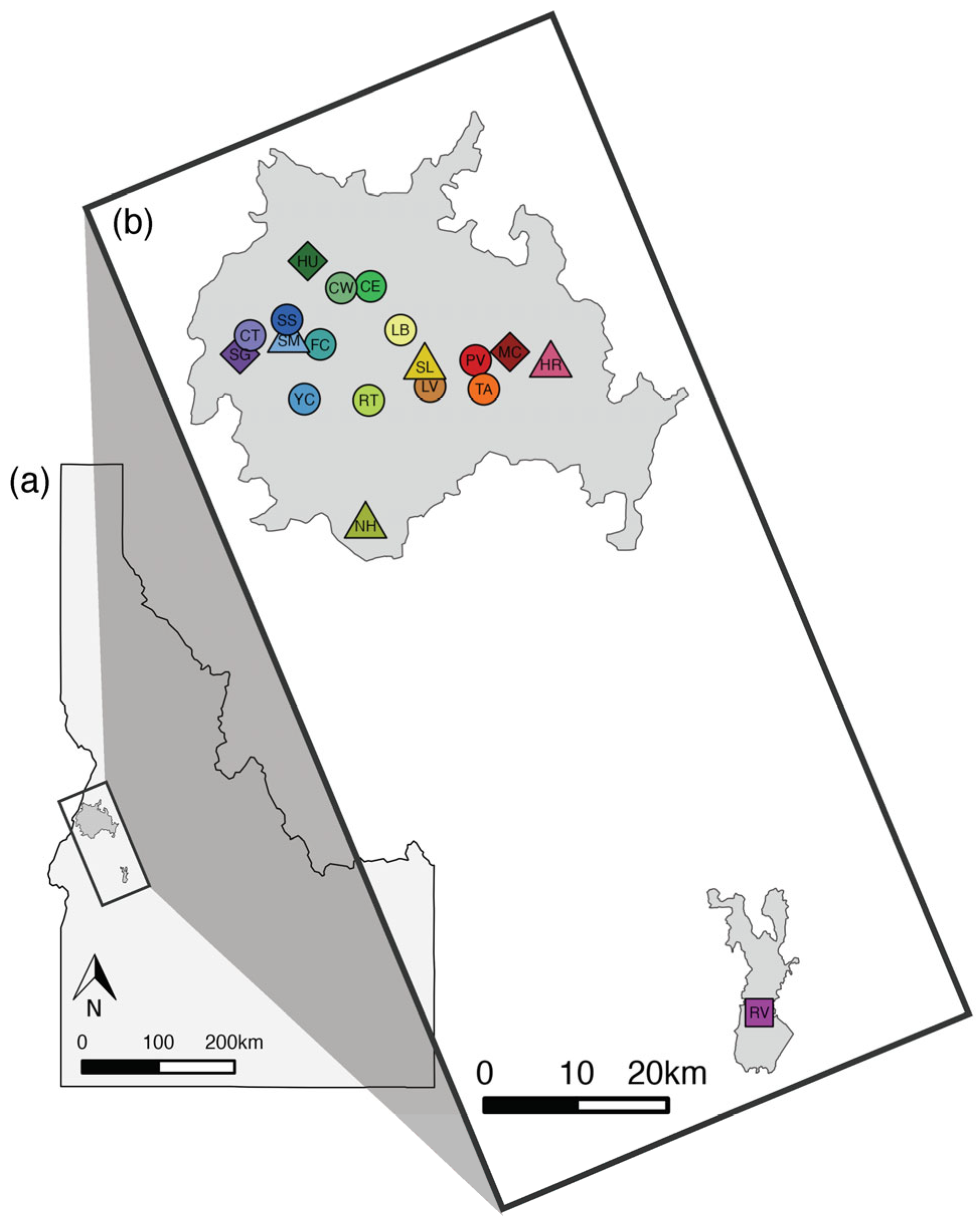
2.1. Study Area and Sample Collection

To capture individuals, Tomahawk live traps (Tomahawk Live Trap Co., Hazelhurst, WI, USA; 13 × 13 × 41 cm and 15 × 15 × 50 cm) were baited and placed near burrows or logs at regularly spaced intervals within occupied sites in 2016 and 2020 [42,43,47] (Figure 1, Table 1). All study sites were located in Adams and Valley Counties, Idaho, spread throughout the extant range of the NIDGS. Study site elevations ranged from 1060 m to 1700 m. The mean annual precipitation for the past 10 years at the study sites was 715 mm, most of which fell as winter snow. Study sites were within a landscape that included coniferous forest interspersed with riparian corridors, rocky scabs, and meadows. Ponderosa pine (Pinus ponderosa) and Douglas fir (Pseudotsuga menziesii) dominated the overstory in forested areas at our study sites. Common forest understory plants included snowberry (Symphoricarpos spp.), spiraea (Spiraea spp.), pine grass (Calamagrostis rubescens), elk sedge (Carex geyeri), heart-leaf arnica (Arnica cordifolia), and wild strawberry (Fragaria spp.). Common plants in xeric meadows included big sagebrush (Artemisia tridentata), bluegrass (Poa spp.), bromes (Bromus spp.), buckwheat (Eriogonum spp.), wild onion (Allium spp.), and biscuitroot (Lomatium spp.). Cattle grazing, hunting, and camping were common human land uses, though human presence on our study sites was rare.
We swabbed the inside of each captured squirrel’s cheek with a sterile cotton swab (Lakewood Biomedical, Dallas, TX, USA) to collect epithelial cells, which we repeated five times per individual. All replicate buccal swabs per individual were preserved in the same tube in ATL buffer (QIAGEN, Inc., Venlo, Netherlands) until DNA extraction. All NIDGS were trapped and handled following protocols and procedures approved by the University of Idaho Animal Care and Use Committee (IACUC #2015-53 and #2019-28). Our activities were approved under an Idaho Department of Fish and Game scientific collecting permit (SCP #120629) and a U.S. Fish and Wildlife Service recovery permit (TE94776A-3).

2.2. GT-seq Library Preparation, Sequencing, and Genotyping

We used Qiagen Blood and Tissue extraction kits (QIAGEN, Inc.) to extract DNA from buccal swab samples using standard protocols. The buccal swab samples were extracted in a low-quantity DNA facility with no PCR products or high quantity DNA sources.
Detailed steps of the GT-seq panel SNP selection, primer development, optimization, library preparation, and genotyping are described in Garrett et al. [48]. We sequenced seven GT-seq libraries of buccal swab extracts using a single-read 118 bp cycle on Illumina NovaSeq SP at the University of Oregon Genomics and Cell Characterization Core Facility (G3CF) and a paired-end 75 bp cycle on Illumina NextSeq at Seqmatic LLC (San Francisco, CA, USA). We used the GT-seq pipeline v. 3 on GitHub (https://github.com/GTseq, accessed on 4 June 2024) for demultiplexing and genotyping, which was chosen after comparison among genotyping methods and validation against RAD sequencing data [47]. After testing different allele ratios for calling heterozygotes, we modified the GTseq_Genoytper_v3.pl script to call heterozygotes with an allele ratio between 0.4 and 2.5, from the original 0.2–2.0 range. Using the R package ADEGENET v2.1.10 [49], individuals were removed with missing values greater than 25% and loci were removed with missing values greater than 50%. Monomorphic loci were also removed. Additionally, loci with a per locus FIS value less than −0.15 were also removed.
For each site per year, we used the basic.stats function from HIERFSTAT R package v0.5-11 [50] to estimate observed and expected heterozygosity. From the private_alleles function from POPPR R package v2.9.4 [51], we quantified private alleles per site per year.
We estimated the isolation by distance (IBD) using the mantel function in the VEGAN R package v2.6-4 [52] for both 2016 and 2020 separately. We estimated IBD with two metrics of genetic distance with all loci, as well as neutral and putatively adaptive loci independently, for 2016 and 2020. We used the as.dist function in HIERFSTAT R package v0.5-11 [50] to calculate pairwise FST and the dist.genpop function in ADEGENET R v2.1.10 package [49] to calculate Nei’s genetic distance. We compared genetic distances for each site with ≥6 samples against pairwise Euclidean distances for all sites. We calculated IBD correlation coefficients using both Pearson (with and without the log transformation of Euclidean distance) and Spearman’s rank correlation. Below, we describe IBD results for FST and Spearman’s rank correlation, but all are included in the Supplementary Materials.

2.3. Evolutionarily Significant Units

We estimated reproductive isolation and evolutionary potential through exploring population structure and genetic differentiation by using neutral and putatively adaptive SNPs. First, we performed principal component analysis (PCA) to visually inspect population structure. We used the dudi.pca function in ADE4 R package v5.7-1 [53] then the ggplot function in GGPLOT2 v3.5.0 package to create the PCA plots [54]. Next, we used the Bayesian clustering analysis as implemented in program STRUCTURE v2.3.4 [55]. We applied an admixture model with a burn-in period of 100,000 and a run length of 500,000 MCMC replicates to determine the number of genetic clusters (K) from 1 to 20 over 10 iterations each. We identified the optimal K for each dataset according to the Evanno method [56] and the rate of change in the likelihood values [55]. We visualized STRUCTURE outputs with bar-plots and geographic pie charts using the following R script (https://github.com/sakura81/PYRA_Genomics, accessed on 4 June 2024) and R package SCATTERPIE v0.2.1 [57]. We also quantified private alleles per ESU once they were defined.

2.4. Management Units
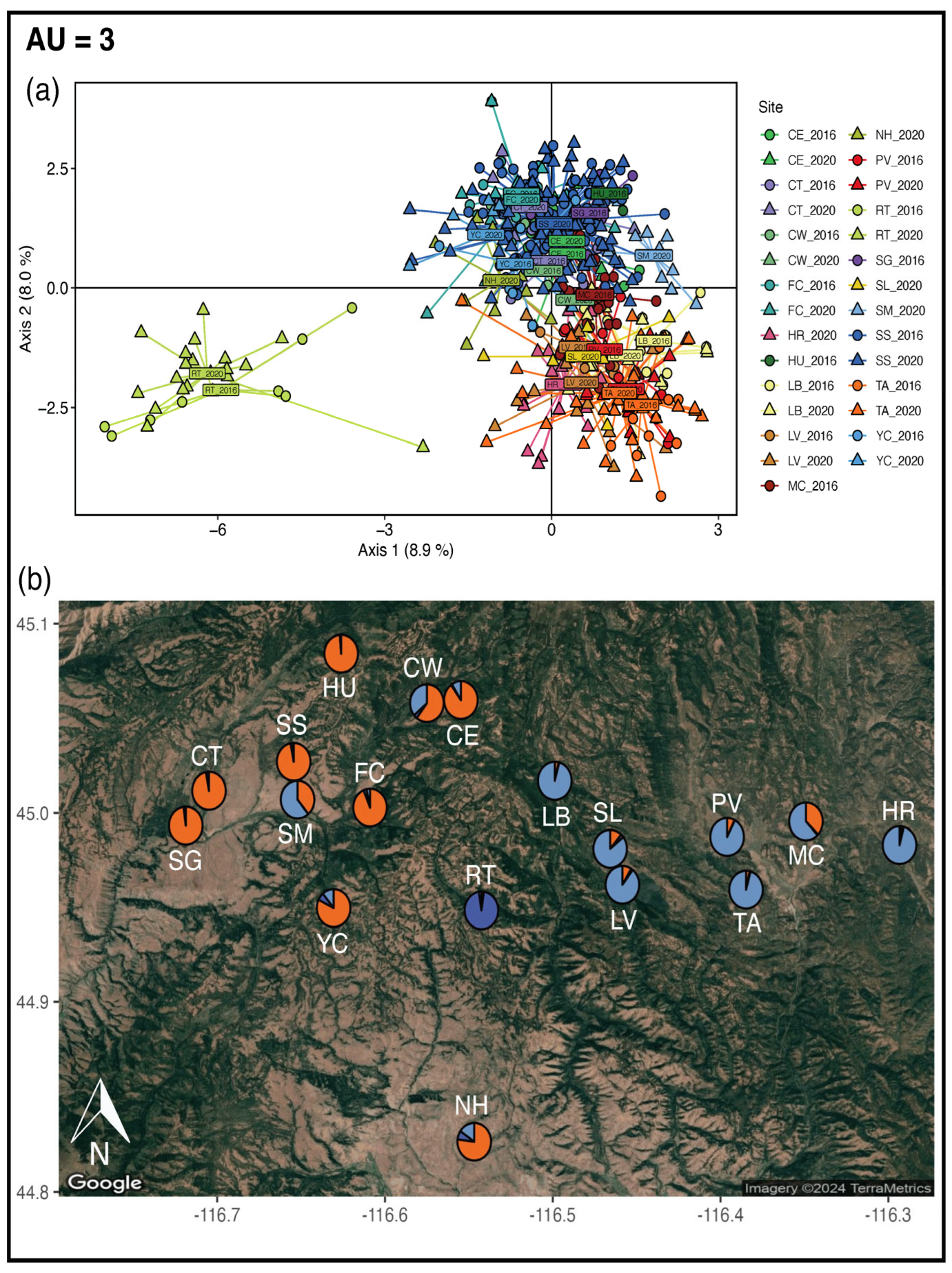
We investigated current population structure with the same PCA and STRUCTURE techniques described above using only neutral SNPs. We calculated pairwise FST with only neutral loci with function boot.ppfst in HIERFSTAT R package v0.5-11 [50] with 999 bootstraps to estimate genetic distinctiveness.
We used the program Population Graphs as implemented in the POPGRAPHS R package v1.5.3 [58] to assess gene flow and connectivity among sites. The program uses a graph theory approach to describe genetic covariance among sites (i.e., nodes), where connections (i.e., edges) between sites represent genetic exchange. Edges between nodes may represent dispersal corridors or connecting habitat patches, or more aspatial theoretical connections, but are an important indicator that gene flow between nodes is possible if gene flow is not actively occurring [59,60,61]. We visualized gene flow using a cutoff of 0.90 [23]. We calculated two measures of connectivity between nodes: betweenness, the number of times that a node acts as a bridge along the shortest path between two other nodes, and degree, the total number of edges connected to a particular node in a graph [60,62,63].
After we delineated MUs, we estimated Ne for each MU using the linkage disequilibrium method of NeEstimator v2.01 [64] for 2016 and 2020 separately. We estimated Ne with the linkage disequilibrium method as we did not sample the same individuals over multiple time periods. We only included neutral SNPs and excluded alleles with frequencies less than a critical value of 0.05. Additionally, observed heterozygosity was calculated for each MU.

2.5. Adaptive Units

We quantified adaptive differentiation with PCA and STRUCTURE as described above but using only adaptive SNPs. For 2016 and 2020 separately, we tested for private alleles in candidate AU arrangements of K = 3, 4, and 5 to examine how adaptive allelic variation is spread across the species range at different grouping levels.

2.6. The Spatially Disjunct Population of Round Valley

While most NIDGS subpopulations occur in a 29 km × 37 km area in Adams County, the southernmost population, Round Valley (RV), is ~70 km from all other populations and is restricted to a 3 km × 4 km area in Valley County (Figure 1). We obtained one tissue sample from Round Valley in 2022 and sequenced it with the NIDGS GT-seq panel. We included this one sample in PCA with all the other buccal swab samples and quantified private alleles for Round Valley as compared to all other sites. We acknowledge that we cannot draw any statistical conclusions with just one sample, but the sample can provide preliminary information on how divergent Round Valley may be compared to the other populations.

3. Results

3.1. Genotyping

Sequencing yielded 201,904 mean reads per individual (range = 10–18,802,287) and 116,184 mean on-target reads per individual (range = 1–11,219,616). After filtering, the final dataset included 182 neutral and 70 putatively adaptive SNPs (total = 252 SNPs). Two samples were removed due to possible laboratory contamination or mislabeling/mishandling of samples. For 2016, there were 201 individuals from 14 sites with a mean sample size per site of 14. For 2020, there were 207 individuals from 18 sites with a mean sample size per site of 18 (Table 1).
For all sites except for Rocky Top (RT), observed heterozygosity was highest with neutral SNPs only, followed by all SNPs, then putatively adaptive SNPs (Table 1). For Rocky Top only, observed heterozygosity was greatest with putatively adaptive SNPs. When private alleles were quantified for all sites, Rocky Top had 12 loci and YCC had 1 locus with private alleles in 2016 (Table 1). In 2020, only Rocky Top had seven loci with private alleles. Across all years, all private alleles were associated with putatively adaptive SNPs.
We identified a significant pattern of IBD for both years when calculated with all SNPs and neutral SNPs (2016 all SNPs, r = 0.224, p-value = 0.034; 2016 neutral SNPs, r = 0.339, p-value = 0.007; 2020 all SNPs, r = 0.361, p-value = 0.012; 2020 neutral SNPs, r = 0.371, p-value = 0.007). When calculated with adaptive SNPs, IBD was significant for 2020 (r = 0.361, p-value = 0.013) but not for 2016 (r = 0.0458, p-value = 0.34; Table S1).

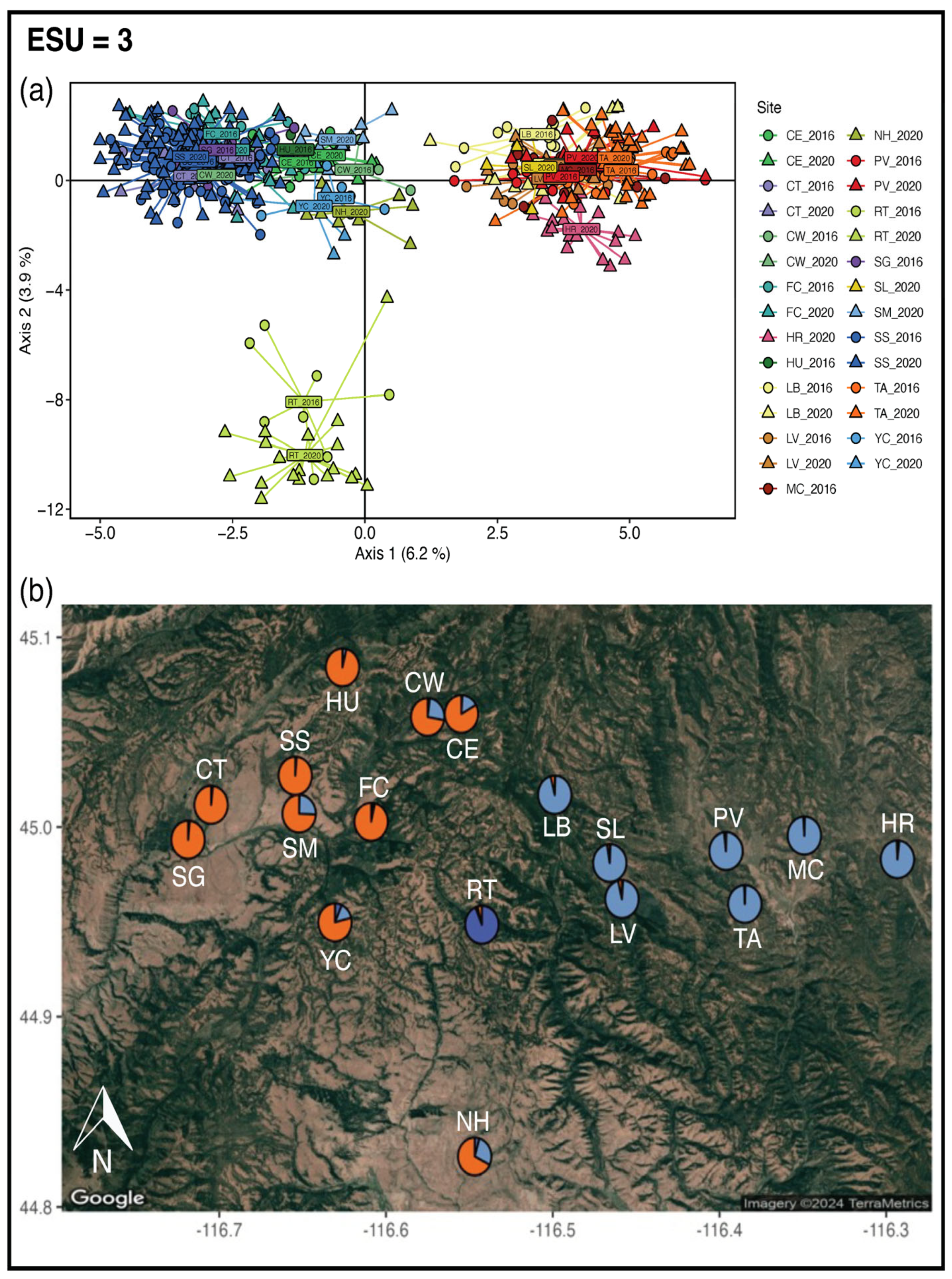
3.2. Evolutionarily Significant Units

The PCA performed with all SNPs identified three main groups: a western group, an eastern group, and only Rocky Top (Figure 2 and Figure S1). These groupings are also identified in STRUCTURE at K = 3, though the best supported K for STRUCTURE is K = 2 based on the Evanno method and K = 8 with the likelihood method (Figures S2 and S3). Due to Rocky Top’s distinctiveness in the PCA, its large number of private alleles, and that it is the first site to differentiate at K = 3, we have identified three ESUs: (1) a West ESU, (2) an East ESU, and (3) an ESU with only Rocky Top. The West ESU includes Summit Gulch (SG), Cap Gun/Tree Farm (CT), Steve’s Creek/Squirrel Valley/Manor (SS), Smith Mountain (SM), YCC (YC), Huckleberry (HU), Fawn Creek (FC), Cold Springs West (CW), Cold Springs East (CE), and North Hornet (NH). The East ESU consists of Lower Butter (LB), Slaughter Gulch (SL), Lost Valley (LV), Price Valley (PV), Tamarack (TA), Mud Creek (MC), and Hot Springs Road (HR). Each ESU has its own private alleles across 6 neutral and 5 putatively adaptive SNPs: 4 alleles for the West ESU, 5 alleles for the East ESU, and 2 alleles for the Rocky Top ESU (Table S2).

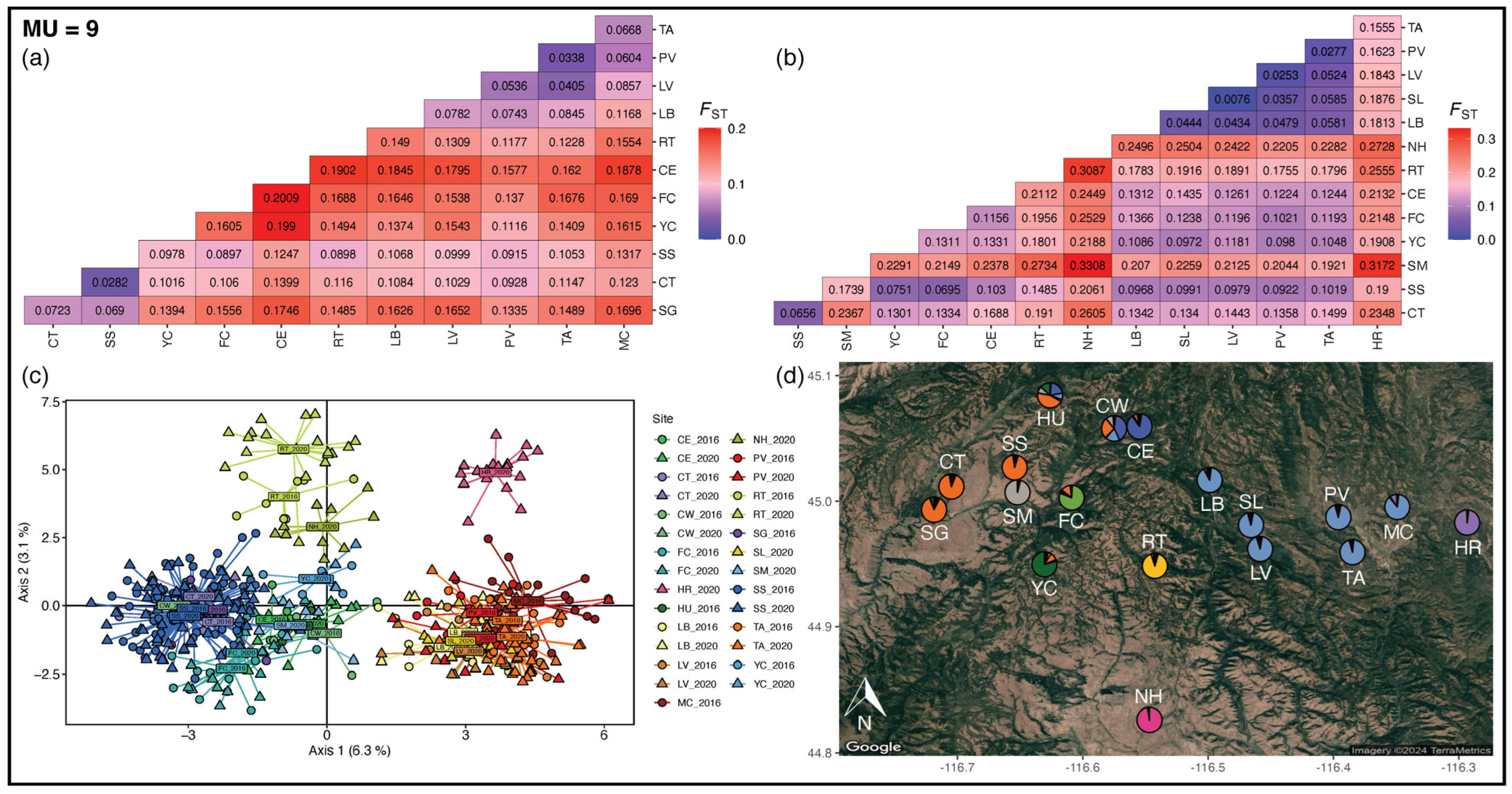
3.3. Management Units

To delineate management units across population groups, we combined multiple analyses of demographic connectivity. We found significant levels of differentiation from pairwise FST estimates by site (Figure 3, Table S3). All pairwise FST estimates were significantly different from zero in 2016, and all but two estimates in 2020 showed significant pairwise FST. The majority of pairs of sites had FST greater than 0.1 in 2016 and 2020, 71% and 78%, respectively (Figure S7). We detected strong genetic differentiation among populations; 32% (in 2016) and 52% (in 2020) of FST estimates were greater than Wright’s [65] 0.15 threshold for strong genetic differentiation. For 2016, the mean and median FST across all sites was 0.137 and 0.131 (range: 0.028–0.201), respectively. For 2020, the mean and median FST across all sites was 0.159 and 0.156 (range: 0.007–0.331), respectively.
In the network analyses, we found that all sites were connected to at least one other site, and each year, all sites were connected to one another (Figure 4, Table 1). For 2016, we found a mean degree of 6 edges (range: 4–10) and a mean betweenness of 14 (range: 0–30) (Table 1). For 2020, we found a mean degree of 5 edges (range: 2–10) and a mean betweenness of 16.6 (range: 0–40).
The PCA revealed very similar genetic structure as ESUs: a western and an eastern grouping (Figure 3), where western sites were more spread across PC1 and sites on the periphery of the ranges are also distinct (Hot Springs Road and North Hornet). Hot Springs Road, North Hornet, Fawn Creek, Cold Springs East, and Smith Mountain differentiate along PC3 and PC4 (Figure S1).
The best supported value of K from STRUCTURE was K = 2 using the Evanno method and K = 9 using the likelihood method (Figure S2). The fine-scale structure supported by PCA and pairwise FST align with K = 9 in STRUCTURE (Figure 3 and Figure S4). Therefore, we have delineated 9 MUs: (1) West MU of Summit Gulch, Cap Gun/Tree Farm, Steve’s Creek/Squirrel Valley/Manor, and Huckleberry, (2) Smith Mountain, (3) YCC, (4) Fawn Creek, (5) Cold Springs MU of Cold Springs West and Cold Springs East, (6) Rocky Top, (7) North Hornet, (8) East MU of Lower Butter, Slaughter Gulch, Lost Valley, Price Valley, Tamarack, and Mud Creek, and (9) Hot Springs Road.
With NeEstimator, we found that Ne was variable among MUs (mean 38.16, range: 2.3–220.9) and was influenced by how many sites were within an MU (Table 2). The majority of MUs had an Ne less than 50 individuals in 2016 and 2020, 67% (4/6 MUs) and 78% (7/9 MUs), respectively.

3.4. Adaptive Units

With adaptive SNPs, the PCA results agree with the STRUCTURE analyses (Figure 5). With STRUCTURE, K = 3 (with a subpeak at K = 5) is best supported using the Evanno method and K = 5 is supported with the likelihood method (Figures S2 and S5). There were no differences in the number of private alleles among Ks 3, 4, or 5 (Table S4). Moreover, all private alleles were represented at K = 3 that were also present at Ks 4 and 5. Therefore, we have designated three AUs: (1) West AU, (2) East AU, and (3) an AU with just Rocky Top. The only difference between the AUs and the ESUs is that Smith Mountain is in the East AU, while it is in the West ESU.

3.5. The Distant Population of Round Valley

With only a single sample, we did not have enough data to fully include the isolated Round Valley population in our conservation unit analysis. The sample from Round Valley falls more closely with the west than the east group in PCAs with all, neutral, and adaptive SNPs (Figure S6). In the PCAs with all and neutral SNPs, Round Valley aligns with North Hornet, which is the geographically closest site to Round Valley. Round Valley is the most distinct along PC3 with only adaptive SNPs. Round Valley has no private alleles compared to the other sites.

4. Discussion

Through the application of a GT-seq panel in NIDGS [48], we were able to assess neutral and adaptive genetic variation to delineate conservation units, assess recovery goals, and help guide future management actions. Specifically, we delineated 3 ESUs, 9 MUs, and 3 AUs. The West ESU has 7 MUs, the East ESU has 2 MUs, and the Rocky Top ESU has 1 MU. The ESUs and AUs align with each other except for the assignment of one site. Across sites and conservation units, we quantified genetic variation, genetic structure, connectivity, and Ne to address species recovery objectives to gauge the effects of previous management actions and guide future decision making.

4.1. Evolutionarily Significant Units

We found support for reproductive isolation in terms of the Waples [25] definition of ESUs. We detected clear separation among the west and east group in STRUCTURE results, with little to no admixture within individuals or sites (Figure 2 and Figure S3). This is also mirrored in the PCA results, where no individuals from either the west or the east fall out in the opposite grouping (Figure 2 and Figure S1). The division of a west and east group is supported by past NIDGS genetics work with mitochondrial DNA, nuclear microsatellites, and SNPs through PCA, STRUCTURE, and population graph analyses [42,43,47,66]. Broad scale population structure is likely most influenced by topographical features that serve as dispersal barriers, as west and east sites are separated by a mountain range [66]. Movement of NIDGS is less likely to occur over mountain ridges and would follow contour lines or rivers when possible [67].
Our ESU results support the Waples [25] definition of ESUs representing evolutionary distinctiveness. Private alleles (i.e., unique genetic variants) are found within each ESU (Table S3). These alleles occur at both neutral and adaptive SNPs, which highlights that both genetic drift and selection may be contributing to divergence among the ESUs. Further, Rocky Top has the majority of private alleles when estimated per site, which are all associated with adaptive SNPs (Table 1). Gene flow may be limited to/from Rocky Top, and the unique habitat features of the site may have been selected for genetic variants unique to Rocky Top. For example, the soil is shallower and rockier with more sagebrush (Artemisia spp.) and less grass than other sites. Rocky Top is one of the higher elevation sites in our study (~1700 m). Phenological differences have been documented to vary by elevation across the NIDGS range, with squirrels at higher elevations immerging into and emerging from hibernation later with consequently shorter active seasons than squirrels at lower elevations [35]. Additionally, while we did not find any private alleles for the distant population Round Valley, we believe that further sampling of Round Valley is needed to assess its potential status as an ESU.

4.2. Management Units

Connectivity among occupied sites has been explored by previous NIDGS genetic studies, which have revealed patterns of fine-scale differentiation. Based on population graph analysis using microsatellite loci, the western sites had higher levels of connectivity with each other than sites in the east [66]. Connectivity within the western group was also found to be higher in previous STRUCTURE analyses, with sites sharing the same ancestral group at higher levels of K than the east sites [42,67]. However, assignment tests with microsatellites revealed a low level of exchange (9.38–23.08% mis-assignment) between sites overall, with sites in the east having slightly higher levels of mis-assignment than to sites in the west [43,67]. Fine-scale population structure is also supported by low to moderate levels of pairwise FST reported across multiple studies [36,43,47]. The higher levels of differentiation in the east may be a consequence of loss of suitable habitat and dispersal corridors which has led to population isolation [36,38].
The levels of connectivity that affect genetic processes of drift and selection are different from the levels of connectivity that affect demographics. Genomic data alone cannot quantify demographic independence given that low rates of migration can maintain genetic similarity without causing significant demographic interdependence among populations [68]. For example, in our study we identified substantially more MUs than ESUs, reflecting lower levels of migration which create shared evolutionary history but not demographic connection. Given the fragmented habitat and limited dispersal of NIDGS [66], our identification of nine MUs within a relatively small area for this species is consistent with our previous understanding of these populations. In a previous gravity model intended to analyze functional connectivity for the NIDGS, site productivity and topography had the most effect on gene flow, suggesting these variables likely contribute to the fine-scale population structure we identified [66]. However, variables describing land cover, interspecific competition, and human disturbance were not found to impact functional connectivity [66]. To further our understanding of connectivity and demographic independence across the entire NIDGS range, further sampling at Round Valley is needed to assess its own classification as an MU given its geographic isolation.
The role of IBD in delineating MUs is also important to consider, as patterns of genetic differences are often correlated with geographic distance. Isolation by distance is fairly prominent across taxa and is not surprising for a small terrestrial mammal [69], but its significance here emphasizes that straight distance hinders connectivity among populations. An IBD relationship in NIDGS has been reported in some [42,47,66] but not all [43] prior studies. Each prior study examined a different subset of sites, and the inclusion or exclusion of different sites are important to consider in estimating the effect of geographic distance on allele frequencies. With the inclusion of samples from the peripheral sites, North Hornet and Hot Springs Road, the current study has a relatively larger geographic extent than previous studies.

4.3. Adaptive Units

Putatively adaptive SNPs for the GT-seq panel were originally identified with RADseq [42], with most of the sites in our study included in the RADseq SNP genotyping. That study used minimally invasive sampling and produced a final dataset of fewer than 4000 SNP loci, so there may be adaptive variation not included in the GT-seq panel. In Barbosa et al. [42], elevation appeared to be the main driver of adaptive differentiation between sites, and putatively adaptive SNPs were associated with environmental variables such as slopes, ridges, and peaks, as well as soil particle size. Further, the three populations that were the most distinct in the partial redundancy analysis (pRDA), Rocky Top, Lower Butter, and Tamarack, also showed separation in our PC axes 3 and 4 (Figure S1).
We identified five putatively adaptive SNPs that have private alleles among the three AUs. Gene ontology enrichment analyses, however, found no evidence for enrichment of specific molecular functions or biological processes linked with the putatively adaptive SNPs [42]. The only difference between the three ESUs and the three AUs is that Smith Mountain is grouped in the West ESU but within the East AU. In both analyses, this site showed evidence of shared ancestry with both the East and West groups. We only had 10 samples from Smith Mountain, and it would be valuable to continue sampling NIDGS at this site to understand local adaptation and connectivity of this population.

4.4. Management and Conservation Implications

We have more clearly defined the NIDGS metapopulation structure by evaluating genetic differentiation and connectivity. To be defined as a metapopulation, habitat patches/sites must represent independent breeding populations that are nonetheless connected to some extent to allow for recolonization following local extinction [70]. We found strong evidence that NIDGS form a loosely connected meta-population with strong genetic differentiation. However, despite the large degree of genetic differentiation between our sub-populations, they nonetheless represent a metapopulation rather than fully distinct populations. In a functioning metapopulation, patches/sites are connected to at least one other patch/site via gene flow [60]. In our population graph analysis, we found that all sites were connected. We did not include Round Valley in the Population Graph analysis, but it is likely isolated. Round Valley is ~15 km south of Lake Cascade and sits between two mountain ridges, which, as previous analyses suggest [66], are barriers to dispersal.
According to the species recovery plan, the NIDGS may be considered for delisting when ten subpopulations maintain an average Ne of greater than 500 individuals for five consecutive years. From our estimates, no MU, and therefore no single subpopulation, has reached this recovery threshold. Seven out of nine MUs have an Ne under 50 individuals, which is proposed to be the minimum Ne necessary for preventing short-term inbreeding effects (but see [71,72]). However, the high Ne in the West MU relative to the other MUs may suggest that it could be an important source population or buffer against population fluctuations in other parts of the species’ range. The West MU currently has the most samples available for analyses, and increased sampling within the other MUs would provide more accurate Ne estimates for all MUs. Given the current fragmented habitat for this species, the recovery goal of Ne > 500 across ten subpopulations may be difficult to achieve.
Population genetic metrics and conservation unit delineation assessed from genomic data can guide management decisions to preserve both short- and long-term species viability and persistence. In the short-term, priority is best placed on MUs with low levels of genetic diversity or Ne, or those where Ne is declining, because management units with low genetic diversity and Ne are at higher risk of reduced fitness and loss of evolutionary potential [73]. Conserving small MUs is also critical to prevent against local extinction due to ecological or stochastic processes, such as predation [74], interspecific competition [75], and disease [44,45]. For NIDGS, conservation efforts may be most effective to focus on the three MUs (West, YCC, and Rocky Top) for which we detected a decrease in diversity and Ne between 2016 and 2020, and two MUs (Smith Mountain and North Hornet) that had the lowest observed heterozygosity.
Maintaining connectivity within ESUs is more critical than maintaining connectivity between ESUs. To maintain connectivity within ESUs, it is most important to maintain dispersal corridors that link populations with small Ne to reduce risks associated with genetic drift and inbreeding. Previous modeling suggests that prescribed burns would improve NIDGS habitat by reducing conifer density, increasing herbaceous community cover, and creating an open understory [39], but a recent experimental study that tested these predictions did not find evidence that using prescribed burning is effective [76].
In the long-term, it is important to maintain adaptive variation among ESUs/AUs, because it determines long-term species viability, as well as the potential for species distribution or population size to increase [15]. It is vital to conserve species-wide adaptive diversity, especially in species composed of small, isolated subpopulations, to maintain evolutionary potential and counteract the influence of genetic drift [73]. Therefore, Rocky Top is valuable as an isolated ESU/AU and more explicit studies on the Rocky Top population may help identify its unique attributes. Rocky Top shows signs of high adaptive genetic variation, which may harbor capacity to respond or adapt to environmental change. For example, NIDGS hibernation behavior is sensitive to changes in snowfall, ambient temperature, and food availability, and altered hibernation emergence will likely impact survival [35]. Habitat features that reduce the risk of predation, during both the active season and the hibernation season, are important to identify as well as the habitat features that buffer NIDGS from harsh weather conditions. For instance, snowpack during hibernation may be important for both reducing predation and ameliorating suboptimal temperatures [35]. Future climate projections for west-central Idaho predict more rain and less snow [77]; therefore, NIDGS may experience a suite of selection pressures that have not been present in their evolutionary history. As such, maintaining genetic variation will be especially critical for the species’ persistence as the climate changes. Additionally, for management actions like translocations or genetic rescue, only moving individuals from within ESUs/AUs would minimize the risk of outbreeding depression [78,79].
The continuation of genetic monitoring into the future is critical to evaluate the effects of management action or stochastic events. The GT-seq panel developed for the NIDGS [48] is a useful tool for monitoring allele frequencies and gene diversity at both neutral and putatively adaptive SNPs as more samples are collected over time. Estimates of gene flow between sites or detections of migration can identify potential dispersal corridors that can be maintained by habitat protection or restoration. Checking for losses of heterozygosity or decreases of Ne will provide insights on the effects of inbreeding. Genetic monitoring in NIDGS that includes estimates of genetic drift and inbreeding, as well as adaptive variation, will best inform estimates of species persistence. The inclusion of future samples from previously sampled sites or new sites will validate or adjust conservation unit delineation and will help with the prioritization of resource allocation to conservation units. The inclusion of other data types, like ecological or behavioral data, would be valuable to collect and incorporate to confirm or re-evaluate conservation units. Overall, genomic data provides critical information that can directly assess recovery goals and actions for this threatened species.

Supplementary Materials

The following supporting information can be downloaded at: https://www.mdpi.com/article/10.3390/genes16060694/s1, Figure S1: PC axes 3 and 4 for all, neutral, and adaptive SNPs; Figure S2: Evanno and likelihood plots for identifying the best K for STRUCTURE for all, neutral, and adaptive SNPs; Figure S3: STRUCTURE bar plots with all SNPs; Figure S4: STRUCTURE bar plots with neutral SNPs; Figure S5: STRUCTURE bar plots with adaptive SNPs; Figure S6: PCA outputs with site Round Valley; Figure S7: Pairwise FST with all SNPs and adaptive SNPs; Table S1: Mantel test metrics; Table S2: Private alleles per ESU per year; Table S3: Pairwise FST confidence intervals with neutral SNPs; Table S4: Private alleles per MU per year.

Author Contributions

Conceptualization, M.J.G., C.J.C., L.P.W. and P.A.H.; investigation, M.J.G.; writing—original draft preparation, M.J.G.; writing—review and editing, C.J.C., L.P.W. and P.A.H.; funding acquisition, C.J.C., L.P.W. and P.A.H. All authors have read and agreed to the published version of the manuscript.

Funding

This research was funded by the NSF Idaho EPSCoR Program and by the National Science Foundation under award number OIA-1757324. The U.S. Forest Service (Payette National Forest), U.S. Fish and Wildlife Service, and Idaho Department of Fish and Game provided funding that allowed for the capture and sampling of northern Idaho ground squirrels.

Institutional Review Board Statement

This study was performed under the auspices of University of Idaho IACUC protocols #2015-53, 2019-28 and 2022-10.

Data Availability Statement

Genotyping pipelines, custom scripts, and the GT-seq SNP dataset in .csv format are available on GitHub (https://github.com/mjgarrett/NIDGS_scripts, accessed on 4 June 2024). VCF files from the RADseq data are available on Dryad (https://doi.org/10.5061/dryad.sj3tx965c, accessed on 4 June 2024).

Acknowledgments

We thank Austin Allison, Alice Morris, and many seasonal field technicians for their help obtaining samples, Jennifer Adams for assistance with laboratory work, and the OX Ranch for providing field lodging for the field crew collecting samples. Any use of trade, firm, or product names is for descriptive purposes only and does not imply endorsement by the U.S. Government.

Conflicts of Interest

The authors declare no conflicts of interest.

References

  1. Allendorf, F.W. Genetics and the conservation of natural populations: Allozymes to genomes. Mol. Ecol. 2017, 26, 420–430. [Google Scholar] [CrossRef]
  2. Allendorf, F.W.; Funk, W.C.; Aitken, S.N.; Byrne, M.; Luikart, G. Conservation and the Genomics of Populations; Oxford University Press: Oxford, UK, 2022; ISBN 978-0-19-259857-8. [Google Scholar]
  3. Allendorf, F.W.; Luikart, G.H.; Aitken, S.N. Conservation and the Genetics of Populations; Wiley-Blackwell: Malden, MA, USA, 2012. [Google Scholar]
  4. Frankham, R. Inbreeding in the wild really does matter. Heredity 2010, 104, 124. [Google Scholar] [CrossRef] [PubMed]
  5. Nonaka, E.; Sirén, J.; Somervuo, P.; Ruokolainen, L.; Ovaskainen, O.; Hanski, I. Scaling up the effects of inbreeding depression from individuals to metapopulations. J. Anim. Ecol. 2019, 88, 1202–1214. [Google Scholar] [CrossRef] [PubMed]
  6. Palstra, F.P.; Ruzzante, D.E. Genetic estimates of contemporary effective population size: What can they tell us about the importance of genetic stochasticity for wild population persistence? Mol. Ecol. 2008, 17, 3428–3447. [Google Scholar] [CrossRef]
  7. Waples, R.S. What is Ne, anyway? J. Hered. 2022, 113, 371–379. [Google Scholar] [CrossRef] [PubMed]
  8. Hedrick, P.W.; Gilpin, M.E. Genetic effective size of a metapopulation. In Metapopulation Biology; Hanski, I., Gilpin, M.E., Eds.; Academic Press: San Diego, CA, USA, 1997; pp. 165–181. ISBN 978-0-12-323445-2. [Google Scholar]
  9. Kurland, S.; Ryman, N.; Hössjer, O.; Laikre, L. Effects of subpopulation extinction on effective size (Ne) of metapopulations. Conserv. Genet. 2023, 24, 417–433. [Google Scholar] [CrossRef]
  10. Ryman, N.; Laikre, L.; Hössjer, O. Variance effective population size is affected by census size in sub-structured populations. Mol. Ecol. Resour. 2023, 23, 1334–1347. [Google Scholar] [CrossRef]
  11. Frankham, R. Genetics and extinction. Biol. Conserv. 2005, 126, 131–140. [Google Scholar] [CrossRef]
  12. Lande, R. Risks of population extinction from demographic and environmental stochasticity and random catastrophes. Am. Nat. 1993, 142, 911–927. [Google Scholar] [CrossRef]
  13. Baalsrud, H.T.; Sæther, B.E.; Hagen, I.J.; Myhre, A.M.; Ringsby, T.H.; Pärn, H.; Jensen, H. Effects of population characteristics and structure on estimates of effective population size in a house sparrow metapopulation. Mol. Ecol. 2014, 23, 2653–2668. [Google Scholar] [CrossRef]
  14. Hastings, A.; Harrison, S. Metapopulation dynamics and genetics. Annu. Rev. Ecol. Syst. 1994, 25, 167–188. [Google Scholar] [CrossRef]
  15. Hohenlohe, P.A.; Funk, W.C.; Rajora, O.P. Population genomics for wildlife conservation and management. Mol. Ecol. 2021, 30, 62–82. [Google Scholar] [CrossRef]
  16. Walters, A.D.; Schwartz, M.K. Population genomics for the management of wild vertebrate populations. In Population Genomics: Wildlife; Hohenlohe, P.A., Rajora, O.P., Eds.; Springer: Cham, Switzerland, 2020; pp. 419–436. [Google Scholar]
  17. Campbell, N.R.; Harmon, S.A.; Narum, S.R. Genotyping-in-thousands by sequencing (GT-Seq): A cost effective SNP genotyping method based on custom amplicon sequencing. Mol. Ecol. Resour. 2015, 15, 855–867. [Google Scholar] [CrossRef]
  18. Burgess, B.T.; Irvine, R.L.; Russello, M.A. A Genotyping-in-thousands by sequencing panel to inform invasive deer management using noninvasive fecal and hair samples. Ecol. Evol. 2022, 12, e8993. [Google Scholar] [CrossRef]
  19. Hayward, K.M.; Clemente-Carvalho, R.B.G.; Jensen, E.L.; de Groot, P.V.C.; Branigan, M.; Dyck, M.; Tschritter, C.; Sun, Z.; Lougheed, S.C. Genotyping-in-thousands by sequencing (GT-Seq) of noninvasive faecal and degraded samples: A new panel to enable ongoing monitoring of Canadian polar bear populations. Mol. Ecol. Resour. 2022, 22, 1906–1918. [Google Scholar] [CrossRef]
  20. Schmidt, D.A.; Campbell, N.R.; Govindarajulu, P.; Larsen, K.W.; Russello, M.A. Genotyping-in-thousands by sequencing (GT-Seq) panel development and application to minimally invasive DNA samples to support studies in molecular ecology. Mol. Ecol. Resour. 2020, 20, 114–124. [Google Scholar] [CrossRef] [PubMed]
  21. Barbosa, S.; Mestre, F.; White, T.A.; Paupério, J.; Alves, P.C.; Searle, J.B. Integrative approaches to guide conservation decisions: Using genomics to define conservation units and functional corridors. Mol. Ecol. 2018, 27, 3452–3465. [Google Scholar] [CrossRef] [PubMed]
  22. Boussarie, G.; Momigliano, P.; Robbins, W.D.; Bonnin, L.; Cornu, J.-F.; Fauvelot, C.; Kiszka, J.J.; Manel, S.; Mouillot, D.; Vigliola, L. Identifying barriers to gene flow and hierarchical conservation units from seascape genomics: A modelling framework applied to a marine predator. Ecography 2022, 2022, e06158. [Google Scholar] [CrossRef]
  23. Forester, B.R.; Murphy, M.; Mellison, C.; Petersen, J.; Pilliod, D.S.; Van Horne, R.; Harvey, J.; Funk, W.C. Genomics-informed delineation of conservation units in a desert amphibian. Mol. Ecol. 2022, 31, 5249–5269. [Google Scholar] [CrossRef]
  24. Weckworth, B.V.; Hebblewhite, M.; Mariani, S.; Musiani, M. Lines on a map: Conservation units, meta-population dynamics, and recovery of woodland caribou in Canada. Ecosphere 2018, 9, e02323. [Google Scholar] [CrossRef]
  25. Waples, R.S. Pacific Salmon, Oncorhynchus Spp., and the definition of “species” under the Endangered Species Act. Mar. Fish. Rev. 1991, 53, 11. [Google Scholar]
  26. Funk, W.C.; McKay, J.K.; Hohenlohe, P.A.; Allendorf, F.W. Harnessing genomics for delineating conservation units. Trends Ecol. Evol. 2012, 27, 489–496. [Google Scholar] [CrossRef]
  27. Moritz, C. Defining ‘Evolutionarily Significant Units’ for conservation. Trends Ecol. Evol. 1994, 9, 373–375. [Google Scholar] [CrossRef] [PubMed]
  28. Palsboll, P.; Berube, M.; Allendorf, F. Identification of management units using population genetic data. Trends Ecol. Evol. 2007, 22, 11–16. [Google Scholar] [CrossRef]
  29. Turbek, S.P.; Funk, W.C.; Ruegg, K.C. Where to draw the line? Expanding the delineation of conservation units to highly mobile taxa. J. Hered. 2023, 114, 300–311. [Google Scholar] [CrossRef] [PubMed]
  30. De Guia, A.P.O.; Saitoh, T. The gap between the concept and definitions in the Evolutionarily Significant Unit: The need to integrate neutral genetic variation and adaptive variation. Ecol. Res. 2007, 22, 604–612. [Google Scholar] [CrossRef]
  31. Moritz, C. Conservation units and translocations: Strategies for conserving evolutionary processes. Hereditas 1999, 130, 217–228. [Google Scholar] [CrossRef]
  32. USFWS. Recovery Plan for the Northern Idaho Ground Squirrel (Spermophilus Brunneus Brunneus); U.S. Fish and Wildlife Service: Portland, OR, USA, 2003. [Google Scholar]
  33. Wagner, B.; Evans Mack, D. Long-Term Population Monitoring of Northern Idaho Ground Squirrel: 2020 Implementation and Population Estimates; Idaho Department of Fish and Game: Boise, ID, USA, 2020. [Google Scholar]
  34. Allison, A.Z.; Conway, C.J.; Morris, A.E. Why hibernate? Tests of four hypotheses to explain intraspecific variation in hibernation phenology. Funct. Ecol. 2023, 37, 1580–1593. [Google Scholar] [CrossRef]
  35. Goldberg, A.R.; Conway, C.J. Hibernation behavior of a federally threatened ground squirrel: Climate change and habitat selection implications. J. Mammal. 2021, 102, 574–587. [Google Scholar] [CrossRef]
  36. Gavin, T.A.; Sherman, P.W.; Yensen, E.; May, B. Population genetic structure of the northern Idaho ground squirrel (Spermophilus brunneus brunneus). J. Mammal. 1999, 80, 156–168. [Google Scholar] [CrossRef]
  37. Helmstetter, N.A.; Conway, C.J.; Stevens, B.S.; Goldberg, A.R. Balancing transferability and complexity of species distribution models for rare species conservation. Divers. Distrib. 2021, 27, 95–108. [Google Scholar] [CrossRef]
  38. Sherman, P.W.; Runge, M.C. Demography of a population collapse: The northern Idaho ground squirrel (Spermophilus brunneus brunneus). Ecology 2002, 83, 2816–2831. [Google Scholar] [CrossRef]
  39. Suronen, E.F.; Newingham, B.A. Restoring habitat for the northern Idaho ground squirrel (Urocitellus brunneus brunneus): Effects of prescribed burning on dwindling habitat. For. Ecol. Manag. 2013, 304, 224–232. [Google Scholar] [CrossRef]
  40. Yensen, E.; Dyni, E.J. Why is the northern Idaho ground squirrel rare? Northwest Sci. 2020, 94, 1–23. [Google Scholar] [CrossRef]
  41. Dyni, E.J.; Yensen, E. Dietary similarity in sympatric Idaho and Columbian ground squirrels (Spermophilus brunneus and S. columbianus). Northwest Sci. 1996, 70, 99–108. [Google Scholar]
  42. Barbosa, S.; Andrews, K.R.; Goldberg, A.R.; Gour, D.S.; Hohenlohe, P.A.; Conway, C.J.; Waits, L.P. The role of neutral and adaptive genomic variation in population diversification and speciation in two ground squirrel species of conservation concern. Mol. Ecol. 2021, 30, 4673–4694. [Google Scholar] [CrossRef]
  43. Garner, A.; Rachlow, J.L.; Waits, L.P. Genetic diversity and population divergence in fragmented habitats: Conservation of Idaho ground squirrels. Conserv. Genet. 2005, 6, 759–774. [Google Scholar] [CrossRef]
  44. Goldberg, A.R.; Conway, C.J.; Biggins, D.E. Flea sharing among sympatric rodent hosts: Implications for potential plague effects on a threatened sciurid. Ecosphere 2020, 11, e03033. [Google Scholar] [CrossRef]
  45. Goldberg, A.R.; Conway, C.J.; Biggins, D.E. Effects of experimental flea removal and plague vaccine treatments on survival of northern Idaho ground squirrels and two coexisting sciurids. Glob. Ecol. Conserv. 2021, 26, e01489. [Google Scholar] [CrossRef]
  46. Gill, A.E.; Yensen, E. Biochemical differentiation in the Idaho ground squirrel, Spermophilus brunneus (Rodentia: Sciuridae). Great Basin Nat. 1992, 52, 155–159. [Google Scholar]
  47. Hoisington-Lopez, J.L.; Waits, L.P.; Sullivan, J. Species limits and integrated taxonomy of the Idaho ground squirrel (Urocitellus brunneus): Genetic and ecological differentiation. J. Mammal. 2012, 93, 589–604. [Google Scholar] [CrossRef]
  48. Garrett, M.J.; Nerkowski, S.A.; Kieran, S.; Campbell, N.R.; Barbosa, S.; Conway, C.J.; Hohenlohe, P.A.; Waits, L.P. Development and validation of a GT-Seq panel for genetic monitoring in a threatened species using minimally invasive sampling. Ecol. Evol. 2024, 14, e11321. [Google Scholar] [CrossRef]
  49. Jombart, T. Adegenet: A R package for the multivariate analysis of genetic markers. Bioinformatics 2008, 24, 1403–1405. [Google Scholar] [CrossRef]
  50. Goudet, J. Hierfstat, a package for R to compute and test hierarchical F-statistics. Mol. Ecol. Notes 2005, 5, 184–186. [Google Scholar] [CrossRef]
  51. Kamvar, Z.N.; Tabima, J.F.; Grünwald, N.J. Poppr: An R package for genetic analysis of populations with clonal, partially clonal, and/or sexual reproduction. PeerJ 2014, 2, e281. [Google Scholar] [CrossRef] [PubMed]
  52. Oksanen, J.; Blanchet, F.G.; Friendly, M.; Kindt, R.; Legendre, P.; McGlinn, D.; Minchin, P.; O’Hara, R.; Simpson, G.; Solymos, P.; et al. vegan: Community Ecology Package, Version 2.4-3; CRAN: WU Wien, Austria, 2017; Available online: https://vegandevs.github.io/vegan/ (accessed on 4 June 2024).
  53. Chessel, D.; Dufour, A.B.; Thioulouse, J. The Ade4 Package—I: One-Table Methods. R News 2004, 4, 5–10. [Google Scholar]
  54. Kassambara, A. ggpubr: “ggplot2” Based Publication Ready Plots; R Package Version 0.6.0 2023; CRAN: WU Wien, Austria, 2023; Available online: https://rpkgs.datanovia.com/ggpubr/ (accessed on 4 June 2024).
  55. Pritchard, J.K.; Stephens, M.; Donnelly, P. Inference of population structure using multilocus genotype data. Genetics 2000, 155, 945–959. [Google Scholar] [CrossRef]
  56. Evanno, G.; Regnaut, S.; Goudet, J. Detecting the number of clusters of individuals using the software structure: A simulation study. Mol. Ecol. 2005, 14, 2611–2620. [Google Scholar] [CrossRef]
  57. Yu, G. scatterpie: Scatter Pie Plot; R Package Version 0.2.1; CRAN: WU Wien, Austria, 2021; Available online: https://cran.r-project.org/package=scatterpie (accessed on 4 June 2024).
  58. Dyer, R.J.; Nason, J.D. Population graphs: The graph theoretic shape of genetic structure. Mol. Ecol. 2004, 13, 1713–1727. [Google Scholar] [CrossRef]
  59. Balkenhol, N.; Cushman, S.; Storfer, A.; Waits, L. Landscape Genetics: Concepts, Methods, Applications; John Wiley & Sons: Hoboken, NJ, USA, 2015; ISBN 978-1-118-52529-6. [Google Scholar]
  60. Billerman, S.M.; Jesmer, B.R.; Watts, A.G.; Schlichting, P.E.; Fortin, M.J.; Funk, W.C.; Hapeman, P.; Muths, E.; Murphy, M.A. Testing theoretical metapopulation conditions with genotypic data from boreal chorus frogs (Pseudacris maculata). Can. J. Zool. 2019, 97, 1042–1053. [Google Scholar] [CrossRef]
  61. Dale, M.R.T.; Fortin, M.J. From graphs to spatial graphs. Annu. Rev. Ecol. Evol. Syst. 2010, 41, 21–38. [Google Scholar] [CrossRef]
  62. Garroway, C.J.; Bowman, J.; Carr, D.; Wilson, P.J. Applications of graph theory to landscape genetics. Evol. Appl. 2008, 1, 620–630. [Google Scholar] [CrossRef]
  63. Miles, L.S.; Dyer, R.J.; Verrelli, B.C. Urban hubs of connectivity: Contrasting patterns of gene flow within and among cities in the western black widow spider. Proc. R. Soc. B Biol. Sci. 2018, 285, 20181224. [Google Scholar] [CrossRef]
  64. Do, C.; Waples, R.S.; Peel, D.; Macbeth, G.M.; Tillett, B.J.; Ovenden, J.R. NeEstimator v2: Re-implementation of software for the estimation of contemporary effective population size (Ne) from genetic data. Mol. Ecol. Resour. 2014, 14, 209–214. [Google Scholar] [CrossRef] [PubMed]
  65. Wright, S. Evolution and the Genetics of Populations, Volume 4: Variability Within and Among Natural Populations; University of Chicago Press: Chicago, IL, USA, 1984; ISBN 978-0-226-91041-3. [Google Scholar]
  66. Zero, V.H.; Barocas, A.; Jochimsen, D.M.; Pelletier, A.; Giroux-Bougard, X.; Trumbo, D.R.; Castillo, J.A.; Mack, D.E.; Linnell, M.A.; Pigg, R.M.; et al. Complementary network-based approaches for exploring genetic structure and functional connectivity in two vulnerable, endemic ground squirrels. Front. Genet. 2017, 8, 81. [Google Scholar] [CrossRef]
  67. Hoisington-Lopez, J. Conservation Genetics, Landscape Genetics and Systematics of the Two Subspecies of the Endemic Idaho Ground Squirrel (Spermophilus brunneus). Master’s Thesis, University of Idaho, Moscow, ID, USA, 2007. [Google Scholar]
  68. Lowe, W.H.; Allendorf, F.W. What can genetics tell us about population connectivity? Mol. Ecol. 2010, 19, 3038–3051. [Google Scholar] [CrossRef]
  69. Perez, M.F.; Franco, F.F.; Bombonato, J.R.; Bonatelli, I.A.S.; Khan, G.; Romeiro-Brito, M.; Fegies, A.C.; Ribeiro, P.M.; Silva, G.A.R.; Moraes, E.M. Assessing population structure in the face of isolation by distance: Are we neglecting the problem? Divers. Distrib. 2018, 24, 1883–1889. [Google Scholar] [CrossRef]
  70. Hanski, I.; Pakkala, T.; Kuussaari, M.; Lei, G. Metapopulation persistence of an endangered butterfly in a fragmented landscape. Oikos 1995, 72, 21–28. [Google Scholar] [CrossRef]
  71. Clarke, S.H.; Lawrence, E.R.; Matte, J.-M.; Gallagher, B.K.; Salisbury, S.J.; Michaelides, S.N.; Koumrouyan, R.; Ruzzante, D.E.; Grant, J.W.A.; Fraser, D.J. Global assessment of effective population sizes: Consistent taxonomic differences in meeting the 50/500 rule. Mol. Ecol. 2024, 33, e17353. [Google Scholar] [CrossRef]
  72. Frankham, R.; Bradshaw, C.J.A.; Brook, B.W. Genetics in conservation management: Revised recommendations for the 50/500 rules, red list criteria and population viability analyses. Biol. Conserv. 2014, 170, 56–63. [Google Scholar] [CrossRef]
  73. Forester, B.R.; Beever, E.A.; Darst, C.; Szymanski, J.; Funk, W.C. Linking evolutionary potential to extinction risk: Applications and future directions. Front. Ecol. Env. 2022, 20, 507–515. [Google Scholar] [CrossRef]
  74. Yensen, E.; Sherman, P.W. Spermophilus brunneus. Mamm. Species 1997, 560, 1–5. [Google Scholar] [CrossRef]
  75. Allison, A.Z.T.; Conway, C.J.; Goldberg, A.R. Weather influences survival probability in two coexisting mammals directly and indirectly via competitive asymmetry. Ecology 2024, 105, e4229. [Google Scholar] [CrossRef] [PubMed]
  76. Morris, A.; Hakanson, E.C.; Conway, C.J. Effects of Forest Encroachment on Behavior and Demography of the Northern Idaho Ground Squirrel: Annual Progress Report 2023; Wildlife Research Report #2023-02; Idaho Cooperative Fish and Wildlife Research Unit: Moscow, ID, USA, 2023. [Google Scholar]
  77. Abatzoglou, J.T.; Marshall, A.M.; Harley, G.L. Observed and Projected Changes in Idaho’s Climate; Idaho Climate-Economy Impacts Assessment; James A. & Louise McClure Center for Public Policy Research, University of Idaho: Boise, ID, USA, 2021. [Google Scholar]
  78. Fitzpatrick, S.W.; Gerberich, J.C.; Angeloni, L.M.; Bailey, L.L.; Broder, E.D.; Torres-Dowdall, J.; Handelsman, C.A.; López-Sepulcre, A.; Reznick, D.N.; Ghalambor, C.K.; et al. Gene flow from an adaptively divergent source causes rescue through genetic and demographic factors in two wild populations of Trinidadian guppies. Evol. Appl. 2016, 9, 879–891. [Google Scholar] [CrossRef]
  79. Seaborn, T.; Andrews, K.R.; Applestein, C.V.; Breech, T.M.; Garrett, M.J.; Zaiats, A.; Caughlin, T.T. Integrating genomics in population models to forecast translocation success. Restor. Ecol. 2021, 29, e13395. [Google Scholar] [CrossRef]
Figure 1. Location of sampling sites within the NIDGS range in central Idaho, USA, including the years each site was sampled. (a) Outline of Idaho with range of NIDGS in dark gray. (b) Detail of NIDGS range with sampling sites denoted by color (which correspond to PCAs and population graphs in subsequent figures); full site names are in Table 1. Shape represents collection year: diamond = 2016, triangle = 2020, circle = 2016 and 2020, square = Round Valley in 2022. NIDGS range obtained from https://ecos.fws.gov/ecp/species/2982 (accessed on 6 June 2024).
Genes 16 00694 g001
Figure 2. Outputs from PCA and STRUCTURE used to delineate three ESUs. (a) PCA with all SNPs; circles represent samples from 2016, and triangles represent samples from 2020. Colors correspond to site labels in Figure 1. (b) Ancestry values from STRUCTURE are given as pie charts plotted on the NIDGS range. Each color represents a distinct genetic cluster.
Genes 16 00694 g002
Figure 3. Outputs from pairwise FST, PCA, and STRUCTURE used to delineate nine MUs for the NIDGS. (a) Pairwise FST heatmap with neutral SNPs for 2016 samples. Blue represents FST values of 0 and red represents FST values of 0.2. (b) Pairwise FST heatmap with neutral SNPs for 2020 samples. Blue represents FST values of 0 and red represents FST values of 0.3. (c) PCA with neutral SNPs, circles represent samples from 2016, and triangles represent samples from 2020. Colors correspond to site labels in Figure 1. (d) Ancestry values from STRUCTURE with neutral SNPs are given as pie charts plotted on the NIDGS range. Each color represents a distinct genetic cluster.
Genes 16 00694 g003
Figure 4. Saturated spatial population graph illustrating the gene flow between NIDGS sites for (a) 2016 and (b) 2020. Edges shown are flow predictions (flow = 1 − Nei’s D): dotted = 0.85–0.90; dashed = 0.90–0.95; solid = 0.95–1.0. The sizes of the nodes are scaled to measure degree (total number of edges connected to a particular node), and the color represents sites and is the same as Figure 1 and all the PCAs.
Genes 16 00694 g004
Figure 5. Outputs from PCA and STRUCTURE used to delineate three AUs for the NIDGS. (a) PCA with putatively adaptive SNPs, circles represent samples from 2016, and triangles represent samples from 2020. Colors correspond to site labels in Figure 1. (b) Ancestry values from STRUCTURE with adaptive SNPs are given as pie charts plotted on the NIDGS range. Each color represents a distinct genetic cluster.
Genes 16 00694 g005
Table 1. Site level measures for 2016 and 2020 for the NIDGS. N is the sample size. All private alleles were observed at adaptive SNPs. Degree and betweenness values were estimated using Population Graphs [56].
Site NameSite Abbr.YearNObserved HeterozygosityExpected HeterozygosityPrivate AllelesDegreeBetweeness
All SNPsNeutral SNPsAdaptive SNPsAll SNPsNeutral SNPsAdaptive SNPs
Cold Springs EastCE2016100.2700.3080.1740.2540.2850.1730414
2020120.2920.3230.2100.2750.3080.1920412
Cap Gun/Tree ValleyCT201660.2910.3250.2010.3030.3450.194045
202080.2740.3080.1860.2780.3140.187049
Cold Springs WestCW201640.2910.3110.2380.3020.3190.2610614
202010.3050.3580.171NANANA020
Fawn CreekFC2016150.2650.2870.2080.2580.2790.20301022
2020190.2970.3170.2450.2830.3020.2330829
Hot Springs RoadHR2020190.2940.3150.2400.2800.2990.229020
HuckleberryHU201620.3090.3630.1740.2080.2420.119060
Lower ButterLB2016120.3340.3700.2400.2910.3200.2130614
2020150.3270.3510.2660.3140.3340.2620614
Lost ValleyLV2016100.2980.3320.2110.3020.3370.2130630
2020160.3080.3330.2440.3110.3390.2380433
Mud CreekMC2016220.3080.3560.1790.3010.3450.185040
North HornetNH2020100.2290.2430.1920.2400.2640.177040
Price ValleyPV2016100.3180.3500.2360.3120.3460.2220622
2020140.3260.3580.2450.3150.3500.2240424
Rocky TopRT201680.3340.3300.3430.3040.2950.32812822
2020200.3140.2980.3530.2780.2690.30371034
Summit GulchSG201670.2660.3200.1250.2750.3230.151041
Slaughter GulchSL202070.3080.3430.2170.3030.3310.2300640
Smith MountainSM2020100.2410.2640.1830.2380.2630.1740624
Steve’s Creek/Squirrel Valley/ManorSS2016770.3090.3510.1990.3110.3530.2020814
2020740.3020.3430.1930.3080.3510.1950413
TamarackTA2016120.3440.3600.3020.3340.3550.277040
2020390.3360.3620.2700.3330.3580.2650413
YCCYC201660.3100.3280.2620.2820.3000.239186
202060.2950.3090.2610.3000.3160.258084
Table 2. Effective population size for each MU estimated from NeEstimator v. 2 [64] using the linkage disequilibrium method. N is sample size; HO is observed heterozygosity calculated with all loci and only neutral loci; lower and upper 95% confidence intervals (CI) for each MU.
Management UnitYearNHO—All SNPsHO—Neutral SNPsNeLower CIUpper CI
West2016920.3040.347220.9147.9403.7
2020820.2990.34120.869.8305.6
SM2020100.2410.26418.78.892.5
YC201660.310.32818.85inf
202060.2950.3092.30.7inf
FC2016150.2650.2876.72.716.2
2020190.2970.317115.126.9
Cold Springs2016140.2760.30614.59.226.2
2020130.2930.3262.71.316.1
RT201680.3340.3324.69.8inf
2020200.3140.29873.311.6
NH2020100.2290.24311.55.334.8
East2016660.320.35550.736.974.1
2020910.3260.35350.635.875.9
HR2020190.2940.31511.65.827
Disclaimer/Publisher’s Note: The statements, opinions and data contained in all publications are solely those of the individual author(s) and contributor(s) and not of MDPI and/or the editor(s). MDPI and/or the editor(s) disclaim responsibility for any injury to people or property resulting from any ideas, methods, instructions or products referred to in the content.

