Figure 1.
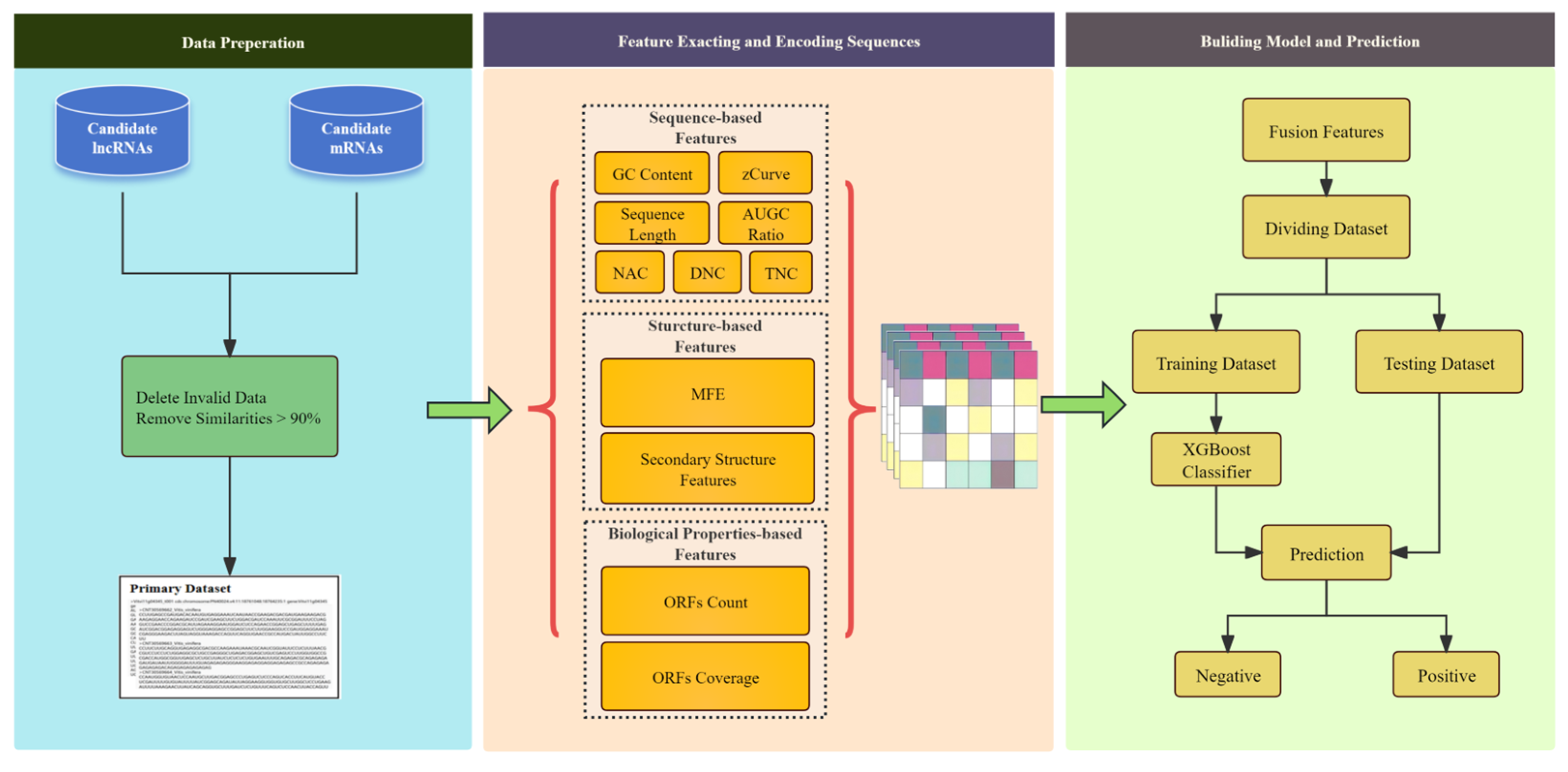
The overall framework of the LMFE consists of three steps. The first step involves the data preparation stage, where we obtained the lncRNA data as positive samples and the mRNA sequences as negative samples. In the second step, we focus on sequence representation and feature extraction, comprehensively capturing sequence features by considering the biological properties of RNA, sequence-based features, and structure-based features. Finally, we constructed an extreme gradient boosting (XGBoost) [
23] based on ensemble learning to predict lncRNAs.
Figure 1.
The overall framework of the LMFE consists of three steps. The first step involves the data preparation stage, where we obtained the lncRNA data as positive samples and the mRNA sequences as negative samples. In the second step, we focus on sequence representation and feature extraction, comprehensively capturing sequence features by considering the biological properties of RNA, sequence-based features, and structure-based features. Finally, we constructed an extreme gradient boosting (XGBoost) [
23] based on ensemble learning to predict lncRNAs.
Figure 2.
The comparison results between XGBoost and other methods. (A) The comparison of the ROC curves and AUC values of XGBoost and other methods. (B) The ACC compared with other mainstream methods; it can be observed that XGBoost achieves good performance, while GBDT, BG, and SVM are slightly better than other methods. (C) The time consumed by different classifiers on the training set. From the figure, it can be seen that SVM takes the longest time, while XGBoost’s advantage lies in its efficient performance.
Figure 3.
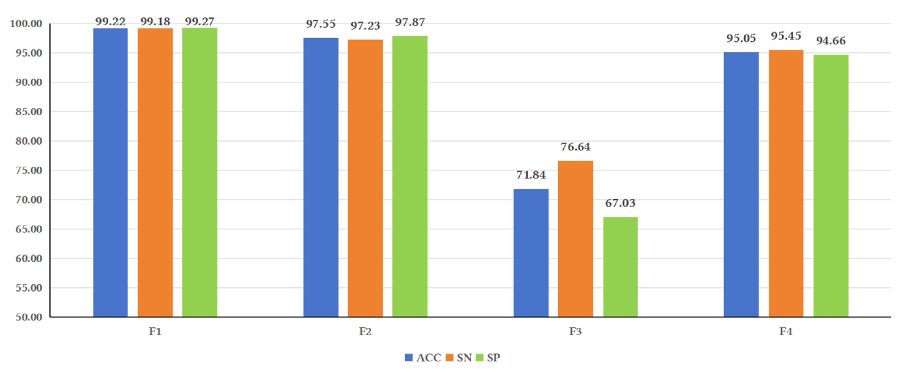
Illustrates the performance of the model under different feature fusions. Analysis of the evaluation metrics reveals that some metrics, such as ACC, SN, and SP, showed higher values for F1 compared to F2, F3, and F4. F2 yielded higher values than F3 and F4. These results indicate that sequence-based features have a significant impact on model performance. This could be attributed to studies that have observed the lack of secondary structure conservation in lncRNAs of certain species [
37], suggesting that secondary structure may not be as important for predicting lncRNAs as previously believed. These findings are consistent with the results of this study.
Figure 3.
Illustrates the performance of the model under different feature fusions. Analysis of the evaluation metrics reveals that some metrics, such as ACC, SN, and SP, showed higher values for F1 compared to F2, F3, and F4. F2 yielded higher values than F3 and F4. These results indicate that sequence-based features have a significant impact on model performance. This could be attributed to studies that have observed the lack of secondary structure conservation in lncRNAs of certain species [
37], suggesting that secondary structure may not be as important for predicting lncRNAs as previously believed. These findings are consistent with the results of this study.
Figure 4.
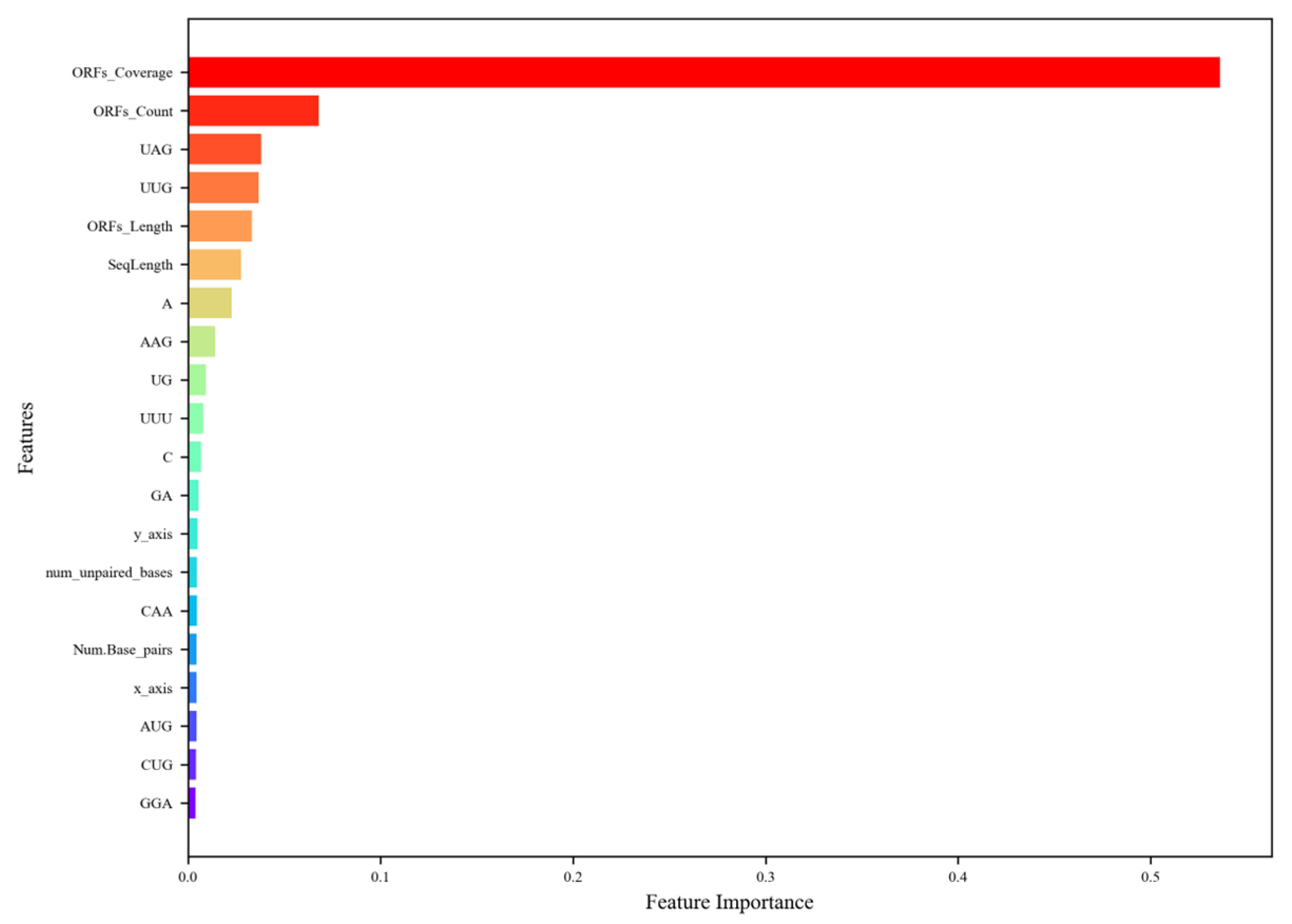
The ranking of the top 20 most important features. The descriptions of the feature abbreviations are as follows: ORFs_Coverage (ORF coverage), ORFs_Count (ORF count), ORFs_Length (ORF length), SeqLength (sequence length), y_axis (y asix), Num_unpaired_bases (the number of unpaired bases), Num_Base_pairs (the number of base pairs), and x_axis, (x axis). The figure highlights that ORF-related features dominate, with ORF coverage being the most significant, followed by ORF count and ORF length, reflecting their critical role in distinguishing lncRNAs from mRNAs due to the former’s lower ORF presence. Tri-nucleotide compositions, such as UAG and UUG, also rank highly, indicating their relevance in capturing sequence-level differences, particularly since stop codons, such as UAG, are more common in mRNAs. Sequence length and nucleotide compositions (e.g., A, C, GA) contribute moderately, while structural features (e.g., num_unpaired_bases, Num_Base_pairs) and Z-curve components (y_axis, x_axis) have lower importance (~0.03–0.04), suggesting that sequence-based features are more discriminatory than structural ones for lncRNA prediction in plants.
Figure 4.
The ranking of the top 20 most important features. The descriptions of the feature abbreviations are as follows: ORFs_Coverage (ORF coverage), ORFs_Count (ORF count), ORFs_Length (ORF length), SeqLength (sequence length), y_axis (y asix), Num_unpaired_bases (the number of unpaired bases), Num_Base_pairs (the number of base pairs), and x_axis, (x axis). The figure highlights that ORF-related features dominate, with ORF coverage being the most significant, followed by ORF count and ORF length, reflecting their critical role in distinguishing lncRNAs from mRNAs due to the former’s lower ORF presence. Tri-nucleotide compositions, such as UAG and UUG, also rank highly, indicating their relevance in capturing sequence-level differences, particularly since stop codons, such as UAG, are more common in mRNAs. Sequence length and nucleotide compositions (e.g., A, C, GA) contribute moderately, while structural features (e.g., num_unpaired_bases, Num_Base_pairs) and Z-curve components (y_axis, x_axis) have lower importance (~0.03–0.04), suggesting that sequence-based features are more discriminatory than structural ones for lncRNA prediction in plants.
![Genes 16 00424 g004]()
Figure 5.
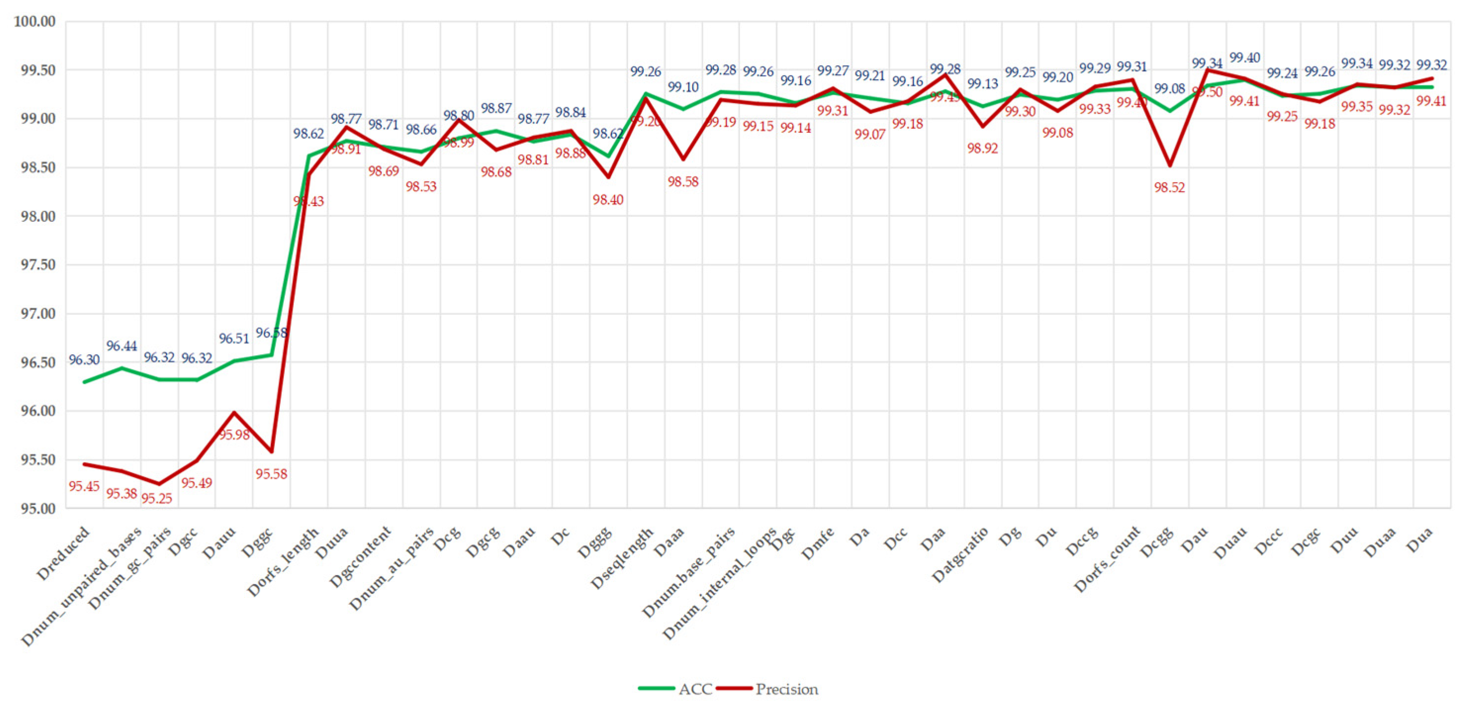
Illustrates that, with the reintroduction of redundant features, the ACC and precision metrics show an overall upward trend, increasing from 96.30% and 95.45% to 99.41% and 99.32%, respectively, with improvement rates of 3.11% and 3.87%. However, slight fluctuations were observed; for instance, adding “num_unpaired_bases” increased the ACC to 96.44%, while precision slightly decreased to 95.38%, indicating potential fluctuations due to its direct correlation with RNA structural stability. The most significant improvement occurred after the addition of “Dorfs_length”, with the ACC increasing from 95.58% to 98.43%, reflecting the crucial role of ORF-related features in distinguishing lncRNAs from mRNAs. However, with the addition of feature “C”, slight fluctuations in ACC and precision were noted, decreasing from 98.84% and 98.88% to 98.62% and 98.40%, respectively. This indicates that these features may introduce noise or overfitting to certain samples, possibly due to their high correlation with existing features, such as nucleotide composition. As the reintroduction process neared its conclusion, with the introduction of features, such as “Dgcc” and “Duaa”, both ACC and precision were restored. The ACC ultimately stabilized at 99.32% to 99.40%, with precision stabilizing at around 99.32% to 99.41%, nearing the performance of all features, which had 99.32% ACC and 99.41% precision. This analysis indicates that, although some redundant features (such as “Dnum_au_pairs”) temporarily compromise precision, the overall trend supports their inclusion in the complete feature set, as they collectively enhance LMFE’s ability to capture subtle patterns in RNA sequences, especially when balanced with biologically significant features, such as ORF coverage. These findings emphasize the robustness of XGBoost in processing relevant features and suggest that careful feature selection can alleviate transient performance degradation. We will further explore this consideration in future work by integrating advanced feature selection techniques.
Figure 5.
Illustrates that, with the reintroduction of redundant features, the ACC and precision metrics show an overall upward trend, increasing from 96.30% and 95.45% to 99.41% and 99.32%, respectively, with improvement rates of 3.11% and 3.87%. However, slight fluctuations were observed; for instance, adding “num_unpaired_bases” increased the ACC to 96.44%, while precision slightly decreased to 95.38%, indicating potential fluctuations due to its direct correlation with RNA structural stability. The most significant improvement occurred after the addition of “Dorfs_length”, with the ACC increasing from 95.58% to 98.43%, reflecting the crucial role of ORF-related features in distinguishing lncRNAs from mRNAs. However, with the addition of feature “C”, slight fluctuations in ACC and precision were noted, decreasing from 98.84% and 98.88% to 98.62% and 98.40%, respectively. This indicates that these features may introduce noise or overfitting to certain samples, possibly due to their high correlation with existing features, such as nucleotide composition. As the reintroduction process neared its conclusion, with the introduction of features, such as “Dgcc” and “Duaa”, both ACC and precision were restored. The ACC ultimately stabilized at 99.32% to 99.40%, with precision stabilizing at around 99.32% to 99.41%, nearing the performance of all features, which had 99.32% ACC and 99.41% precision. This analysis indicates that, although some redundant features (such as “Dnum_au_pairs”) temporarily compromise precision, the overall trend supports their inclusion in the complete feature set, as they collectively enhance LMFE’s ability to capture subtle patterns in RNA sequences, especially when balanced with biologically significant features, such as ORF coverage. These findings emphasize the robustness of XGBoost in processing relevant features and suggest that careful feature selection can alleviate transient performance degradation. We will further explore this consideration in future work by integrating advanced feature selection techniques.
![Genes 16 00424 g005]()
Figure 6.
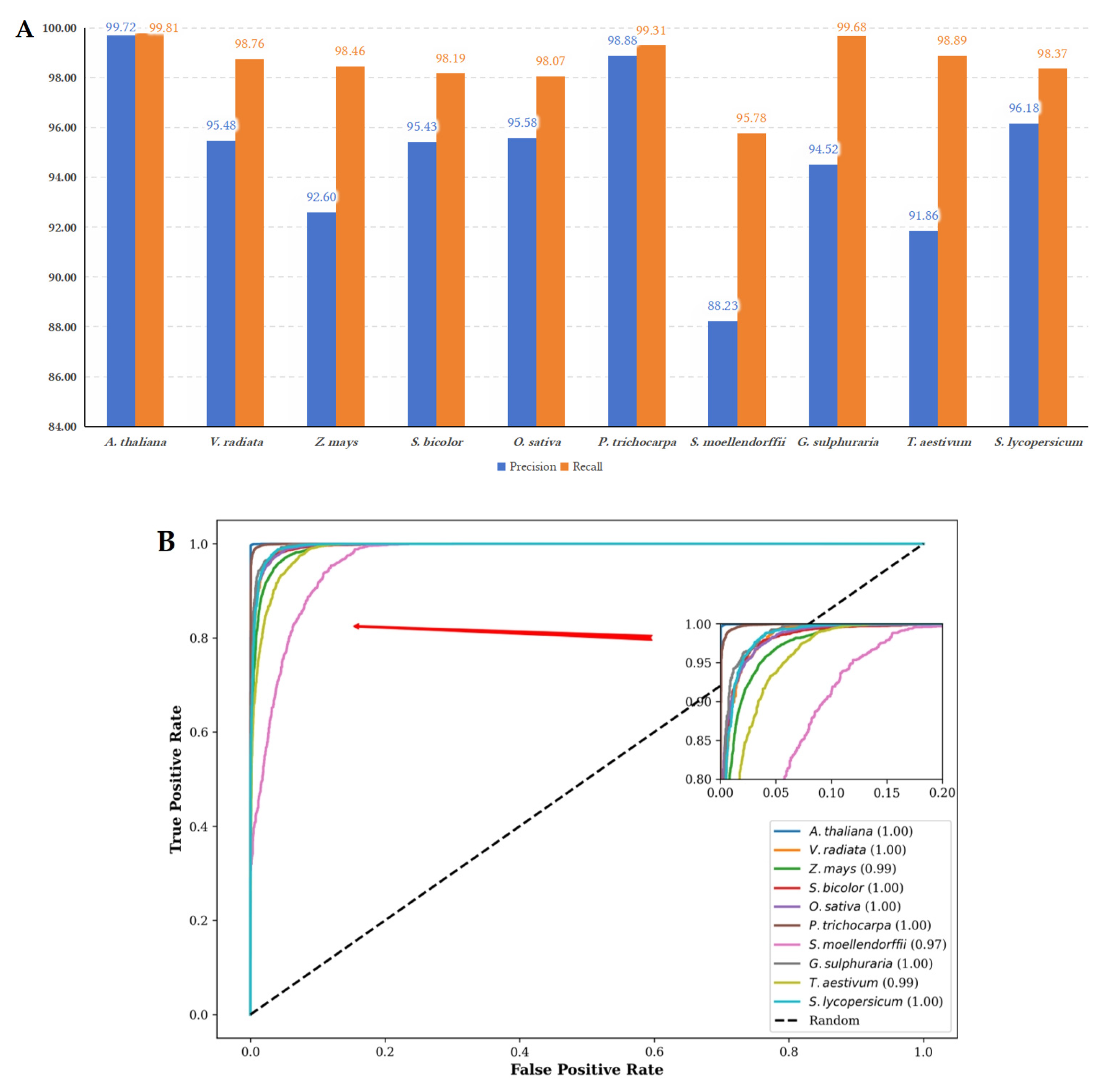
(A) The performance metrics of precision and recall for LMFE trained on the A. thaliana dataset and evaluated on other species. The LMFE demonstrates excellent performance on the A. thaliana dataset, with precision and recall values approaching 99.72% and 99.81%, respectively. This indicates a strong adaptability to the characteristics of the species. The verification results for other species reveal that the precision remains relatively stable, with a slight decrease observed in S. lycopersicum. The highest precision is recorded at 99.31% for P. trichocarpa, while the lowest precision is 88.23% for S. mollendorffii. In terms of recall, all species maintain values above 98%, with the highest recall at 99.68% for G. sulphuraria and the lowest recall at 95.78% for S. mollendorffii. Overall, LMFE exhibits a consistent trend in precision and recall across different species, with only minor fluctuations, suggesting its robustness and potential for broad applicability in various biological contexts. (B) The ROC curves for LMFE trained on the A. thaliana dataset and assessed across various species. The ROC curve serves as a graphical representation of performance, plotting the true positive rate against the false positive rate at various threshold settings. The ROC curve for A. thaliana is nearly perfect, signifying that LMFE excels at distinguishing positive samples with minimal false positives. The AUC value of 1.00 indicates that LMFE can correctly identify the majority of positive samples. Other species, such as V. radiata and Z. mays, also demonstrate strong performances, with AUC values of 1.00 and 0.99, respectively. This suggests that LMFE maintains a high level of accuracy for these species. However, the ROC curve for S. moellendorffii is comparatively lower, with an AUC value of 0.97. While still indicating good performance, this suggests that LMFE’s performance on this species is slightly less robust than on others, potentially due to differences in data characteristics. Overall, LMFE exhibits excellent training results on the A. thaliana dataset and demonstrates strong performance across different species.
Figure 6.
(A) The performance metrics of precision and recall for LMFE trained on the A. thaliana dataset and evaluated on other species. The LMFE demonstrates excellent performance on the A. thaliana dataset, with precision and recall values approaching 99.72% and 99.81%, respectively. This indicates a strong adaptability to the characteristics of the species. The verification results for other species reveal that the precision remains relatively stable, with a slight decrease observed in S. lycopersicum. The highest precision is recorded at 99.31% for P. trichocarpa, while the lowest precision is 88.23% for S. mollendorffii. In terms of recall, all species maintain values above 98%, with the highest recall at 99.68% for G. sulphuraria and the lowest recall at 95.78% for S. mollendorffii. Overall, LMFE exhibits a consistent trend in precision and recall across different species, with only minor fluctuations, suggesting its robustness and potential for broad applicability in various biological contexts. (B) The ROC curves for LMFE trained on the A. thaliana dataset and assessed across various species. The ROC curve serves as a graphical representation of performance, plotting the true positive rate against the false positive rate at various threshold settings. The ROC curve for A. thaliana is nearly perfect, signifying that LMFE excels at distinguishing positive samples with minimal false positives. The AUC value of 1.00 indicates that LMFE can correctly identify the majority of positive samples. Other species, such as V. radiata and Z. mays, also demonstrate strong performances, with AUC values of 1.00 and 0.99, respectively. This suggests that LMFE maintains a high level of accuracy for these species. However, the ROC curve for S. moellendorffii is comparatively lower, with an AUC value of 0.97. While still indicating good performance, this suggests that LMFE’s performance on this species is slightly less robust than on others, potentially due to differences in data characteristics. Overall, LMFE exhibits excellent training results on the A. thaliana dataset and demonstrates strong performance across different species.
![Genes 16 00424 g006]()
Figure 7.
The confusion matrix for LMFE’s performance on
G. max dataset after applying SMOTE, illustrating its ability to classify lncRNA and mRNA sequences. After SMOTE, the dataset was balanced to include 4000 true lncRNA samples and 4000 true mRNA samples. The matrix shows that out of 4000 true lncRNA samples, 3976 were correctly predicted as lncRNA (true positives), while 24 were misclassified as mRNA (false negatives). Conversely, out of 4000 true mRNA samples, 3947 were correctly predicted as mRNA (true negatives), but 53 were misclassified as lncRNA (false positives). The high values along the diagonal (3976 and 3947) and the low off-diagonal values (24 and 53) indicate a low error rate, demonstrating that LMFE accurately distinguishes between lncRNA and mRNA in most cases, with strong recognition ability for both categories despite the unbalanced dataset after applying SMOTE. Experimental results for other species are shown in
Figures S10–S12 in the Supplementary Materials.
Figure 8.
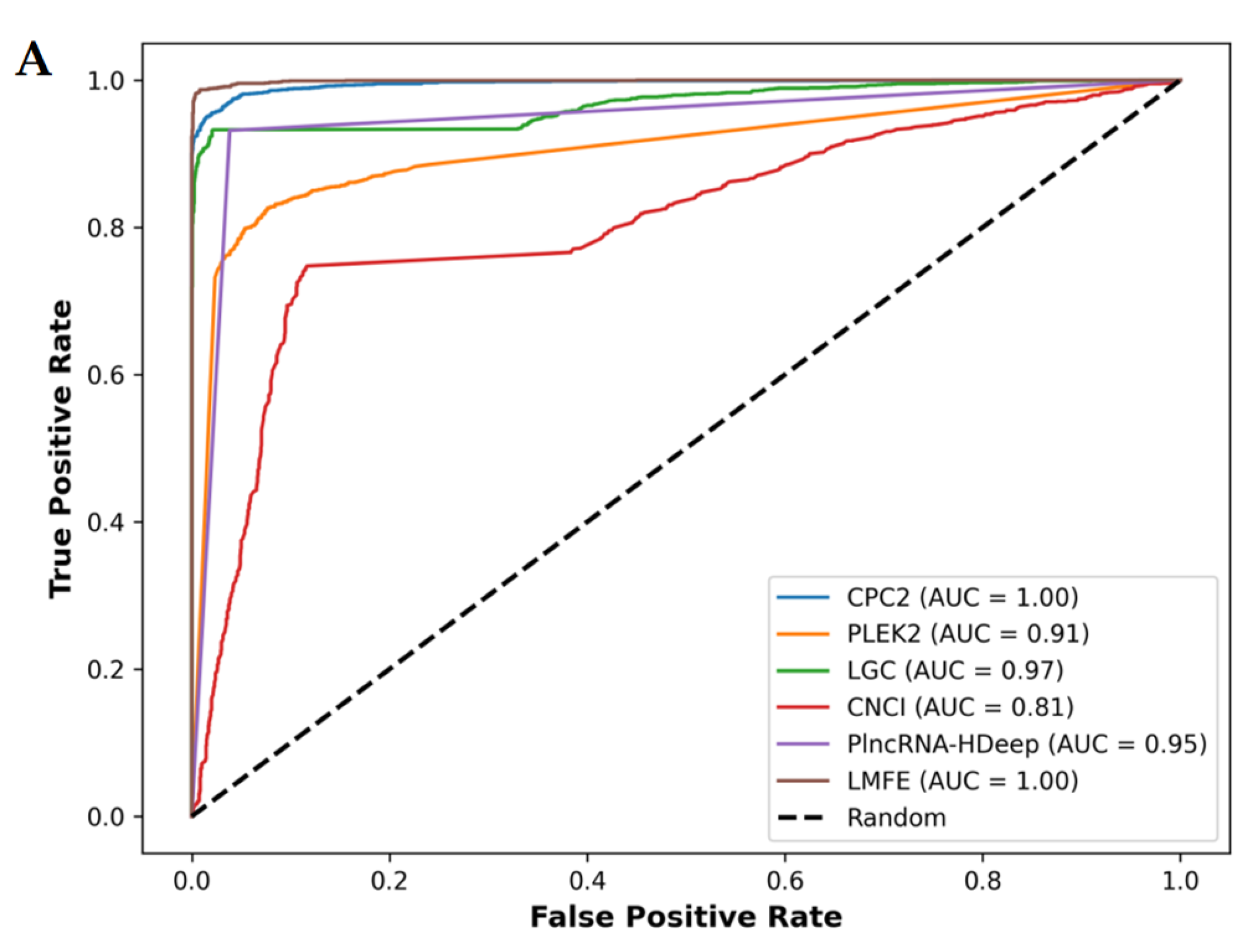
(A) Demonstrates that in the V. angularis, the AUC value of LMFE is 1.00, indicating excellent performance in distinguishing positive and negative samples, achieving perfect true positive rates at nearly all thresholds. CPC2, LGC, and PlncRNA-Hdeep also show perfect capabilities. In contrast, CNCI obtained a slightly lower AUC value of 0.87. (B) Confirms that LMFE demonstrated superior performance across all metrics, achieving a score of 0.99, reflecting extremely high accuracy and comprehensiveness. LGC and CPC2 closely followed, with a precision of 0.99 and recall and F1scores of 0.93 and 0.96, respectively, indicating a good balance. PlncRNA-Hdeep achieved a precision of 0.96, recall of 0.93, and F1score of 0.95, showcasing its effectiveness. PLEKv2 achieved a precision of 0.91, recall of 0.83, and F1score of 0.87; its low recall suggests that its ability to identify positive samples requires optimization. Conversely, CNCI exhibited the poorest performance, with a precision of 0.87, recall of only 0.75, and F1score of 0.80, indicating significant deficiencies in identifying positive samples.
Figure 8.
(A) Demonstrates that in the V. angularis, the AUC value of LMFE is 1.00, indicating excellent performance in distinguishing positive and negative samples, achieving perfect true positive rates at nearly all thresholds. CPC2, LGC, and PlncRNA-Hdeep also show perfect capabilities. In contrast, CNCI obtained a slightly lower AUC value of 0.87. (B) Confirms that LMFE demonstrated superior performance across all metrics, achieving a score of 0.99, reflecting extremely high accuracy and comprehensiveness. LGC and CPC2 closely followed, with a precision of 0.99 and recall and F1scores of 0.93 and 0.96, respectively, indicating a good balance. PlncRNA-Hdeep achieved a precision of 0.96, recall of 0.93, and F1score of 0.95, showcasing its effectiveness. PLEKv2 achieved a precision of 0.91, recall of 0.83, and F1score of 0.87; its low recall suggests that its ability to identify positive samples requires optimization. Conversely, CNCI exhibited the poorest performance, with a precision of 0.87, recall of only 0.75, and F1score of 0.80, indicating significant deficiencies in identifying positive samples.
![Genes 16 00424 g008a]()
![Genes 16 00424 g008b]()
Table 1.
Benchmark dataset.
Table 1.
Benchmark dataset.
| Species | Dataset | Total |
|---|
| Positive Data | Negative Data |
|---|
| A. thaliana | 6775 | 6775 | 13,550 |
| V. radiata | 4600 | 4600 | 9200 |
| Z. mays | 11,572 | 11,572 | 23,144 |
| S. bicolor | 5400 | 5400 | 10,800 |
| O. sativa | 6003 | 6003 | 12,006 |
| P. trichocarpa | 5615 | 5615 | 11,230 |
| S. moellendorffii | 2300 | 2300 | 4600 |
| G. sulphuraria | 1870 | 1870 | 3740 |
| T. aestivum | 6500 | 6500 | 13,000 |
| S. lycopersicum | 3377 | 3377 | 6754 |
Table 2.
Independent testing dataset.
Table 2.
Independent testing dataset.
| Species | Dataset | Total |
|---|
| Positive Data | Negative Data |
|---|
| V. angularis | 2000 | 2000 | 4000 |
| S. indicum | 3400 | 3400 | 6800 |
| B. distachyon | 3000 | 3000 | 6000 |
| M. acuminata | 5600 | 5600 | 11,200 |
| M. polymorpha | 1200 | 1200 | 2400 |
| N. colorata | 2100 | 2100 | 4200 |
Table 3.
Unbalanced dataset.
Table 3.
Unbalanced dataset.
| Species | Dataset | Total |
|---|
| Positive Data | Negative Data |
|---|
| G. max | 4000 | 2000 | 6000 |
| M. domestica | 2000 | 5500 | 7500 |
| A. officinalis | 6500 | 2300 | 8800 |
| L. angustifolius | 1700 | 4800 | 6500 |
Table 4.
Feature extraction methods.
Table 4.
Feature extraction methods.
| Classification | Method | Number of Features |
|---|
| Biological properties-based method | ORF count | 1 |
| ORF coverage | 1 |
| ORF length | 1 |
| Sequence-based method | Sequence length | 1 |
| GC content | 1 |
| Z-curve | 3 |
| AUGC ratio | 1 |
| NAC | 4 |
| DNC | 16 |
| TNC | 64 |
| Structure-based method | SS | 6 |
| MFE | 1 |
| Total | | 100 |
Table 5.
Performance of LMFE on the benchmark dataset.
Table 5.
Performance of LMFE on the benchmark dataset.
| Dataset | ACC (%) | SN (%) | SP (%) | F1score | MCC |
|---|
| Benchmark dataset | 99.42 | 99.36 | 99.48 | 0.99 | 0.98 |
Table 6.
Comparison Between XGBoost and other methods.
Table 6.
Comparison Between XGBoost and other methods.
| Method | ACC (%) | SN (%) | SP (%) | F1score | MCC |
|---|
| KNN | 88.74 | 85.08 | 92.40 | 0.88 | 0.78 |
| DT | 97.24 | 97.27 | 97.22 | 0.97 | 0.94 |
| NB | 81.24 | 76.63 | 85.85 | 0.80 | 0.63 |
| SVM | 98.20 | 99.00 | 97.40 | 0.98 | 0.96 |
| BG | 98.41 | 98.14 | 98.68 | 0.98 | 0.97 |
| RF | 97.61 | 98.72 | 96.50 | 0.98 | 0.95 |
| AB | 97.56 | 97.96 | 97.16 | 0.98 | 0.95 |
| GBDT | 98.59 | 98.74 | 98.44 | 0.99 | 0.97 |
| XGBoost | 99.36 | 99.31 | 99.41 | 0.99 | 0.99 |
Table 7.
The performance of LMFE on the benchmark dataset.
Table 7.
The performance of LMFE on the benchmark dataset.
| Training Species | Metrics | Testing Species |
|---|
| A. thaliana | V. radiata | Z. mays | S. bicolor | O. sativa | P. trichocarpa | S. moellendorffii | G. sulphuraria | T. aestivum | S. lycopersicum |
|---|
| A. thaliana | ACC (%) | 99.76 | 97.04 | 95.30 | 96.74 | 96.77 | 99.09 | 91.50 | 96.95 | 95.06 | 97.23 |
| SN (%) | 99.81 | 98.76 | 98.46 | 98.19 | 98.07 | 99.31 | 95.78 | 99.68 | 98.89 | 98.37 |
| SP (%) | 99.72 | 95.33 | 92.13 | 95.30 | 95.48 | 98.88 | 87.22 | 94.23 | 91.23 | 96.09 |
| F1score | 1.00 | 0.97 | 0.95 | 0.97 | 0.97 | 0.99 | 0.92 | 0.97 | 0.95 | 0.97 |
| MCC | 1.00 | 0.94 | 0.91 | 0.94 | 0.94 | 0.98 | 0.83 | 0.94 | 0.90 | 0.95 |
| V. radiata | ACC (%) | 98.12 | 99.57 | 94.96 | 95.08 | 95.74 | 98.46 | 92.87 | 97.19 | 94.98 | 97.65 |
| SN (%) | 99.01 | 99.67 | 98.79 | 98.52 | 98.58 | 99.29 | 96.09 | 99.63 | 99.09 | 98.67 |
| SP (%) | 97.23 | 99.46 | 91.13 | 91.65 | 92.90 | 97.63 | 89.65 | 94.76 | 90.86 | 96.62 |
| F1score | 0.98 | 1.00 | 0.95 | 0.95 | 0.96 | 0.99 | 0.93 | 0.97 | 0.95 | 0.98 |
| MCC | 0.96 | 0.99 | 0.90 | 0.90 | 0.92 | 0.97 | 0.86 | 0.95 | 0.90 | 0.95 |
| Z. mays | ACC (%) | 98.89 | 97.58 | 99.61 | 97.90 | 98.09 | 98.84 | 95.61 | 97.06 | 95.04 | 98.28 |
| SN (%) | 98.51 | 98.09 | 99.59 | 97.96 | 98.78 | 98.38 | 96.22 | 99.14 | 98.08 | 98.05 |
| SP (%) | 99.26 | 97.07 | 99.62 | 97.83 | 97.39 | 99.31 | 95.00 | 94.97 | 92.00 | 98.52 |
| F1score | 0.99 | 0.98 | 1.00 | 0.98 | 0.98 | 0.99 | 0.96 | 0.97 | 0.95 | 0.98 |
| MCC | 0.98 | 0.95 | 0.99 | 0.96 | 0.96 | 0.98 | 0.91 | 0.94 | 0.90 | 0.97 |
| S. bicolor | ACC (%) | 98.75 | 97.74 | 96.51 | 99.66 | 98.54 | 98.83 | 93.09 | 97.70 | 96.04 | 97.59 |
| SN (%) | 98.86 | 98.41 | 98.36 | 99.72 | 99.00 | 98.75 | 96.65 | 99.47 | 98.63 | 97.99 |
| SP (%) | 98.64 | 97.07 | 94.67 | 99.59 | 98.07 | 98.91 | 89.52 | 95.94 | 93.45 | 97.19 |
| F1score | 0.99 | 0.98 | 0.97 | 1.00 | 0.99 | 0.99 | 0.93 | 0.98 | 0.96 | 0.98 |
| MCC | 0.98 | 0.96 | 0.93 | 0.99 | 0.97 | 0.98 | 0.86 | 0.96 | 0.92 | 0.95 |
| O. sativa | ACC (%) | 98.60 | 98.14 | 96.16 | 97.72 | 99.78 | 98.49 | 91.98 | 97.62 | 96.15 | 97.57 |
| SN (%) | 98.95 | 98.48 | 98.36 | 98.19 | 99.75 | 98.72 | 96.26 | 99.25 | 98.43 | 98.05 |
| SP (%) | 98.24 | 97.80 | 93.97 | 97.26 | 99.80 | 98.26 | 87.70 | 95.99 | 93.88 | 97.10 |
| F1score | 0.99 | 0.98 | 0.96 | 0.98 | 1.00 | 0.99 | 0.92 | 0.98 | 0.96 | 0.98 |
| MCC | 0.97 | 0.96 | 0.92 | 0.95 | 1.00 | 0.97 | 0.84 | 0.95 | 0.92 | 0.95 |
| P. trichocarpa | ACC (%) | 98.78 | 97.15 | 95.55 | 97.03 | 96.94 | 99.81 | 90.80 | 97.49 | 95.47 | 97.16 |
| SN (%) | 98.38 | 98.15 | 97.68 | 97.46 | 97.05 | 99.79 | 93.22 | 99.36 | 98.45 | 97.69 |
| SP (%) | 99.19 | 96.15 | 93.42 | 96.59 | 96.82 | 99.84 | 88.39 | 95.62 | 92.49 | 96.62 |
| F1score | 0.99 | 0.97 | 0.96 | 0.97 | 0.97 | 1.00 | 0.91 | 0.98 | 0.96 | 0.97 |
| MCC | 0.98 | 0.94 | 0.91 | 0.94 | 0.94 | 1.00 | 0.82 | 0.95 | 0.91 | 0.94 |
| S. moellendorffii | ACC (%) | 97.68 | 97.10 | 96.38 | 95.39 | 96.24 | 96.92 | 99.09 | 95.00 | 94.03 | 95.62 |
| SN (%) | 98.95 | 98.26 | 98.67 | 98.22 | 98.77 | 98.65 | 99.48 | 98.45 | 98.25 | 97.34 |
| SP (%) | 96.40 | 95.94 | 94.10 | 92.56 | 93.71 | 95.19 | 98.70 | 91.55 | 89.82 | 93.90 |
| F1score | 0.98 | 0.97 | 0.97 | 0.96 | 0.96 | 0.97 | 0.99 | 0.95 | 0.94 | 0.96 |
| MCC | 0.95 | 0.94 | 0.93 | 0.91 | 0.93 | 0.94 | 0.98 | 0.90 | 0.88 | 0.91 |
| G. sulphuraria | ACC (%) | 96.58 | 96.61 | 94.47 | 94.25 | 95.68 | 97.13 | 89.30 | 99.41 | 94.92 | 94.86 |
| SN (%) | 95.97 | 95.94 | 96.02 | 94.37 | 95.14 | 96.90 | 89.78 | 99.57 | 96.22 | 94.70 |
| SP (%) | 97.18 | 97.28 | 92.92 | 94.13 | 96.22 | 97.36 | 88.83 | 99.25 | 93.62 | 95.03 |
| F1score | 0.97 | 0.97 | 0.95 | 0.94 | 0.96 | 0.97 | 0.89 | 0.99 | 0.95 | 0.95 |
| MCC | 0.93 | 0.93 | 0.89 | 0.89 | 0.91 | 0.94 | 0.79 | 0.99 | 0.90 | 0.90 |
| T. aestivum | ACC (%) | 97.71 | 97.42 | 93.83 | 95.94 | 97.32 | 97.77 | 90.70 | 98.48 | 99.75 | 97.01 |
| SN (%) | 98.38 | 97.39 | 98.07 | 97.91 | 98.37 | 98.70 | 93.30 | 99.04 | 99.72 | 97.75 |
| SP (%) | 97.03 | 97.46 | 89.58 | 93.96 | 96.27 | 96.85 | 88.09 | 97.91 | 99.79 | 96.27 |
| F1score | 0.98 | 0.97 | 0.94 | 0.96 | 0.97 | 0.98 | 0.91 | 0.99 | 1.00 | 0.97 |
| MCC | 0.95 | 0.95 | 0.88 | 0.92 | 0.95 | 0.96 | 0.82 | 0.97 | 1.00 | 0.94 |
| S. lycopersicum | ACC (%) | 98.57 | 97.80 | 96.23 | 97.08 | 97.35 | 98.63 | 94.30 | 97.06 | 95.76 | 99.53 |
| SN (%) | 98.63 | 98.74 | 98.13 | 97.46 | 98.75 | 98.63 | 95.78 | 99.23 | 99.15 | 99.44 |
| SP (%) | 98.51 | 96.87 | 94.34 | 96.70 | 95.96 | 98.63 | 92.83 | 94.39 | 92.37 | 99.62 |
| F1score | 0.99 | 0.98 | 0.96 | 0.97 | 0.97 | 0.99 | 0.94 | 0.97 | 0.96 | 1.00 |
| MCC | 0.97 | 0.96 | 0.93 | 0.94 | 0.95 | 0.97 | 0.89 | 0.94 | 0.92 | 0.99 |
Table 8.
The performance of LMFE on unbalanced datasets.
Table 8.
The performance of LMFE on unbalanced datasets.
| Species | ACC (%) | Recall (%) | F1score |
|---|
| EXP NO-SMOTE | EXP WITH-SMOTE | EXP NO-SMOTE | EXP WITH-SMOTE | EXP NO-SMOTE | EXP WITH-SMOTE |
|---|
| G. max | 95.66 | 99.04 | 93.56 | 99.40 | 0.97 | 0.99 |
| M. domestica | 79.84 | 99.62 | 100.00 | 99.84 | 0.73 | 1.00 |
| A. officinalis | 90.22 | 99.50 | 86.77 | 99.26 | 0.93 | 1.00 |
| L. angustifolius | 82.75 | 99.46 | 100.00 | 99.02 | 0.75 | 1.00 |
Table 9.
The performance comparison between LMFE and state-of-the-art methods.
Table 9.
The performance comparison between LMFE and state-of-the-art methods.
| Species | CPC2 | PLEKv2 | LGC | CNCI | PlncRNA-HDeep | LMFE |
|---|
| V. angularis | 96.20 | 87.22 | 96.05 | 81.55 | 94.63 | 98.85 |
| S. indicum | 96.06 | 88.37 | 94.53 | 85.78 | 99.12 | 98.69 |
| B. distachyon | 94.58 | 85.75 | 93.95 | 84.72 | 96.33 | 99.05 |
| M. acuminata | 96.85 | 89.04 | 95.71 | 85.79 | 99.60 | 99.00 |
| M. polymorpha | 92.63 | 86.67 | 92.63 | 78.87 | 76.88 | 99.21 |
| N. colorata | 91.64 | 85.98 | 88.71 | 76.64 | 94.40 | 97.33 |


