Article

Graph Node Classification to Predict Autism Risk in Genes

Department of Computer Science and Engineering, Fairfield University, Fairfield, CT 06824, USA
*
Author to whom correspondence should be addressed.
Genes 2024, 15(4), 447; https://doi.org/10.3390/genes15040447
Submission received: 20 February 2024 / Revised: 28 March 2024 / Accepted: 28 March 2024 / Published: 1 April 2024
(This article belongs to the Section Human Genomics and Genetic Diseases)

Abstract

:
This study explores the genetic risk associations with autism spectrum disorder (ASD) using graph neural networks (GNNs), leveraging the Sfari dataset and protein interaction network (PIN) data. We built a gene network with genes as nodes, chromosome band location as node features, and gene interactions as edges. Graph models were employed to classify the autism risk associated with newly introduced genes (test set). Three classification tasks were undertaken to test the ability of our models: binary risk association, multi-class risk association, and syndromic gene association. We tested graph convolutional networks, Graph Sage, graph transformer, and Multi-Layer Perceptron (Baseline) architectures on this problem. The Graph Sage model consistently outperformed the other models, showcasing its utility in classifying ASD-related genes. Our ablation studies show that the chromosome band location and protein interactions contain useful information for this problem. The models achieved 85.80% accuracy on the binary risk classification, 81.68% accuracy on the multi-class risk classification, and 90.22% on the syndromic classification.

1. Introduction

Autism spectrum disorder (ASD) is a deficit of social communication or sensory-motor function based on genetic association and other causations [1]. The genetic association is supported by the inheritance rate observed by Tick et al.’s [2] meta-data analysis on twins, which determined the inheritance of ASD to range between 64 and 91 percent. Tick et al. also associated a 0.98 correlation between genetics and neurodevelopmental disorders. De novo mutations further express the relationship inheritance has on ASD because these genetic mutations happen specifically with stem cell divisions and maturation of the female gametes within the trio (father, mother, and child) [3]. These genetic mutations are based on mutations found between the trio, determining the de novo mutation that carries the high inheritance seen within the Tick et al. analysis [4,5,6].
In the Handbook of Clinical Neurology [7], ASD connection is associated with an estimated 1000 genes determined based on genetic linkage between chromosome location (loci) and possible genetic risk. Alarcón et al. [8] performed a comprehensive study on chromosome regions 7q and 17q, finding that region 7q2-35 has a strong possibility of associating with ASD while also noting that other areas, like chromosome 3q, might also have an association with ASD. Copy number variants (CNV) is the process of adding, removing, or copying portions of deoxyribonucleic acid (DNA) [9]. CNV shows the exact genetic correlation on specific regions of the chromosome band, further exemplifying the link between loci and ASD.
Another genetic association is a common variant which significantly affects ASD risk. Grove et al. [10] used a genome-wide association study that determined common variants’ strong, robust connection with ASD. Common variants are significant factors in most diseases, as they relate to 90 percent of the differences between individuals [11]. From an individual perspective, common variants create minimal significance, but by putting all the variants together, we determine a noticeable impact for risk [12]. Common variants make up 40–60 percent of the risk factor when evaluating ASD [13].
Between all of the variants and genetic mutations, we see that these mutations and variants are connected within a network. Kolchanov et al. describe gene networks as a group of genes functioning in a coordinated manner [14]. As seen, common variants, de novo variants, and CNV are all the byproducts of genes functioning in coordination with one another, and that function creates variants with high ASD risk. These variants all combined create a gene network that links all of these variants together, showing us the association/non-association of a gene [15]. Graph neural networks have recently been proposed to address classic yet challenging graph problems, such as node or graph classification, and have been used for graph structure learning and graph classification. The diverse applications of GNNs in these studies underscore their broad utility in addressing various problems across various domains, including social networks, healthcare, and other network structures [16,17,18,19]. Our proposed experiment uses these gene networks and graph neural networks to determine if a gene has an association and the level of risk associated with the gene. The specific graph neural network models we use are Nodeformer [20], Graph Sage [21], and graph convolutional network (GCN) [22]. Within this experiment, we will use a binary and multi-class classifier to predict the likelihood of a gene being associated with autism risk. We will also use another binary classification approach to predict whether a gene is associated with a particular syndrome related to ASD. In addition, we conduct extensive experiments to determine the effect of gene location and gene network information on the classification.

2. Related Works

Genome-wide association study (GWAS) is a method used to find genetic variants that are associated with a particular disease or trait. It does this by comparing the DNA of people with the disease or trait to the DNA of people who do not have the disease or trait. Bralten et al. [23] used GWAS to find a connection between genetic sharing between ASDs and the autistic traits ‘childhood behavior’, ‘rigidity’, and ‘attention to detail’. Grove et al. [24] used this technique to find five genome-wide significant loci associated with autism risk. Krishnan et al. [25] developed a machine learning approach based on a human brain-specific gene network to present a genome-wide prediction of autism risk genes, including hundreds of candidates for which there is minimal or no prior genetic evidence. Rahman et al. (2020) [26] established a network known as a brain tissue-specific Functional Relational Network (FRN), which applies machine learning techniques to predict the genomic-activated autism-related genes. Furthermore, Ismail et al. (2022) [27] proposed a hybrid ensemble-based classification model for predicting ASD genes using machine learning. Lin et al. [28] employed a machine learning-based approach to predict ASD genes using features from spatiotemporal gene expression patterns in the human brain, gene-level constraint metrics, and other gene variation features. Furthermore, Brueggeman et al. [29] utilized machine learning and genome-scale data to forecast autism gene discovery.
Genes that confer risk for ASD are likely to be functionally related, thus converging on molecular networks and biological pathways implicated in disease [30]. Taking this idea further, Krumm et al. [31] showed that ASD genes with de novo mutations converged on pathways related to chromatin remodeling and synaptic function. Some later studies showed that integrating known risk genes using a protein–protein interaction (PPI) network can identify novel genes involved in ASD [32,33]. In this paper, we are analyzing the risk assessment using binary risk association labels, multi-class risk association labels (based on a score of confidence), and binary syndromic association for whether the gene is associated with an overarching medical condition.

Use of Graph Neural Networks to Predict Disease

In machine learning, many techniques have been used to predict diseases using gene networks, risk assessment ASD, and overall disease risk discovery using machine learning techniques. The first is the interaction discovery made in protein–protein interaction networks by Fenq et. al, who discovered using omic data that they can determine new links with these interaction networks [34]. Wang et al. used attention-based graph neural networks to identify ASD based on the activity within brain scans [35]. Beyreli et al. created DeepND, a multitask graph convolutional network that used an autism network and an intellectual disability network to determine the risk for both [36]. They achieved a median AUC of 87%. Lu et al. used a graph neural network and a patient network to classify whether a patient suffers from a chronic illness or not [37]. Wang and Avillach used DeepAutism, a convolutional network designed to diagnose ASD based on the presence of high-risk gene variants [38]. They achieved 88.6% accuracy. Motsinger et al. used gene–gene interaction networks and neural networks to classify the risk people carry for Parkinson’s disease [39]. Laksshman et al. created deep bipolar, which specializes in identifying gene mutations to determine whether somebody is bipolar [40].

3. Methodology

3.1. Dataset

The datasets used for these experiments were the Sfari dataset [41] and protein interaction network (PIN) data [15]. The Sfari dataset contains gene associations and rankings (labels). It also contains the chromosome band location of each specific gene. For our binary risk association and multi-class risk association classification, we used the confidence score on Sfari, which ranks from most confident to least confident association in ASD (ranking from 1 to 3).
  • Case (1) Binary risk association classification. If a gene is contained in the SFARI dataset, it is automatically considered to contain risk for ASD. The two classes for this are as follows:
    1
    Gene with associated risk;
    2
    Gene without associated risk.
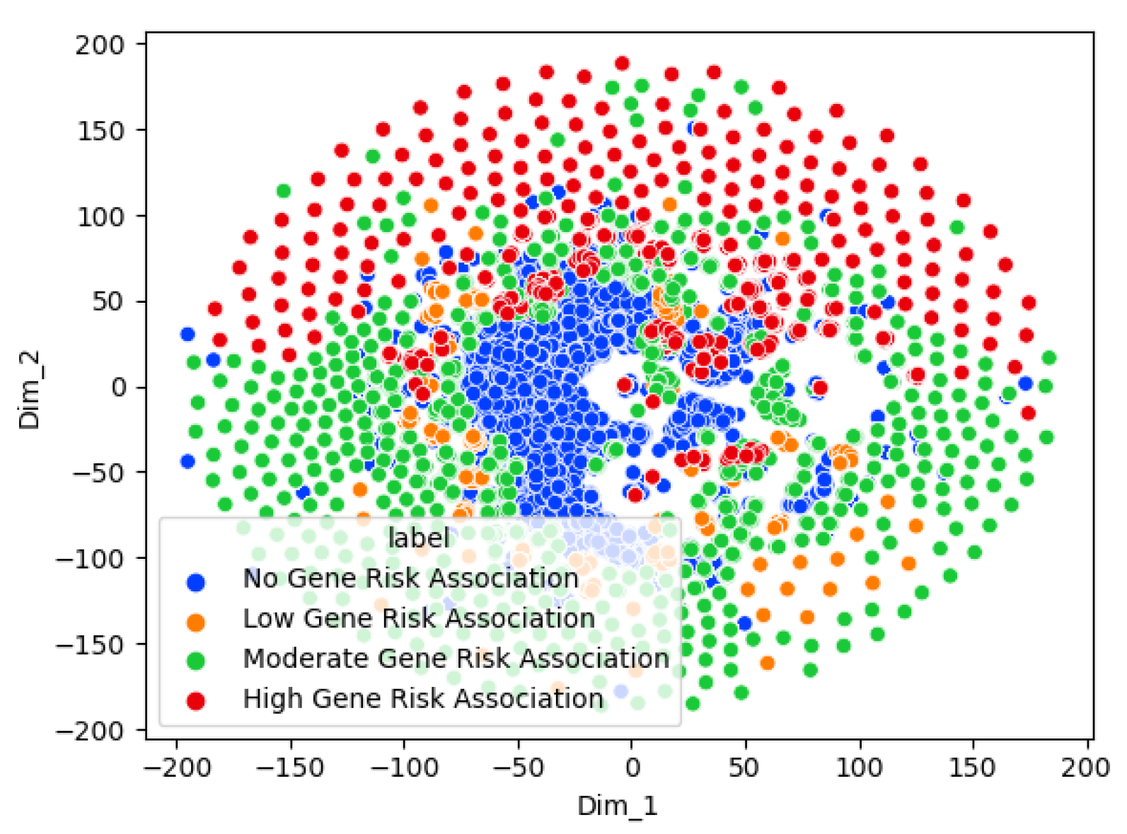
  • Case (2) The multi-class risk association classification uses three risk levels for its labels. The classes for this classification are as follows:
    1
    No gene association;
    2
    Low gene association;
    3
    Moderate gene association;
    4
    High gene association.
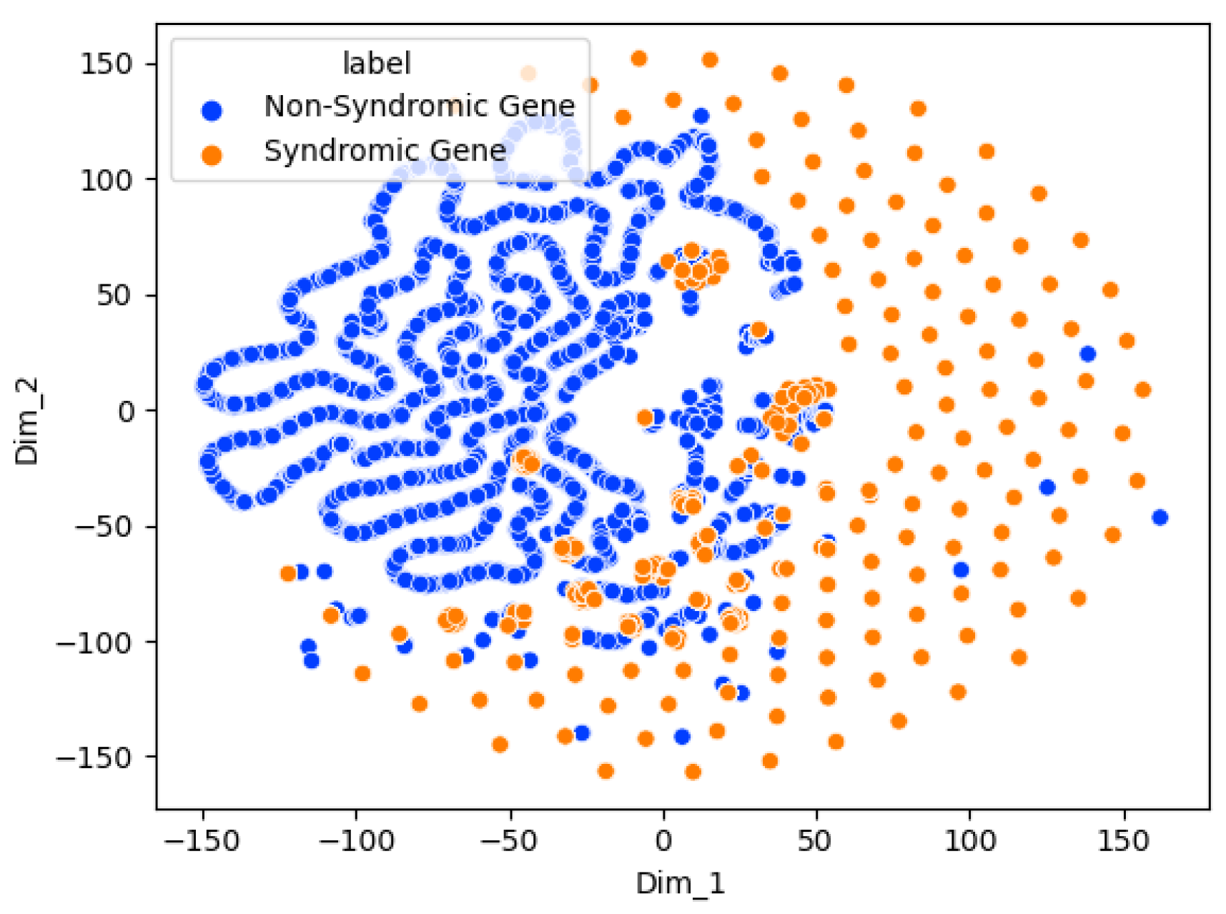
  • Case (3) Syndromic gene classification. (Syndromes are collections of multiple, related medical signs and symptoms that occur together. Mutations in a syndromic gene can lead to a variety of problems affecting different parts of the body and causing a recognizable pattern of symptoms.) The syndromic risk association shows us the identification of syndromic and possible non-syndromic genes. (Sfari dataset lists all specifically syndromic gene associations). The classes are as follows:
    1
    Syndromic gene;
    2
    Non-syndromic gene.
The PIN dataset comprises data on protein–protein interactions, elucidating which proteins interact. These interactions can be represented as a network or graph, where proteins are nodes, and interactions between them are edges or connections. The PIN dataset contains all protein–protein interactions both associated and not associated with ASD.

3.2. Preprocessing

The first preprocessing step is to filter out anything in the PIN dataset that is not specified as being a human gene interaction. Next, we add the chromosome band location and labels (binary, multi-class, and syndromic) from the Sfari dataset to the genes in the PIN dataset to have our edges and associated labels. The chromosome band locations obtained from the Sfari dataset are used as node features. Equation (1) shows the definition of the graph:
G = ( V , E , C )
  • G: The graph representing genes and their interactions.
  • V: The set of nodes, where each node represents a gene and is associated with its location (feature).
  • E: The set of edges representing interactions or connections between genes in the graph.
  • C: The set of labels representing autism risk for each gene, where each gene node is associated with a label indicating its classification (high confidence, strong candidate, suggestive evidence).
The chromosome band is placed in a one-hot encoder that splits our feature into a list of 472 binary features representing every possible location where the gene has been observed. This is then also followed up with using our edge list to create an adjacency matrix and then passing our labels. In the case of multi-class classification, the high confidence class contains 214 genes, the strong candidate class includes 530 genes, and the suggestive evidence class has 69 genes. This is paired with 11,403 no associated genes, which shows a severe imbalance. To fix this imbalance, we upsample [42] all of the genes to ensure we have a balanced classification among all four classes. For the binary class, we take the high confidence class, strong candidate class, and the suggestive evidence class together, which is 813 genes with the same paired 114,03 non associated genes. Lastly, the syndromic labels are split into 169 syndromic genes and 12,047 that are not syndromic. The preprocessing steps are visualized in Figure 1.

3.3. Models

The models used for this experiment are graph convolutional network [22], Graph Sage [
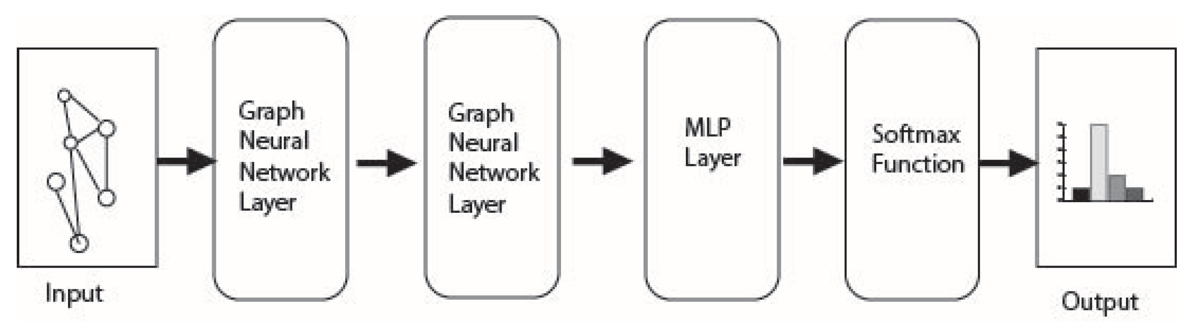
21], and Multi-Layer Perceptron (MLP). The models each contain two layers, each having a rectified linear unit (ReLu) between the layers and ending with a multilayer perceptron (MLP). These models are set up to use the adjacency matrix, feature matrix, and selected labels to create either a binary or multi-class classification.

3.4. Graph Convolutional Network

GCN uses the convolutional properties of a graph network to facilitate a connection of both the features and the network. This process is performed in a layer of the GCN called the propagation Layer (Equation (2)), where l is the layer of the GCN operation; h v ( l ) is the feature vector of node v in the l-th layer; N ( v ) is the set of neighboring nodes of node v; W ( l ) is the weight matrix for the l-th layer; c v is a normalization factor for node v; and σ is an activation function (e.g., ReLU):
h v ( l + 1 ) = σ u N ( v ) 1 c v W ( l ) h u ( l )
GCN is more of a top-down approach, which looks at the entire picture of the network and its feature matrix for performing calculations. This model ignores the effect a singular node has on the network but instead looks at all of the interactions together through matrix multiplication. Once this is done, we obtain our embedding matrix, allowing us to classify what class a node belongs to.

3.5. Graph Sage

Graph Sage takes an aggregation of all neighboring nodes in the network. The Graph Sage operation is defined in Equation (3), where l is the layer of the GraphSAGE operation; h v ( l ) is the feature vector of node v in the l-th layer; N ( v ) is the set of neighboring nodes of node v; W ( l ) is the weight matrix for the l-th layer; A G G R E G A T E is the aggregation function (e.g., mean, sum, or LSTM-based aggregation); and σ is the activation function (e.g., ReLU):
h v ( l + 1 ) = σ W ( l ) · AGGREGATE ( h u ( l ) , u N ( v ) )
Mean aggregated features are then concatenated to create new features for every node in the feature matrix. This model infers the connection of neighboring nodes. This connection creates another approach but an essential method for interpreting graph networks. Instead of using a broad look like GCN, this takes a neighboring approach, which instead infers the connection a feature relationship that not only the current node but its neighboring nodes have with each other.

3.6. Graph Transformer (Nodeformer)
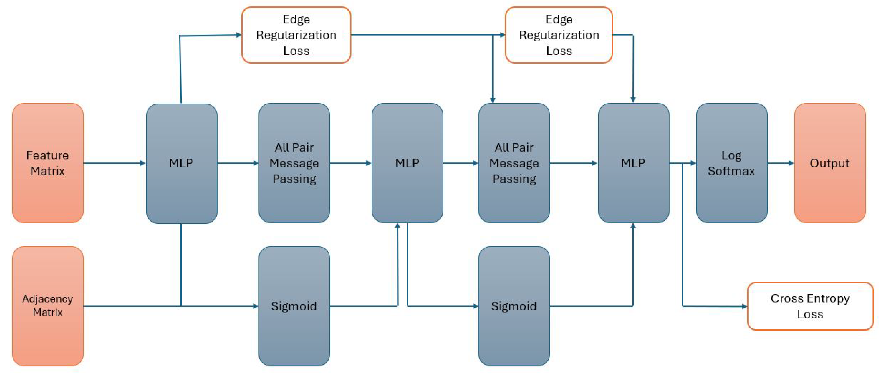
NodeFormer [20] is a graph transformer model known for its all-pair attention mechanism, enabling efficient graph data processing. Traditional graph neural networks propagate signals over a sparse adjacency matrix, while graph transformers [43] can be seen as propagating signals over a densely connected graph with layer-wise edge weights. The latter requires estimation for the N*N attention matrix and feature propagation over such a dense matrix. At each layer of the graph transformer, the embeddings of the current layer are mapped to query, key, and value vectors. Then, all pair attention is calculated for aggregating the features. Equation (4) shows how the attention operation is applied to node u:
q u ( k ) = W Q z u ( k ) , k u ( k ) = W K z u ( k ) , v ( k ) = W V z u ( k ) z u ( k + 1 ) = v = 1 N exp q u ( k ) k v ( k ) w = 1 N exp q u ( k ) k ( k ) v v ( w )
z denotes the node embeddings, and q, k, and v denote the query, key, and value vectors. The W Q , W K , and W V are learnable weights at the k-th layer. The all-pair attention operation in Equation (4) has O ( N ) complexity. However, when it gets applied to all nodes in the graph, its complexity explodes to O ( N 2 ) . To avoid this, Nodeformer decouples the summation operation from the dot product as shown in Equation (5). In this approach, the summations are independent of the node u. Therefore, the summations can be precomputed in O ( N ) complexity and then shared among all nodes. The layer embedding calculation will thus be of O ( N ) complexity:
z u ( l + 1 ) = v = 1 N ϕ q u ϕ k v w = 1 N ϕ q u ϕ k w · v v = ϕ q u v = 1 N ϕ k v · v v ϕ q u w = 1 N ϕ k w

4. Experiments

4.1. Baseline Model

To obtain a baseline performance for the dataset in each of the three cases mentioned above, we use a vanilla MLP in each case without the use of network information. We use the same training and test data and parameters for the baseline as the rest of the models.

4.2. Node Features Ablation Study

As an ablation study, the three classifiers are run featureless (without node features). This allows the evaluation of the importance of node features for the performance of our models. If the classification performance decreases when the features are removed, that would support the claim that the node features provide useful information to the models.

4.3. Model Architectures

The experiment uses three configurations for each of the four classifiers: (1) two GCN layers attached to an MLP layer, (2) two Graph Sage layers attached to an MLP layer, (3) two graph transformer layers attached to an MLP layer, and (4) three MLP layers. The models are fed the adjacency matrix, feature matrix, and labels (binary or multi-class). The adjacency matrix considers all gene interactions within the PIN dataset and gathers its location and labels through the SFari dataset. The model structure used in the (1), (2) and (3) configurations is shown in Figure 2. Model structure for configuration (4) is shown in Figure 3.
The results of the multi-class model are evaluated using specificity and sensitivity for all four classes, accuracy, and F1 Score for the test data. The test splits are 25 percent of the original dataset and split after Graph SMOTE [42] upsampling to balance the labels. The process of upsampling not only requires us to add a row to our feature matrix to account for the new nodes but also requires us to add a row and column to our adjacency matrix to account for the new node as well. The process of adding a row to the feature matrix and a column and row to the adjacency matrix is performed for each gene selected for duplication in the upsampling. The experiment is conducted using the hyperparameters listed in Table 1.

5. Results

5.1. Binary Risk Association Classification Test Results

Table 2 displays the performance metrics of the four models employed in the binary risk association classification task. GCN demonstrates exemplary performance in specificity, achieving a perfect score of 1.00, indicating its robustness in correctly identifying true negatives. However, its sensitivity is 0.69, suggesting a relatively lower capacity to detect true positives correctly. On the other hand, the Graph Sage model displays a commendable balance between specificity (0.94) and sensitivity (0.82), showcasing its ability to discern both true negatives and true positives effectively. The MLP baseline model also exhibits competitive performance, with specificity at 0.92 and sensitivity at 0.70, positioning it between the other two models regarding overall performance metrics.
Table 3 displays the performance metrics of four distinct models employed in the binary risk association classification task. Graph Sage emerges as the top performer, exhibiting the highest F1 Score of 0.87 and an accuracy of 85.80%. The graph transformer model also demonstrates competitive performance, achieving an F1 Score of 0.75 and an accuracy of 75.01%. The Featureless GCN, Graph Sage, and graph transformer model versions present lower performance metrics.
Figure 4 is the receiver operating characteristic curve that shows the optimal threshold for classification on the test dataset. The Graph Sage model is used here and in subsequent ROC curves and t-SNE plots due to its higher performance compared to the other models.
Figure 5 shows a t-SNE chart of the Graph Sage binary risk classifier. This method allows the high-dimensional data of the graph nodes (genes) to be reduced to two for visualization while preserving the data’s local structures. The t-SNE chart shows two clear clusters for the genes associated and not associated with ASD. This indicates that the two groups are distinguishable using the Graph Sage model.

5.2. Multi-Class Risk Association Test Results

Table 4 presents specificity and sensitivity metrics for four distinct association classes in the multi-class classifier, comparing the performance of GCN, Graph Sage, graph transformer, and MLP (baseline). Across association levels—‘No Association’, ‘Low Association’, ‘Moderate Association’, and ‘High Association’—GCN consistently demonstrates high specificity, particularly excelling in identifying ‘No Association’ and ‘High Association’ classes. Graph Sage performs well in various classes, showcasing balanced sensitivity, especially notable in ‘Low Association’ and ‘High Association’. Graph transformer and MLP display lower performance.
As seen in Table 5, Graph Sage is the best performer in our test. Graph Sage obtains the highest F1 Score of 0.83 and an accuracy of 81.68%. Graph transformer achieves the second highest performance. GCN fails to achieve the performance of the baseline MLP model. The Featureless versions of the models exhibit lower performance metrics, with the Graph Sage Featureless model obtaining an F1 Score of 0.32 and an accuracy of 43.44%, and the GCN Featureless model achieving an F1 Score of 0.27 and an accuracy of 43.24%, which is far below the baseline. Thus, the graph structure and node features seem to positively impact classifier performance.
Table 6 contains the top 10 list for each class of genes based on the highest confidence.
Figure 6 shows the receiver operating characteristic curves for each risk class. From the chart, it is evident that the area under the curve values are similarly high for each of the classes, showing that the Graph Sage multi-class model has a good classification ability across all the risk levels.
Figure 7 shows a t-SNE chart of the Graph Sage multi-class risk classifier. The t-SNE chart shows a clear separation between the high- and low-risk genes. At the same time, the moderate-risk genes are spread between the high- and low-risk genes. This agrees with the intuition that the ASD risk is a spectrum ranging from low to high. The non-associated genes are tightly clustered and separate from the other genes. This shows that the model can discern between no risk association and the other risk levels.

5.3. Syndromic Test Results

Table 7 shows that GCN exhibits perfect specificity at 1.00, denoting its capability to accurately identify true negatives while achieving a sensitivity of 0.68, indicating a lowered capacity in correctly detecting true positives. Graph Sage demonstrates high performance with specificity at 0.96 and sensitivity at 0.90, effectively showing its ability to discern both true negatives and true positives. The baseline MLP model shows comparable performance to GCN. Graph transformer displays balanced performance.
Table 8 shows that Graph Sage performs the best, exhibiting the highest F1 Score of 0.90 and an accuracy of 90.22%. The MLP model shows lower performance with an F1 Score of 0.86 and an accuracy of 86.39%. In contrast, the Featureless versions of GCN, Graph Sage, and graph transformer demonstrate much lower performance metrics, with the Graph Sage Featureless model attaining an F1 Score of 0.51 and an accuracy of 46.71%. The results are in line with what we observed from the binary risk classification.
Table 9 shows the top 10 genes for each class. These genes are ranked based on their confidence levels within their respective classes, offering insights into potential associations or relevance to syndromic and non-syndromic conditions. From the list of syndromic genes, many of them are associated with brain development or neuronal development syndromes (TRIP12 [44], NSD1 [45], CTNND2 [46], CADPS2 [47], MEF2C [48], SOX5 [49], and GRIP1 [50]). In contrast, most non-syndromic genes do not have a clear connection with the brain or neural development. This indicates that the model can differentiate between ASD-related and non-related genes.
Figure 8 shows the receiver operating characteristic curve for the syndromic classification.
Figure 9 shows that the syndromic and nonsyndromic genes form two separate clusters, thus showing the ability of the model to distinguish the two classes.

6. Discussion

The results highlight that Graph Sage surpasses the baseline model in every case. The GCN surpasses the baseline in most cases but not all. This implies that while graph structures offer valuable information for the three classification problems, their utility may differ in specific contexts. The graph transformer model does not surpass the Graph Sage model in our experiments. It remains to be seen whether a larger dataset will improve the graph transformer model performance beyond the other models. The featureless models perform significantly worse than their counterparts in every case. This shows that the node features (Chromosome band locations) also contribute heavily to the classification. From the t-SNE charts, we can see clear clusters forming for each of the classes. In the case of multi-class risk association, the moderate-risk genes seem to fall in between the high-risk and low-risk genes. This shows that the risk levels are a spectrum ranging from low to high. Analyzing the top genes shows that the ASD risk-associated genes discovered by the models tend to be genes connected to brain or neuronal development. This further shows the ability of the models to distinguish the risk levels. However, further study of the top genes is needed before we can confirm this.
Limitations of our study can stem from the source datasets. For example, autism datasets such as Sfari tend to contain data from clinical populations, and thus they could exclude individuals with mild levels of autism. Therefore, our models could also be biased towards severe autism levels. Another potential source for bias is the under-representation of certain groups such as minority groups from the datasets. This could affect the classification accuracy of models when it comes to those populations. The benefits of our approach include the ability for early identification and intervention. In the case of autism, such early interventions can improve therapy outcomes. Research has shown that involving pediatricians as initial diagnosticians in multidisciplinary evaluations for young children with ASD [51]. The biomarkers identified by our method could be used alongside other behavioral and brain imaging techniques as a comprehensive early diagnosis workflow. Since our method has good explainability through predictive features and t-SNE visualizations, it gives confidence to doctors and patients when used in a diagnostic setting.
Our method also holds promise for targeted therapeutic interventions for individuals with autism. Precision medicine approaches can be developed to target underlying genetic mechanisms contributing to ASD. This may include pharmacological interventions aimed at modulating neurotransmitter systems or gene therapy strategies to correct genetic abnormalities.

7. Conclusions

The experiment demonstrates the efficacy of graph neural networks in assessing the risk of gene association with ASD and identifying whether a gene is syndromic. Specifically, our findings highlight Graph Sage as particularly promising in uncovering correlations related to ASD. This success suggests broader applications of this model in diverse ASD-related domains, potentially including specific disorders within the autism spectrum. Moreover, the results indicate that leveraging networks can notably enhance model performance, motivating further exploration into more advanced graph neural network models. This groundwork lays a strong foundation for developing a robust tool to identify genes associated with neurological disorders.

Author Contributions

Conceptualization, D.B.; methodology, D.B., and K.R.; software, D.B. and K.R.; validation, D.B. and K.R.; resources, D.B.; writing—original draft preparation, K.R.; writing—review and editing, D.B.; supervision, D.B.; project administration, D.B.; funding acquisition, D.B. All authors have read and agreed to the published version of the manuscript.

Funding

This research was funded by Fairfield University School of Engineering and Computing faculty startup grant (D.B.).

Institutional Review Board Statement

Not applicable.

Data Availability Statement

The dataset used in this study is derived from publicly available datasets. As such, the authors will provide the code required to generate the dataset in a public repository.

Conflicts of Interest

The authors do not have any conflicts of interest to declare.

References

  1. Lord, C.; Elsabbagh, M.; Baird, G.; Veenstra-Vanderweele, J. Autism spectrum disorder. Lancet 2018, 392, 508–520. [Google Scholar] [CrossRef]
  2. Tick, B.; Bolton, P.; Happé, F.; Rutter, M.; Rijsdijk, F. Heritability of autism spectrum disorders: A meta-analysis of twin studies. J. Child Psychol. Psychiatry 2016, 57, 585–595. [Google Scholar] [CrossRef]
  3. Samocha, K.; Robinson, E.; Sanders, S.; Stevens, C.; Sabo, A.; McGrath, L.; Kosmicki, J.; Rehnström, K.; Mallick, S.; Kirby, A.; et al. A framework for the interpretation of de novo mutation in human disease. Nat. Genet. 2014, 46, 944–950. [Google Scholar] [CrossRef] [PubMed]
  4. Iossifov, I.; O’Roak, B.; Sanders, S.; Ronemus, M.; Krumm, N.; Levy, D.; Stessman, H.; Witherspoon, K.; Vives, L.; Patterson, K.; et al. The contribution of de novo coding mutations to autism spectrum disorder. Nature 2014, 515, 216–221. [Google Scholar] [CrossRef]
  5. Veltman, J.; Brunner, H. De novo mutations in human genetic disease. Nat. Rev. Genet. 2012, 13, 565–575. [Google Scholar] [CrossRef] [PubMed]
  6. Gratten, J.; Visscher, P.; Mowry, B.; Wray, N. Interpreting the role of de novo protein-coding mutations in neuropsychiatric disease. Nat. Genet. 2013, 45, 234–238. [Google Scholar] [CrossRef] [PubMed]
  7. Ramaswami, G.; Geschwind, D.H. Chapter 21—Genetics of autism spectrum disorder. In Handbook of Clinical Neurology; Geschwind, D.H., Paulson, H.L., Klein, C., Eds.; Neurogenetics, Part I; Elsevier: Amsterdam, The Netherlands, 2018; Volume 147, pp. 321–329. [Google Scholar] [CrossRef]
  8. Alarcón, M.; Abrahams, B.S.; Stone, J.L.; Duvall, J.A.; Perederiy, J.V.; Bomar, J.M.; Sebat, J.; Wigler, M.; Martin, C.L.; Ledbetter, D.H.; et al. Linkage, Association, and Gene-Expression Analyses Identify CNTNAP2 as an Autism-Susceptibility Gene. Am. J. Hum. Genet. 2008, 82, 150–159. [Google Scholar] [CrossRef]
  9. Shaikh, T. Copy Number Variation Disorders. Curr. Genet. Med. Rep. 2017, 5, 183–190. [Google Scholar] [CrossRef]
  10. Autism Spectrum Disorder Working Group of the Psychiatric Genomics Consortium; BUPGEN; Major Depressive Disorder Working Group of the Psychiatric Genomics Consortium; 23 and Me Research Team; Grove, J.; Ripke, S.; Als, T.; Mattheisen, M.; Walters, R.; Won, H.; et al. Identification of common genetic risk variants for autism spectrum disorder. Nat. Genet. 2019, 51, 431–444. [Google Scholar] [CrossRef]
  11. Bray, P.F.; Jones, C.I.; Soranzo, N.; Ouwehand, W.H. Chapter 4—Platelet Genomics. In Platelets, 3rd ed.; Michelson, A.D., Ed.; Academic Press: Cambridge, MA, USA, 2013; pp. 67–89. [Google Scholar] [CrossRef]
  12. Anney, R.; Klei, L.; Pinto, D.; Almeida, J.; Bacchelli, E.; Baird, G.; Bolshakova, N.; Bölte, S.; Bolton, P.F.; Bourgeron, T.; et al. Individual common variants exert weak effects on the risk for autism spectrum disorders. Hum. Mol. Genet. 2012, 21, 4781–4792. [Google Scholar] [CrossRef]
  13. Kolchanov, N.A.; Anan’ko, E.A.; Kolpakov, F.A.; Podkolodnaya, O.A.; Ignat’eva, E.V.; Goryachkovskaya, T.N.; Stepanenko, I.L. Gene Networks. Mol. Biol. 2000, 34, 449–460. [Google Scholar] [CrossRef]
  14. Gaugler, T.; Klei, L.; Sanders, S.; Bodea, C.; Goldberg, A.; Lee, A.; Mahajan, M.; Manaa, D.; Pawitan, Y.; Reichert, J.; et al. Most genetic risk for autism resides with common variation. Nat. Genet. 2014, 46, 881–885. [Google Scholar] [CrossRef] [PubMed]
  15. Pereanu, W.; Larsen, E.; Das, I.; Estevez, M.; Sarkar, A.; Spring-Pearson, S.; Kollu, R.; Basu, S.; Banerjee-Basu, S. AutDB: A platform to decode the genetic architecture of autism. Nucleic Acids Res. 2017, 46, D1049–D1054. [Google Scholar] [CrossRef] [PubMed]
  16. Bai, Y.; Ding, H.; Bian, S.; Chen, T.; Sun, Y.; Wang, W. Simgnn. In Proceedings of the Twelfth ACM International Conference on Web Search and Data Mining, Melbourne, VIC, Australia, 11–15 February 2019. [Google Scholar] [CrossRef]
  17. Kim, C.; Haeseong, M.; Hwang, H.J. Near: Neighborhood edge aggregator for graph classification. arXiv 2019, arXiv:1909.02746. [Google Scholar] [CrossRef]
  18. Tran, D.V.; Navarin, N.; Sperduti, A. On filter size in graph convolutional networks. In Proceedings of the 2018 IEEE Symposium Series on Computational Intelligence (SSCI), Bangalore, India, 18–21 November 2018. [Google Scholar] [CrossRef]
  19. Riccardi, K.; Bandara, D. Autism Risk Classification using Graph Neural Networks Applied to Gene Interaction Data. In Proceedings of the 2023 International Conference on Computational Science and Computational Intelligence (CSCI), Las Vegas, NV, USA, 13–15 December 2023. in press. [Google Scholar]
  20. Wu, Q.; Zhao, W.; Li, Z.; Wipf, D.P.; Yan, J. Nodeformer: A scalable graph structure learning transformer for node classification. Adv. Neural Inf. Process. Syst. 2022, 35, 27387–27401. [Google Scholar]
  21. Hamilton, W.; Ying, R.; Leskovec, J. Inductive Representation Learning on Large Graphs. In Advances in Neural Information Processing Systems; NeurIPS Foundation: San Diego, CA, USA, 2017. [Google Scholar]
  22. Kipf, T.N.; Welling, M. Semi-Supervised Classification with Graph Convolutional Networks. In Proceedings of the International Conference on Learning Representations, Toulon, France, 24–26 April 2017. [Google Scholar]
  23. Bralten, J.; van Hulzen, K.J.; Martens, M.B.; Galesloot, T.E.; Arias Vasquez, A.; Kiemeney, L.A.; Buitelaar, J.K.; Muntjewerff, J.W.; Franke, B.; Poelmans, G. Autism spectrum disorders and autistic traits share genetics and biology. Mol. Psychiatry 2018, 23, 1205–1212. [Google Scholar] [CrossRef]
  24. Grove, J.; Ripke, S.; Als, T.D.; Mattheisen, M.; Walters, R.K.; Won, H.; Pallesen, J.; Agerbo, E.; Andreassen, O.A.; Anney, R.; et al. Identification of common genetic risk variants for autism spectrum disorder. Nat. Genet. 2019, 51, 431–444. [Google Scholar] [CrossRef] [PubMed]
  25. Krishnan, A.; Zhang, R.; Yao, V.; Theesfeld, C.L.; Wong, A.K.; Tadych, A.; Volfovsky, N.; Packer, A.; Lash, A.E.; Troyanskaya, O.G. Genome-wide prediction and functional characterization of the genetic basis of autism spectrum disorder. Nat. Neurosci. 2016, 19, 1454–1462. [Google Scholar] [CrossRef] [PubMed]
  26. Rahman, M.M.; Usman, O.L.; Muniyandi, R.C.; Sahran, S.; Mohamed, S.; Razak, R.A. A review of machine learning methods of feature selection and classification for autism spectrum disorder. Brain Sci. 2020, 10, 949. [Google Scholar] [CrossRef]
  27. Ismail, E.A.R.; Gad, W.; Hashem, M. Hec-asd: A hybrid ensemble-based classification model for predicting autism spectrum disorder disease genes. BMC Bioinform. 2022, 23, 554. [Google Scholar] [CrossRef]
  28. Lin, Y.; Rajadhyaksha, A.M.; Potash, J.B.; Han, S. A machine learning approach to predicting autism risk genes: Validation of known genes and discovery of new candidates. bioRxiv 2018. [Google Scholar] [CrossRef]
  29. Brueggeman, L.; Koomar, T.; Michaelson, J.J. Forecasting autism gene discovery with machine learning and genome-scale data. bioRxiv 2018. [Google Scholar] [CrossRef]
  30. Gandhi, T.; Zhong, J.; Mathivanan, S.; Karthick, L.; Chandrika, K.; Mohan, S.S.; Sharma, S.; Pinkert, S.; Nagaraju, S.; Periaswamy, B.; et al. Analysis of the human protein interactome and comparison with yeast, worm and fly interaction datasets. Nat. Genet. 2006, 38, 285–293. [Google Scholar] [CrossRef] [PubMed]
  31. Krumm, N.; O’Roak, B.J.; Shendure, J.; Eichler, E.E. A de novo convergence of autism genetics and molecular neuroscience. Trends Neurosci. 2014, 37, 95–105. [Google Scholar] [CrossRef] [PubMed]
  32. Hormozdiari, F.; Penn, O.; Borenstein, E.; Eichler, E.E. The discovery of integrated gene networks for autism and related disorders. Genome Res. 2015, 25, 142–154. [Google Scholar] [CrossRef]
  33. Liu, L.; Lei, J.; Roeder, K. Network assisted analysis to reveal the genetic basis of autism. Ann. Appl. Stat. 2015, 9, 1571. [Google Scholar] [CrossRef]
  34. Feng, J.; Zeng, A.; Chen, Y.; Payne, P.; Li, F. Signaling interaction link prediction using deep graph neural networks integrating protein-protein interactions and omics data. bioRxiv 2020. [Google Scholar] [CrossRef]
  35. Wang, Z.; Xu, Y.; Peng, D.; Gao, J.; Lu, F. Brain functional activity-based classification of autism spectrum disorder using an attention-based graph neural network combined with gene expression. Cereb. Cortex 2022, 33, 6407–6419. [Google Scholar] [CrossRef]
  36. Beyreli, I.; Karakahya, O.; Cicek, A.E. DeepND: Deep multitask learning of gene risk for comorbid neurodevelopmental disorders. Patterns 2022, 3, 100524. [Google Scholar] [CrossRef]
  37. Lu, H. and Uddin, S. A weighted patient network-based framework for predicting chronic diseases using graph neural networks. Sci. Rep. 2021, 11, 22607. [Google Scholar] [CrossRef]
  38. Wang, H.; Avillach, P. Genotype-Based Deep Learning in Autism Spectrum Disorder: Diagnostic Classification and Prognostic Prediction Using Common Genetic Variants. JMIR Med. Inform. 2021, 9, e24754. [Google Scholar] [CrossRef] [PubMed]
  39. Motsinger, A.A.; Lee, S.L.; Mellick, G.; Ritchie, M.D. GPNN: Power studies and applications of a neural network method for detecting gene-gene interactions in studies of human disease. BMC Bioinform. 2006, 7, 39. [Google Scholar] [CrossRef] [PubMed]
  40. Laksshman, S.; Bhat, R.; Viswanath, V.; Li, X. DeepBipolar: Identifying genomic mutations for bipolar disorder via deep learning. Hum. Mutat. 2017, 38, 1217–1224. [Google Scholar] [CrossRef] [PubMed]
  41. Abrahams, B.; Arking, D.; Campbell, D.; Mefford, H.; Morrow, E.; Weiss, L.; Menashe, I.; Wadkins, T.; Banerjee-Basu, S.; Packer, A. SFARI Gene 2.0: A community-driven knowledgebase for the autism spectrum disorders (ASDs). Mol. Autism 2013, 4, 36. [Google Scholar] [CrossRef]
  42. Zhao, T.; Zhang, X.; Wang, S. Graphsmote: Imbalanced node classification on graphs with graph neural networks. In Proceedings of the 14th ACM International Conference on Web Search and Data Mining, Jerusalem, Israel, 8–12 March 2021; pp. 833–841. [Google Scholar]
  43. Wang, H.; Guo, F.; Du, M.; Wang, G.; Cao, C. A novel method for drug-target interaction prediction based on graph transformers model. BMC Bioinform. 2022, 23, 459. [Google Scholar] [CrossRef] [PubMed]
  44. Donoghue, T.; Garrity, L.; Ziolkowski, A.; McPhillips, M.; Buckman, M.; Goel, H. Novel de novo trip12 mutation reveals variable phenotypic presentation while emphasizing core features of trip12 variations. Am. J. Med. Genet. Part A 2020, 182, 1801–1806. [Google Scholar] [CrossRef] [PubMed]
  45. Baujat, G.; Rio, M.; Rossignol, S.; Sanlaville, D.; Lyonnet, S.; Merrer, M.L.; Münnich, A.; Gicquel, C.; Cormier-Daire, V.; Colleaux, L. Paradoxical nsd1 mutations in beckwith-wiedemann syndrome and 11p15 anomalies in sotos syndrome. Am. J. Hum. Genet. 2004, 74, 715–720. [Google Scholar] [CrossRef] [PubMed]
  46. Nakagawa, N.; Li, J.; Yabuno-Nakagawa, K.; Eom, T.Y.; Cowles, M.W.; Mapp, T.; Taylor, R.; Anton, E.S. Apc sets the wnt tone necessary for cerebral cortical progenitor development. Genes Dev. 2017, 31, 1679–1692. [Google Scholar] [CrossRef] [PubMed]
  47. Sadakata, T.; Furuichi, T. Developmentally regulated Ca2+-dependent activator protein for secretion 2 (caps2) is involved in bdnf secretion and is associated with autism susceptibility. Cerebellum 2009, 8, 312–322. [Google Scholar] [CrossRef]
  48. Chaudhary, R.; Agarwal, V.; Kaushik, A.S.; Rehman, M. Involvement of myocyte enhancer factor 2c in the pathogenesis of autism spectrum disorder. Heliyon 2021, 7, e06854. [Google Scholar] [CrossRef]
  49. Kanlayaprasit, S.; Thongkorn, S.; Panjabud, P.; Jindatip, D.; Hu, V.W.; Kikkawa, T.; Osumi, N.; Sarachana, T. Autism-related transcription factors underlying the sex-specific effects of prenatal bisphenol a exposure on transcriptome-interactome profiles in the offspring prefrontal cortex. Int. J. Mol. Sci. 2021, 22, 13201. [Google Scholar] [CrossRef] [PubMed]
  50. Tan, H.L.; Chiu, S.L.; Zhu, Q.; Huganir, R.L. Grip1 regulates synaptic plasticity and learning and memory. Proc. Natl. Acad. Sci. USA 2020, 117, 25085–25091. [Google Scholar] [CrossRef] [PubMed]
  51. Ahlers, K.; Gabrielsen, T.P.; Ellzey, A.; Brady, A.M.; Litchford, A.; Fox, J.; Nguyen, Q.; Carbone, P.S. A pilot project using pediatricians as initial diagnosticians in multidisciplinary autism evaluations for young children. J. Dev. Behav. Pediatr. 2019, 40, 1–11. [Google Scholar] [CrossRef] [PubMed]
Figure 1. (A) Sfari dataset format, (B) PIN dataset format, (C) nodes, node features, and node labels generated using Sfari dataset, (D) adjacency matrix created using PIN dataset.
Genes 15 00447 g001
Figure 2. Model structure of the MLP, GCN, and Graph Sage models.
Genes 15 00447 g002
Figure 3. Model structure of the graph transformer model.
Genes 15 00447 g003
Figure 4. The receiver operating characteristic curve for the binary risk association classification using the Graph Sage model.
Genes 15 00447 g004
Figure 5. Visualization of the Graph Sage model genes using t-distributed stochastic neighbor embedding (t-SNE). Different colors represent different classes.
Genes 15 00447 g005
Figure 6. The ROC curve for multi-class risk association classification.
Genes 15 00447 g006
Figure 7. Visualization of the Graph Sage multi-class classifier genes using t-distributed stochastic neighbor embedding (t-SNE). Different colors represent different classes.
Genes 15 00447 g007
Figure 8. The receiver operating characteristic curve for syndromic classification.
Genes 15 00447 g008
Figure 9. Visualization of the Graph Sage syndromic classifier genes using t-distributed stochastic neighbor embedding (t-SNE). Different colors represent different classes.
Genes 15 00447 g009
Table 1. Parameters used for training the models.
Parameter NameValue
Learning rate0.001
Weight decay 5 × 10 4
epsilon 1 × 10 4
Batch size64
Epoch5000
Output FunctionLog Softmax
Activation FunctionreLu
OptimizerAdamW
Table 2. The performance of the four models in the binary risk association classification.
Model NameSpecificitySensitivity
MLP0.920.70
GCN1.000.69
Graph Sage0.940.82
Graph T/F0.760.74
Table 3. The F1 Score and accuracy for all five binary graph neural network models.
Model NameF1 ScoreAccuracy
GCN0.7377.08
Graph Sage0.8785.80
Graph T/F0.7575.01
MLP0.7878.88
GCN Featureless0.7263.57
Graph Sage Featureless0.4166.61
Graph T/F Featureless0.2946.36
Table 4. The specificity and sensitivity for all four classes in the multi-class graph neural network model.
Class NumberGCNGraph SageGraph TransformerMLP
No Association1.00/0.940.95/0.800.83/0.780.96/0.76
Low Association1.00/0.760.94/1.000.95/0.880.90/0.89
Moderate Association1.00/0.610.98/0.800.96/0.730.97/0.65
High Association1.00/0.990.98/0.890.97/0.900.97/0.75
Table 5. The F1 Score and accuracy for all five multi-class graph neural network models.
Model NameF1 ScoreAccuracy
MLP0.7269.80
GCN0.5655.19
Graph Sage0.8381.68
Graph T/F0.7978.13
GCN Featureless0.2743.24
Graph Sage Featureless0.3243.44
Graph T/F Featureless0.2026.01
Table 6. The highest confidence level genes as predicted by the Graph Sage multi-class model for the various risk levels.
High AssociationModerate AssociationLow Association
FMRTOP3BPPP3CA
TCFELAVL2TCEAL1
HRAHTR3CHCN1
CULKHDRBS2IKZF1
PTERBFOX1BAIAP2L1
CHDCTNND2TRPC5
NLGNPON1YWHAZ
CTNNBPCDH10CACNB1
KMT2PLNCACNB3
NSDCNTNAP4PC
Table 7. The specificity and sensitivity for all four of our models in the syndromic classification.
Model NameSpecificitySensitivity
MLP0.970.75
GCN1.000.68
Graph Sage0.960.90
Graph T/F0.930.82
Table 8. The F1 Score and accuracy for all five syndromic classifiers.
Model NameF1 ScoreAccuracy
MLP0.8686.39
GCN0.7878.66
Graph Sage0.9090.22
Graph T/F0.7876.46
GCN Featureless0.7248.16
Graph Sage Featureless0.5146.71
Graph T/F Featureless0.2943.04
Table 9. The top 10 genes based on confidence for both syndromic and non-syndromic classes.
Non-SyndromicSyndromic
CDK11BTRIP12
CCL21TNRC6B
MATR3NSD1
DCXCTNND2
ATXN1CADPS2
HOXB13MST1R
MIR101-1TSPAN7
WNT1MEF2C
C4ORF6SOX5
CCDC27GRIP1
Disclaimer/Publisher’s Note: The statements, opinions and data contained in all publications are solely those of the individual author(s) and contributor(s) and not of MDPI and/or the editor(s). MDPI and/or the editor(s) disclaim responsibility for any injury to people or property resulting from any ideas, methods, instructions or products referred to in the content.

