Efficient Selection of Gaussian Kernel SVM Parameters for Imbalanced Data
Abstract
1. Introduction
- The hyperplane used in the SVM algorithm will skew toward the minority class if the training dataset is imbalanced. The objective of the conventional SVM is to maximize the overall accuracy and an equal misclassification cost is assumed in the classifiers.
- The performance of the SVM highly depends on the parameter selection and its kernel selection. In general, it can be very time consuming to optimize its parameters by using a grid search.
2. Materials and Methods
2.1. b-SVM
2.2. Min-Max Gamma Selection
| Algorithm 1: Min-max gamma selection |
 |
2.3. Performance Measures
2.4. Simulation Study
2.5. Real Datasets
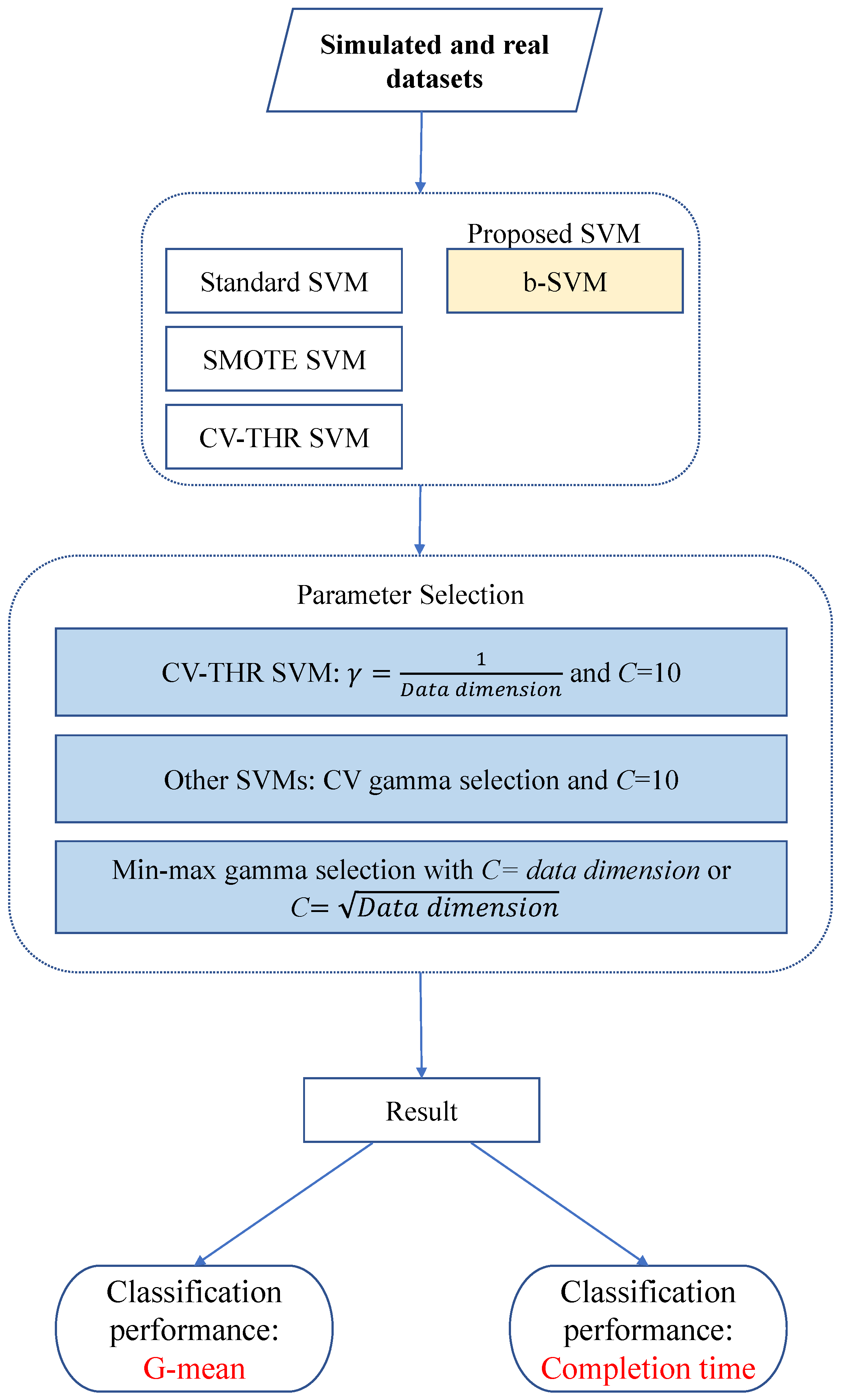
2.6. Flow Chart for Experiments
3. Results
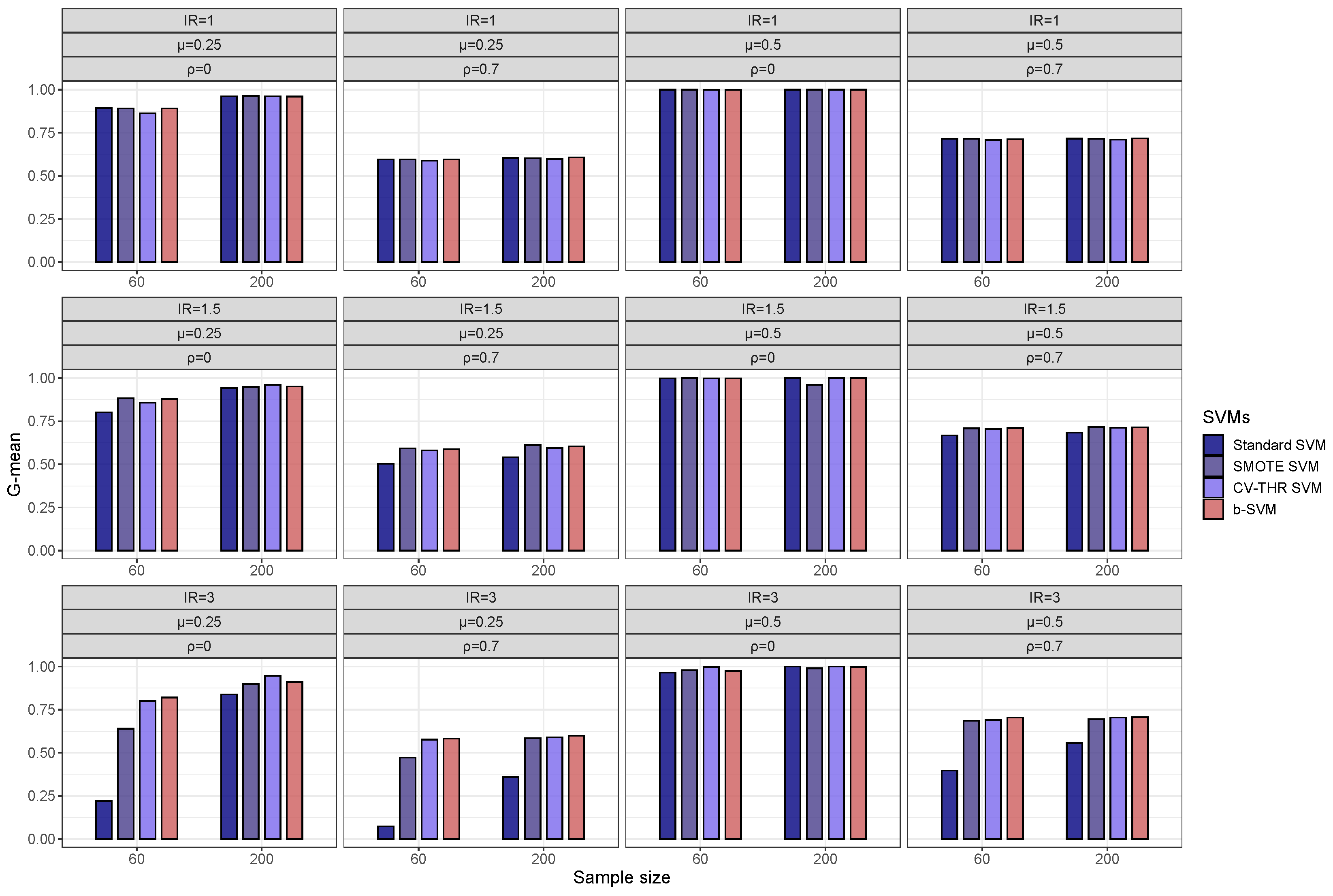
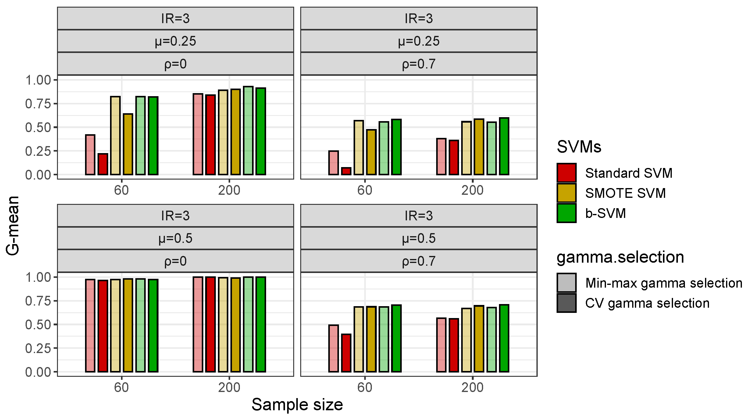
3.1. Simulation Study
3.2. Real Datasets
4. Conclusions
Author Contributions
Funding
Institutional Review Board Statement
Informed Consent Statement
Data Availability Statement
Acknowledgments
Conflicts of Interest
References
- Ding, S.; Chen, L. Intelligent Optimization Methods for High-Dimensional Data Classification for Support Vector Machine. Intell. Inf. Manag. 2010, 2, 2017. [Google Scholar] [CrossRef]
- Kubat, M.; Matwin, S. Addressing the Curse of Imbalanced Training Sets: One-Sided Selection. Int. Conf. Mach. Learn. 1997, 97, 179–186. [Google Scholar]
- Chawla, N.; Bowyer, K.; Hall, L.; Kegelmeyer, W. SMOTE: Synthetic minority over-sampling technique. J. Artif. Intell. Res. 2002, 16, 321–357. [Google Scholar] [CrossRef]
- Han, H.; Wang, W.; Mao, B. Borderline-SMOTE: A New Over-Sampling Method in imbalanced data sets learning. In Proceedings of the International Conference on Intelligent Computing, ICIC 2005, Hefei, China, 23–26 August 2005; pp. 878–887. [Google Scholar]
- Veropoulos, K.; Campbell, C.; Cristianini, N. Controlling the sensitivity of support vector machines. Int. Jt. Conf. Artif. Intell. 1999, 99, 55–60. [Google Scholar]
- Akbani, R.; Kwek, S.; Japkowicz, N. Applying Support Vector Machines to Imbalanced Datasets. Eur. Conf. Mach. Learn. 2004, 3201, 39–50. [Google Scholar]
- Cao, P.; Zhao, D.; Zaiane, O. An optimized cost-sensitive SVM forimbalanced data learning. In Proceedings of the 17th Pacific-Asia Conference, PAKDD 2013, Gold Coast, Australia, 14–17 April 2013; Volume 7819, pp. 280–292. [Google Scholar]
- Duan, W.; Jing, L.; Lu, X. Imbalanced data classification using cost-sensitive support vector machine based on information entropy. Adv. Mat. Res. 2014, 989–994, 1756–1761. [Google Scholar] [CrossRef]
- Wu, G.; Chang, E. KBA: Kernel boundary alignment considering imbalanced data distribution. IEEE Trans. Knowl. Data Eng. 2005, 17, 786–795. [Google Scholar] [CrossRef]
- Lin, W.; Chen, J. Class-imbalanced classifiers for high-dimensional data. Brief. Bioinform. 2012, 14, 13–26. [Google Scholar] [CrossRef] [PubMed]
- Nùñez, H.; Gonzalez-Abril, L.; Angulo, C. A post-processing strategy for SVM learning from unbalanced data. In Proceedings of the 19th European Symposium on Artificial Neural Networks, Computational Intelligence and Machine Learning, Bruges, Belgium, 27–29 April 2011; pp. 195–200. [Google Scholar]
- Yu, H.; Mu, C.; Sun, C.; Yang, W.; Yang, X.; Zuo, X. Support vector machine-based optimized decision threshold adjustment strategy for classifying imbalanced data. Knowl. Based Syst. 2015, 76, 67–78. [Google Scholar] [CrossRef]
- Brank, J.; Grobelnik, M.; Milić-Frayling, N.; Mladenić, D. Training Text Classifiers with SVM on Very Few Positive Examples; Technical Report MSR-TR-2003-34; Microsoft Research: Redmond, WA, USA, 2003. [Google Scholar]
- Shunjie, H.; Qubo, C.; Meng, H. Parameter selection in SVM with RBF kernel function. J. Zhe Jiang Univ. Technol. 2007, 35, 163–167. [Google Scholar]
- Syarif, I.; Prugel-Bennett, A.; Wills, G. SVM parameter optimization using grid search and genetic algorithm to improve classification performance. TELKOMNIKA 2016, 14, 1502–1509. [Google Scholar] [CrossRef]
- Huang, C.; Dun, D. A distributed PSO–SVM hybrid system with feature selection and parameter optimization. Appl. Soft Comput. 2008, 8, 1381–1391. [Google Scholar] [CrossRef]
- Lin, S.; Ying, K.; Chen, S.; Lee, Z. Particle swarm optimization for parameter determination and feature selection of support vector machines. Expert Syst. Appl. 2008, 35, 1817–1824. [Google Scholar] [CrossRef]
- Ren, Y.; Bai, G. Determination of optimal SVM parameters by using GA/PSO. J. Comput. 2008, 5, 1160–1168. [Google Scholar] [CrossRef]
- Chapelle, O.; Vapnik, V.; Bousquet, O.; Mukherjee, S. Choosing multiple parameters for support vector machines. Mach. Learn. 2002, 46, 131–159. [Google Scholar] [CrossRef]
- Staelin, C. Parameter Selection for Support Vector Machines; Hewlett-Packard Company: Singapore, 2003. [Google Scholar]
- Fröhlich, H.; Zell, A. Efficient parameter selection for support vector machines in classification and regression via model-based global optimization. In Proceedings of the IEEE International Joint Conference on Neural Networks, 1 July–4 August 2005; Volume 3, pp. 1431–1436. [Google Scholar]
- Lichman, M. UCI Machine Learning Repository. 2013. Available online: http://archive.ics.uci.edu/ml (accessed on 12 December 2022).
- Alon, U.; Barkai, N.; Notterman, D.; Gish, K.; Ybarra, S.; Mack, D.; Levine, A. Broad patterns of gene expression revealed by clustering analysis of tumor and normal colon tissues probed by oligonucleotide arrays. Proc. Natl. Acad. Sci. USA 1999, 96, 6745–6750. [Google Scholar] [CrossRef] [PubMed]
- Nutt, C.; Mani, D.; Betensky, R.; Tamayo, P.; Cairncross, J.; Ladd, C.; Pohl, U.; Hartmann, C.; McLaughlin, M.; Batchelor, T.; et al. Gene Expression-based Classification of Malignant Gliomas Correlates Better with Survival than Histological Classification. Cancer Res. 2003, 63, 1602–1607. [Google Scholar] [PubMed]
- Yang, K.; Cai, Z.; Li, J.; Lin, G. A stable gene selection in microarray data analysis. BMC Bioinform. 2006, 7, 228. [Google Scholar] [CrossRef] [PubMed]
- Hippo, Y.; Taniguchi, H.; Tsutsumi, S.; Machida, N.; Chong, J.; Fukayama, M.; Kodama, T.; Aburatani, H. Global Gene Expression Analysis of Gastric Cancer by Oligonucleotide Microarrays. Cancer Res. 2002, 62, 233–240. [Google Scholar] [PubMed]


| Dataset | Features | / | Source |
|---|---|---|---|
| Haberman | 3 | 81/225 | [22] |
| Liver | 5 | 105/240 | [22] |
| Colon cancer | 2000 | 22/40 | [10,23] |
| Glioma2 | 4434 | 7/43 | [24,25] |
| Glioma | 4434 | 14/36 | [24,25] |
| Gastric tumor | 4522 | 8/22 | [26] |
| SVMs | L.Datasets 1 | H.Datasets 2 |
|---|---|---|
| Standard SVM | 474.14 | 887.09 |
| SMOTE SVM | 976.12 | 3277.14 |
| CV-THR SVM | 452.41 | 1011.20 |
| b-SVM | 474.85 | 902.50 |
| SVMs | Min-Max | CV |
|---|---|---|
| Standard SVM | 127.47 | 474.14 |
| SMOTE SVM | 227.30 | 976.12 |
| b-SVM | 127.43 | 474.85 |
| SVMs | Min-Max | CV |
|---|---|---|
| Standard SVM | 258.92 | 887.09 |
| SMOTE SVM | 470.05 | 3277.14 |
| b-SVM | 257.05 | 902.50 |
| SVM | |||||
|---|---|---|---|---|---|
| Dataset | Metrics | Standard | SMOTE | CV-THR | b |
| Haberman | Accuracy | 0.7213 | 0.6896 | 0.6423 | 0.7182 |
| (0.0020) | (0.0026) | (0.0045) | (0.0020) | ||
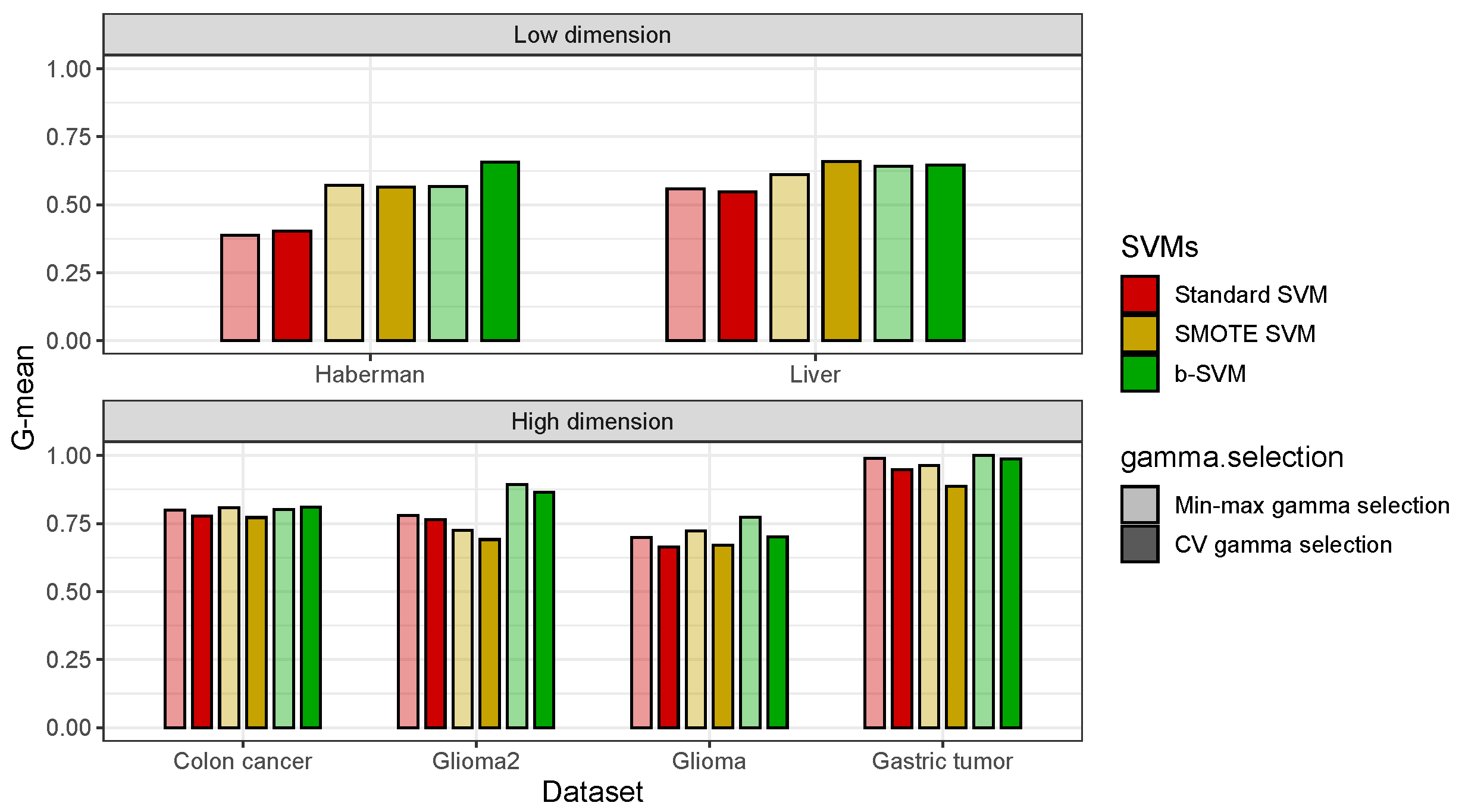
| G-mean | 0.3590 | 0.5393 | 0.5754 | 0.5974 | |
| (0.0078) | (0.0056) | (0.0046) | (0.0056) | ||
| Time (s) | 17.18 | 22.84 | 5130.64 | 16.88 | |
| Liver | Accuracy | 0.7489 | 0.6880 | 0.6879 | 0.7248 |
| (0.0015) | (0.0022) | (0.0030) | (0.0020) | ||
| G-mean | 0.5655 | 0.6152 | 0.6381 | 0.6298 | |
| (0.0043) | (0.0034) | (0.0029) | (0.0031) | ||
| Time (s) | 19.55 | 31.58 | 6641.39 | 20.66 | |
| Colon cancer | Accuracy | 0.8324 | 0.8403 | 0.8278 | 0.8307 |
| (0.0042) | (0.0037) | (0.0045) | (0.0038) | ||
| G-mean | 0.7797 | 0.7892 | 0.7949 | 0.8098 | |
| (0.0092) | (0.0095) | (0.0115) | (0.0094) | ||
| Time (s) | 7.28 | 35.81 | 2997.96 | 6.73 | |
| Glioma2 | Accuracy | 0.9340 | 0.8133 | 0.8480 | 0.8540 |
| (0.0017) | (0.0096) | (0.0054) | (0.0045) | ||
| G-mean | 0.7874 | 0.6933 | 0.8236 | 0.8650 | |
| (0.0093) | (0.0106) | (0.0116) | (0.0080) | ||
| Time (s) | 8.15 | 71.50 | 3330.43 | 7.89 | |
| Glioma | Accuracy | 0.8587 | 0.8593 | 0.7940 | 0.8587 |
| (0.0027) | (0.0030) | (0.0084) | (0.0048) | ||
| G-mean | 0.6773 | 0.6797 | 0.6963 | 0.6825 | |
| (0.0163) | (0.0165) | (0.0148) | (0.0163) | ||
| Time (s) | 7.90 | 71.56 | 3335.27 | 7.82 | |
| Gastric tumor | Accuracy | 0.9011 | 0.8889 | 0.9456 | 0.9600 |
| (0.0049) | (0.0068) | (0.0040) | (0.0030) | ||
| G-mean | 0.8310 | 0.8132 | 0.9474 | 0.9647 | |
| (0.0114) | (0.0125) | (0.0058) | (0.0053) | ||
| Time (s) | 7.60 | 66.89 | 3537.62 | 7.53 | |
Disclaimer/Publisher’s Note: The statements, opinions and data contained in all publications are solely those of the individual author(s) and contributor(s) and not of MDPI and/or the editor(s). MDPI and/or the editor(s) disclaim responsibility for any injury to people or property resulting from any ideas, methods, instructions or products referred to in the content. |
© 2023 by the authors. Licensee MDPI, Basel, Switzerland. This article is an open access article distributed under the terms and conditions of the Creative Commons Attribution (CC BY) license (https://creativecommons.org/licenses/by/4.0/).
Share and Cite
Tsai, C.-A.; Chang, Y.-J. Efficient Selection of Gaussian Kernel SVM Parameters for Imbalanced Data. Genes 2023, 14, 583. https://doi.org/10.3390/genes14030583
Tsai C-A, Chang Y-J. Efficient Selection of Gaussian Kernel SVM Parameters for Imbalanced Data. Genes. 2023; 14(3):583. https://doi.org/10.3390/genes14030583
Chicago/Turabian StyleTsai, Chen-An, and Yu-Jing Chang. 2023. "Efficient Selection of Gaussian Kernel SVM Parameters for Imbalanced Data" Genes 14, no. 3: 583. https://doi.org/10.3390/genes14030583
APA StyleTsai, C.-A., & Chang, Y.-J. (2023). Efficient Selection of Gaussian Kernel SVM Parameters for Imbalanced Data. Genes, 14(3), 583. https://doi.org/10.3390/genes14030583


