
Robust Differential Abundance Analysis of Microbiome Sequencing Data


Abstract
:1. Introduction
- 1.
- This study conducted comprehensive simulations to investigate the impact of outliers and different types of heavy-tailedness on the various DAA methods.
- 2.
- This study introduced a general M-estimation framework for DAA, which includes several methods that are robust to outliers and heavy-tailedness.
- 3.
- This study conducted extensive simulations to examine the performance of various DAA methods to address outliers and heavy-tailedness, including multiple levels of the winsorization technique and different M-estimation-based methods. The experiments demonstrated that the proposed Huber regression method based on the M-estimation framework is more stable for outliers and heavy-tailedness.
2. Materials and Methods
2.1. A Regression-Based Framework for Differential Analysis
2.1.1. CLR-Based Log-Linear Models
2.1.2. M-Estimation Framework for Differential Analysis
- 1.
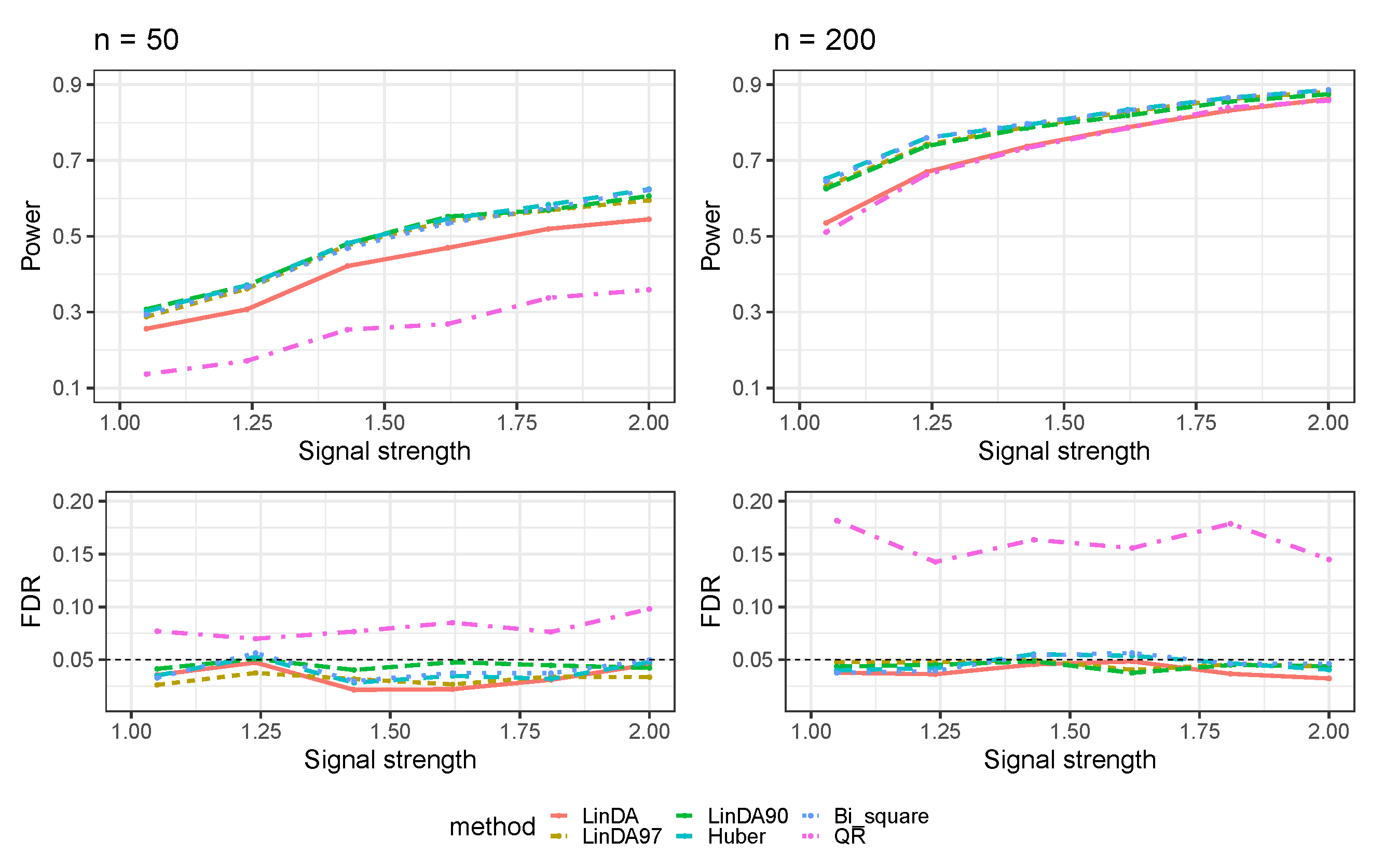
- Huber’s loss is defined aswhere c is the hyperparameter and the default value is 1.345, which is widely used in robust regression studies. Notice that the Huber estimator down-weights the influence of observations with large residuals, resulting in less impact on the estimated regression coefficients. Additionally, Huber [22] argued that if the true distribution was normal, this loss function is asymptotically 95% as efficient as least squares.
- 2.
- Tukey’s bisquare loss is defined aswhere is the standard constant for this loss function. It is worth noting that this function has been shown to possess an asymptotic efficiency of 95% with respect to linear regression for the normal distribution.
- 3.
- Quantile regression loss is defined aswhere τ represents the quantile level of interest. Notably, when , the loss function is equivalent to the loss, expressed as . The loss corresponds to the loss function utilized in the least absolute deviations (LAD) regression method.
- 1.
- For each taxon, solve the optimization problem defined in (4) to obtain the estimator and its variance estimator .
- 2.
- Calculate the mode based on , and perform mode correction to obtain the bias-corrected estimator .
- 3.
- Compute the test statistics and the p-value for each taxon.
- 4.
- Apply the BH procedure to adjust the p-values.
2.2. Winsorization
3. Results
3.1. Simulations Based on Log-Linear Models
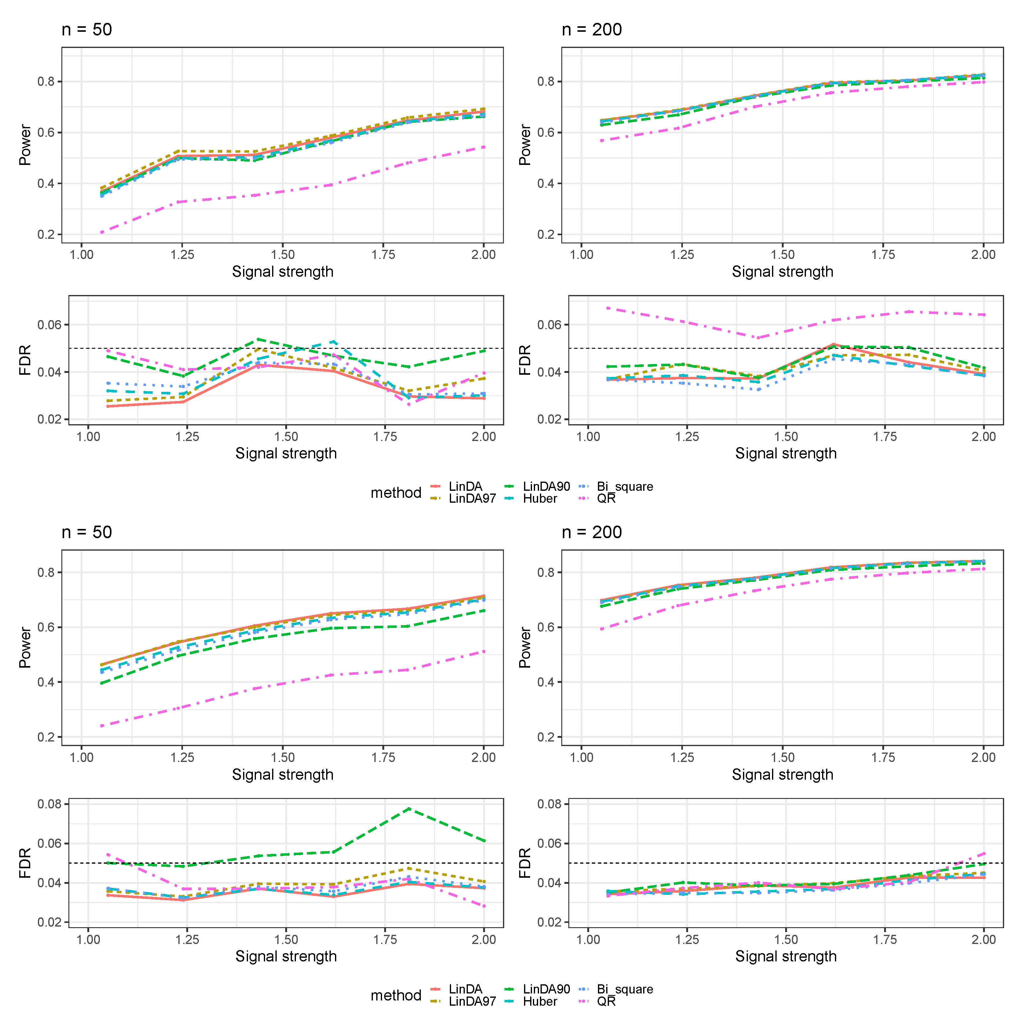
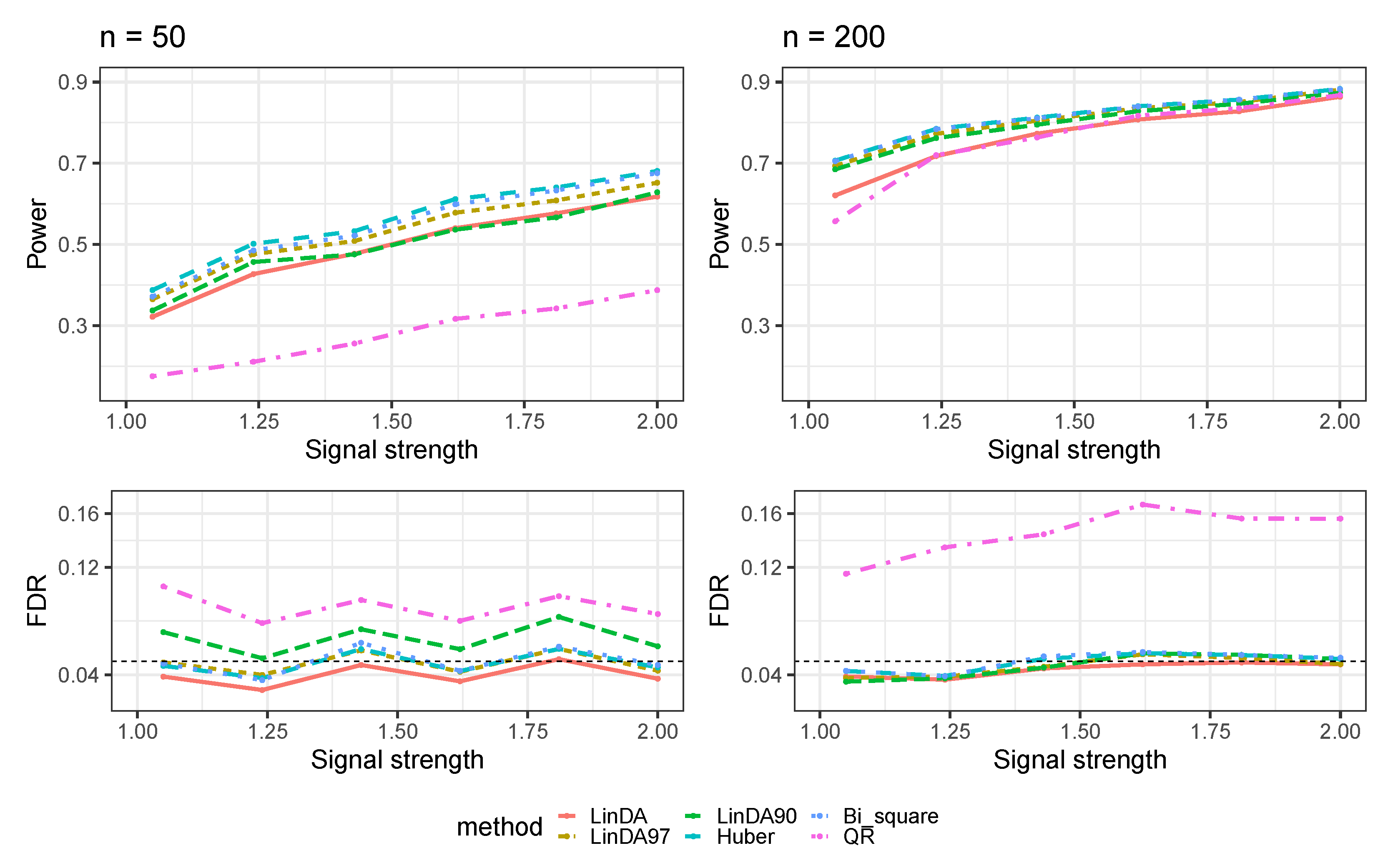
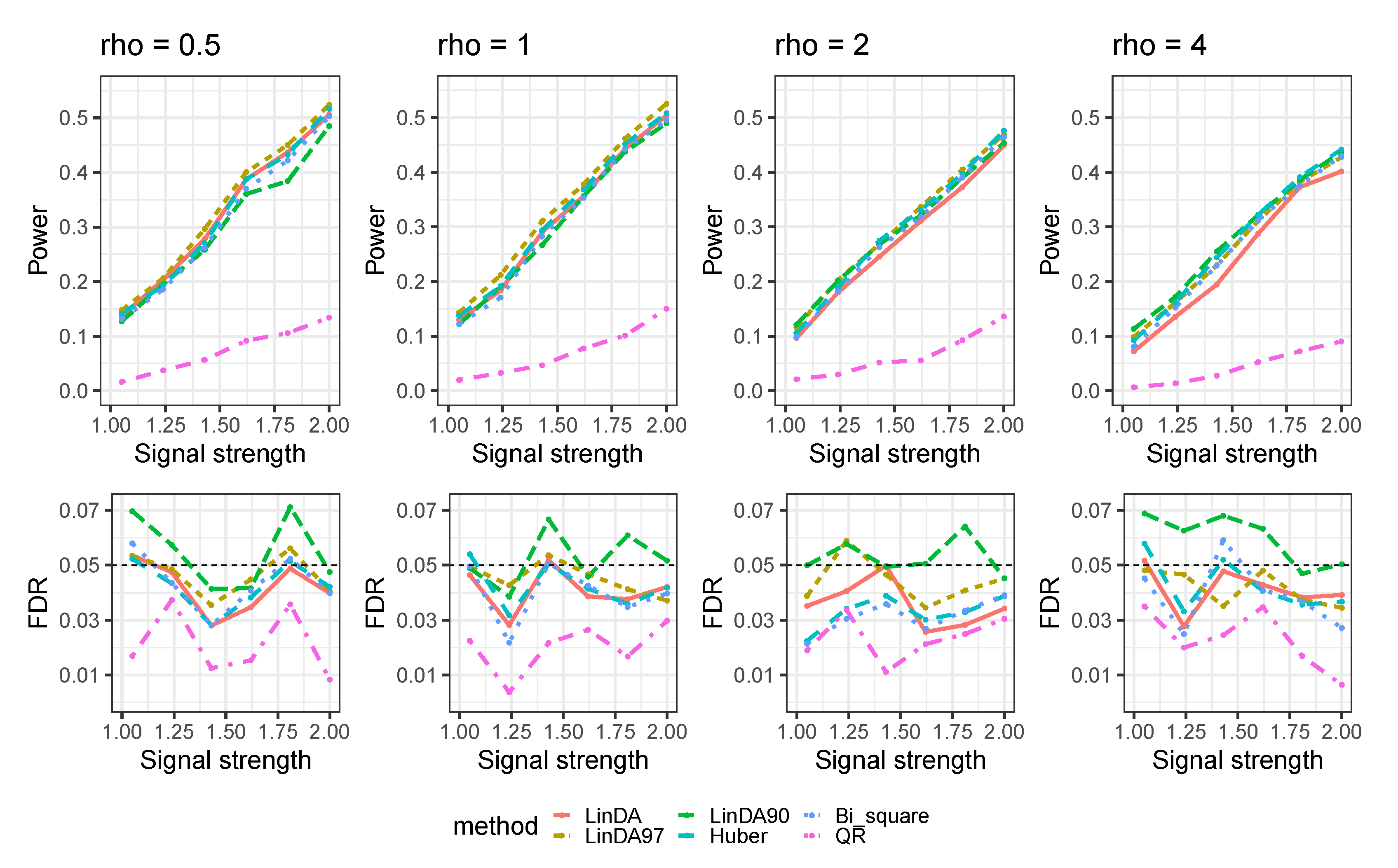
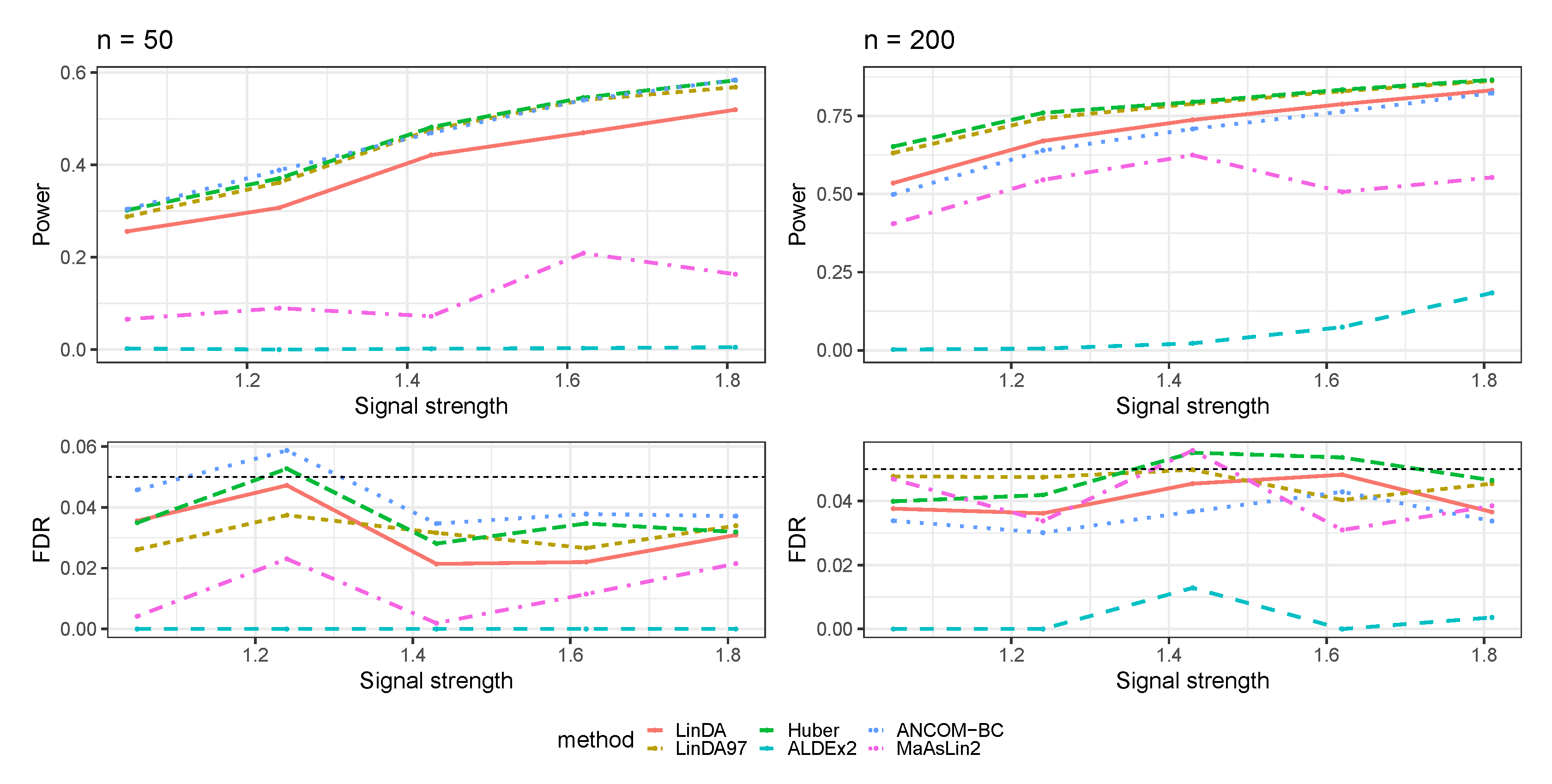
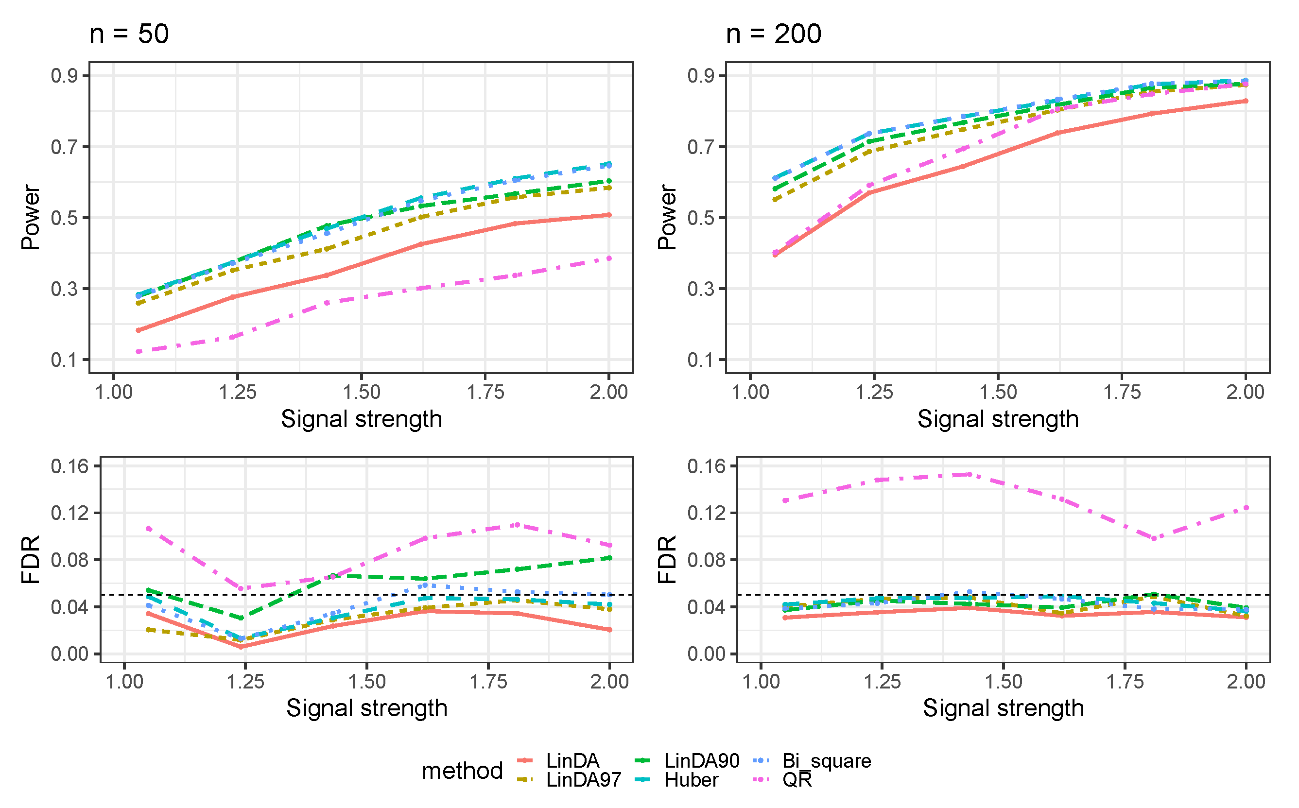
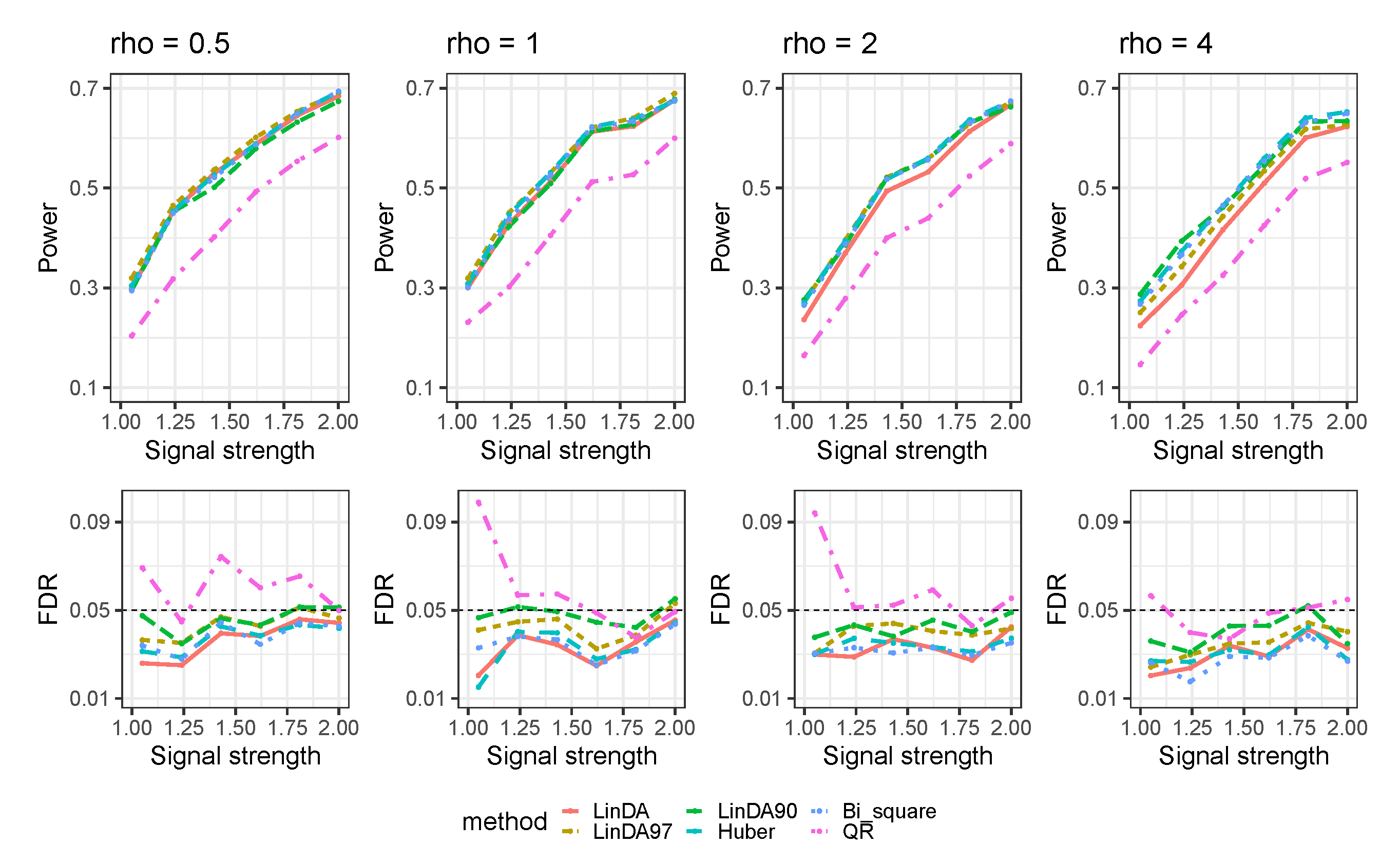
3.1.1. Heavy-Tailedness Setting
- Case 1: Student’s t-distribution with degrees of freedom 3.
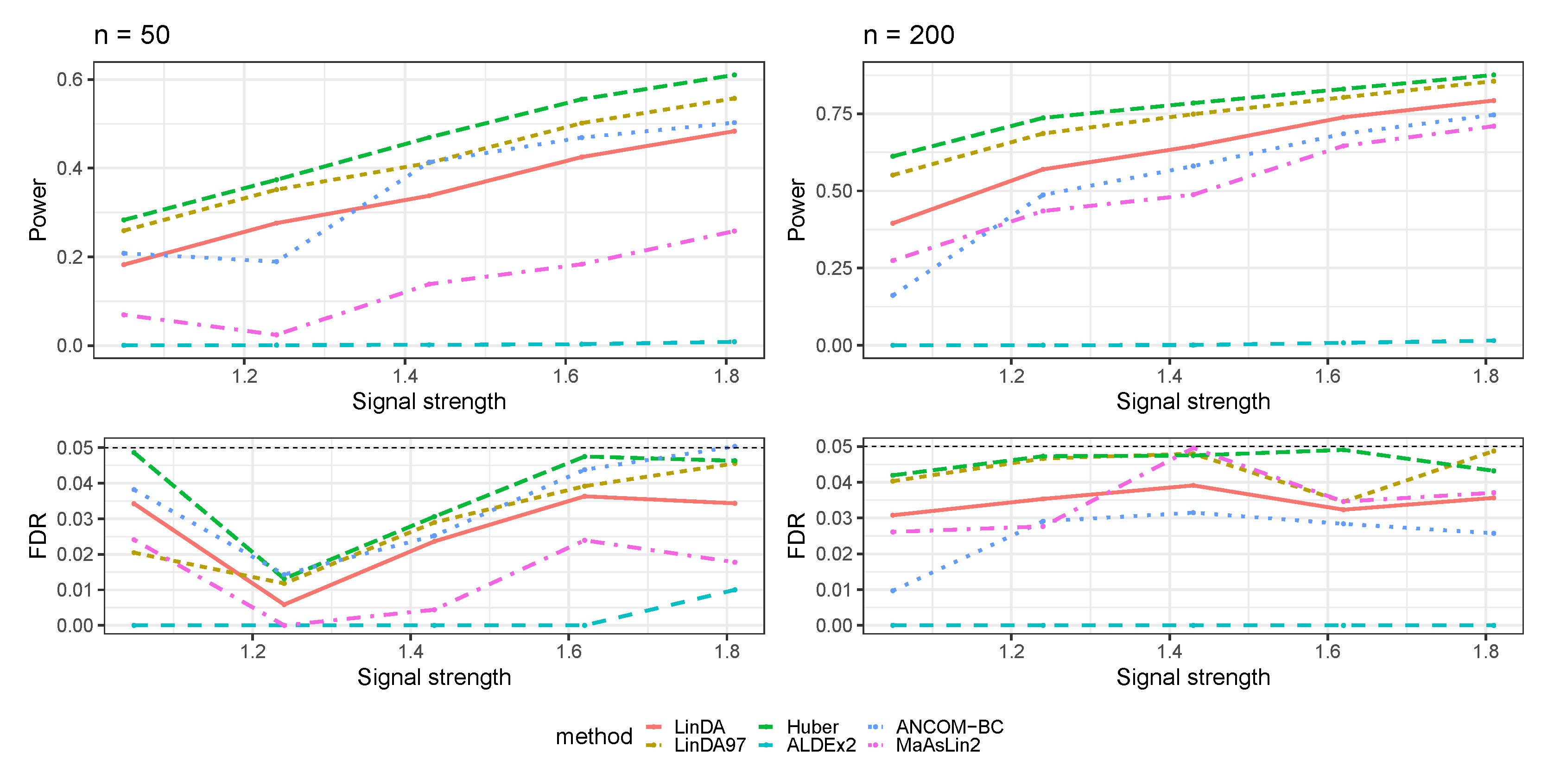
- Case 2: Log-normal distribution with log mean parameter of 0 and log standard deviation parameter of . We recentered the samples so that it has a zero mean.
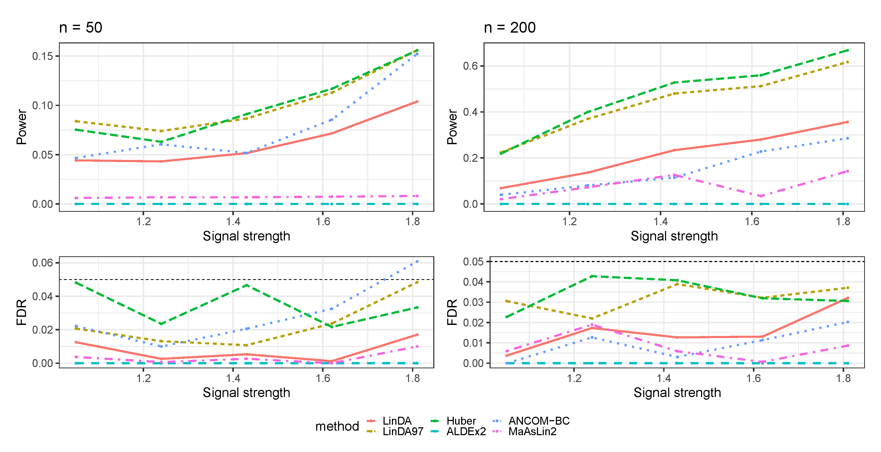
- Case 3: Weibull distribution with shape parameter of and scale parameter of . We recentered the samples so that it has a zero mean.
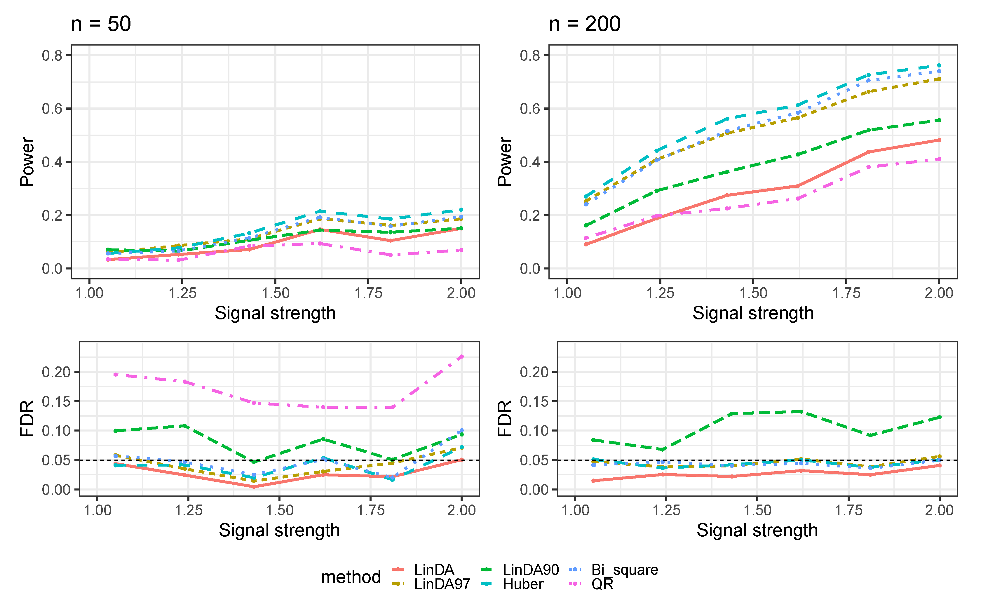
3.1.2. With Outliers Setting
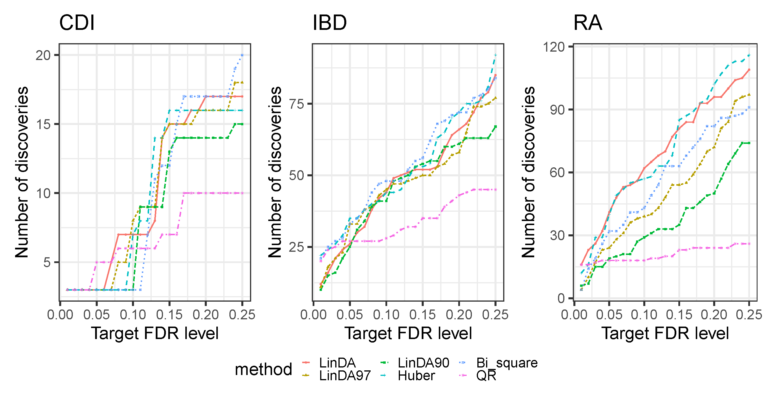
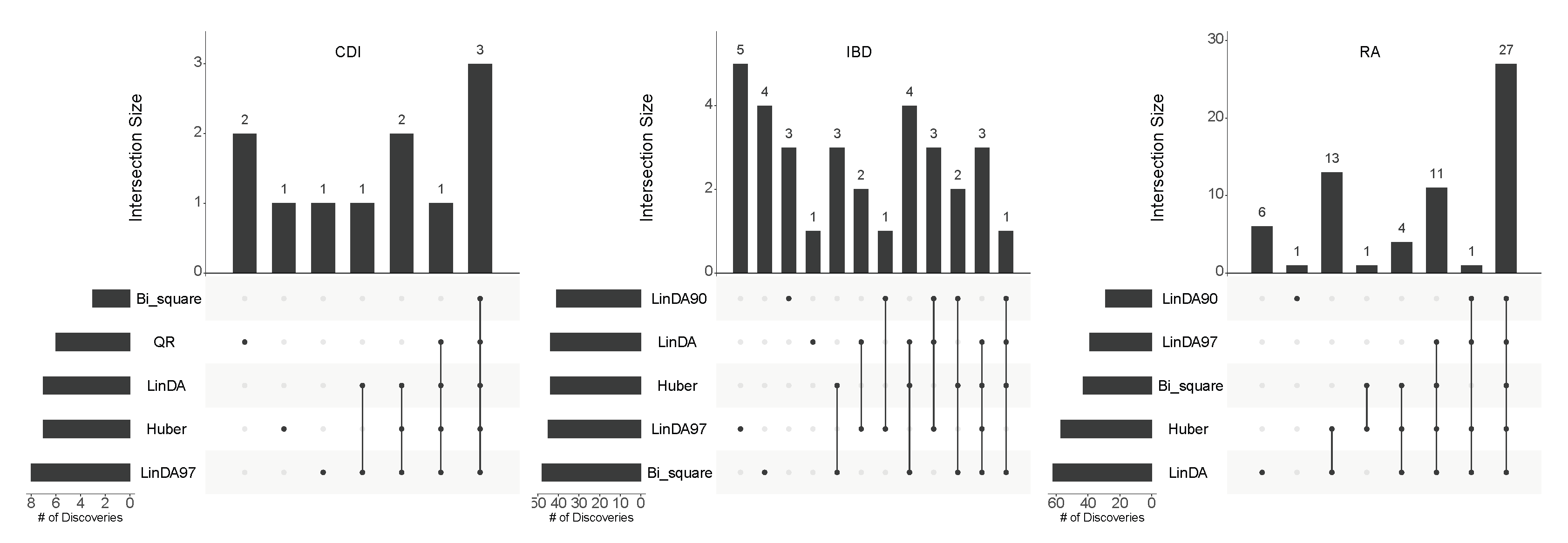
4. Real Data Analysis
5. Conclusions and Discussion
Author Contributions
Funding
Institutional Review Board Statement
Informed Consent Statement
Data Availability Statement
Conflicts of Interest
Appendix A. Additional Numerical Results for Log-Linear Model
Appendix A.1. Errors Generated Form Normal Distribution
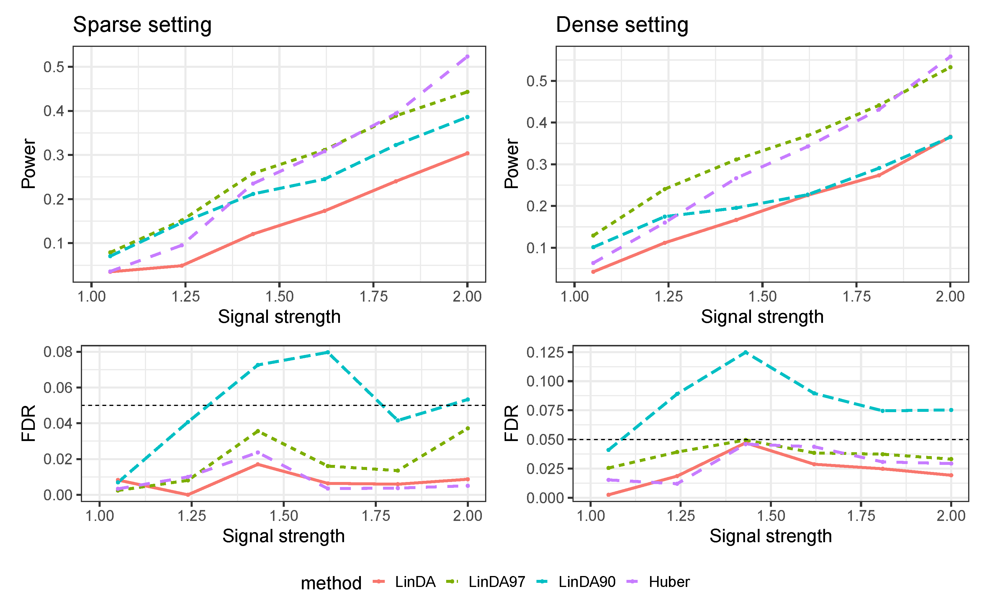
Appendix A.2. Numerical Results for Dense-Signal Setting
Appendix A.3. Numerical Results with Confounders


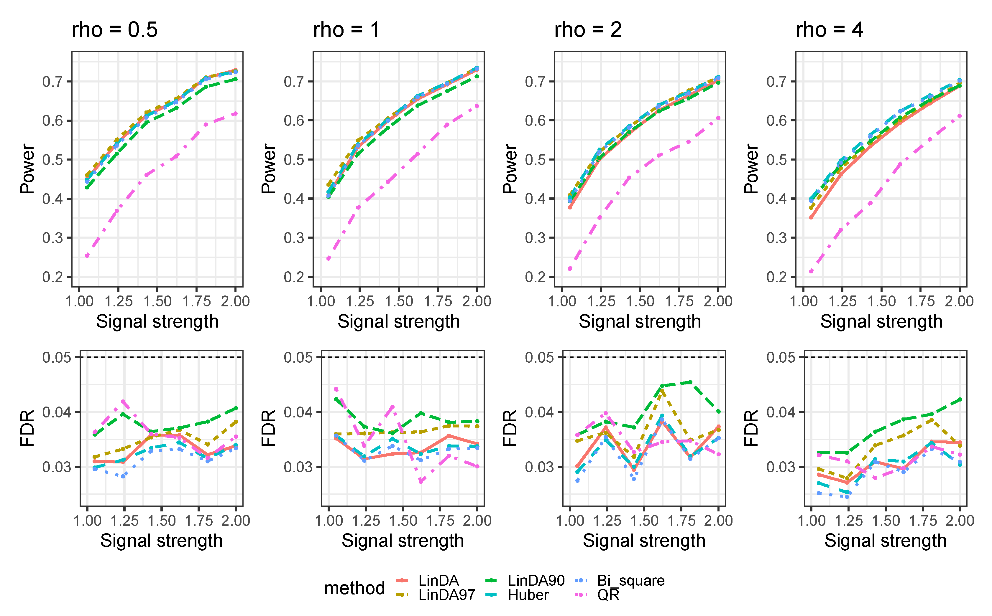
Appendix B. Mixed-Effects Models
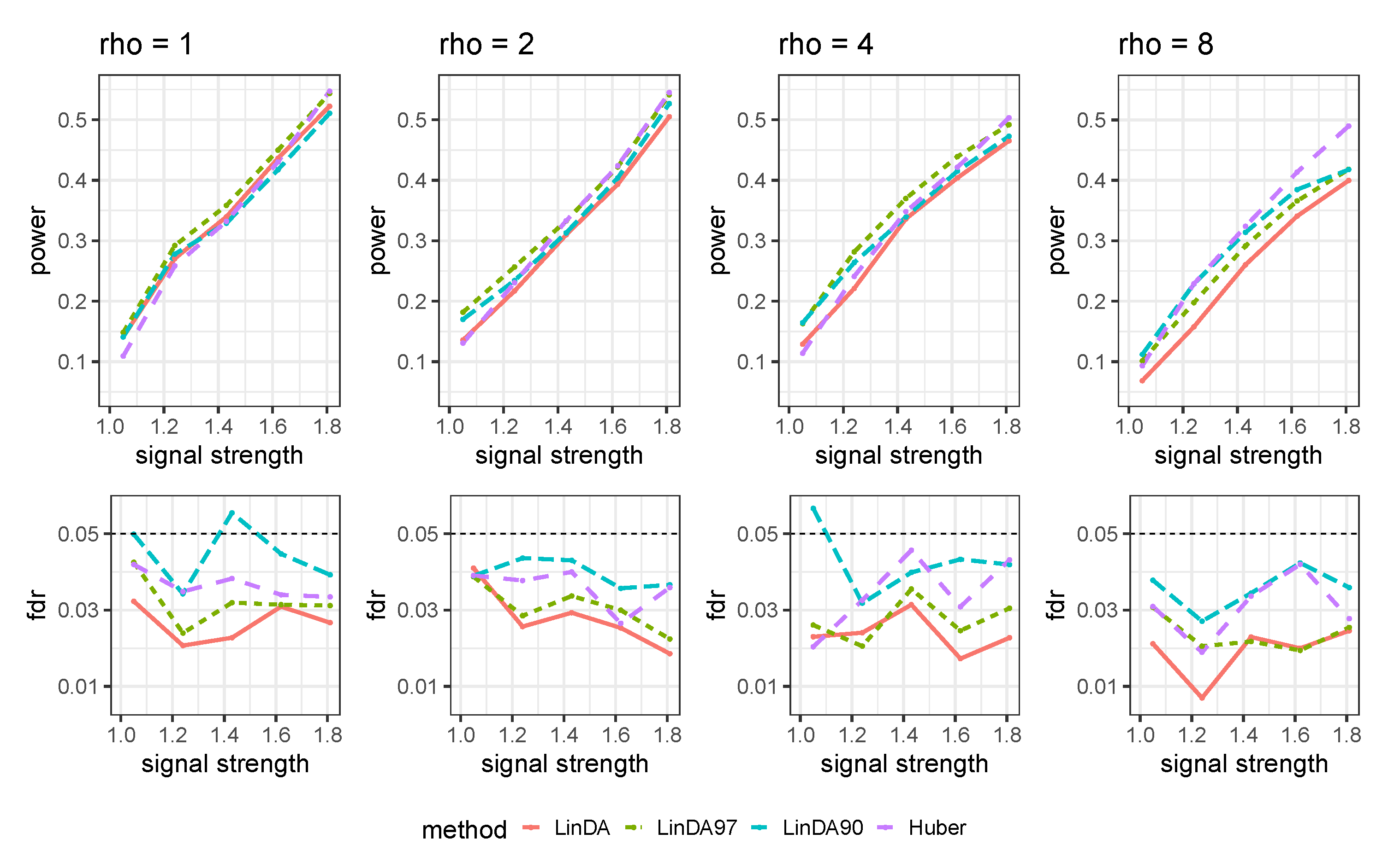
Appendix B.1. Heavy-Tailedness Setting
- 1.
- Case1: We sampled and from Log-normal distribution with log mean parameter of 0 for both terms and log standard deviation parameter of and , respectively. We recentered the samples so that it has a zero mean.
- 2.
- Case2: We sampled and from a Weibull distribution with scale parameter of for both terms and shape parameter of and , respectively. We recentered the samples so that it has a zero mean.

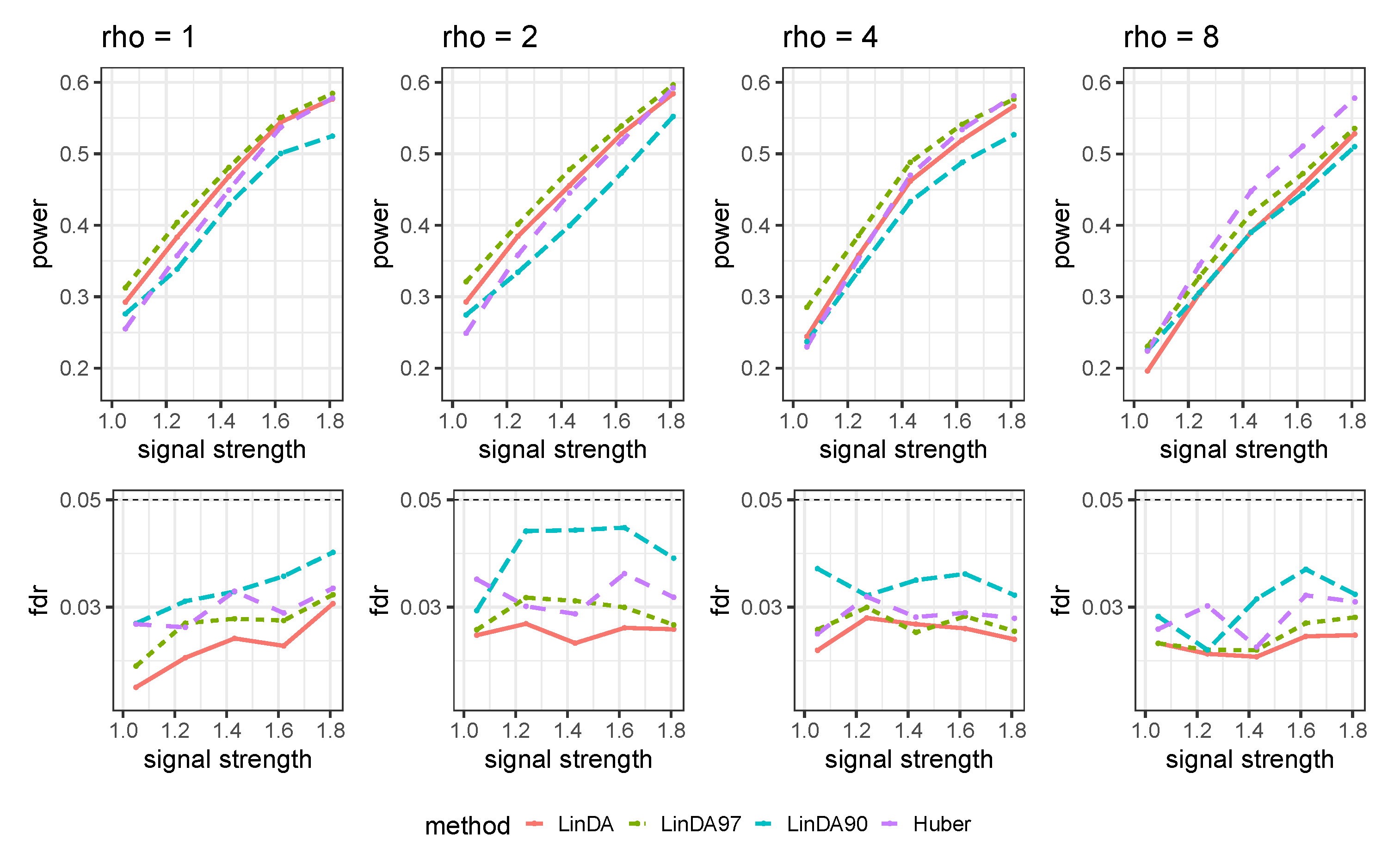
Appendix B.2. With Outliers Setting
Appendix C. Additional Numerical Results for Comparison with Other Methods

References
- Cho, I.; Blaser, M.J. The human microbiome: At the interface of health and disease. Nat. Rev. Genet. 2012, 13, 260–270. [Google Scholar] [CrossRef] [PubMed]
- Valdes, A.M.; Walter, J.; Segal, E.; Spector, T.D. Role of the gut microbiota in nutrition and health. BMJ 2018, 361, k2179. [Google Scholar] [CrossRef] [PubMed]
- Knights, D.; Lassen, K.G.; Xavier, R.J. Advances in inflammatory bowel disease pathogenesis: Linking host genetics and the microbiome. Gut 2013, 62, 1505–1510. [Google Scholar] [CrossRef] [PubMed]
- Fan, Y.; Pedersen, O. Gut microbiota in human metabolic health and disease. Nat. Rev. Microbiol. 2021, 19, 55–71. [Google Scholar] [CrossRef] [PubMed]
- Kuczynski, J.; Lauber, C.L.; Walters, W.A.; Parfrey, L.W.; Clemente, J.C.; Gevers, D.; Knight, R. Experimental and analytical tools for studying the human microbiome. Nat. Rev. Genet. 2012, 13, 47–58. [Google Scholar] [CrossRef] [PubMed]
- Truong, D.T.; Franzosa, E.A.; Tickle, T.L.; Scholz, M.; Weingart, G.; Pasolli, E.; Tett, A.; Huttenhower, C.; Segata, N. MetaPhlAn2 for enhanced metagenomic taxonomic profiling. Nat. Methods 2015, 12, 902–903. [Google Scholar] [CrossRef] [PubMed]
- Tsilimigras, M.C.; Fodor, A.A. Compositional data analysis of the microbiome: Fundamentals, tools, and challenges. Ann. Epidemiol. 2016, 26, 330–335. [Google Scholar] [CrossRef] [PubMed]
- Morton, J.T.; Marotz, C.; Washburne, A.; Silverman, J.; Zaramela, L.S.; Edlund, A.; Zengler, K.; Knight, R. Establishing microbial composition measurement standards with reference frames. Nat. Commun. 2019, 10, 2719. [Google Scholar] [CrossRef]
- Callahan, B.J.; McMurdie, P.J.; Rosen, M.J.; Han, A.W.; Johnson, A.J.A.; Holmes, S.P. DADA2: High-resolution sample inference from Illumina amplicon data. Nat. Methods 2016, 13, 581–583. [Google Scholar] [CrossRef]
- Yang, L.; Chen, J. A comprehensive evaluation of microbial differential abundance analysis methods: Current status and potential solutions. Microbiome 2022, 10, 130. [Google Scholar] [CrossRef]
- Robinson, M.D.; Oshlack, A. A scaling normalization method for differential expression analysis of RNA-seq data. Genome Biol. 2010, 11, R25. [Google Scholar] [CrossRef] [PubMed]
- Anders, S.; Huber, W. Differential expression analysis for sequence count data. Nat. Preced. 2010, 1. [Google Scholar] [CrossRef]
- Paulson, J.N.; Stine, O.C.; Bravo, H.C.; Pop, M. Differential abundance analysis for microbial marker-gene surveys. Nat. Methods 2013, 10, 1200–1202. [Google Scholar] [CrossRef] [PubMed]
- Chen, L.; Reeve, J.; Zhang, L.; Huang, S.; Wang, X.; Chen, J. GMPR: A robust normalization method for zero-inflated count data with application to microbiome sequencing data. PeerJ 2018, 6, e4600. [Google Scholar] [CrossRef] [PubMed]
- Fernandes, A.D.; Reid, J.N.; Macklaim, J.M.; McMurrough, T.A.; Edgell, D.R.; Gloor, G.B. Unifying the analysis of high-throughput sequencing datasets: Characterizing RNA-seq, 16S rRNA gene sequencing and selective growth experiments by compositional data analysis. Microbiome 2014, 2, 15. [Google Scholar] [CrossRef] [PubMed]
- Lin, H.; Peddada, S.D. Analysis of compositions of microbiomes with bias correction. Nat. Commun. 2020, 11, 3514. [Google Scholar] [CrossRef] [PubMed]
- Mallick, H.; Rahnavard, A.; McIver, L.J.; Ma, S.; Zhang, Y.; Nguyen, L.H.; Tickle, T.L.; Weingart, G.; Ren, B.; Schwager, E.H.; et al. Multivariable association discovery in population-scale meta-omics studies. PLoS Comput. Biol. 2021, 17, e1009442. [Google Scholar] [CrossRef] [PubMed]
- Zhou, H.; He, K.; Chen, J.; Zhang, X. LinDA: Linear models for differential abundance analysis of microbiome compositional data. Genome Biol. 2022, 23, 95. [Google Scholar] [CrossRef]
- Montassier, E.; Al-Ghalith, G.A.; Hillmann, B.; Viskocil, K.; Kabage, A.J.; McKinlay, C.E.; Sadowsky, M.J.; Khoruts, A.; Knights, D. CLOUD: A non-parametric detection test for microbiome outliers. Microbiome 2018, 6, 137. [Google Scholar] [CrossRef]
- Chen, J.; King, E.; Deek, R.; Wei, Z.; Yu, Y.; Grill, D.; Ballman, K. An omnibus test for differential distribution analysis of microbiome sequencing data. Bioinformatics 2018, 34, 643–651. [Google Scholar] [CrossRef]
- Nearing, J.T.; Douglas, G.M.; Hayes, M.G.; MacDonald, J.; Desai, D.K.; Allward, N.; Jones, C.M.; Wright, R.J.; Dhanani, A.S.; Comeau, A.M.; et al. Microbiome differential abundance methods produce different results across 38 datasets. Nat. Commun. 2022, 13, 342. [Google Scholar] [CrossRef] [PubMed]
- Huber, P.J. Robust regression: Asymptotics, conjectures and Monte Carlo. Ann. Stat. 1973, 1, 799–821. [Google Scholar] [CrossRef]
- Dixon, W.J.; Yuen, K.K. Trimming and winsorization: A review. Stat. Hefte 1974, 15, 157–170. [Google Scholar] [CrossRef]
- Kimura, D.K. Analyzing relative abundance indices with log-linear models. N. Am. J. Fish. Manag. 1988, 8, 175–180. [Google Scholar] [CrossRef]
- Rivest, L.P.; Lévesque, T. Improved log-linear model estimators of abundance in capture-recapture experiments. Can. J. Stat. 2001, 29, 555–572. [Google Scholar] [CrossRef]
- Fox, J.; Weisberg, S. Robust regression. R S-Plus Companion Appl. Regres. 2002, 91, 6. [Google Scholar]
- Van der Vaart, A.W. Asymptotic Statistics; Cambridge University Press: Cambridge, UK, 2000; Volume 3. [Google Scholar]
- Liu, Y.; Chen, S.; Li, Z.; Morrison, A.C.; Boerwinkle, E.; Lin, X. ACAT: A fast and powerful p value combination method for rare-variant analysis in sequencing studies. Am. J. Hum. Genet. 2019, 104, 410–421. [Google Scholar] [CrossRef] [PubMed]
- Fan, J.; Li, Q.; Wang, Y. Estimation of high dimensional mean regression in the absence of symmetry and light tail assumptions. J. R. Stat. Soc. Ser. B Stat. Methodol. 2017, 79, 247. [Google Scholar] [CrossRef]
- Schubert, A.M.; Rogers, M.A.; Ring, C.; Mogle, J.; Petrosino, J.P.; Young, V.B.; Aronoff, D.M.; Schloss, P.D. Microbiome data distinguish patients with Clostridium difficile infection and non-C. difficile-associated diarrhea from healthy controls. mBio 2014, 5, e01021-14. [Google Scholar] [CrossRef]
- Morgan, X.C.; Tickle, T.L.; Sokol, H.; Gevers, D.; Devaney, K.L.; Ward, D.V.; Reyes, J.A.; Shah, S.A.; LeLeiko, N.; Snapper, S.B.; et al. Dysfunction of the intestinal microbiome in inflammatory bowel disease and treatment. Genome Biol. 2012, 13, R79. [Google Scholar] [CrossRef]
- Gonzalez, A.; Navas-Molina, J.A.; Kosciolek, T.; McDonald, D.; Vázquez-Baeza, Y.; Ackermann, G.; DeReus, J.; Janssen, S.; Swafford, A.D.; Orchanian, S.B.; et al. Qiita: Rapid, web-enabled microbiome meta-analysis. Nat. Methods 2018, 15, 796–798. [Google Scholar] [CrossRef]
- Lex, A.; Gehlenborg, N.; Strobelt, H.; Vuillemot, R.; Pfister, H. UpSet: Visualization of intersecting sets. IEEE Trans. Vis. Comput. Graph. 2014, 20, 1983–1992. [Google Scholar] [CrossRef]
- Koller, M. robustlmm: An R package for robust estimation of linear mixed-effects models. J. Stat. Softw. 2016, 75, 1–24. [Google Scholar] [CrossRef]
- Halekoh, U.; Højsgaard, S. A kenward-roger approximation and parametric bootstrap methods for tests in linear mixed models—The R package pbkrtest. J. Stat. Softw. 2014, 59, 1–32. [Google Scholar] [CrossRef]

Disclaimer/Publisher’s Note: The statements, opinions and data contained in all publications are solely those of the individual author(s) and contributor(s) and not of MDPI and/or the editor(s). MDPI and/or the editor(s) disclaim responsibility for any injury to people or property resulting from any ideas, methods, instructions or products referred to in the content. |
© 2023 by the authors. Licensee MDPI, Basel, Switzerland. This article is an open access article distributed under the terms and conditions of the Creative Commons Attribution (CC BY) license (https://creativecommons.org/licenses/by/4.0/).
Share and Cite
Li, G.; Yang, L.; Chen, J.; Zhang, X. Robust Differential Abundance Analysis of Microbiome Sequencing Data. Genes 2023, 14, 2000. https://doi.org/10.3390/genes14112000
Li G, Yang L, Chen J, Zhang X. Robust Differential Abundance Analysis of Microbiome Sequencing Data. Genes. 2023; 14(11):2000. https://doi.org/10.3390/genes14112000
Chicago/Turabian StyleLi, Guanxun, Lu Yang, Jun Chen, and Xianyang Zhang. 2023. "Robust Differential Abundance Analysis of Microbiome Sequencing Data" Genes 14, no. 11: 2000. https://doi.org/10.3390/genes14112000
APA StyleLi, G., Yang, L., Chen, J., & Zhang, X. (2023). Robust Differential Abundance Analysis of Microbiome Sequencing Data. Genes, 14(11), 2000. https://doi.org/10.3390/genes14112000