Article

Using Sequence Similarity Based on CKSNP Features and a Graph Neural Network Model to Identify miRNA–Disease Associations

1
College of Biomedical Engineering, Sichuan University, Chengdu 610065, China
2
College of Biology, Southwest Jiaotong University, Chengdu 611756, China
3
College of Biology, Georgia State University, Atlanta, GA 30302-3965, USA
*
Author to whom correspondence should be addressed.
These authors contributed equally to this work.
Genes 2022, 13(10), 1759; https://doi.org/10.3390/genes13101759
Submission received: 4 August 2022 / Revised: 25 September 2022 / Accepted: 26 September 2022 / Published: 28 September 2022
(This article belongs to the Special Issue Identification of Potential Links in Biomedical Networks)

Abstract

:
Among many machine learning models for analyzing the relationship between miRNAs and diseases, the prediction results are optimized by establishing different machine learning models, and less attention is paid to the feature information contained in the miRNA sequence itself. This study focused on the impact of the different feature information of miRNA sequences on the relationship between miRNA and disease. It was found that when the graph neural network used was the same and the miRNA features based on the K-spacer nucleic acid pair composition (CKSNAP) feature were adopted, a better graph neural network prediction model of miRNA–disease relationship could be built (AUC = 93.71%), which was 0.15% greater than the best model in the literature based on the same benchmark dataset. The optimized model was also used to predict miRNAs related to lung tumors, esophageal tumors, and kidney tumors, and 47, 47, and 37 of the top 50 miRNAs related to three diseases predicted separately by the model were consistent with descriptions in the wet experiment validation database (dbDEMC).

1. Introduction

According to molecular biology, the entire human genome can be divided into regulatory, coding, and noncoding genes. The coding genes are the main carriers of human genetic information, accounting for only 1.5% of the whole human genome [1,2,3]. Previous studies have regarded non-coding genes as transcriptional noise in the coding process. However, microarray experiments have found that non-coding genes can participate in cell activities by interacting with proteins and DNA, affecting gene activation and silencing; RNA splicing, modification, and editing; and protein translation, thus affecting various physiological processes. MicroRNA (miRNA) is a type of non-coding, single-stranded RNA encoded by endogenous genes. The most common role of miRNA is to directly regulate target genes by affecting post-transcriptional gene regulation of promoters. Abnormal expression of miRNA can cause many human diseases, and miRNA can be used as a drug target for disease treatment [4,5]. Therefore, the regulatory role of miRNA in disease expression is significant for a variety of complex human physiological processes and disease pathophysiology. However, traditional experimental methods are often limited. To this end, it is of great significance to speed up the verification process, reduce bias in biological experiments, and establish a method to predict the possible associations quickly and effectively between miRNAs and disease [6].
Common biological experimental methods from the 1990s to the beginning of the 21st century include reverse transcription-polymerase chain reaction (RT-PCR) [7], Northern blotting [8], and microarray profiling [9]. Although these traditional methods can accurately detect correlations between miRNA and disease, they have their limitations. In recent years, a more classical class of algorithm has been developed based on the assumption of similarity measures [10]. This kind of algorithm is based on the assumption that miRNAs with similar functions are also related to similar disease phenotypes and can be sequenced accordingly [11]. Jiang et al. [12] constructed an miRNA association network using probability of interaction by target accessibility (PITA), and they proposed a hypergeometric distribution prediction method based on the human miRNA network. Liu et al. [13] proposed an miRNA–disease association prediction method by random walk on a heterogeneous network constructed by integrating multiple data sources. Zeng et al. [14] applied a link prediction algorithm named the structural perturbation method (SPM) on the miRNA–disease bilayer network to predict potential miRNA–disease associations. Zhang et al. [15] proposed a method using the correlation spectrum and the interaction network between miRNA and target genes to calculate the miRNA–disease association score by using fast linear neighborhood similarity-based network link inference. Mørk et al. [16] proposed a model to calculate the similarity between miRNA and disease based on the distance between target genes and disease genes in the PPI network. Another common method for predicting the miRNA–disease association is based on machine-inferred code similarity (MISIM) proposed by Wang et al. [17] Chen et al. [18] proposed a model called random forest for miRNA–disease association (RFMDA), which integrates disease semantic similarity, disease Gaussian interaction profile kernel similarity, miRNA Gaussian interaction profile kernel similarity, and miRNA functional similarity based on MISIM to predict miRNA–disease association. Zeng et al. [19] developed a neural network model to predict miRNA–disease associations (NNMDA). NNMDA not only aggregated the neighbor information during the process, but also preserved the topology of the original network at the same time. Zhou et al. [20] used similar methods to obtain miRNA and disease similarity networks and used the gradient boosting decision tree (GBDT) algorithm to extract more representative features. Additionally, with the recent great progress of graph neural networks in processing graph data, prediction methods based on graph neural networks have made breakthroughs, and the association between miRNA and disease is more suited to using graph neural networks than other data structures.
A key step in the data preprocessing for all models is to calculate the similarity of miRNAs. Specifically, these methods can be divided into three types: similarity measure-based methods, MISIM-based methods, and miRNA sequence similarity-based methods. Similarity measure-based methods construct an miRNA association network using target gene associations. However, this depends on the association between miRNA and target genes, resulting in high false positive and false negative rates [12,15,16,21,22,23,24,25,26,27,28]. The MISIM-based methods construct an miRNA association network using a disease semantic similarity network [17]. It can be said that related miRNAs have related diseases, but not all miRNAs related to similar diseases are necessarily related [18,20,28,29,30]. The miRNA similarity networks of such methods have the disadvantage of being dependent on known disease similarity networks, and this error is more pronounced for miRNAs that are associated with fewer diseases. The sequence similarity of miRNA is also particularly important for similarity networks. Previous studies have proposed enriching the miRNA similarity networks using miRNA sequence information. Ji et al. [31] integrated various kinds of information to construct a heterogeneous network centered on miRNA and disease, and embedded K-mer sequence features of miRNA into this network. Ji et al. [32] proposed a method using disease semantic similarity and miRNA sequence similarity to construct an miRNA–disease association network; miRNA sequence similarity-based methods effectively quantify the miRNA similarity, solving the problem that miRNA sequences cannot be directly compared due to their different lengths. In conclusion, according to current research, there is still room for improvement in the accuracy and effectiveness of identifying and predicting potential associations between miRNA and disease. Therefore, we enhanced the effective associations between miRNA and disease by using miRNA sequence information, benefitting from the advantage of graph neural networks in finding miRNA–disease associations to construct a feature extraction method based on miRNA sequence similarity information.
In this study, we propose a method to calculate the sequence characteristics and sequence similarity of miRNA using five distinct miRNA sequence characteristics. Then, by integrating disease semantic similarity, miRNA Gaussian interaction profile kernel similarity, and disease Gaussian interaction profile kernel similarity, we construct a new bipartite graph of miRNA and disease. Then, the auto-encoder of a graph neural network is used to predict miRNA–disease association. Moreover, we evaluated prediction performance using 5-fold cross-validation. The model, using sequence similarity based on the composition of k-spaced nucleic acid pair (CKSNAP) features and a graph neural network, achieved an average area under the curve (AUC) of 93.71 ± 0.42%, with an accuracy of 83.69 ± 1.42%, precision of 77.73 ± 2.29%, recall of 94.62 ± 0.97%, and F1-score of 85.31 ± 1.00%. To further verify the performance of this model, case studies on lung, esophageal, and kidney neoplasms were conducted. Respectively, the results showed that 47, 47, and 37 of the top 50 predicted miRNAs for these neoplasms can be confirmed by the database of Differentially Expressed MiRNAs in human Cancers (dbDEMC) [33]. In conclusion, it can be inferred that our model is effective and accurate in identifying potential associations between miRNA and disease.

2. Materials and Methods

2.1. Human miRNA–Disease Associations

In this study, we adopted the Human microRNA Disease Database (HMDD; v3.2) as the benchmark dataset and directly downloaded the experimentally verified miRNA–disease associations from https://www.cuilab.cn/hmdd (accessed on 1 September 2021) [34]. There are 16,427 high-quality miRNA–disease associations recorded in the HMDD database, including 877 diseases and 901 miRNAs. We adopted the adjacency matrix A to quantify associations between these miRNAs and diseases. If a disease is associated with an miRNA, the value of the element at the corresponding position of matrix A is set to 1, and otherwise to 0.

2.2. miRNA Sequence Similarity

In this study, the attribute features of miRNAs were represented by sequence similarity information. We downloaded miRNA sequence information from https://mirbase.org/ftp.shtml and utilized the K-mer (k = 3), Moran, Geary, NMBroto, and CKSNAP (k = 5) methods to obtain the sequence features of miRNAs.
K-mer: We set up a sliding window with a size of 3 and a sliding distance of 1 to obtain occurrence frequencies for all 3-monomere units. Then, each miRNA sequence was converted into a 64-dimensional vector based on the 64 3-monomer combinations. On this basis, we used cosine similarity, euclidean distance, and the Pearson correlation coefficient to calculate miRNA sequence similarity, defined as follows:
K m e r _ cos _ s i m ( i ,   j ) = j = 1 n i = 1 n N ( i ) N × N ( j ) N i = 1 n ( N ( i ) N ) 2 × j = 1 n ( N ( j ) N ) 2  
K m e r _ e u c _ d i s t ( i , j ) = i = 1 j = 1 n ( N ( i ) N N ( j ) N ) 2  
K m e r _ p e a r s o n ( i , j ) = N N ( i ) N × N ( j ) N N ( i ) N N ( j ) N N ( N ( i ) N ) 2 ( N ( i ) N ) 2 N ( N ( j ) N ) 2 ( N ( j ) N ) 2
where i represents a nucleotide combination with a length of three, such as AAA, AAC, and AAG; N(i) is the number of nucleotide combinations and N is the length of a nucleotide sequence.
Moran: Moran describes miRNA by physicochemical parameters of nucleotides. The physical and chemical properties of miRNA include Rise (RNA), Roll(RNA), Shift(RNA), Slide(RNA), Tilt(RNA), Twist(RNA), Entropy(RNA), Adenine content, Purine(AG) content, Hydrophilicity(RNA), Enthalpy(RNA)1, GC content, Entropy(RNA)1, Hydrophilicity(RNA)1, Free energy(RNA), Keto(GT) content, Free energy(RNA)1, Enthalpy(RNA), Stacking energy(RNA), Guanine content, Cytosine content, and Thymine content. On this basis, we calculated the miRNA sequence similarity, defined as follows:
M o r a n _ cos _ s i m ( i ,   j ) = j = 1 n i = 1 n M i × M j i = 1 n ( M i ) 2 × j = 1 n ( M j ) 2
M o r a n _ e u c _ d i s t ( i , j ) = i = 1 j = 1 n ( M i M j ) 2
M o r a n _ p e a r s o n ( i , j ) = N M i × M j M i M j N M i 2 ( M i ) 2 N M j 2 ( M j ) 2  
where the Moran feature of miRNA are defined as follows:
M ( d ) = 1 N d i = 1 N d ( M i M ¯ ) ( M i + d M ¯ ) 1 N i = 1 N ( M i M ¯ ) 2 ,   d = 1 , 2 , 3 , ,   n l a g
M = r = 1 l e n M r M ¯ 1 l e n r = 1 l e n ( M r M ) 2 l e n
where d represents the lag value of autocorrelation, and nlag represents the maximum value of lag. In this study, the lag value d = 3 was selected; M i is the nucleotide properties at position i. M ¯ is calculated as follows:
M ¯ = i = 1 N M i N  
Geary: Geary uses the attribute information of nucleotides to describe the sequence characteristics of miRNA. We calculate the miRNA sequence similarity, defined as follows:
G e a r y _ cos _ s i m ( i ,   j ) = j = 1 n i = 1 n G ( d ) i × G ( d ) j i = 1 n ( G ( d ) i ) 2 × j = 1 n ( G ( d ) j ) 2
G e a r y _ e u c _ d i s t ( i , j ) = i = 1 j = 1 n ( G ( d ) i G ( d ) j ) 2
G e a r y _ p e a r s o n ( i , j ) = N G ( d ) i × G ( d ) j G ( d ) i G ( d ) j N G ( d ) i 2 ( G ( d ) i ) 2 N G ( d ) j 2 ( G ( d ) j ) 2  
where the Geary feature of miRNA are defined as follows:
G ( d ) = 1 2 ( N d ) i = 1 N d ( M i M i + d ) 2 1 N 1 i = 1 N ( M i M ¯ ) 2 ,   d = 1 , 2 , , n l a g
The meaning of physical and chemical indicators involving nucleotides, such as d, M, Mi, and nlag, is the same as that in the Moran autocorrelation descriptor.
NMBroto: NMBroto is a normalized Moreau-Broto autocorrelation descriptor. The miRNA sequence is calculated similarity, defined as follows:
N M B r o t o _ cos _ s i m ( i ,   j ) = j = 1 n i = 1 n N M B ( d ) i × N M B ( d ) j i = 1 n ( N M B ( d ) i ) 2 × j = 1 n ( N M B ( d ) j ) 2  
N M B r o t o _ e u c _ d i s t ( i , j ) = i = 1 j = 1 n ( N M B ( d ) i N M B ( d ) j ) 2  
N M B r o t o _ p e a r s o n ( i , j ) = N N M B ( d ) i × N M B ( d ) j N M B ( d ) i N M B ( d ) j N N M B ( d ) i 2 ( N M B ( d ) i ) 2 N N M B ( d ) j 2 ( N M B ( d ) j ) 2
where the NMBroto feature of miRNA is defined as follows:
N M B ( d ) = i = 1 N d M i × M i + d N d ,   d = 1 , 2 , , n l a g
The meaning of physical and chemical indicators involving nucleotides, such as d, M, Mi, and nlag, is the same as that in the Moran autocorrelation descriptor.
CKSNAP: CKSNAP uses k-spaced nucleic acid pairs to describe the frequency of separating the current nucleic acid pair from any k nucleic acids. When k = 0, there are 16 pairs of nucleic acid pairs with 0 spacing (‘AA’, ‘AC’, ‘AG’, ‘AT’, ‘CA’, ‘CC’, ‘CG’, ‘CT’, ‘GA’, ‘GC’, ‘GG’, ‘GT’, ‘TA’, ‘TC’, ‘TG’, ‘TT’). The miRNA sequence was calculated similarity, defined as follows:
C K S N A P _ cos _ s i m ( i ,   j ) = j = 1 n i = 1 n C K i × C K j i = 1 n ( C K i ) 2 × j = 1 n ( C K j ) 2  
C K S N A P _ e u c _ d i s t ( i , j ) = i = 1 j = 1 n ( C K i C K j ) 2  
C K S N A P _ p e a r s o n ( i , j ) = N C K i × C K j C K i C K j N C K i 2 ( C K i ) 2 N C K j 2 ( C K j ) 2
where the CKSNAP features of miRNA are defined as follows:
C K = ( N A A N t o t a l ,   N A C N t o t a l ,   N A G N t o t a l , ,   N T T N t o t a l , ) 16
Using five miRNA sequence features and three similarity calculation methods, 15 miRNA sequence similarity matrices could be obtained. In the following research, all sequence similarity matrices are called MSSM.

2.3. Disease Semantic Similarity

Disease semantic similarity can be calculated based on the medical subject heading (MeSH) descriptors, which are available at https://www.ncbi.nlm.nih.gov (accessed on 1 January 2021). The relationship between diseases can be represented as a directed acyclic graph (DAG) network according to disciplines or affiliations, where the nodes represent the MeSH descriptors of diseases, and the directed edges point from parent nodes to child nodes [35]. We adopted D A G d i ( d k ) to describe semantic contribution of disease dk to disease di. On this basis, the semantic contribution is defined as follows:
D A G d i ( d k ) = { 1 ,   i f   d k = d i m a x { Δ D A G d i ( d k ) | d k c h i l d r e n   o f   d k } ,   i f   d k d i
where ∆ is the semantic contribution attenuation facto; this was set to 0.5 according to a previous study [30]. The semantic contribution value will decrease with distance.
According to the semantic contribution value of disease nodes, the semantic value of disease di was calculated as follows:
D V ( d i ) = d k N ( d i ) D A G d i ( d k )  
The semantic similarity between disease di and disease dk could be calculated by the nodes shared by the two disease DAG networks. It was defined as follows:
S S M ( d i , d j ) = ( D A G d i ( d t ) + D A G d j ( d t ) ) d t N ( d i ) N ( d j )   D V ( d i ) + D V ( d j )  
where the element DSSM(di, dj) represents the disease semantic similarity between di and dj.

2.4. Gaussian Interaction Profile Kernel Similarity for miRNAs and Diseases

In this study, the binary vector IP(mi) to denote the interaction profiles of miRNA mi was defined by calculating the correlation between mi and mj. The miRNA Gaussian interaction profile kernel similarity matrix (MGSM) could be calculated as follows:
M G S M ( m i , m j ) = exp ( σ m I P ( m i ) I P ( m j ) 2 )
where σm was applied for controlling the bandwidth of the kernel, and I P ( m i ) I P ( m j ) 2 was applied for calculating the euclidean distance of two eigenvectors. The Gaussian kernel bandwidth control parameter was calculated as follows:
σ m = σ m / ( 1 n m i = 1 n m I P ( m i ) 2 )
where nm represents the number of all miRNAs; σ m was set to 1 according to a previous study [30]. Similarly, the Gaussian interaction profile kernel similarity for diseases DGSM(di,dj) between disease di and dj could be calculated as follows:
D G S M ( d i , d j ) = exp ( σ d I P ( d i ) I P ( d j ) 2 )
σ d = σ d / ( 1 n d i = 1 n d I P ( d i ) 2 )
where nd represents the number of all diseases, σ d was set to 1 according to a previous study [30].

2.5. Integrated Similarity for miRNAs and Diseases

There is a large number of sparse values in the miRNA sequence similarity and disease semantic similarity matrices. The final integrated similarity for miRNAs and diseases was obtained from miRNA sequence similarity, disease semantic similarity, Gaussian interaction profile kernel similarity for miRNAs, and Gaussian interaction profile kernel similarity for diseases. It was defined as follows:
M S i m ( m i , m j ) = { M S S M ( m i , m j ) ,   i f   m i   a n d   m j   h a v e   s e q u e n c e   s i m i l a r i t y M G S M ( m i , m j ) ,   o t h e r w i s e
D S i m ( d i , d j ) = { D S S M ( d i , d j ) ,   i f   d i   a n d   d j   h a v e   s e m a n t i c   s i m i l a r i t y   D G S M ( d i , d j ) ,   o t h e r w i s e

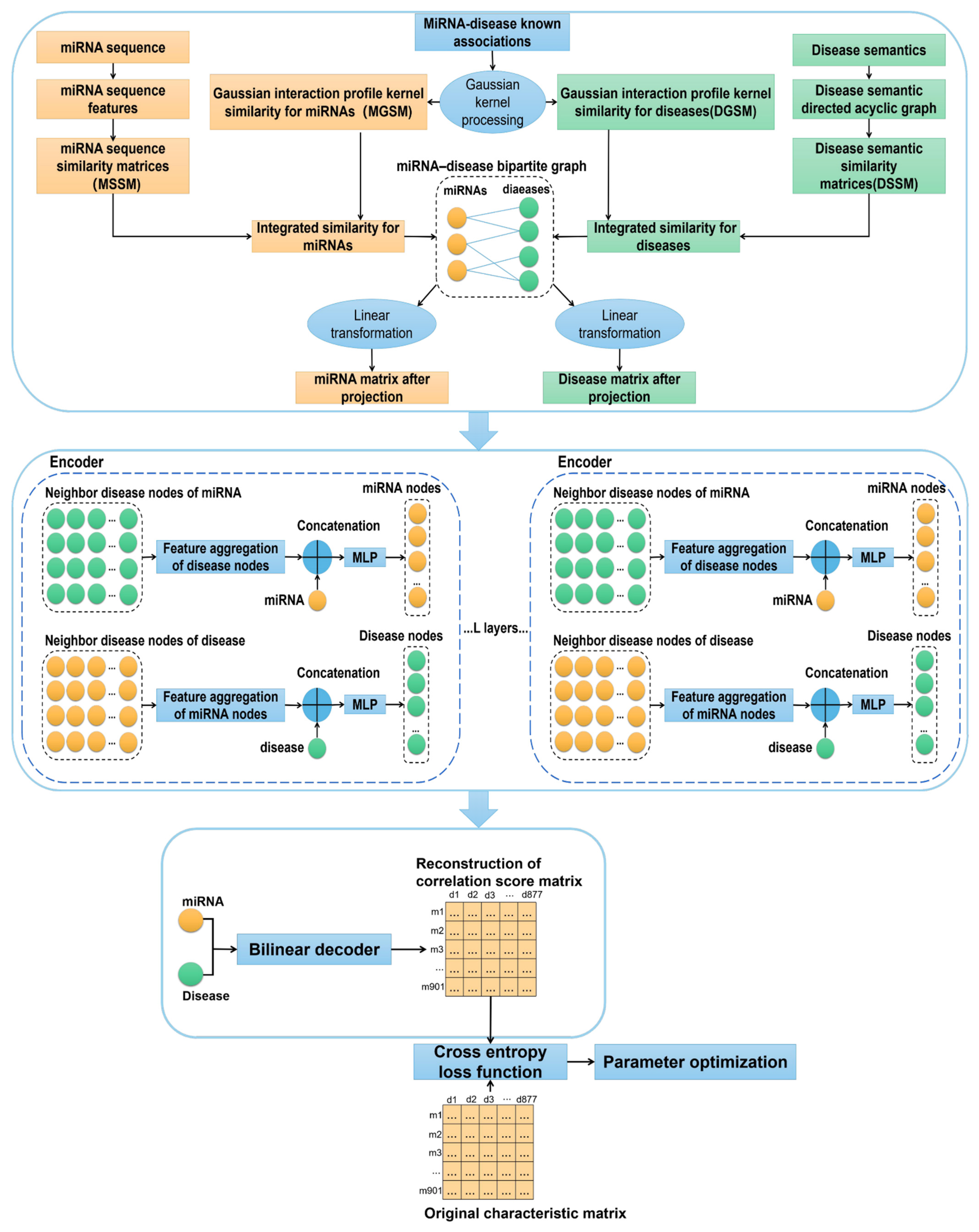
2.6. Graph Auto-Encoder

In the present study, the prediction of the potential miRNA–disease associations was mainly used to generate the low-dimensional embedding of node information through the encoder based on a graph neural network, so as to realize the identification of the correlation between miRNA and diseases by a bilinear decoder. Our model can be described in four steps, as shown in Figure 1.
First, we constructed a bipartite graph including 877 disease nodes and 901 miRNA nodes. For integrated similarity for miRNA, the similarity between miRNA mi and miRNA m1, m2, …, m901 could be expressed as follows:
F m ( i ) = ( u 1 , u 2 , u 3 , , u 901 )
where u1, u2, u3, …, u901 is the integrated similarity between miRNA m(i) and miRNA m1, m2, …, m901. Similarly, the integrated similarity between disease di and disease d1, d2, …, d901 could be expressed as follows:
F d ( i ) = ( v 1 , v 2 , v 3 , , v 877 )
The vectors in Fm (miRNA) and Fd (disease) were embedded into miRNA nodes and disease nodes in the miRNA–disease bipartite graph. In this study, 16,427 known association pairs verified by experiments were regarded as positive samples of input. In order to balance the positive and negative samples, 16,427 negative samples were randomly selected from the unknown associations in the subsequent experiments. In order to project miRNA and disease feature vectors to the same vector space, we designed a linear transformation matrix. The projection process of miRNA nodes can be described as follows:
H m = W m · F m
where Fm is the original characteristic matrix of miRNA, W m is to realize the linear transformation matrix of miRNA projection process, and Hm is the feature matrix of miRNA projected into the new feature space. Similarly, the projection process of disease nodes can be described as follows:
H d = W d · F d
where Fd, W m , and Hd are as described above.
Second, we used the aggregator function of the auto-encoder to integrate the feature representation of the node and its neighbor nodes, update the node with a multi-layer perceptron, and embed the aggregated features into the original features of the node. The aggregator function sum(·) was used to realize the feature aggregation of its neighbor nodes, as shown in Equations (35) and (36), where s u m ( H d ( 1 ) , H d ( 2 ) , ) represents the aggregation process of the disease nodes dj., which are the direct neighbors of the miRNA nodes mi; Dmi is the degree value of node mi. In order to prevent numerical instability, H m s ( i ) was used for normalization. It is the aggregation feature of the current miRNA node mi.
H m s ( i ) = 1 D m i s u m ( H d ( 1 ) , H d ( 2 ) , )
D m i = | { d j | e i j E   o r   e j i E } |
After the aggregation features of all miRNA nodes were obtained through the aggregator function, the features of all nodes were embedded and connected through the multi-layer perceptron superimposed by the L-layer, and the final embedding of nodes was generated. We used a Leaky Rectified Linear Unit (LeakyReLU) function as the activation function of the multilayer perceptron to avoid the phenomenon of neuron “death” when the input was negative. It is defined as follows:
H m ( i ) = L e a k y R e L U ( f ( H m ( i ) H m s ( i ) ) )
where H m ( i ) is the original feature of node mi, H m s ( i ) is the aggregation feature of node mi, H m ( i ) is the updated node feature, and f(·) is the single-layer multi-layer perceptron function. Similarly, we calculated the aggregation feature of the current disease node dj, the degree value of node dj, and the updated node feature of disease as in Equations (38)–(40).
H d s ( j ) = 1 D d ( j ) s u m ( H m ( 1 ) , H m ( 2 ) , )
D d ( j ) = | { m i | e i j E   o r   e j i E } |
H d ( j ) = L e a k y R e L U ( f ( H d ( j ) H d s ( j ) ) )
A multilayer overlay network could enhance the feature embedding of neighbor nodes and preserve the topology of graph data, so as to enhance the expression ability of features.
Third, considering that the number of unknown associations between miRNA and disease is much larger than the known associations, we adopted a sigmoid function as the activation function of the decoder to predict the association score between miRNA and disease. It is defined as follows:
A ^ ( i , j ) = s i g m o i d ( H d L ( j ) Q ( H m L ( i ) ) T )
where Q is the E-dimensional trainable parameter matrix, H d L ( j ) is the feature embedding of L-layer disease node dj, H m L ( i ) is the feature embedding of L-layer miRNA node mi, and A ^ ( i , j ) is the reconstructed association score matrix.
Finally, we used the deviation between the prediction score matrix and the original characteristic matrix and used the cross-entropy loss function and back propagation algorithm to optimize the model to obtain the best model parameters. It is defined as follows:
L O S S = i , j y y ( A ( i , j ) l o g A ^ ( i , j ) + ( 1 A ( i , j ) ) log ( 1 A ^ ( i , j ) ) )
where A ( i , j ) is the original characteristic matrix, and A ^ ( i , j ) is the reconstructed prediction correlation score matrix. Due to the small proportion of known associations in the sample data, cost-sensitive learning was used to improve the weight of positive sample loss, so as to improve the prediction accuracy. Furthermore, y and y- are the set of positive samples and the set of negative samples in the incidence matrix, respectively.

2.7. Model Evaluation

Five-fold cross validation was selected to evaluate the performance of the model. We divided the miRNA–disease associations into five sets, set one as the test set and the other four as the training set, and received five prediction results. Accordingly, the higher the score between miRNA and disease, the higher the possibility of a potential association between them. In the present study, we adopted four common evaluating indicators to evaluate the performance of the models: Accuracy (Acc), Precision (Prec), Recall, and F1-score. Meanwhile, we plotted the receiver operating characteristic curves to intuitively display the performance of our model and utilized the AUC to comprehensively evaluate model performance.

3. Results

3.1. Performance Evaluation of Graph Neural Network Prediction Model Based on Single Features

Based on five sequence features, we used three different similarity calculation methods to obtain 15 different miRNA sequence similarity matrices and constructed 15 prediction models. The performance comparison of the prediction models based on different characteristics and similarity calculation methods is shown in Figure 2. The overall prediction performance of the model for calculating sequence feature similarity based on the Pearson correlation coefficient was better than the other two similarity calculation methods. This type of model obtained the optimal values in AUC, ACC, precision, and F1-score, and had obvious advantages over the other two similarity algorithms. Comparing the performance of the model based on five features, we found that the performance of the model based on K-mer and CKSNAP was better than the other models. Considering that AUC could more comprehensively evaluate model performance, the model based on CKSNAP sequence features and the Pearson similarity calculation method obtained the highest AUC value among the 15 models. In addition, this model was also better than other models in ACC, precision, and F1 scores.

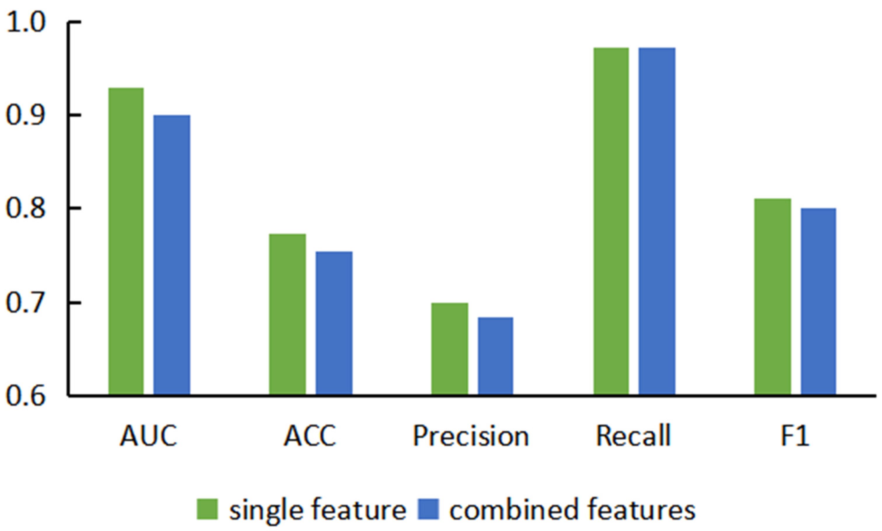
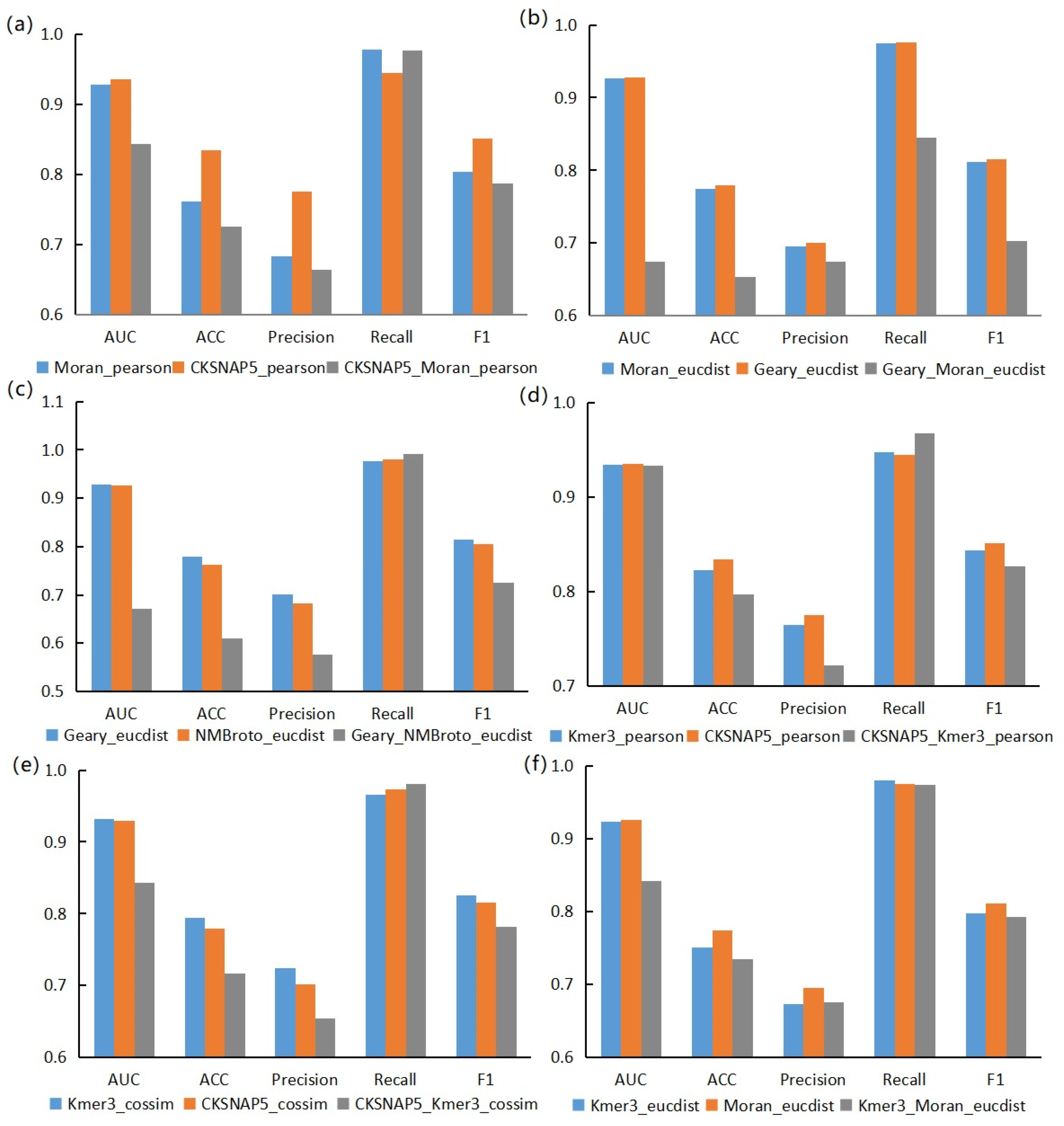
3.2. Performance Evaluation of Graph Neural Network Prediction Model Based on Combined Features

Based on the comparison and analysis of model performance based on single features, we proposed prediction models based on combined features, hoping to enhance the expression ability of nodes by embedding multiple features on a single node. Here, we combined the five features in pairs to obtain 10 combined features and used different similarity calculation methods to build 30 different prediction models based on these combined features. In order to compare the performance of the two types of models more intuitively, we classified these two types of models and calculated their average scores on each evaluation indicator and drew the prediction performance based on single-feature and double-feature models, as shown in Figure 3. We noticed that the evaluation indicators of models based on combined features were lower than those of the models based on single features. We speculate that this is because the dimensions of the combined features were too high. Embedding more feature information into a single node also introduced too much noise and redundant information, which led to model instability in the subsequent experimental process, resulting in a decline in prediction performance.
In addition, we also found that the score of the models based on combined features depended on the score of the models based on single features. Here, we selected six groups of models for display, as shown in Figure 4. It can be seen that the models based on single features were better than the models based on combined features in AUC, Acc, Prec, and F1-score. In Figure 4, the gray columns are mostly located below the other two columns. The recall rate of models based on combined features in individual groups is higher. The reason for this is that the combined features enrich the information range, which leads to the improvement of recall rate. Combined features could enrich the information contained in a single node, which would make the coverage of information and the construction of relationship structure in the whole network more comprehensive, resulting in the improvement of Recall. However, due to the high dimensions of the feature vector and too much noise information on a single node, other evaluation indicators would decline.
Based on this, the subsequent experiments focused on performance optimization based on single-feature models. In a preliminary study, we set project dimension to E = 256 and set encoder layers to L = 2.

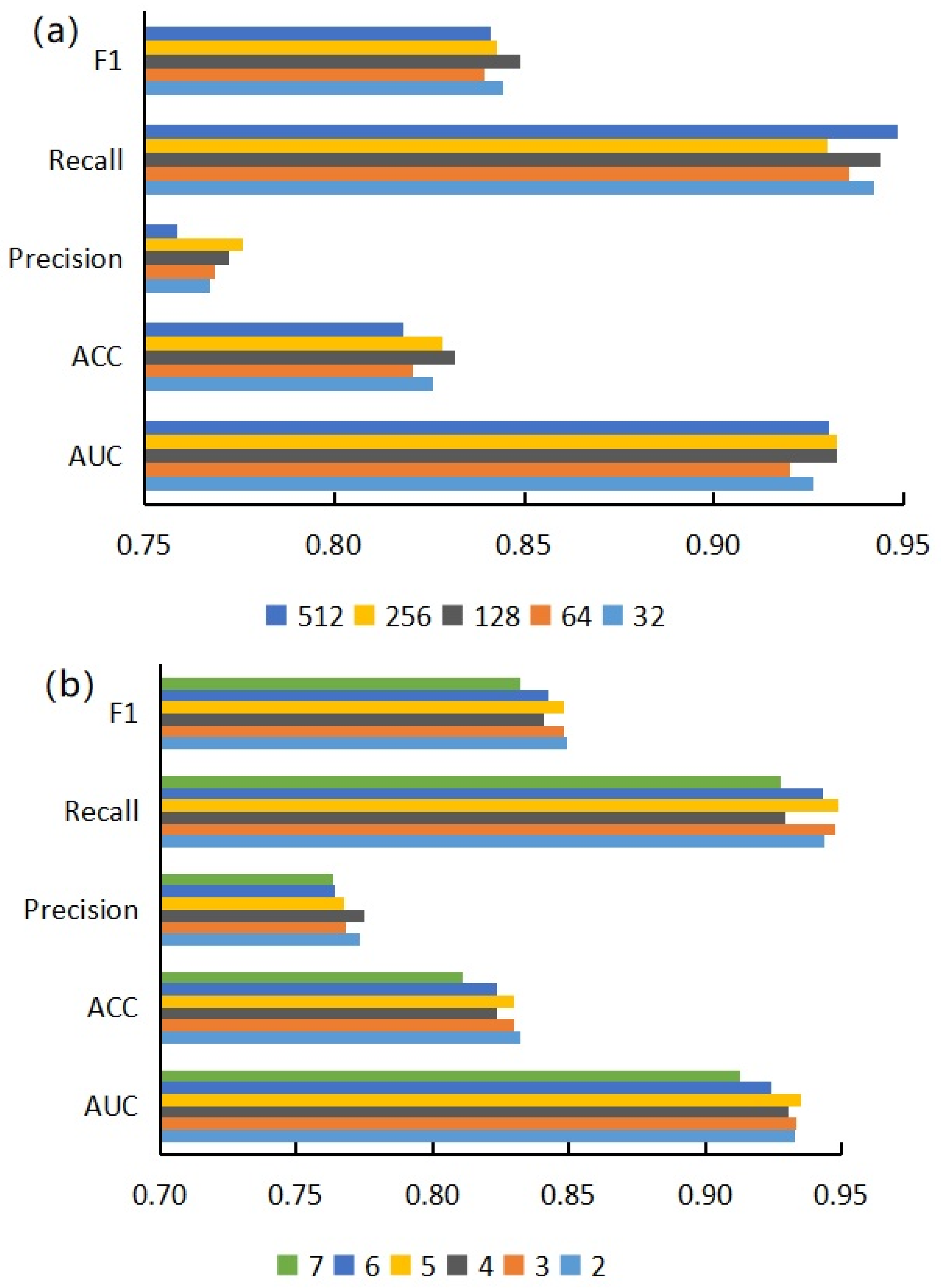
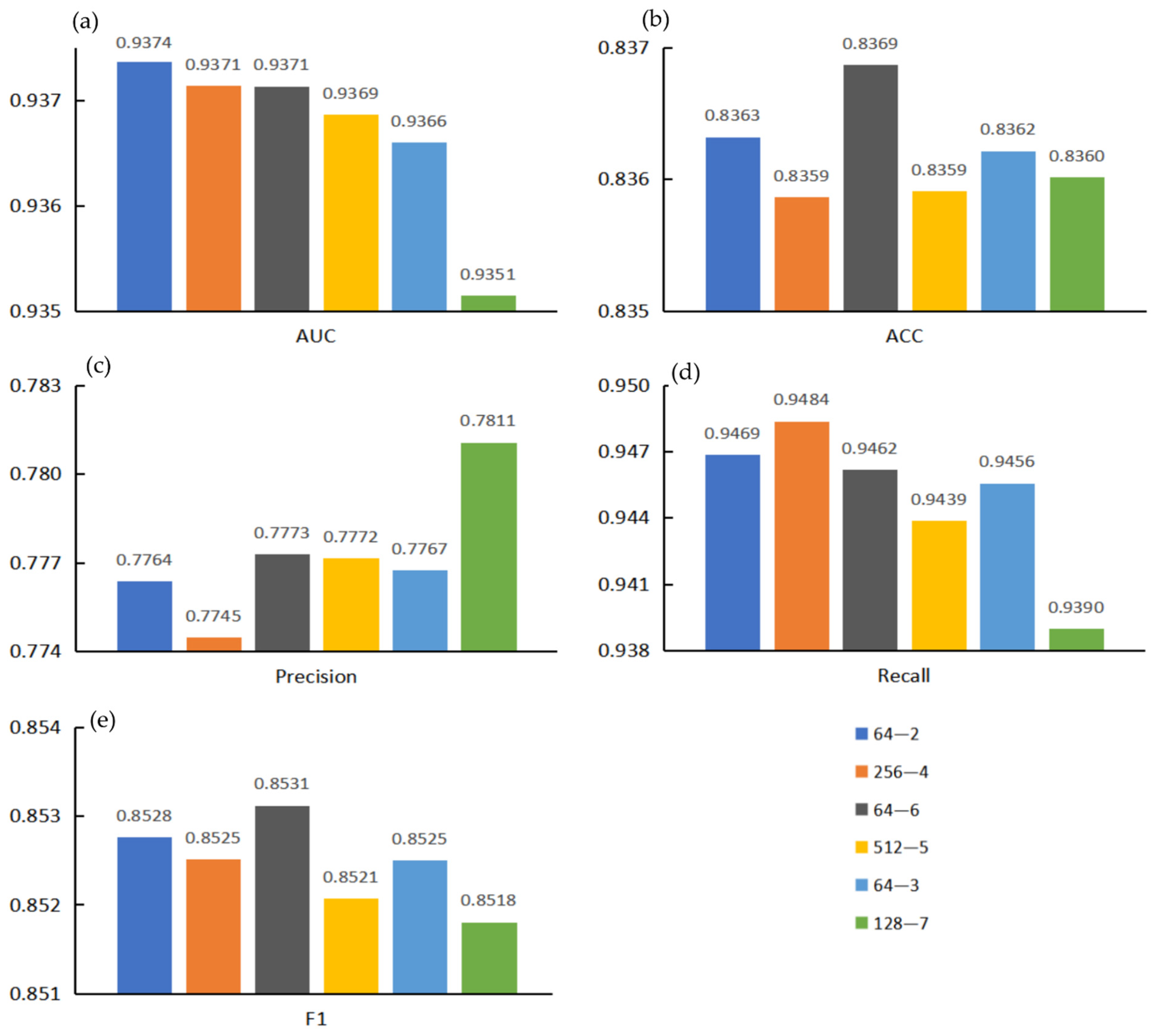
3.3. Effects of Projection Dimension and Encoder Layers on Model Performance

Here, we used the model based on CKSNAP features and the Pearson similarity calculation method to study the influence of projection dimension and encoder layers on prediction performance, changing the number of projection dimensions and encoder layers to obtain the scores of different models on five evaluation indicators. Different projection dimensions will affect the expression ability of nodes. Changing the number of encoder layers can adjust the learning degree of neural networks to node feature information. As can be seen from Figure 5a, with an increase in projection dimensions, the recall rate of the model fluctuated greatly, and the change in F1 score was not obvious. The accuracy score increased significantly with the increase of projection dimensions but dropped sharply when the projection dimension, E, was greater than 256. According to Figure 5b, with an increase in encoder layers, the evaluation indexes of the model showed a downward trend as a whole; especially after L > 6, the indexes of the model declined sharply.

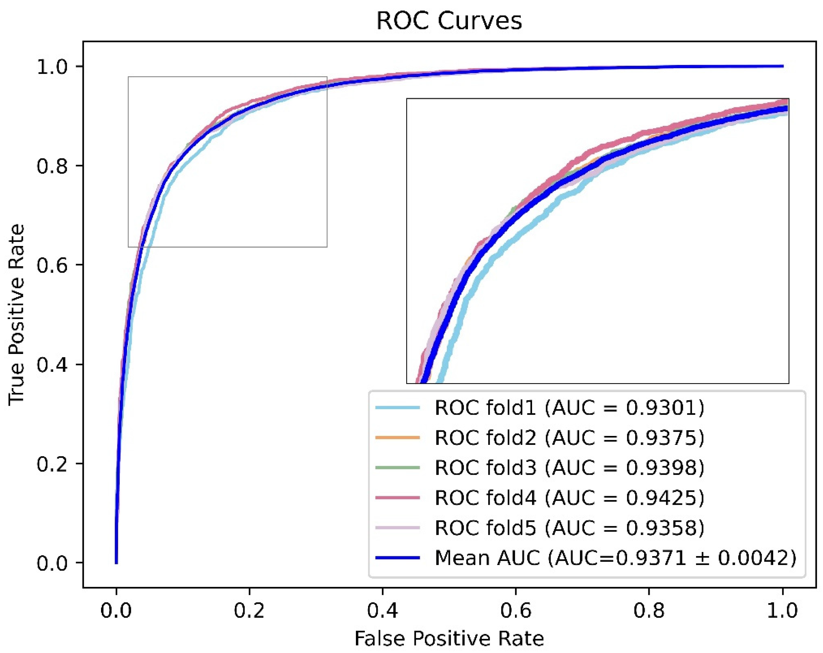
3.4. Performance Evaluation and Comparative Analysis of Related Models

Here, we marked the top five models in each evaluation indicator and screened out the models with two or more markers to obtain the results shown in Figure 6. Considering that Acc was greatly affected by the proportion of positive samples in the sample set, Acc was not taken as the primary evaluation indicator. Precision and recall provide a single view of the performance, whereas F1 score provides a more comprehensive view of the performance and therefore was used for model evaluation. Therefore, considering AUC and F1 score, we noted that the model with project dimensions E = 64 and encoder layer L = 6 had better performance in all aspects. The receiver operating characteristic curve for the 5-fold cross validation experiment is shown in Figure 7. At the same time, the ROC curve of each fold can be seen in Figure S1.
In order to further evaluate the performance of this model, we compared it with six related models (PBMDA [36], LLCMDA [37], EDTMDA [38], GBDTLR [20], MCLPMDA [39], GAEMDA [40]) for comprehensive evaluation. Considering that different studies used different evaluation indicators, only the AUC value that could comprehensively evaluate the performance of the model was selected for comparative analysis. Our study selected the optimal AUC recorded in each paper for comparison, as shown in Table 1. Among the seven models, our model obtained the highest AUC value, which was 0.15% higher than the AUC value of the model with the second highest, GAEMDA.

3.5. Case Studies

In recent years, more and more research has shown that the mutation or abnormal expression of miRNA causes many human diseases [41,42]. In order to further evaluate the performance of our prediction algorithm, three neoplasm diseases were selected for independent case studies—lung neoplasm, esophageal neoplasm, and kidney neoplasm—as it done in the reported method using the same dataset. We deleted the specific diseases of the case study from the training samples to remove bias from the experiments. We used the remaining miRNAs and diseases to construct test samples and ranked them according to the prediction scores. We compared the top 50 prediction results with the dbDEMC databases to obtain the prediction results.
Lung neoplasm is a malignant neoplasm disease occurring in lung parenchyma and stroma [43]. Lung cancer is one of the diseases with the fastest growth rate of morbidity and mortality. It has become the most common cause of death in malignant tumors; the prediction results of our model for miRNA related to lung neoplasm are shown in Table 2. It can be seen that 47 of the top 50 miRNAs could be verified in the dbDEMC database. Esophageal neoplasm is a malignant neoplasm disease that occurs in esophageal epithelial tissue [44,45,46]. Approximately 300,000 people die of esophageal cancer every year in the world. China is one of the high incidence areas of esophageal cancer in the world; the prediction results of our model for miRNA related to esophageal neoplasm are shown in Table 3. It can be seen that 47 of the top 50 miRNAs could be verified in the dbDEMC database. Kidney neoplasm is a common neoplasm disease in the urinary system. The pathological structure of kidney neoplasm is complex, and the cause of disease is variable [47]. Finding a new entry point for diagnosis is of great significance for the timely targeting of patients. The prediction results of our model are shown in Table 4. It can be seen that 37 of the top 50 miRNAs could be verified in the dbDEMC database.

4. Conclusions

In the present study, we used a variety of miRNA sequence features to better retain the sequence similarity information between miRNAs and used a disease–miRNA bipartite graph to mine for potential deeper association information between miRNAs and diseases. Under a 5-fold cross validation, the experimental results showed that the prediction performance of the prediction algorithm based on combined features was not as good as that based on single features, and there was a dependency between the prediction score based on combined features and the prediction model based on corresponding single features. We used this model for case study verification, and the prediction results of three specific tumors also achieved a good hit rate. Therefore, our research is helpful for researchers to quickly and effectively study the relationship between miRNAs and diseases and plays a guiding role in research. It can save time and the cost of wet experiments to find disease-relevant miRNAs. This method can be used to predict the miRNA associated with a disease, and then perform wet experiment verification. Alternatively, there are results from wet experiments, and the method could be used to provide a confidence to refer to in experimental results. However, the analysis and discussion described in this paper is only a small part of the research on the correlation between miRNAs and disease, and there are more questions to be explored. For example, it could be useful to embed more biological information in the structural association between disease and miRNA. For example, when calculating the sequence similarity of miRNAs, we can consider introducing the functional similarity of miRNAs, the MISIM network, and the correlation information between miRNAs and proteins. Further work can focus on finding methods that can obtain deep-seated network structure information without affecting the prediction performance of the model. Finally, considering that the regulatory mechanisms of miRNA in many complex diseases also play an important role in miRNA–disease associations, the analysis of model performance combined with physiological influencing factors is expected to improve future experiments.

Supplementary Materials

The following supporting information can be downloaded at: https://www.mdpi.com/article/10.3390/genes13101759/s1, Figure S1. Receiver operating characteristic curve for each fold experiment. The source code can be downloaded from http://public.aibiochem.net/DNA_RNA/Genes_Human-miRNA-disease-Associations/code.zip (accessed on 1 January 2022).

Author Contributions

Conceptualization, Z.L.; methodology, Z.L.; software, Z.L. and Y.F.; writing—original draft preparation, Y.F. and M.L.; writing—review and editing, Y.F., Y.Z., and M.L.; supervision, Z.L.; funding acquisition, Z.L. All authors have read and agreed to the published version of the manuscript.

Funding

This research was funded by National Natural Science Foundation of China (nos. 62001090) and Fundamental Research Funds for the Central Universities of Sichuan University (nos. YJ2021104).

Institutional Review Board Statement

Not applicable.

Informed Consent Statement

Not applicable.

Data Availability Statement

Not applicable.

Conflicts of Interest

The authors declare no conflict of interest.

References

  1. Crick, F.H.C.; Barnett, L.; Brenner, S.; Watts-Tobin, R.J. General Nature of the Genetic Code for Proteins. Nature 1961, 192, 1227–1232. [Google Scholar] [CrossRef] [PubMed]
  2. Yanofsky, C. Establishing the Triplet Nature of the Genetic Code. Cell 2007, 128, 815–818. [Google Scholar] [CrossRef] [PubMed]
  3. Bertone, P.; Stolc, V.; Royce, T.E.; Rozowsky, J.S.; Urban, A.E.; Zhu, X.; Rinn, J.L.; Tongprasit, W.; Samanta, M.; Weissman, S. Global identification of human transcribed sequences with genome tiling arrays. Science 2004, 306, 2242–2246. [Google Scholar] [CrossRef] [PubMed]
  4. Mishra, R.; Bhattacharya, S.; Rawat, B.S.; Kumar, A.; Kumar, A.; Niraj, K.; Chande, A.; Gandhi, P.; Khetan, D.; Aggarwal, A. MicroRNA-30e-5p has an integrated role in the regulation of the innate immune response during virus infection and systemic lupus erythematosus. iScience 2020, 23, 101322. [Google Scholar] [CrossRef]
  5. Tang, W.; Wan, S.; Yang, Z.; Teschendorff, A.E.; Zou, Q. Tumor Origin Detection with Tissue-Specific miRNA and DNA methylation Markers. Bioinformatics 2018, 34, 398–406. [Google Scholar] [CrossRef] [PubMed]
  6. Wong, L.; You, Z.-H.; Guo, Z.-H.; Yi, H.-C.; Chen, Z.-H.; Cao, M.-Y. MIPDH: A Novel Computational Model for Predicting microRNA–mRNA Interactions by DeepWalk on a Heterogeneous Network. ACS Omega 2020, 5, 17022–17032. [Google Scholar] [CrossRef]
  7. Freeman, W.; Walker, S.; Vrana, K. Quantitative RT-PCR: Pitfalls and potential. BioTechniques 1999, 26, 112–122; 124–125. [Google Scholar] [CrossRef]
  8. Várallyay, É.; Burgyán, J.; Havelda, Z. MicroRNA detection by northern blotting using locked nucleic acid probes. Nat. Protoc. 2008, 3, 190–196. [Google Scholar] [CrossRef]
  9. Baskerville, S.; Bartel, D.P. Microarray profiling of microRNAs reveals frequent coexpression with neighboring miRNAs and host genes. Rna 2005, 11, 241–247. [Google Scholar] [CrossRef]
  10. Zeng, X.; Zhang, X.; Zou, Q. Integrative approaches for predicting microRNA function and prioritizing disease-related microRNA using biological interaction networks. Brief. Bioinform. 2016, 17, 193–203. [Google Scholar] [CrossRef] [Green Version]
  11. Chen, X.; Xie, D.; Zhao, Q.; You, Z.H. MicroRNAs and complex diseases: From experimental results to computational models. Brief. Bioinform. 2019, 20, 515–539. [Google Scholar] [CrossRef] [PubMed]
  12. Jiang, Q.; Hao, Y.; Wang, G.; Juan, L.; Zhang, T.; Teng, M.; Liu, Y.; Wang, Y. Prioritization of disease microRNAs through a human phenome-microRNAome network. BMC Syst. Biol. 2010, 4 (Suppl. S1), S2. [Google Scholar] [CrossRef] [PubMed]
  13. Liu, Y.; Zeng, X.; He, Z.; Zou, Q. Inferring microRNA-disease associations by random walk on a heterogeneous network with multiple data sources. IEEE ACM Trans. Comput. Biol. Bioinform. 2017, 14, 905–915. [Google Scholar] [CrossRef] [PubMed]
  14. Zeng, X.; Liu, L.; Lu, L.; Zou, Q. Prediction of potential disease-associated microRNAs using structural perturbation method. Bioinformatics 2018, 34, 2425–2432. [Google Scholar] [CrossRef]
  15. Zhang, W.; Li, Z.; Guo, W.; Yang, W.; Huang, F. A fast linear neighborhood similarity-based network link inference method to predict microRNA-disease associations. IEEE ACM Trans. Comput. Biol. Bioinform. 2019, 18, 405–415. [Google Scholar] [CrossRef]
  16. Mørk, S.; Pletscher-Frankild, S.; Palleja Caro, A.; Gorodkin, J.; Jensen, L.J. Protein-driven inference of miRNA–disease associations. Bioinformatics 2013, 30, 392–397. [Google Scholar] [CrossRef]
  17. Wang, D.; Wang, J.; Lu, M.; Song, F.; Cui, Q. Inferring the human microRNA functional similarity and functional network based on microRNA-associated diseases. Bioinformatics 2010, 26, 1644–1650. [Google Scholar] [CrossRef]
  18. Chen, X.; Wang, C.C.; Yin, J.; You, Z.H. Novel Human miRNA-Disease Association Inference Based on Random Forest. Mol. Ther. Nucleic Acids 2018, 13, 568–579. [Google Scholar] [CrossRef]
  19. Zeng, X.; Wang, W.; Deng, G.; Bing, J.; Zou, Q. Prediction of potential disease-associated microRNAs by using neural network. Mol. Ther. Nucleic Acids 2019, 16, 566–575. [Google Scholar] [CrossRef]
  20. Zhou, S.; Wang, S.; Wu, Q.; Azim, R.; Li, W. Predicting potential miRNA-disease associations by combining gradient boosting decision tree with logistic regression. Comput. Biol. Chem. 2020, 85, 107200. [Google Scholar] [CrossRef]
  21. Ma, Y.; He, T.; Ge, L.; Zhang, C.; Jiang, X. MiRNA-disease interaction prediction based on kernel neighborhood similarity and multi-network bidirectional propagation. BMC Med. Genom. 2019, 12, 185. [Google Scholar] [CrossRef] [PubMed]
  22. Ping, X.; Ke, H.; Guo, M.; Guo, Y.; Li, J.; Jian, D.; Yong, L.; Dai, Q.; Jin, L.; Teng, Z. Correction: Prediction of microRNAs Associated with Human Diseases Based on Weighted k Most Similar Neighbors. PLoS ONE 2013, 8, 3752034. [Google Scholar] [CrossRef]
  23. Lu, X.; Gao, Y.; Zhu, Z.; Ding, L.; Wang, X.; Liu, F.; Li, J. A Constrained Probabilistic Matrix Decomposition Method for Predicting miRNA-disease Associations. Curr. Bioinform. 2021, 16, 524–533. [Google Scholar] [CrossRef]
  24. Tian, L.; Wang, S.-L. Exploring miRNA Sponge Networks of Breast Cancer by Combining miRNA-disease-lncRNA and miRNA-target Networks. Curr. Bioinform. 2021, 16, 385–394. [Google Scholar] [CrossRef]
  25. Zhang, J.; Sun, Q.; Liang, C. Prediction of lncRNA-disease Associations Based on Robust Multi-label Learning. Curr. Bioinform. 2021, 16, 1179–1189. [Google Scholar] [CrossRef]
  26. Zhang, Y.; Duan, G.; Yan, C.; Yi, H.; Wu, F.-X.; Wang, J. MDAPlatform: A Component-based Platform for Constructing and Assessing miRNA-disease Association Prediction Methods. Curr. Bioinform. 2021, 16, 710–721. [Google Scholar] [CrossRef]
  27. Zhu, Q.; Fan, Y.; Pan, X. Fusing Multiple Biological Networks to Effectively Predict miRNA-disease Associations. Curr. Bioinform. 2021, 16, 371–384. [Google Scholar] [CrossRef]
  28. Jiang, L.; Zhu, J. Review of MiRNA-disease association prediction. Curr. Protein Pept. Sci. 2020, 21, 1044–1053. [Google Scholar] [CrossRef]
  29. Chen, X.; Yan, C.C.; Zhang, X.; You, Z.-H.; Deng, L.; Liu, Y.; Zhang, Y.; Dai, Q. WBSMDA: Within and between score for MiRNA-disease association prediction. Sci. Rep. 2016, 6, 21106. [Google Scholar] [CrossRef]
  30. Yao, D.; Zhan, X.; Kwoh, C.-K. An improved random forest-based computational model for predicting novel miRNA-disease associations. BMC Bioinform. 2019, 20, 624. [Google Scholar] [CrossRef]
  31. Ji, B.-Y.; You, Z.-H.; Cheng, L.; Zhou, J.-R.; Alghazzawi, D.; Li, L.-P. Predicting miRNA-disease association from heterogeneous information network with GraRep embedding model. Sci. Rep. 2020, 10, 6658. [Google Scholar] [CrossRef] [PubMed]
  32. Ji, B.-Y.; You, Z.-H.; Wang, Y.; Li, Z.-W.; Wong, L. DANE-MDA: Predicting microRNA-disease associations via deep attributed network embedding. iScience 2021, 24, 102455. [Google Scholar] [CrossRef]
  33. Yang, Z.; Ren, F.; Liu, C.; He, S.; Sun, G.; Gao, Q.; Yao, L.; Zhang, Y.; Miao, R.; Cao, Y.; et al. dbDEMC: A database of differentially expressed miRNAs in human cancers. BMC Genom. 2010, 11, S5. [Google Scholar] [CrossRef] [PubMed]
  34. Huang, Z.; Shi, J.; Gao, Y.; Cui, C.; Zhang, S.; Li, J.; Zhou, Y.; Cui, Q. HMDD v3.0: A database for experimentally supported human microRNA–disease associations. Nucleic Acids Res. 2018, 47, D1013–D1017. [Google Scholar] [CrossRef] [PubMed]
  35. Chen, X.; Clarence Yan, C.; Luo, C.; Ji, W.; Zhang, Y.; Dai, Q. Constructing lncRNA functional similarity network based on lncRNA-disease associations and disease semantic similarity. Sci. Rep. 2015, 5, 11338. [Google Scholar] [CrossRef] [PubMed]
  36. You, Z.-H.; Huang, Z.-A.; Zhu, Z.; Yan, G.-Y.; Li, Z.-W.; Wen, Z.; Chen, X. PBMDA: A novel and effective path-based computational model for miRNA-disease association prediction. PLoS Comput. Biol. 2017, 13, 1005455. [Google Scholar] [CrossRef] [PubMed]
  37. Qu, Y.; Zhang, H.; Lyu, C.; Liang, C. LLCMDA: A Novel Method for Predicting miRNA Gene and Disease Relationship Based on Locality-Constrained Linear Coding. Front. Genet. 2018, 9, 576. [Google Scholar] [CrossRef] [PubMed]
  38. Chen, X.; Zhu, C.-C.; Yin, J. Ensemble of decision tree reveals potential miRNA-disease associations. PLoS Comput. Biol. 2019, 15, 1007209. [Google Scholar] [CrossRef]
  39. Yu, S.P.; Liang, C.; Xiao, Q.; Li, G.H.; Ding, P.J.; Luo, J.W. MCLPMDA: A novel method for mi RNA-disease association prediction based on matrix completion and label propagation. J. Cell. Mol. Med. 2019, 23, 1427–1438. [Google Scholar] [CrossRef]
  40. Li, Z.; Li, J.; Nie, R.; You, Z.-H.; Bao, W. A graph auto-encoder model for miRNA-disease associations prediction. Brief. Bioinform. 2020, 22, bbaa240. [Google Scholar] [CrossRef]
  41. Birks, D.K.; Barton, V.N.; Donson, A.M.; Handler, M.H.; Vibhakar, R.; Foreman, N.K. Survey of MicroRNA expression in pediatric brain tumors. Pediatr. Blood Cancer 2011, 56, 211–216. [Google Scholar] [CrossRef] [PubMed]
  42. Alder, H.; Taccioli, C.; Chen, H.; Jiang, Y.; Smalley, K.J.; Fadda, P.; Ozer, H.G.; Huebner, K.; Farber, J.L.; Croce, C.M.; et al. Dysregulation of miR-31 and miR-21 induced by zinc deficiency promotes esophageal cancer. Carcinogenesis 2012, 33, 1736–1744. [Google Scholar] [CrossRef] [PubMed]
  43. Torre, L.A.; Siegel, R.L.; Jemal, A. Lung Cancer Statistics. Adv. Exp. Med. Biol. 2016, 893, 1–19. [Google Scholar] [CrossRef]
  44. Linehan, W.M. Genetic basis of kidney cancer: Role of genomics for the development of disease-based therapeutics. Genome Res. 2012, 22, 2089–2100. [Google Scholar] [CrossRef]
  45. Senanayake, U.; Das, S.; Vesely, P.; Alzoughbi, W.; Fröhlich, L.F.; Chowdhury, P.; Leuschner, I.; Hoefler, G.; Guertl, B. miR-192, miR-194, miR-215, miR-200c and miR-141 are downregulated and their common target ACVR2B is strongly expressed in renal childhood neoplasms. Carcinogenesis 2012, 33, 1014–1021. [Google Scholar] [CrossRef] [PubMed]
  46. Zaman, M.S.; Shahryari, V.; Deng, G.; Thamminana, S.; Saini, S.; Majid, S.; Chang, I.; Hirata, H.; Ueno, K.; Yamamura, S. Correction: Up-Regulation of MicroRNA-21 Correlates with Lower Kidney Cancer Survival. PLoS ONE 2012, 7, 31060. [Google Scholar] [CrossRef]
  47. Kim, K.; Taylor, S.L.; Ganti, S.; Guo, L.; Weiss, R.H. Urine Metabolomic Analysis Identifies Potential Biomarkers and Pathogenic Pathways in Kidney Cancer. Omics A J. Integr. Biol. 2011, 15, 293–303. [Google Scholar] [CrossRef] [Green Version]
Figure 1. Technical route of miRNA disease correlation prediction model.
Genes 13 01759 g001
Figure 2. AUC of models based on different features and different similarity calculation methods.
Genes 13 01759 g002
Figure 3. Performance comparison diagram of combined feature-based models and single feature-based models.
Genes 13 01759 g003
Figure 4. Example diagram of dependence of dual feature models on single feature models. (a) is a comparison between the Pearson correlation coefficient model based on Moran feature (blue), the Pearson correlation coefficient model based on CKSNAP feature (dark orange) and the Pearson correlation coefficient model based on Moran+CKSNAP combined feature (gray). (b) is a comparison between the Euclidean distance model based on Moran feature (blue), the Euclidean distance model based on Geary feature (dark orange) and the Euclidean distance model based on Moran+Geary combined feature (gray). (c) is a comparison between the Euclidean distance model based on Geary feature (blue), the Euclidean distance model based on NMBroto feature (dark orange) and the Euclidean distance model based on Geary+NMBroto combined feature (gray). (d) is a comparison between the Pearson correlation coefficient model based on Kmer feature (blue), the Pearson correlation coefficient model based on CKSNAP feature (dark orange) and the Pearson correlation coefficient model based on Kmer+CKSNAP combined feature (gray). (e) is a comparison between the cosine similarity model based on Kmer feature (blue) and the cosine similarity model based on CKSNAP feature (yellow) and the cosine similarity model based on Kmer+CKSNAP combined feature (gray). (f) is a comparison between the Euclidean distance model based on Kmer feature (blue), the Euclidean distance model based on Moran feature (dark orange) and the Euclidean distance model based on Kmer+Moran combined feature (gray).
Genes 13 01759 g004
Figure 5. (a) Effects of different projection dimensions on model performance; (b) influence of different encoder layers on model performance.
Genes 13 01759 g005
Figure 6. The top five evaluation indicators were marked and summarized to obtain two or more models. (a) AUC value comparison; (b) ACC value comparison; (c) Precision value comparison; (d) Recall value comparison; (e) F1 value comparison.
Genes 13 01759 g006
Figure 7. The model with project dimension E = 64 and encoder layers L = 6 had better performance.
Genes 13 01759 g007
Table 1. Comparative analysis of our model and related models.
ModelAUC (%)
PBMDA91.72
LLCMDA91.90
EDTMDA91.92
GBDTLR92.74
MCLPMDA93.20
GAEMDA93.56
Our Model93.71
Table 2. Lung neoplasm associated miRNA Top 50 predicted by hmdd v3.2.
miRNAdbDEMCmiRNAdbDEMC
hsa-mir-586Confirmedhsa-mir-329-5pConfirmed
hsa-mir-208b-5pConfirmedhsa-mir-1264Confirmed
hsa-mir-376b-5pConfirmedhsa-mir-618Confirmed
hsa-mir-3613-5pConfirmedhsa-mir-599Confirmed
hsa-mir-4775Confirmedhsa-mir-517c-3pUnconfirmed
hsa-mir-544aConfirmedhsa-mir-384Confirmed
hsa-mir-450a-5pConfirmedhsa-mir-581Confirmed
hsa-mir-376c-5pConfirmedhsa-mir-578Confirmed
hsa-mir-376a-5pConfirmedhsa-mir-19b-2-5pConfirmed
hsa-mir-190a-5pConfirmedhsa-mir-552-5pConfirmed
hsa-mir-875-5pConfirmedhsa-mir-5590-5pConfirmed
hsa-mir-3682-5pConfirmedhsa-mir-450a-1-3pConfirmed
hsa-mir-302fConfirmedhsa-mir-454-5pConfirmed
hsa-mir-5586-5pConfirmedhsa-mir-942-5pConfirmed
hsa-mir-450b-5pConfirmedhsa-mir-548lConfirmed
hsa-mir-576-5pConfirmedhsa-mir-548kConfirmed
hsa-mir-4295Confirmedhsa-mir-1185-5pConfirmed
hsa-mir-1282Confirmedhsa-mir-548am-5pConfirmed
hsa-mir-5009-5pConfirmedhsa-mir-613Confirmed
hsa-mir-655-5pConfirmedhsa-mir-1248Confirmed
hsa-mir-16-2-3pConfirmedhsa-mir-544bConfirmed
hsa-mir-548d-5pConfirmedhsa-mir-3913-5pConfirmed
hsa-mir-1179Confirmedhsa-mir-548c-5pConfirmed
hsa-mir-876-5pConfirmedhsa-mir-570-5pUnconfirmed
hsa-mir-1206Unconfirmedhsa-mir-651-5pConfirmed
Table 3. Esophageal neoplasm associated miRNA Top 50 predicted by hmdd v3.2.
miRNAdbDEMCmiRNAdbDEMC
hsa-mir-1179Confirmedhsa-mir-450b-5pConfirmed
hsa-mir-1206Confirmedhsa-mir-4775Confirmed
hsa-mir-1264Confirmedhsa-mir-493-5pConfirmed
hsa-mir-1282Confirmedhsa-mir-495-5pConfirmed
hsa-mir-135a-5pConfirmedhsa-mir-5009-5pConfirmed
hsa-mir-136-5pConfirmedhsa-mir-517c-3pConfirmed
hsa-mir-16-2-3pConfirmedhsa-mir-544aConfirmed
hsa-mir-190a-5pConfirmedhsa-mir-545-5pConfirmed
hsa-mir-196a-5pConfirmedhsa-mir-548d-5pConfirmed
hsa-mir-199b-5pConfirmedhsa-mir-552-5pUnconfirmed
hsa-mir-19b-2-5pConfirmedhsa-mir-5586-5pConfirmed
hsa-mir-202-5pConfirmedhsa-mir-5590-5pConfirmed
hsa-mir-208b-5pConfirmedhsa-mir-576-5pConfirmed
hsa-mir-29a-5pConfirmedhsa-mir-578Confirmed
hsa-mir-329-5pUnconfirmedhsa-mir-581Confirmed
hsa-mir-3613-5pConfirmedhsa-mir-586Confirmed
hsa-mir-3682-5pConfirmedhsa-mir-599Confirmed
hsa-mir-376a-2-5pConfirmedhsa-mir-618Confirmed
hsa-mir-376a-5pConfirmedhsa-mir-655-5pConfirmed
hsa-mir-376c-5pConfirmedhsa-mir-7-5pConfirmed
hsa-mir-384Confirmedhsa-mir-875-5pConfirmed
hsa-mir-4295Confirmedhsa-mir-876-5pConfirmed
hsa-mir-4423-5pConfirmedhsa-mir-95-5pConfirmed
hsa-mir-450a-1-3pUnconfirmedhsa-mir-9-5pConfirmed
hsa-mir-450a-5pConfirmedhsa-mir-29b-1-5pConfirmed
Table 4. Kidney neoplasm associated miRNA Top 50 predicted by hmdd v3.2.
miRNAdbDEMCmiRNAdbDEMC
hsa-mir-105-5pConfirmedhsa-mir-449aConfirmed
hsa-mir-1179Confirmedhsa-mir-449c-5pConfirmed
hsa-mir-1204Confirmedhsa-mir-4775Confirmed
hsa-mir-1244Confirmedhsa-mir-4795-5pUnconfirmed
hsa-mir-1264Confirmedhsa-mir-517c-3pConfirmed
hsa-mir-1267Confirmedhsa-mir-5193Unconfirmed
hsa-mir-1282Confirmedhsa-mir-520hUnconfirmed
hsa-mir-1284Confirmedhsa-mir-543Confirmed
hsa-mir-1322Confirmedhsa-mir-548c-5pUnconfirmed
hsa-mir-135b-5pConfirmedhsa-mir-5692bUnconfirmed
hsa-mir-136-5pConfirmedhsa-mir-576-5pConfirmed
hsa-mir-147b-5pUnconfirmedhsa-mir-577Confirmed
hsa-mir-149-5pConfirmedhsa-mir-586Confirmed
hsa-mir-18b-5pConfirmedhsa-mir-606Confirmed
hsa-mir-202-5pConfirmedhsa-mir-616-5pConfirmed
hsa-mir-212-5pConfirmedhsa-mir-626Unconfirmed
hsa-mir-23cConfirmedhsa-mir-633Confirmed
hsa-mir-3120-5pUnconfirmedhsa-mir-644aUnconfirmed
hsa-mir-3149Confirmedhsa-mir-645Confirmed
hsa-mir-32-5pUnconfirmedhsa-mir-764Unconfirmed
hsa-mir-340-5pConfirmedhsa-mir-889-5pUnconfirmed
hsa-mir-3662Confirmedhsa-mir-934Confirmed
hsa-mir-3682-5pUnconfirmedhsa-mir-942-5pConfirmed
hsa-mir-4295Confirmedhsa-mir-943Confirmed
hsa-mir-4443Confirmedhsa-mir-944Confirmed
Publisher’s Note: MDPI stays neutral with regard to jurisdictional claims in published maps and institutional affiliations.

