
Cancer Subtype Recognition Based on Laplacian Rank Constrained Multiview Clustering


Abstract
1. Introduction
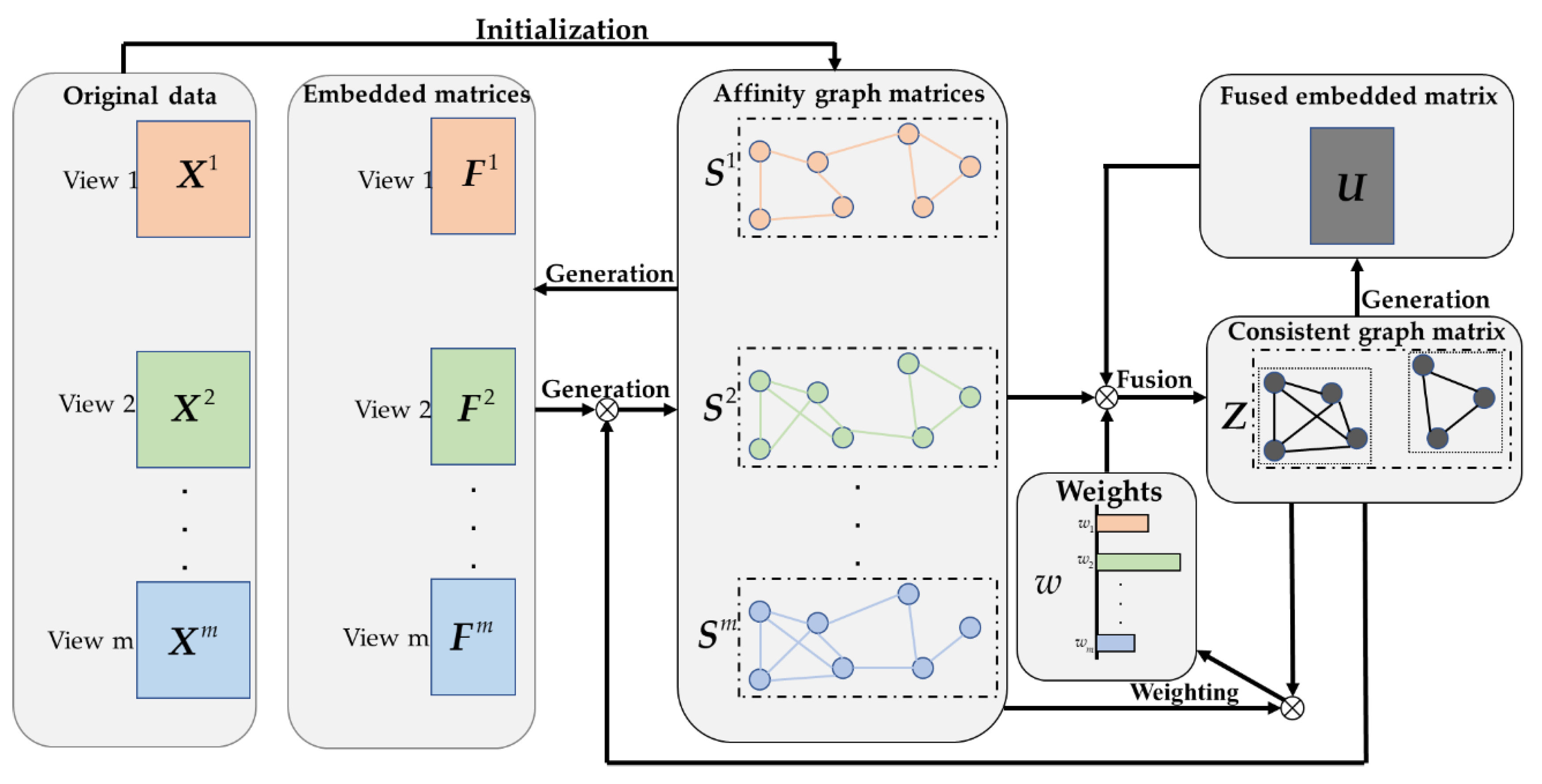
2. Methods
2.1. Construction of Affinity Graph Based on LRC
2.2. Graph Fusion with LRC
2.3. LRCMC Algorithm
- Our method can effectively learn a set of affinity graph matrices with c connected components, instead of most multiview clustering methods requiring predefined graphs;
- In the graph fusion process, we assign the weight to each view to represent their contribution to the consistent graph Z, rather than simply superimposing then together;
- We use LRC to constantly adjust the structures of and Z, and at the same time complete the task of clustering.
2.4. Optimization Algorithm of LRCMC
- 1.
- Fix , , Z and U, solve ;
- 2.
- Fix , , Z and U, solve ;
- 3.
- Fix , , Z and U, solve ;
- 4.
- Fix , , and U, solve Z.;
- 5.
- Fix , , and Z, solve U.
3. Experiments’ Results
3.1. Comparison Experiments on Benchmark Datasets
- 3-source [20]: It contains 169 news that were reported by three news magazines, i.e., BBC, Reuters, and The Guardian. There are six different thematic labels for each news;
- Calt-7 [36]: The object recognition dataset is drawn from the Caltech101 dataset to screen 7 widely used classes, i.e., faces, motorbikes, dollar bill, Garfield, stop sign, and Windsor chair. Each class has 1474 images. Each image is described by 6 features, i.e., GABOR, wavelet moment (WM), CENT, HOG, GIST and LBP;
- MSRC [37]: The scene recognition dataset contains 7 classes of aircraft, car, bicycle, cow, faces, tree, and building. Each image is described by 5 features, i.e., color moment (CMT), HOG, LBP, CENT, GIST;
- WebKB [20]: It collects 203 web pages in 4 classes from the University’s Computer science department. Each page has 3 features, i.e., the content of the page, the anchor text of the hyperlink, and the text description in the title.
| Algorithm 1. LRCMC algorithm |
| Input: Original data with m views, the number of clusters c, the number of neighbors k, the regularization parameter . Output: The learned consensus matrix Z. Initialize the affinity matrices for each view by solving the following problem: ; Initialize the embedded matrices for each view by using Equation (1); Initialize the weights for each view by ; Initialize Z by connecting with ; Initialize the fused embedded matrix U by using Equation (23); Repeat Fix , , Z and U, update by using Equation (19); Fix , , Z and U, update by using Equation (1); Fix , , Z and U, update by using Equation (6); Fix , , and U, update Z by using Equation (22); Fix , , and Z. update U by using Equation (23); Until Satisfy Theorem 1 or the maximum iteration reached. The learned consensus matrix Z with exact c connected components, which are the final clusters. |
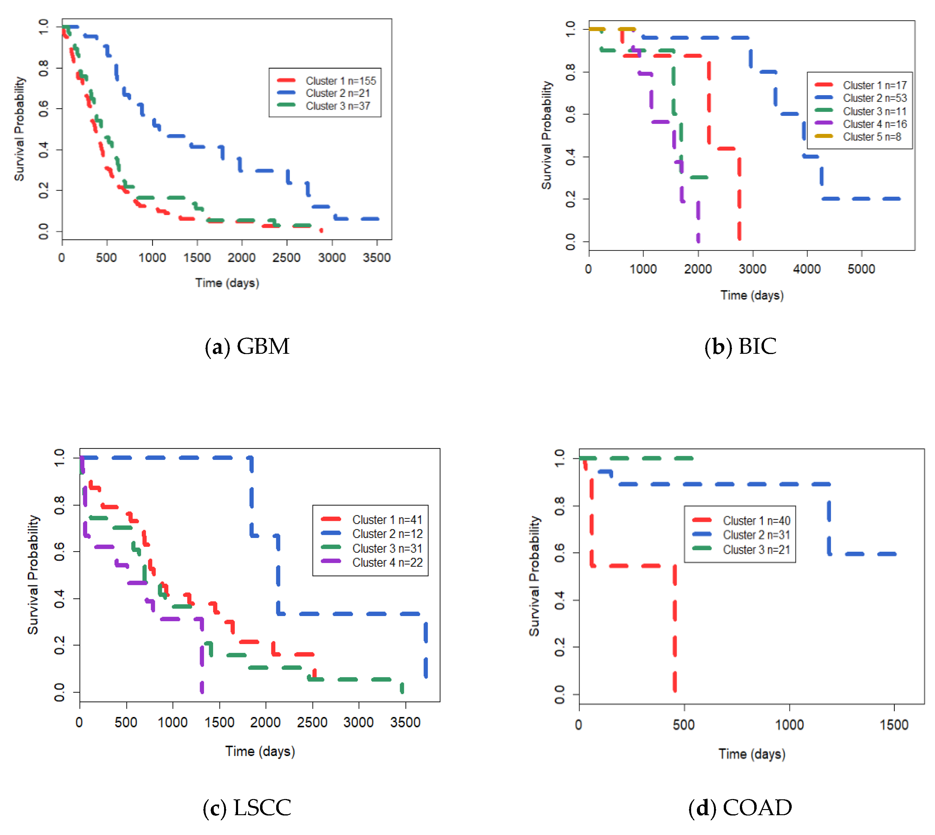
3.2. Comparison Experiments on TCGA Datasets
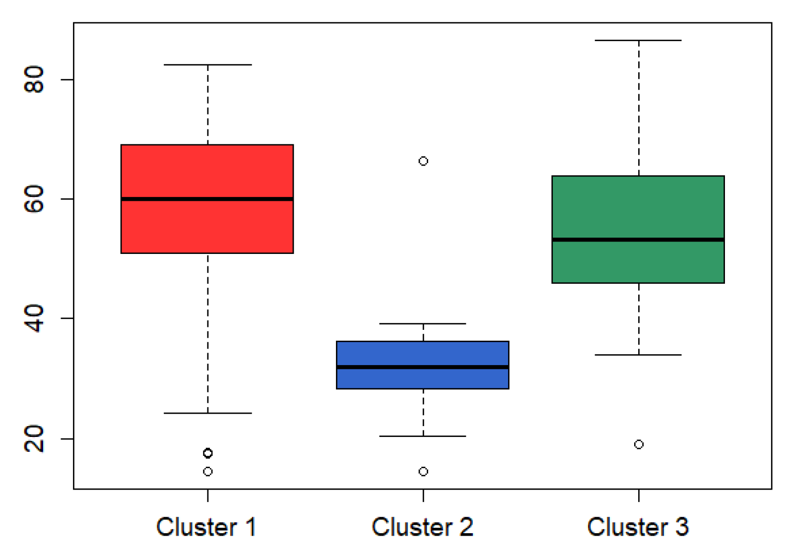
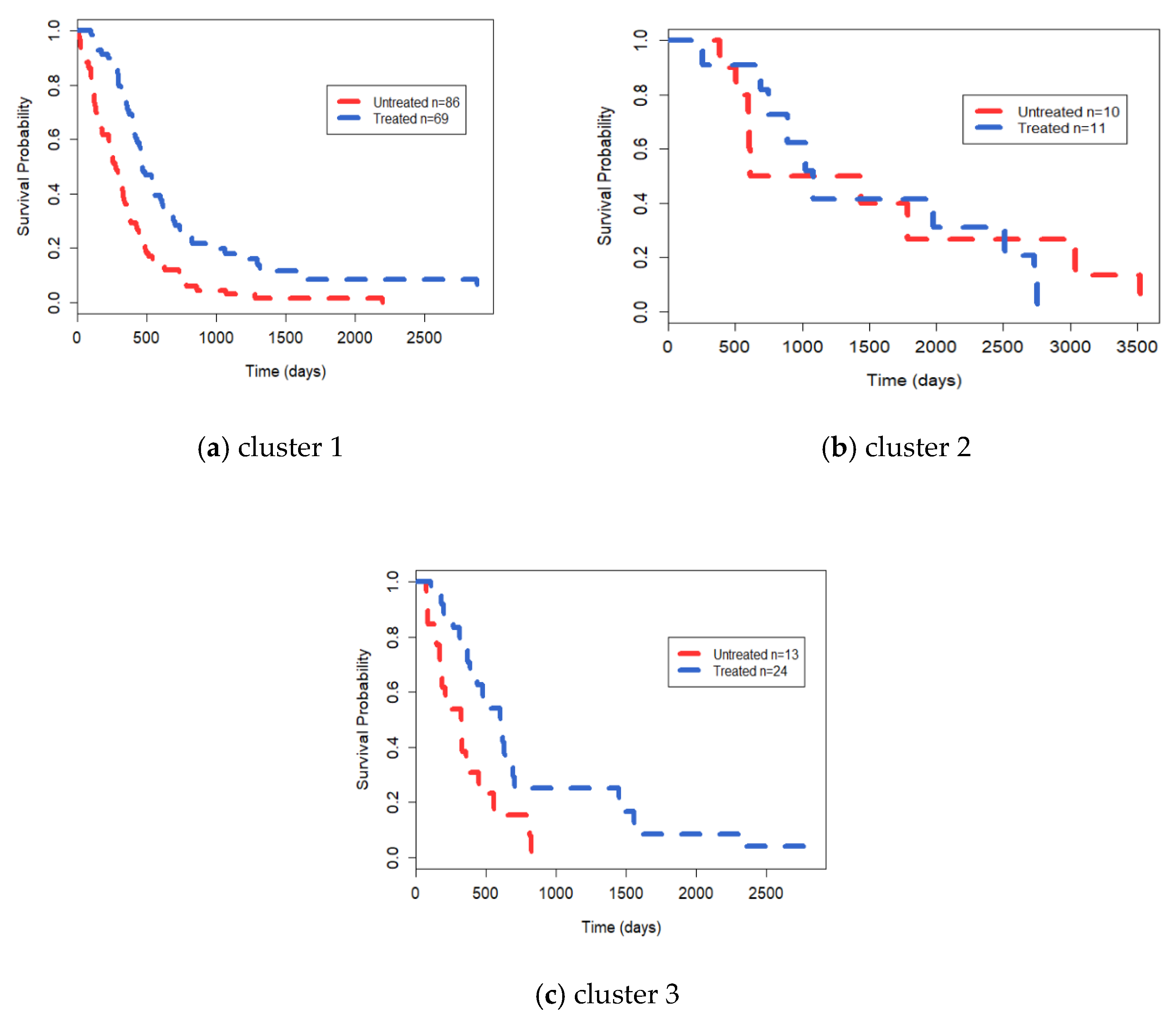
3.3. Analysis on GBM Dataset
4. Discussion and Conclusions
Supplementary Materials
Author Contributions
Funding
Institutional Review Board Statement
Informed Consent Statement
Data Availability Statement
Acknowledgments
Conflicts of Interest
References
- Burrell, R.A.; McGranahan, N.; Bartek, J.; Swanton, C. The causes and consequences of genetic heterogeneity in cancer evolution. Nature 2013, 501, 338–345. [Google Scholar] [CrossRef]
- Bedard, P.L.; Hansen, A.R.; Ratain, M.J.; Siu, L.L. Tumour heterogeneity in the clinic. Nature 2013, 501, 355–364. [Google Scholar] [CrossRef]
- Schuster, S.C. Next-generation sequencing transforms today’s biology. Nat. Methods 2008, 5, 16–18. [Google Scholar] [CrossRef]
- Akbani, R.; Ng, K.S.; Werner, H.M.; Zhang, F.; Ju, Z.; Liu, W.; Liu, W.; Yang, J.Y.; Yoshihara, K.; Li, J.; et al. A pan-cancer proteomic analysis of The Cancer Genome Atlas (TCGA) project. Cancer Res. 2014, 74, 4262. [Google Scholar]
- Shen, R.; Olshen, A.B.; Ladanyi, M. Integrative clustering of multiple genomic data types using a joint latent variable model with application to breast and lung cancer subtype analysis. Bioinformatics 2009, 25, 2906–2912. [Google Scholar] [CrossRef]
- Mo, Q.; Wang, S.; Seshan, V.E.; Olshen, A.B.; Schultz, N.; Sander, C.; Powers, R.S.; Ladanyi, M.; Shen, R. Pattern discovery and cancer gene recognition in integrated cancer genomic data. Proc. Natl. Acad. Sci. USA 2013, 110, 4245–4250. [Google Scholar] [CrossRef]
- Shihua, Z.; Chun-Chi, L.; Wenyuan, L.; Hui, S.; Laird, P.W.; Jasmine, Z.X. Discovery of multi-dimensional modules by integrative analysis of cancer genomic data. Nucleic Acids Res. 2012, 19, 9379–9391. [Google Scholar]
- Wu, D.; Wang, D.; Zhang, M.Q.; Gu, J. Fast dimension reduction and integrative clustering of multi-omics data using low-rank approximation: Application to cancer molecular classification. BMC Genom. 2015, 16, 1022. [Google Scholar] [CrossRef] [PubMed]
- Speicher, N.K.; Pfeifer, N. Integrating different data types by regularized unsupervised multiple kernel learning with application to cancer subtype discovery. Bioinformatics 2015, 31, i268–i275. [Google Scholar] [CrossRef] [PubMed]
- Shi, Q.; Zhang, C.; Peng, M.; Yu, X.; Zeng, T.; Liu, J.; Chen, L. Pattern fusion analysis by adaptive alignment of multiple heterogeneous omics data. Bioinformatics 2017, 33, 2706–2714. [Google Scholar] [CrossRef] [PubMed]
- Wang, B.; Mezlini, A.M.; Demir, F.; Fiume, M.; Tu, Z.; Brudno, M.; Haibe-Kains, B.; Goldenberg, A. Similarity network fusion for aggregating data types on a genomic scale. Nat. Methods 2014, 11, 333. [Google Scholar] [CrossRef] [PubMed]
- Ma, T.; Zhang, A. Integrate multi-omic data using affinity network fusion (anf) for cancer patient clustering. In Proceedings of the IEEE International Conference on Bioinformatics and Biomedicine (BIBM), Kansas City, MO, USA, 13–16 November 2017; pp. 398–403. [Google Scholar]
- Guo, Y.; Zheng, J.; Shang, X.; Li, Z. A similarity regression fusion model for integrating multi-omics data to identify cancer subtypes. Genes 2018, 9, 314. [Google Scholar] [CrossRef] [PubMed]
- Guo, Y.; Li, H.; Cai, M.; Li, L. Integrative subspace clustering by common and specific decomposition for applications on cancer subtype recognition. BMC Med Genom. 2019, 12, 1–17. [Google Scholar] [CrossRef]
- Meng, C.; Helm, D.; Frejno, M.; Kuster, B. moCluster: Identifying joint patterns across multiple omics data sets. J. Proteome Res. 2016, 15, 755–765. [Google Scholar] [CrossRef]
- Shi, Q.; Hu, B.; Zeng, T.; Zhang, C. Multi-view subspace clustering analysis for aggregating multiple heterogeneous omics data. Front. Genet. 2019, 10, 744. [Google Scholar] [CrossRef] [PubMed]
- Yu, Y.; Zhang, L.H.; Zhang, S. Simultaneous clustering of multiview biomedical data using manifold optimization. Bioinformatics 2019, 35, 4029–4037. [Google Scholar] [CrossRef]
- Kumar, A.; Daumé, H. A co-training approach for multi-view spectral clustering. In Proceedings of the 28th international conference on machine learning (ICML-11), Bellevue, WA, USA, 28 June –2 July 2011; pp. 393–400. [Google Scholar]
- Hu, Z.; Nie, F.; Chang, W.; Hao, S.; Wang, R.; Li, X. Multi-view spectral clustering via sparse graph learning. Neurocomputing 2020, 384, 1–10. [Google Scholar] [CrossRef]
- Wang, H.; Yang, Y.; Liu, B. GMC: Graph-based multi-view clustering. IEEE Trans. Knowl. Data Eng. 2019, 32, 1116–1129. [Google Scholar] [CrossRef]
- Zhan, K.; Zhang, C.; Guan, J.; Wang, J. Graph learning for multiview clustering. IEEE Trans. Cybern. 2017, 48, 2887–2895. [Google Scholar] [CrossRef]
- Liu, B.Y.; Huang, L.; Wang, C.D.; Lai, J.H.; Yu, P. Multi-view Consensus Proximity Learning for Clustering. IEEE Trans. Knowl. Data Eng. 2020. [Google Scholar] [CrossRef]
- Nie, F.; Cai, G.; Li, X. Multi-view clustering and semi-supervised classification with adaptive neighbours. Proc. AAAI Conf. Artif. Intell. 2017, 31, 2408–2414. [Google Scholar]
- Nie, F.; Li, J.; Li, X. Self-weighted Multiview Clustering with Multiple Graphs. IJCAI 2017, 2564–2570. [Google Scholar] [CrossRef]
- Wang, Y.; Zhang, W.; Wu, L.; Lin, X.; Fang, M.; Pan, S. Iterative views agreement: An iterative low-rank based structured optimization method to multi-view spectral clustering. arXiv 2016, arXiv:1608.05560. [Google Scholar]
- Cao, X.; Zhang, C.; Fu, H.; Liu, S.; Zhang, H. Diversity-induced multi-view subspace clustering. In Proceedings of the IEEE Conference on Computer Vision and Pattern Recognition, Boston, MA, USA, 7–12 June 2015; pp. 586–594. [Google Scholar]
- Nie, F.; Wang, X.; Jordan, M.; Huang, H. The constrained laplacian rank algorithm for graph-based clustering. Proc. AAAI Conf. Artif. Intell. 2016, 30, 1969–1976. [Google Scholar]
- Hu, H.; Lin, Z.; Feng, J.; Zhou, J. Smooth representation clustering. In Proceedings of the IEEE Conference on Computer Vision and Pattern Recognition, Columbus, OH, USA, 23–28 June 2014; pp. 3834–3841. [Google Scholar]
- Kang, Z.; Peng, C.; Cheng, Q. Twin learning for similarity and clustering: A unified kernel approach. In Proceedings of the AAAI Conference on Artificial Intelligence, San Francisco, CA, USA, 4–9 February 2017. [Google Scholar]
- Mohar, B.; Alavi, Y.; Chartrand, G.; Oellermann, O.R. The Laplacian spectrum of graphs. Graph. Theory Comb. Appl. 1991, 2, 871–898. [Google Scholar]
- Chung, F.R.; Graham, F.C. Spectral Graph Theory; American Mathematical Society: Providence, RI, USA, 1997. [Google Scholar]
- Tarjan, R. Depth-first search and linear graph algorithms. SIAM J. Comput. 1972, 1, 146–160. [Google Scholar] [CrossRef]
- Fan, K. On a theorem of Weyl concerning eigenvalues of linear transformations I. Proc. Natl. Acad. Sci. USA 1949, 35, 652. [Google Scholar] [CrossRef]
- Boyd, S.; Boyd, S.P.; Vandenberghe, L. Convex Optimization; Cambridge University Press: London, UK, 2004. [Google Scholar]
- Wright, J.; Yang, A.Y.; Ganesh, A.; Sastry, S.S.; Ma, Y. Robust face recognition via sparse representation. IEEE Trans. Pattern Anal. Mach. Intell. 2008, 31, 210–227. [Google Scholar] [CrossRef]
- Dueck, D.; Frey, B.J. Non-metric affinity propagation for unsupervised image categorization. In Proceedings of the 2007 IEEE 11th International Conference on Computer Vision, Rio de Janeiro, Brazil, 14–21 October 2007; pp. 1–8. [Google Scholar]
- Winn, J.; Jojic, N. Locus: Learning object classes with unsupervised segmentation. Tenth IEEE Int. Conf. Comput. Vis. 2005, 1, 756–763. [Google Scholar]
- Hosmer, D.W.; Lemeshow, S.; May, S. Applied survival analysis: Regression modeling of time to event data. J. Stat. Plan. Inference 2000, 91, 173–175. [Google Scholar]
- Verhaak, R.G.; Hoadley, K.A.; Purdom, E.; Wang, V.; Qi, Y.; Wilkerson, M.D.; Miller, C.R.; Ding, L.; Golub, T.; Mesirov, J.P.; et al. Integrated genomic analysis identifies clinically relevant subtypes of glioblastoma characterized by abnormalities in PDGFRA, IDH1, EGFR, and NF1. Cancer Cell 2010, 17, 98–110. [Google Scholar] [CrossRef] [PubMed]
- Noushmehr, H.; Weisenberger, D.J.; Diefes, K.; Phillips, H.S.; Pujara, K.; Berman, B.P.; Pan, F.; Pelloski, C.E.; Sulman, E.P.; Bhat, K.P.; et al. Recognition of a CpG island methylator phenotype that defines a distinct subgroup of glioma. Cancer Cell 2010, 17, 510–522. [Google Scholar] [CrossRef]
- Brennan, C.W.; Verhaak, R.G.; McKenna, A.; Campos, B.; Noushmehr, H.; Salama, S.R.; Zheng, S.; Chakravarty, D.; Sanborn, Z.; Berman, S.H.; et al. The somatic genomic landscape glioblastoma. Cell 2013, 155, 462–477. [Google Scholar] [CrossRef] [PubMed]
- Lee, D.H.; Lee, T.H.; Jung, C.H.; Kim, Y.H. Wogonin induces apoptosis by activating the AMPK and p53 signaling pathways in human glioblastoma cells. Cell. Signal. 2012, 24, 2216–2225. [Google Scholar] [CrossRef] [PubMed]
- Rodriguez, A.; Brown, C.; Badie, B. Chimeric antigen receptor T-cell therapy for glioblastoma. Transl. Res. 2017, 187, 93–102. [Google Scholar] [CrossRef]
- Villano, J.L.; Collins, C.A.; Manasanch, E.E.; Ramaprasad, C.; van Besien, K. Aplastic anaemia in patient with glioblastoma multiforme treated with temozolomide. Lancet Oncol. 2006, 7, 436–438. [Google Scholar] [CrossRef]
- Li, Y.; Wu, F.X.; Ngom, A. A review on machine learning principles for multi-view biological data integration. Brief. Bioinform. 2018, 19, 325–340. [Google Scholar] [CrossRef]
- Liang, X.; Zhang, P.; Yan, L.; Fu, Y.; Peng, F.; Qu, L.; Shao, M.; Chen, Y.; Chen, Z. LRSSL: Predict and interpret drug–disease associations based on data integration using sparse subspace learning. Bioinformatics 2017, 33, 1187–1196. [Google Scholar] [CrossRef]
- Bashashati, A.; Haffari, G.; Ding, J.; Ha, G.; Lui, K.; Rosner, J.; Huntsman, D.G.; Caldas, C.; Aparicio, S.A.; Shah, S.P. DriverNet: Uncovering the impact of somatic driver mutations on transcriptional networks in cancer. Genome Biol. 2012, 13, 1–14. [Google Scholar] [CrossRef] [PubMed]
- Ritchie, M.D.; Holzinger, E.R.; Li, R.; Pendergrass, S.A.; Kim, D. Methods of integrating data to uncover genotype–phenotype interactions. Nat. Rev. Genet. 2015, 16, 85–97. [Google Scholar] [CrossRef]


| Dataset | n | m | c | d1 | d2 | d3 | d4 | d5 | d6 |
|---|---|---|---|---|---|---|---|---|---|
| 3-source | 169 | 3 | 6 | 3560 | 3631 | 3638 | - | - | - |
| Calt-7 | 1474 | 6 | 7 | 48 | 40 | 254 | 1984 | 512 | 928 |
| MSRC | 210 | 5 | 7 | 48 | 100 | 256 | 1302 | 512 | - |
| WebKB | 203 | 3 | 4 | 1703 | 230 | 230 | - | - | - |
| Datasets | Methods | ACC | NMI | Purity |
|---|---|---|---|---|
| 3-source | ANF | 0.4970 (0.0000) | 0.2804 (0.0000) | 0.5325 (0.0000) |
| SNF | 0.7811 (0.0000) | 0.6942 (0.0000) | 0.8166 (0.0000) | |
| PFA | 0.4562 (0.0761) | 0.2247 (0.0713) | 0.7160 (0.0578) | |
| MVCMO | 0.4221 (0.0123) | 0.3035 (0.0128) | 0.5266 (0.0118) | |
| LRCMC | 0.8107 (0.0000) | 0.7218 (0.0000) | 0.8462 (0.0000) | |
| Calt-7 | ANF | 0.6696 (0.0000) | 0.6203 (0.0000) | 0.8684 (0.0000) |
| SNF | 0.6601 (0.0000) | 0.5637 (0.0000) | 0.8562 (0.0000) | |
| PFA | - | - | - | |
| MVCMO | 0.6654 (0.0100) | 0.5179 (0.0355) | 0.8464 (0.0083) | |
| LRCMC | 0.8548 (0.0000) | 0.7694 (0.0000) | 0.8921 (0.0000) | |
| MSRC | ANF | 0.8048 (0.0000) | 0.7297 (0.0000) | 0.8143 (0.0000) |
| SNF | 0.8429 (0.0000) | 0.7514 (0.0000) | 0.8429 (0.0000) | |
| PFA | - | - | - | |
| MVSCO | 0.7800 (0.0544) | 0.6711 (0.0628) | 0.7838 (0.0462) | |
| LRCMC | 0.8905 (0.0000) | 0.7922 (0.0000) | 0.8905 (0.0000) | |
| WebKB | ANF | 0.6798 (0.0000) | 0.1718 (0.0000) | 0.6946 (0.0000) |
| SNF | 0.7044 (0.0000) | 0.2407 (0.0000) | 0.7192 (0.0000) | |
| PFA | 0.7143 (0.0000) | 0.3191 (0.0000) | 0.8128 (0.0000) | |
| MVCMO | 0.7652 (0.0346) | 0.3548 (0.0448) | 0.7833 (0.0323) | |
| LRCMC | 0.8079 (0.0000) | 0.5081 (0.0000) | 0.8424 (0.0000) |
| Datasets | N | mRNA Expression | DNA Methylation | miRNA Expression |
|---|---|---|---|---|
| GBM | 213 | 12,042 | 1305 | 534 |
| BIC | 105 | 17,814 | 23,094 | 354 |
| LSCC | 106 | 12,042 | 23,074 | 352 |
| COAD | 92 | 17,814 | 23,088 | 312 |
| Methods | GBM | BIC | LSCC | COAD |
|---|---|---|---|---|
| ANF | 5.8 × 10⁻⁴ | 3.6 × 10⁻⁴ | 8.9 × 10⁻³ | 9.0 × 10⁻³ |
| SNF | 5.0×10⁻⁵ | 6.9×10⁻⁴ | 7.8 × 10⁻³ | 1.6 × 10⁻³ |
| PFA | 1.8×10⁻⁴ | 3.1×10⁻⁴ | 1.1 × 10⁻² | 2.4 × 10⁻² |
| MVCMO | 1.4×10⁻³ | 3.5×10⁻⁴ | 9.1 × 10⁻³ | 8.5 × 10⁻³ |
| LRCMC | 1.3 × 10⁻⁵ | 3.7 × 10⁻⁵ | 3.8 × 10⁻³ | 1.2 × 10⁻³ |
| Our Cluster | mRNA-Expression-Based Subtypes | Methylation-Based Subtypes | ||||
|---|---|---|---|---|---|---|
| Mesenchymal | Classical | Neural | Proneural | G-CLMP | Non-G-CLMP | |
| cluster 1 | 46 | 54 | 27 | 30 | 0 | 155 |
| cluster 2 | 1 | 0 | 1 | 19 | 20 | 1 |
| cluster 3 | 12 | 11 | 7 | 7 | 0 | 37 |
| Our Cluster | CDKN2A.del. | CDKN2B.del. | C9orf53.del. | MTAP.del. | EGFR.ampl. | IDH1 |
|---|---|---|---|---|---|---|
| cluster 1 | 84 (56.4%) | 84 (56.4%) | 80 (53.7%) | 57 (38.3%) | 70 (47.0%) | 0 (0%) |
| cluster 2 | 6 (28.6%) | 6 (28.6%) | 6 (28.6%) | 5 (23.8%) | 0 (0%) | 10 (66.7%) |
| cluster 3 | 24 (68.9%) | 23 (62.2%) | 24 (68.9%) | 21 (56.8%) | 19 (51.4%) | 0 (0%) |
| ENRICHMENT Analysis | Cluster 1 | Cluster 2 | Cluster 3 |
|---|---|---|---|
| GO:BP enriched terms | 1. Epithelial cell differentiation 2. Epithelium development 3. Cell adhesion 4. Biological adhesion 5. cell–cell adhesion | 1. Protein targeting to ER 2. Establishment of protein localization to endoplasmic reticulum 3. Protein localization to endoplasmic reticulum 4. Peptide metabolic process 5. Protein targeting protein targeting | 1. SRP-dependent cotranslational protein targeting to membrane 2. Cotranslational protein targeting to membrane 3. Nuclear-transcribed mRNA catabolic process, nonsense-mediated decay 4. Protein targeting to ER 5. Establishment of protein localization to endoplasmic reticulum |
| KEGG enriched pathway terms | 1. Cell adhesion molecules (CAMs) 2. Tight junction 3. Pathogenic Escherichia coli infection 4. Leukocyte transendothelial migration | 1. Ribosome 2. Protein export | 1. Ribosome |
| DO enriched terms | 1. alphaThalassemia 2. Dysfibrinogenemia, congenital 3. Afibrinogenemia, congenital 4. Heinz body anemia | 1. Diamond–Blackfan anemia | 1. Diamond–Blackfan anemia |
Publisher’s Note: MDPI stays neutral with regard to jurisdictional claims in published maps and institutional affiliations. |
© 2021 by the authors. Licensee MDPI, Basel, Switzerland. This article is an open access article distributed under the terms and conditions of the Creative Commons Attribution (CC BY) license (https://creativecommons.org/licenses/by/4.0/).
Share and Cite
Ge, S.; Wang, X.; Cheng, Y.; Liu, J. Cancer Subtype Recognition Based on Laplacian Rank Constrained Multiview Clustering. Genes 2021, 12, 526. https://doi.org/10.3390/genes12040526
Ge S, Wang X, Cheng Y, Liu J. Cancer Subtype Recognition Based on Laplacian Rank Constrained Multiview Clustering. Genes. 2021; 12(4):526. https://doi.org/10.3390/genes12040526
Chicago/Turabian StyleGe, Shuguang, Xuesong Wang, Yuhu Cheng, and Jian Liu. 2021. "Cancer Subtype Recognition Based on Laplacian Rank Constrained Multiview Clustering" Genes 12, no. 4: 526. https://doi.org/10.3390/genes12040526
APA StyleGe, S., Wang, X., Cheng, Y., & Liu, J. (2021). Cancer Subtype Recognition Based on Laplacian Rank Constrained Multiview Clustering. Genes, 12(4), 526. https://doi.org/10.3390/genes12040526