A Multi-Label Supervised Topic Model Conditioned on Arbitrary Features for Gene Function Prediction


Abstract
1. Introduction
2. Methods
2.1. Related Definitions and Notations
2.1.1. Documents
2.1.2. Labels
2.1.3. Words
2.1.4. Topics
2.1.5. Features
2.1.6. Others
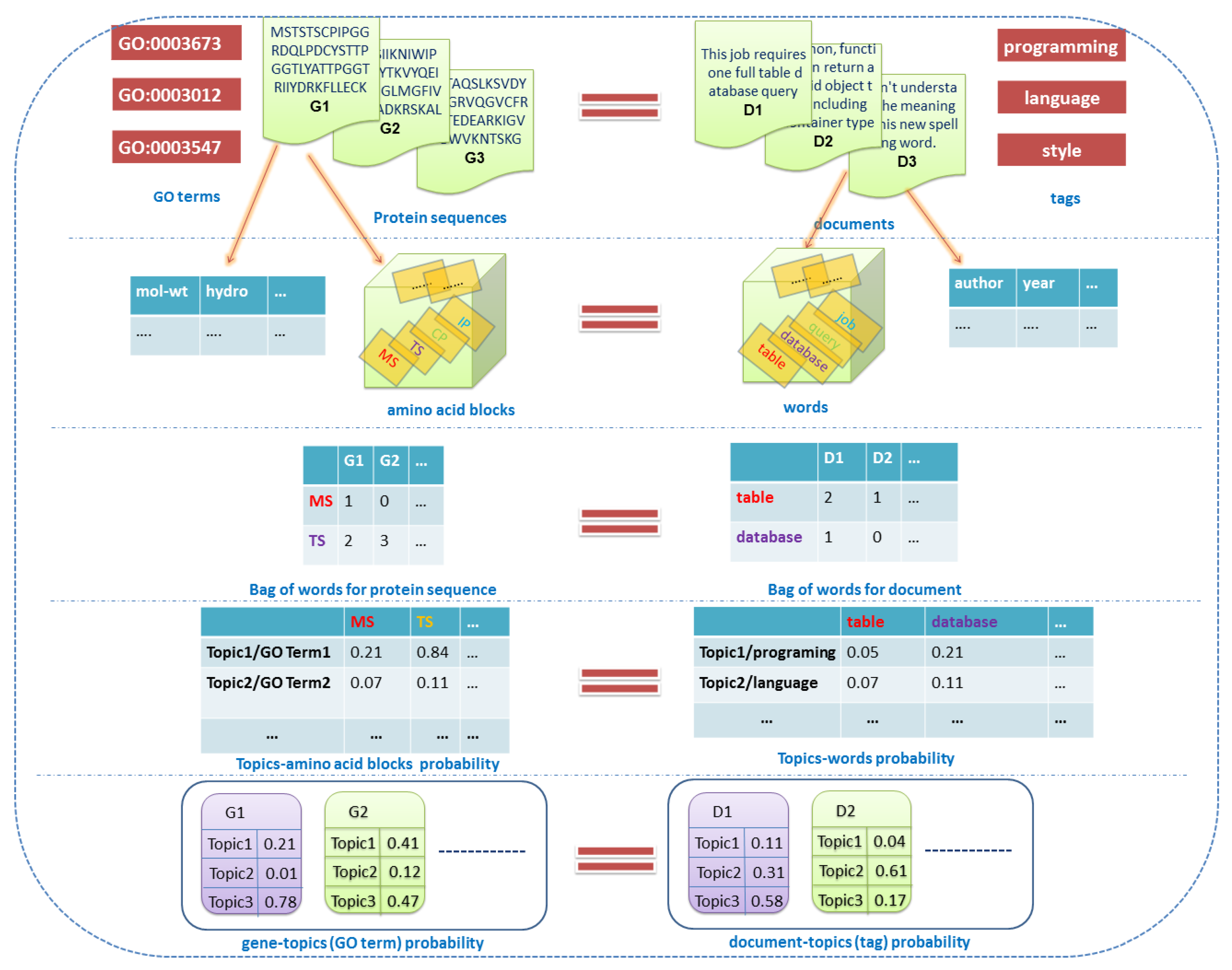
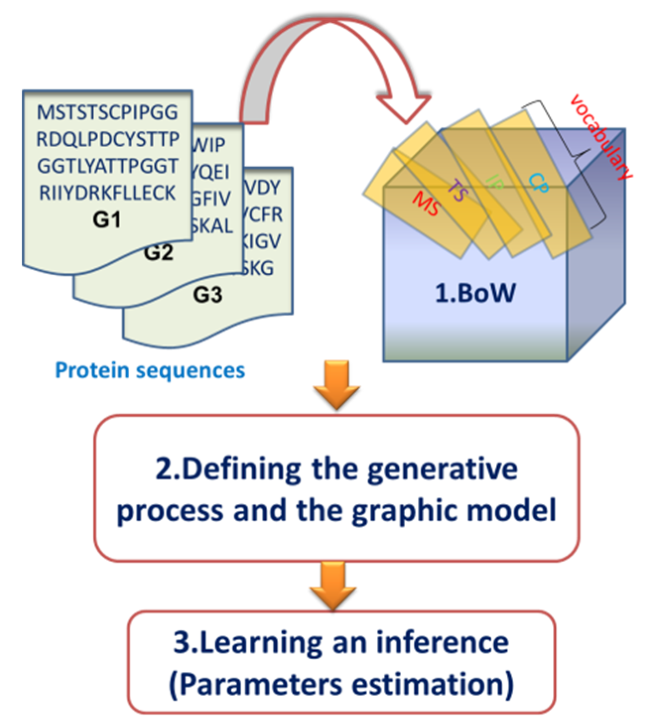
2.2. Overview of the Dirichlet–Multinomial Regression Latent Dirichlet Allocation Topic Modeling Process
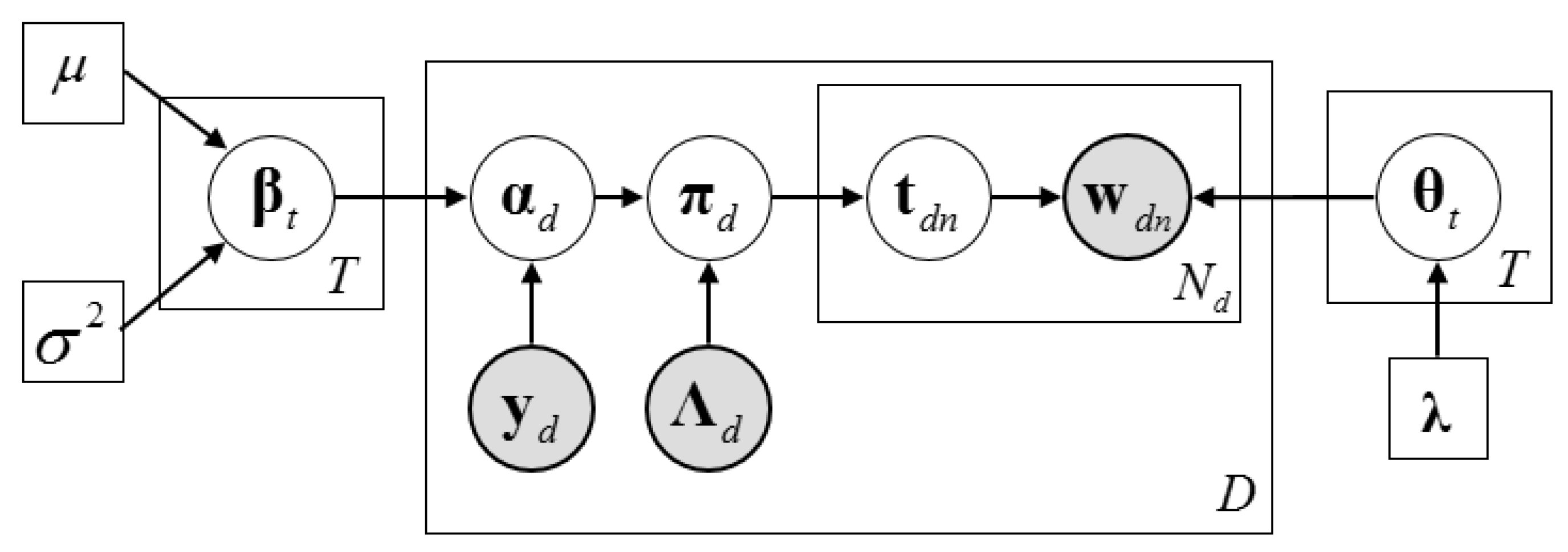
2.3. Description of the Dirichlet–Multinomial Regression Latent Dirichlet Allocation Model
2.4. Inference Algorithm of Dirichlet–Multinomial Regression Latent Dirichlet Allocation
2.4.1. The Collapsed Construction of Dirichlet–Multinomial Regression Latent Dirichlet Allocation
2.4.2. The Optimization of the Feature Parameters of Dirichlet–Multinomial Regression Latent Dirichlet Allocation
2.4.3. The Collapsed Gibbs Sampling Algorithm of the Dirichlet–Multinomial Regression Latent Dirichlet Allocation
2.4.4. The Collapsed Variable Bayesian Inference Algorithm of the Dirichlet–Multinomial Regression Latent Dirichlet Allocation
3. Materials and Results
3.1. Dataset
3.2. Parameter Settings and Evaluation Criterias
3.3. The Impact of Word Length on Model Performance
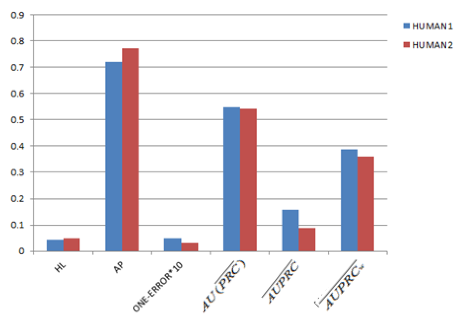
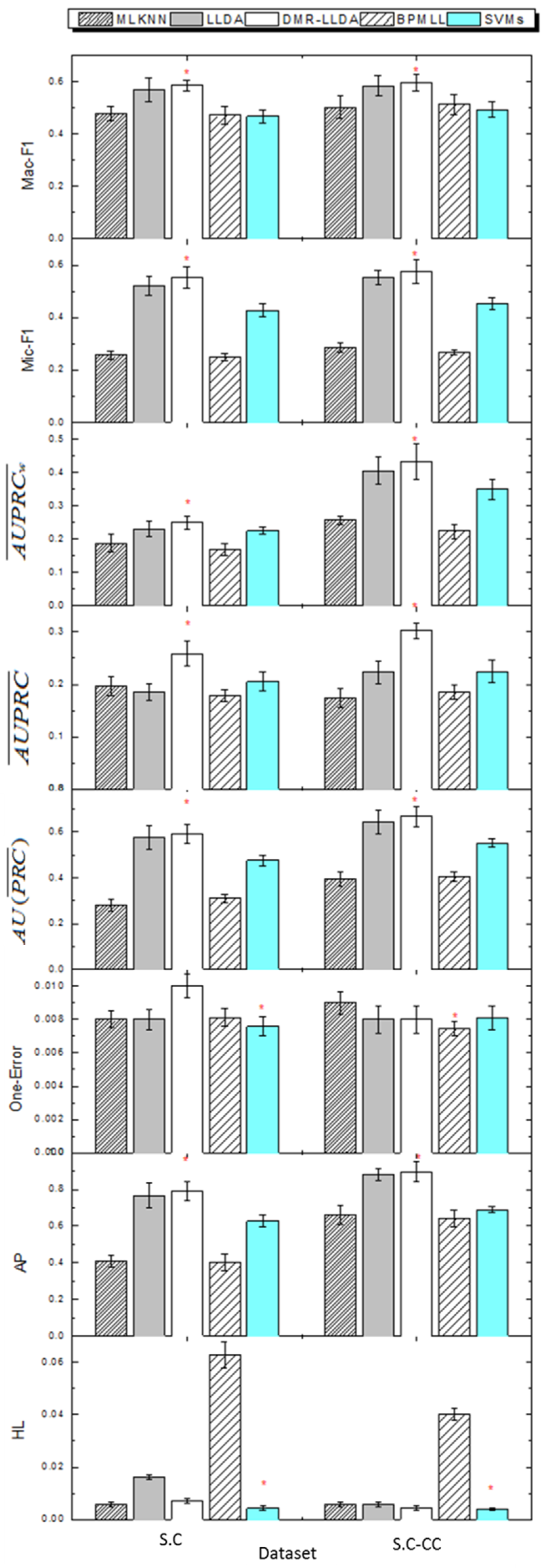
3.4. Gene Function Prediction with Cross Validation
3.5. The Impact on Prior Parameters of Feature Variables
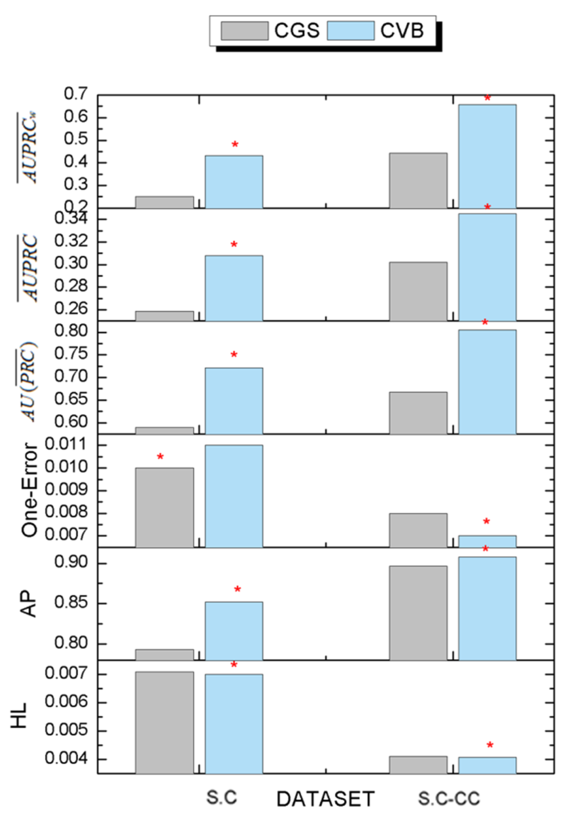
3.6. The Comparison Results of Inference Algorithms
4. Conclusions
Author Contributions
Funding
Acknowledgments
Conflicts of Interest
References
- Pandey, G.; Kumar, V.; Steinbach, M. Computational Approaches for Gene Function Prediction: A Survey; Department of Computer Science and Engineering, University of Minnesota: Minneapolis, MN, USA, 2006. [Google Scholar]
- Altschul, S.F.; Gish, W.; Miller, W.; Myers, E.W.; Lipman, D.J. Basic local alignment search tool. J. Mol. Biol. 1990, 215, 403–410. [Google Scholar] [CrossRef]
- Zacharaki, E.I. Prediction of gene function using a deep convolutional neural network ensemble. PeerJ Comput. Sci. 2017, 3, e124. [Google Scholar] [CrossRef]
- Ofer, D.; Linial, M. ProFET: Feature engineering captures high-level protein functions. Bioinformatics 2015, 31, 3429–3436. [Google Scholar] [CrossRef] [PubMed]
- Yu, G.; Rangwala, H.; Domeniconi, C.; Zhang, G.; Zhang, Z. Predicting gene function using multiple kernels. IEEE/ACM Trans. Comput. Biol. Bioinform. 2015, 12, 219–233. [Google Scholar] [PubMed]
- Cao, R.; Cheng, J. Integrated protein function prediction by mining function associations, sequences, and protein-protein and gene-gene interaction networks. Methods 2016, 93, 84–91. [Google Scholar] [CrossRef] [PubMed]
- Vascon, S.; Frasca, M.; Tripodi, R.; Valentini, G.; Pelillo, M. Protein Function Prediction as a Graph-Transduction Game. Pattern Recogn. Lett. 2018. [Google Scholar] [CrossRef]
- Radivojac, P.; Clark, W.T.; Oron, T.R.; Schnoes, A.M.; Wittkop, T.; Sokolov, A.; Graim, K.; Funk, C.; Verspoor, K.; Ben-Hur, A.; et al. A large-scale evaluation of computational gene function prediction. Nat. Methods 2013, 10, 221–227. [Google Scholar] [CrossRef] [PubMed]
- Shehu, A.; Barbará, D.; Molloy, K. A Survey of Computational Methods for Gene Function Prediction. Big Data Analytics in Genomics; Springer International Publishing: New York, NY, USA, 2016; pp. 225–298. [Google Scholar]
- Lobb, B.; Doxey, A.C. Novel function discovery through sequence and structural data mining. Curr. Opin. Struct. Biol. 2016, 38, 53–61. [Google Scholar] [CrossRef] [PubMed]
- Njah, H.; Jamoussi, S.; Mahdi, W.; Elati, M. A Bayesian approach to construct Context-Specific Gene Ontology: Application to protein function prediction. In Proceedings of the 2016 IEEE Conference on Computational Intelligence in Bioinformatics and Computational Biology (CIBCB), Chiang Mai, Tailand, 5–7 October 2016. [Google Scholar]
- Vens, C.; Struyf, J.; Schietgat, L.; Džeroski, S.; Blockeel, H. Decision trees for hierarchical multi-label classification. Mach. Learn. 2008, 73, 185–214. [Google Scholar] [CrossRef]
- Liu, L.; Tang, L.; He, L.; Yao, S.; Zhou, W. Predicting gene function via multi-label supervised topic model on gene ontology. Biotechnol. Biotechnol. Equip. 2017, 31, 1–9. [Google Scholar] [CrossRef]
- Ramage, D.; Hall, D.; Nallapati, R.; Nallapati, R.; Manning, C. LLDA: A supervised topic model for credit attribution in multi-Lcorpora. In Proceedings of the Conference on Empirical Methods in Natural Language Processing, EMNLP 2009, Singapore, 6–7 August 2009; pp. 248–256. [Google Scholar]
- Mimno, D.; Mccallum, A. Topic Models Conditioned on Arbitrary Features with Dirichlet-Multinomial Regression; University of Massachusetts: Amherst, MA, USA, 2012; pp. 411–418. [Google Scholar]
- La Rosa, M.; Fiannaca, A.; Rizzo, R.; Urso, A. Probabilistic topic modeling for the analysis and classification of genomic sequences. BMC Bioinform. 2015, 16, S2. [Google Scholar] [CrossRef] [PubMed]
- Casella, G.; George, E.I. Explaining the Gibbs Sampler. Am. Stat. 1992, 46, 167–174. [Google Scholar]
- Blei, D.M.; Kucukelbir, A.; Mcauliffe, J.D. Variational Inference: A Review for Statisticians. J. Am. Stat. Assoc. 2018, 112, 859–877. [Google Scholar] [CrossRef]
- Tai, F.; Lin, H.T. Multilabel Classification with Principal Label Space Transformation. Neural Comput. 2012, 24, 2508. [Google Scholar] [CrossRef] [PubMed]
- Sun, Y.; Ye, S.; Sun, Y.; Kameda, T. Improved algorithms for exact and approximate Boolean matrix decomposition. In Proceedings of the IEEE International Conference on Data Science and Advanced Analytics (DSAA), Paris, France, 19–21 October 2015; pp. 1–10. [Google Scholar]
- Yang, Y. Research on Biological Sequence Classification Based on Machine Learning Methods; Shanghai Jiao Tong University: Shanghai, China, 2009. [Google Scholar]
- Minling, Z.; Zhihua, Z. ML-KNN: A lazy learning approach to multi-label learning. Pattern Recogn. 2007, 40, 2038–2048. [Google Scholar]
- Zhang, M.L.; Zhou, Z.H. Multilabel neural networks with applications to functional genomics and text categorization. IEEE Trans. Knowl. Data Eng. 2006, 18, 1338–1351. [Google Scholar] [CrossRef]
- Tsoumakas, G.; Katakis, I.; Vlahavas, I. Mining multi-label data. Data Mining and Knowledge Discovery Handbook; Springer: New York, NY, USA, 2009; pp. 667–685. [Google Scholar]
- Fan, R.E.; Chang, K.W.; Hsieh, C.J.; Wang, X.R.; Lin, C.J. LIBLINEAR: A Library for Large Linear Classification. J. Mach. Learn. Res. 2008, 9, 1871–1874. [Google Scholar]


| CVB algorithm of DMR-LLDA | |
| 1 | Initialize global variational parameters |
| 2 | While the number of iterations or is not converged do |
| 3 | For do |
| 4 | Initialize local variational parameters to constant |
| 5 | Repeat (the local variational inference of gene ) |
| 6 | |
| 7 | Update and by Equations (29)~(30) |
| 8 | |
| 9 | Until is converged: |
| 10 | End For |
| 11 | , , and by Equations (31)~(34) |
| 12 | Update by Equation (21) |
| 13 | End while |
| CVB0 algorithm of DMR-LLDA | |
| 1 | Initialize global variational parameters |
| 2 | While the number of iterations or is not converged do |
| 3 | For do |
| 4 | Initialize local variational parameters to constant |
| 5 | Repeat: (the local variational inference of gene ) |
| 6 | |
| 7 | |
| 8 | |
| 9 | Until is converged: |
| 10 | End For |
| 11 | , |
| 12 | Update by Equation (21) |
| 13 | End while |
| Dataset | ||||
|---|---|---|---|---|
| S.C | 1692 | 400 | 4133 | 1538 |
| S.C-CC | 547 | 319 |
| Feature Name | Notation | Type |
|---|---|---|
| molecular weight | mol_wt | Integer |
| isoelectric point | theo_pI | Real numbers |
| average coefficients of hydrophilic | hydro | Real numbers |
| number of exons | position | Integer |
| adaptability index of codon | Cai | Real numbers |
| number of motifs | motifs | Integer |
| ORF number of chromosomes | chromosome | Integer |
| Dataset | |||
|---|---|---|---|
| Human1 | 4962 | 5297 | 1477 |
| Human2 | 400 |
| The words under topic when mol_wt = 49629.3, theo_pI = 8.96, hydro = 0.1, position = 1, Cai = 0.17, motifs = 2, chromosome = 16 | |
| 1.88 | GM IH LH VH LK IG GC IC AK VM FG AM LW IK VG VW FC IG FH GK |
| 1.32 | LM ST SM LT KM LL IM KL LF SL EM LP DM IT LK EF KT LE SK SP |
| 0.79 | GH VC AC KC GC AL GM LH AH AF AM VW AW GW EC KH TH GF AT GT |
| 0.64 | IL VG GE FM YK QW YM VW GP TL KT LW RP LQ IR FH NW NX FS PM |
| 0.23 | TT SV TV ST SW SQ TQ PT PV IV SP TM CT QT AV TP TC SC VV NV |
| The words under topic when mol_wt = 85873.7, theo_pI = 9.74, hydro=0.664 position = 1, Cai = 0.1, motifs = 2, chromosome = 16 | |
| 4.23 | KR TF KE QS LW EW DM YF QT SM LX SF IN QW LR VL VS QG MC QC |
| 3.77 | LM SM LS RC DW EM LE QT LV EW FM QI RM NE DT IE FT AR QC GP |
| 0.23 | QM KR AP EF LF QR HP EC RE RF DS VE EW KF FE LT TL QV QC AR |
| 0.11 | CF PI ED QY GQ HN RI HD HI SN YQ TQ PW RH YL PQ PN SI QE RS |
| 0.09 | SW VF NW AC DF TW EQ LW EH MC DM AW PS GV VQ AQ ID TG RF VE |
© 2019 by the authors. Licensee MDPI, Basel, Switzerland. This article is an open access article distributed under the terms and conditions of the Creative Commons Attribution (CC BY) license (http://creativecommons.org/licenses/by/4.0/).
Share and Cite
Liu, L.; Tang, L.; Jin, X.; Zhou, W. A Multi-Label Supervised Topic Model Conditioned on Arbitrary Features for Gene Function Prediction. Genes 2019, 10, 57. https://doi.org/10.3390/genes10010057
Liu L, Tang L, Jin X, Zhou W. A Multi-Label Supervised Topic Model Conditioned on Arbitrary Features for Gene Function Prediction. Genes. 2019; 10(1):57. https://doi.org/10.3390/genes10010057
Chicago/Turabian StyleLiu, Lin, Lin Tang, Xin Jin, and Wei Zhou. 2019. "A Multi-Label Supervised Topic Model Conditioned on Arbitrary Features for Gene Function Prediction" Genes 10, no. 1: 57. https://doi.org/10.3390/genes10010057
APA StyleLiu, L., Tang, L., Jin, X., & Zhou, W. (2019). A Multi-Label Supervised Topic Model Conditioned on Arbitrary Features for Gene Function Prediction. Genes, 10(1), 57. https://doi.org/10.3390/genes10010057