
A Meta-Review of Spatial Transcriptomics Analysis Software


Abstract
1. Introduction
2. Tissue Architecture Identification
3. Spatially Variable Gene Discovery
4. Cell–Cell Communication Analysis
5. Deconvolution
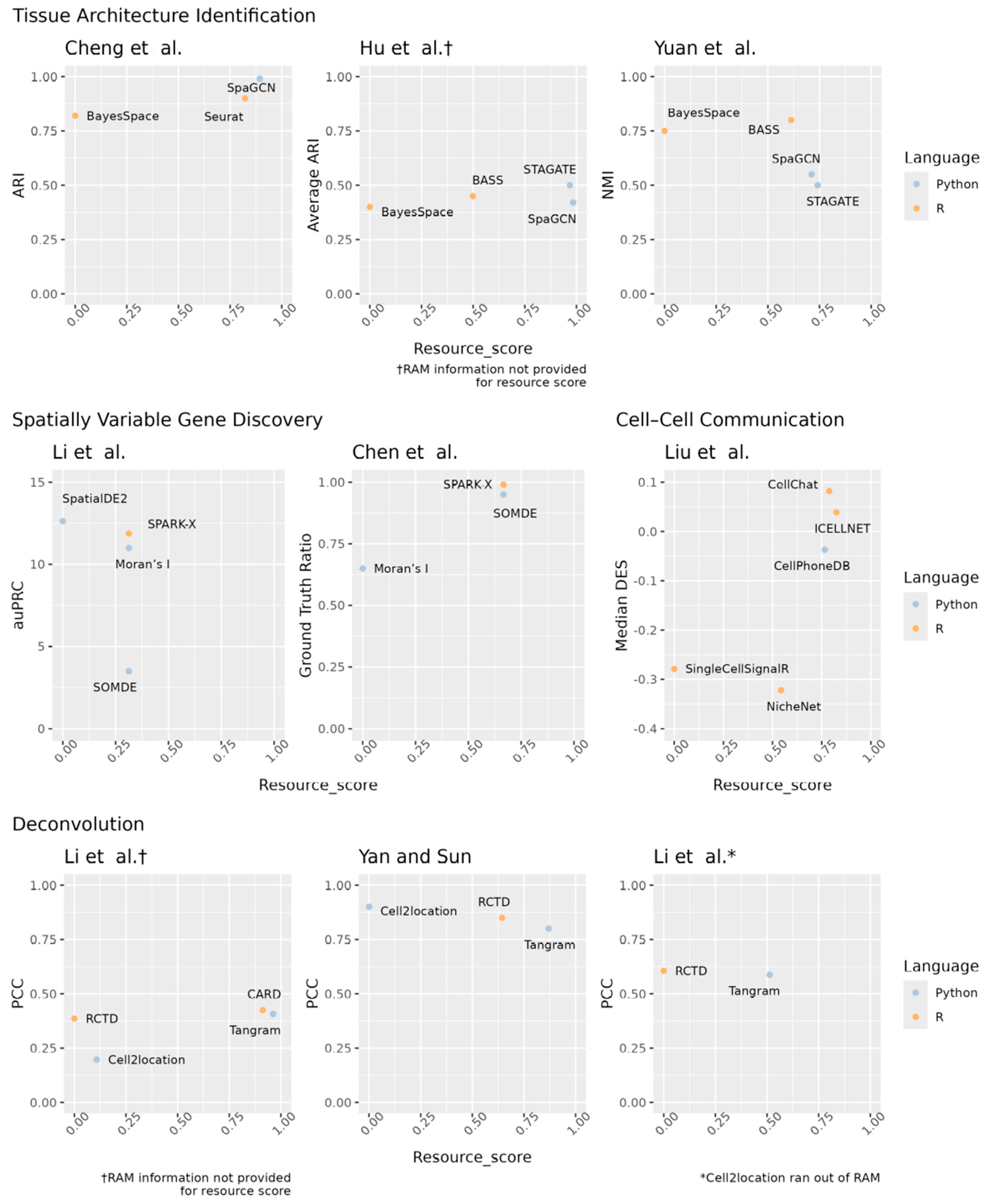
6. Computing Resource Requirements and Accuracy Metrics
7. Conclusions
Author Contributions
Funding
Data Availability Statement
Conflicts of Interest
Abbreviations
| NGS | Next-generation sequencing |
| scRNA-seq | Single-cell RNA-seq |
| ST | Spatial transcriptomics |
| SVG | Spatially variable gene |
| CCC | Cell–cell communication |
| H&E | Hematoxylin and Eosin |
| HVG | Highly variable gene |
| FDR | False discovery rate |
| DES | Distance enrichment score |
References
- Emrich, S.J.; Barbazuk, W.B.; Li, L.; Schnable, P.S. Gene Discovery and Annotation Using LCM-454 Transcriptome Sequencing. Genome Res. 2007, 17, 69–73. [Google Scholar] [CrossRef] [PubMed]
- Wang, Z.; Gerstein, M.; Snyder, M. RNA-Seq: A Revolutionary Tool for Transcriptomics. Nat. Rev. Genet. 2009, 10, 57–63. [Google Scholar] [CrossRef]
- Haque, A.; Engel, J.; Teichmann, S.A.; Lönnberg, T. A Practical Guide to Single-Cell RNA-Sequencing for Biomedical Research and Clinical Applications. Genome Med. 2017, 9, 75. [Google Scholar] [CrossRef] [PubMed]
- Choi, J.R.; Yong, K.W.; Choi, J.Y.; Cowie, A.C. Single-Cell RNA Sequencing and Its Combination with Protein and DNA Analyses. Cells 2020, 9, 1130. [Google Scholar] [CrossRef]
- Williams, C.G.; Lee, H.J.; Asatsuma, T.; Vento-Tormo, R.; Haque, A. An Introduction to Spatial Transcriptomics for Biomedical Research. Genome Med. 2022, 14, 68. [Google Scholar] [CrossRef] [PubMed]
- Rao, A.; Barkley, D.; França, G.S.; Yanai, I. Exploring Tissue Architecture Using Spatial Transcriptomics. Nature 2021, 596, 211–220. [Google Scholar] [CrossRef]
- Liang, G.; Yin, H.; Ding, F. Technical Advances and Applications of Spatial Transcriptomics. GEN Biotechnol. 2023, 2, 384–398. [Google Scholar] [CrossRef]
- Tian, L.; Chen, F.; Macosko, E.Z. The Expanding Vistas of Spatial Transcriptomics. Nat. Biotechnol. 2023, 41, 773–782. [Google Scholar] [CrossRef]
- Hu, Y.; Zhao, Y.; Schunk, C.T.; Ma, Y.; Derr, T.; Zhou, X.M. ADEPT: Autoencoder with differentially expressed genes and imputation for robust spatial transcriptomics clustering. iScience 2023, 26, 106792. [Google Scholar] [CrossRef]
- Singhal, V.; Chou, N.; Lee, J.; Yue, Y.; Liu, J.; Chock, W.K.; Lin, L.; Chang, Y.-C.; Teo, E.M.L.; Aow, J.; et al. BANKSY unifies cell typing and tissue domain segmentation for scalable spatial omics data analysis. Nat. Genet. 2024, 56, 431–441. [Google Scholar] [CrossRef]
- Li, Z.; Zhou, X. BASS: Multi-scale and multi-sample analysis enables accurate cell type clustering and spatial domain detection in spatial transcriptomic studies. Genome Biol. 2022, 23, 168. [Google Scholar] [CrossRef]
- Zhao, E.; Stone, M.R.; Ren, X.; Guenthoer, J.; Smythe, K.S.; Pulliam, T.; Williams, S.R.; Uytingco, C.R.; Taylor, S.E.B.; Nghiem, P.; et al. Spatial Transcriptomics at Subspot Resolution with BayesSpace. Nat. Biotechnol. 2021, 39, 1375–1384. [Google Scholar] [CrossRef]
- Li, J.; Chen, S.; Pan, X.; Yuan, Y.; Shen, H.-B. Cell Clustering for Spatial Transcriptomics Data with Graph Neural Networks. Nat. Comput. Sci. 2022, 2, 399–408. [Google Scholar] [CrossRef] [PubMed]
- Zeng, Y.; Yin, R.; Luo, M.; Chen, J.; Pan, Z.; Lu, Y.; Yu, W.; Yang, Y. Deciphering spatial domains by integrating histopathological image and transcriptomics via contrastive learning. bioRxiv 2022. bioRxiv:2022.09.30.510297. [Google Scholar] [CrossRef]
- Zong, Y.; Yu, T.; Wang, X.; Wang, Y.; Hu, Z.; Li, Y. conST: An interpretable multi-modal contrastive learning framework for spatial transcriptomics. bioRxiv 2022. bioRxiv:2022.01.14.476408. [Google Scholar] [CrossRef]
- Xu, C.; Jin, X.; Wei, S.; Wang, P.; Luo, M.; Xu, Z.; Yang, W.; Cai, Y.; Xiao, L.; Lin, X.; et al. DeepST: Identifying spatial domains in spatial transcriptomics by deep learning. Nucleic Acids Res. 2022, 50, e131. [Google Scholar] [CrossRef]
- Liu, W.; Liao, X.; Yang, Y.; Lin, H.; Yeong, J.; Zhou, X.; Shi, X.; Liu, J. Joint dimension reduction and clustering analysis of single-cell RNA-seq and spatial transcriptomics data. Nucleic Acids Res. 2022, 50, e72. [Google Scholar] [CrossRef] [PubMed]
- Jones, A.; Townes, F.W.; Li, D.; Engelhardt, B.E. Alignment of spatial genomics data using deep Gaussian processes. Nat. Methods 2023, 20, 1379–1387. [Google Scholar] [CrossRef]
- Long, Y.; Ang, K.S.; Li, M.; Chong, K.L.K.; Sethi, R.; Zhong, C.; Xu, H.; Ong, Z.; Sachaphibulkij, K.; Chen, A.; et al. Spatially informed clustering, integration, and deconvolution of spatial transcriptomics with GraphST. Nat. Commun. 2023, 14, 1155. [Google Scholar] [CrossRef]
- Zeira, R.; Land, M.; Strzalkowski, A.; Raphael, B.J. Alignment and integration of spatial transcriptomics data. Nat. Methods 2022, 19, 567–575. [Google Scholar] [CrossRef]
- Liu, X.; Zeira, R.; Raphael, B.J. Partial alignment of multislice spatially resolved transcriptomics data. Genome Res. 2023, 33, 1124–1132. [Google Scholar] [CrossRef] [PubMed]
- Liu, W.; Liao, X.; Luo, Z.; Yang, Y.; Lau, M.C.; Jiao, Y.; Shi, X.; Zhai, W.; Ji, H.; Yeong, J.; et al. Probabilistic embedding, clustering, and alignment for integrating spatial transcriptomics data with PRECAST. Nat. Commun. 2023, 14, 296. [Google Scholar] [CrossRef]
- Xu, H.; Fu, H.; Long, Y.; Ang, K.S.; Sethi, R.; Chong, K.; Li, M.; Uddamvathanak, R.; Lee, H.K.; Ling, J.; et al. Unsupervised spatially embedded deep representation of spatial transcriptomics. Genome Med. 2024, 16, 12. [Google Scholar] [CrossRef] [PubMed]
- Ren, H.; Walker, B.L.; Cang, Z.; Nie, Q. Identifying multicellular spatiotemporal organization of cells with SpaceFlow. Nat. Commun. 2022, 13, 4076. [Google Scholar] [CrossRef] [PubMed]
- Xu, H.; Wang, S.; Fang, M.; Luo, S.; Chen, C.; Wan, S.; Wang, R.; Tang, M.; Xue, T.; Li, B.; et al. SPACEL: Deep learning-based characterization of spatial transcriptome architectures. Nat. Commun. 2023, 14, 7603. [Google Scholar] [CrossRef]
- Shang, L.; Zhou, X. Spatially aware dimension reduction for spatial transcriptomics. Nat. Commun. 2022, 13, 7203. [Google Scholar] [CrossRef] [PubMed]
- Guo, T.; Yuan, Z.; Pan, Y.; Wang, J.; Chen, F.; Zhang, M.Q.; Li, X. SPIRAL: Integrating and aligning spatially resolved transcriptomics data across different experiments, conditions, and technologies. Genome Biol. 2023, 24, 241. [Google Scholar] [CrossRef]
- Dong, K.; Zhang, S. Deciphering Spatial Domains from Spatially Resolved Transcriptomics with an Adaptive Graph Attention Auto-Encoder. Nat. Commun. 2022, 13, 1739. [Google Scholar] [CrossRef]
- Clifton, K.; Anant, M.; Aihara, G.; Atta, L.; Aimiuwu, O.K.; Kebschull, J.M.; Miller, M.I.; Tward, D.; Fan, J. STalign: Alignment of spatial transcriptomics data using diffeomorphic metric mapping. Nat. Commun. 2023, 14, 8123. [Google Scholar] [CrossRef]
- Zhou, X.; Dong, K.; Zhang, S. Integrating spatial transcriptomics data across different conditions, technologies and developmental stages. Nat. Comput. Sci. 2023, 3, 894–906. [Google Scholar] [CrossRef]
- Wolf, F.A.; Angerer, P.; Theis, F.J. SCANPY: Large-scale single-cell gene expression data analysis. Genome Biol. 2018, 19, 15. [Google Scholar] [CrossRef] [PubMed]
- Traag, V.A.; Waltman, L.; Van Eck, N.J. From Louvain to Leiden: Guaranteeing well-connected communities. Sci. Rep. 2019, 9, 5233. [Google Scholar] [CrossRef] [PubMed]
- Cang, Z.; Ning, X.; Nie, A.; Xu, M.; Zhang, J. SCAN-IT: Domain Segmentation of Spatial Transcriptomics images by Graph Neural Network. BMVC 2021, 32, 406. [Google Scholar] [CrossRef]
- Pham, D.; Tan, X.; Balderson, B.; Xu, J.; Grice, L.F.; Yoon, S.; Willis, E.F.; Tran, M.; Lam, P.Y.; Raghubar, A.; et al. Robust mapping of spatiotemporal trajectories and cell–cell interactions in healthy and diseased tissues. Nat. Commun. 2023, 14, 7739. [Google Scholar] [CrossRef]
- Cheng, A.; Hu, G.; Li, W.V. Benchmarking Cell-Type Clustering Methods for Spatially Resolved Transcriptomics Data. Brief. Bioinform. 2022, 24, bbac475. [Google Scholar] [CrossRef] [PubMed]
- Hu, Y.; Xie, M.; Li, Y.; Rao, M.; Shen, W.; Luo, C.; Qin, H.; Baek, J.; Zhou, X.M. Benchmarking Clustering, Alignment, and Integration Methods for Spatial Transcriptomics. Genome Biol. 2024, 25, 212. [Google Scholar] [CrossRef]
- Yuan, Z.; Zhao, F.; Lin, S.; Zhao, Y.; Yao, J.; Cui, Y.; Zhang, X.-Y.; Zhao, Y. Benchmarking Spatial Clustering Methods with Spatially Resolved Transcriptomics Data. Nat. Methods 2024, 21, 712–722. [Google Scholar] [CrossRef]
- Hu, J.; Li, X.; Coleman, K.; Schroeder, A.; Ma, N.; Irwin, D.J.; Lee, E.B.; Shinohara, R.T.; Li, M. SpaGCN: Integrating Gene Expression, Spatial Location and Histology to Identify Spatial Domains and Spatially Variable Genes by Graph Convolutional Network. Nat. Methods 2021, 18, 1342–1351. [Google Scholar] [CrossRef]
- Hao, Y.; Stuart, T.; Kowalski, M.H.; Choudhary, S.; Hoffman, P.; Hartman, A.; Srivastava, A.; Molla, G.; Madad, S.; Fernandez-Granda, C.; et al. Dictionary Learning for Integrative, Multimodal and Scalable Single-Cell Analysis. Nat. Biotechnol. 2024, 42, 293–304. [Google Scholar] [CrossRef]
- Li, Q.; Zhang, M.; Xie, Y.; Xiao, G. Bayesian modeling of spatial molecular profiling data via Gaussian process. Bioinformatics 2021, 37, 4129–4136. [Google Scholar] [CrossRef]
- BinTayyash, N.; Georgaka, S.; John, S.T.; Ahmed, S.; Boukouvalas, A.; Hensman, J.; Rattray, M. Non-parametric modelling of temporal and spatial counts data from RNA-seq experiments. Bioinformatics 2021, 37, 3788–3795. [Google Scholar] [CrossRef] [PubMed]
- Svensson, V.; Teichmann, S.A.; Stegle, O. SpatialDE: Identification of Spatially Variable Genes. Nat. Methods 2018, 15, 343–346. [Google Scholar] [CrossRef] [PubMed]
- Dries, R.; Zhu, Q.; Dong, R.; Eng, C.-H.L.; Li, H.; Liu, K.; Fu, Y.; Zhao, T.; Sarkar, A.; Bao, F.; et al. Giotto: A toolbox for integrative analysis and visualization of spatial expression data. Genome Biol. 2021, 22, 78. [Google Scholar] [CrossRef]
- Miller, B.F.; Bambah-Mukku, D.; Dulac, C.; Zhuang, X.; Fan, J. Characterizing spatial gene expression heterogeneity in spatially resolved single-cell transcriptomic data with nonuniform cellular densities. Genome Res. 2021, 31, 1843–1855. [Google Scholar] [CrossRef]
- Hao, Y.; Hao, S.; Andersen-Nissen, E.; Mauck, W.M.; Zheng, S.; Butler, A.; Lee, M.J.; Wilk, A.J.; Darby, C.; Zager, M.; et al. Integrated analysis of multimodal single-cell data. Cell 2021, 184, 3573–3587.e29. [Google Scholar] [CrossRef] [PubMed]
- Weber, L.M.; Saha, A.; Datta, A.; Hansen, K.D.; Hicks, S.C. nnSVG for the scalable identification of spatially variable genes using nearest-neighbor Gaussian processes. Nat. Commun. 2023, 14, 4059. [Google Scholar] [CrossRef]
- Hao, M.; Hua, K.; Zhang, X. SOMDE: A Scalable Method for Identifying Spatially Variable Genes with Self-Organizing Map. Bioinformatics 2021, 37, 4392–4398. [Google Scholar] [CrossRef]
- Zhu, J.; Sun, S.; Zhou, X. SPARK-X: Non-Parametric Modeling Enables Scalable and Robust Detection of Spatial Expression Patterns for Large Spatial Transcriptomic Studies. Genome Biol. 2021, 22, 184. [Google Scholar] [CrossRef]
- Li, Z.; Patel, Z.M.; Song, D.; Yan, G.; Li, J.J.; Pinello, L. Benchmarking Computational Methods to Identify Spatially Variable Genes and Peaks. bioRxiv 2023. bioRxiv:2023.12.02.569717. [Google Scholar] [CrossRef]
- Chen, C.; Kim, H.J.; Yang, P. Evaluating Spatially Variable Gene Detection Methods for Spatial Transcriptomics Data. Genome Biol. 2024, 25, 18. [Google Scholar] [CrossRef]
- MORAN, P.A.P. Notes on Continuous Stochastic Phenomena. Biometrika 1950, 37, 17–23. [Google Scholar] [CrossRef]
- Zhou, X.; Franklin, R.A.; Adler, M.; Jacox, J.B.; Bailis, W.; Shyer, J.A.; Flavell, R.A.; Mayo, A.; Alon, U.; Medzhitov, R. Circuit Design Features of a Stable Two-Cell System. Cell 2018, 172, 744–757.e17. [Google Scholar] [CrossRef] [PubMed]
- Hu, M.; Polyak, K. Microenvironmental Regulation of Cancer Development. Curr. Opin. Genet. Dev. 2008, 18, 27–34. [Google Scholar] [CrossRef] [PubMed]
- Shao, X.; Lu, X.; Liao, J.; Chen, H.; Fan, X. New Avenues for Systematically Inferring Cell-Cell Communication: Through Single-Cell Transcriptomics Data. Protein Cell 2020, 11, 866–880. [Google Scholar] [CrossRef] [PubMed]
- Armingol, E.; Officer, A.; Harismendy, O.; Lewis, N.E. Deciphering Cell–Cell Interactions and Communication from Gene Expression. Nat. Rev. Genet. 2021, 22, 71–88. [Google Scholar] [CrossRef]
- Ma, F.; Zhang, S.; Song, L.; Wang, B.; Wei, L.; Zhang, F. Applications and Analytical Tools of Cell Communication Based on Ligand-Receptor Interactions at Single Cell Level. Cell Biosci. 2021, 11, 121. [Google Scholar] [CrossRef]
- Sekar, R.B.; Periasamy, A. Fluorescence Resonance Energy Transfer (FRET) Microscopy Imaging of Live Cell Protein Localizations. J. Cell Biol. 2003, 160, 629–633. [Google Scholar] [CrossRef]
- Jackman, J.A.; Cho, N.-J. Supported Lipid Bilayer Formation: Beyond Vesicle Fusion. Langmuir 2020, 36, 1387–1400. [Google Scholar] [CrossRef]
- Liu, Z.; Sun, D.; Wang, C. Evaluation of Cell-Cell Interaction Methods by Integrating Single-Cell RNA Sequencing Data with Spatial Information. Genome Biol. 2022, 23, 218. [Google Scholar] [CrossRef]
- Jin, S.; Plikus, M.V.; Nie, Q. CellChat for Systematic Analysis of Cell–Cell Communication from Single-Cell Transcriptomics. Nat. Protoc. 2025, 20, 180–219. [Google Scholar] [CrossRef]
- Noël, F.; Massenet-Regad, L.; Carmi-Levy, I.; Cappuccio, A.; Grandclaudon, M.; Trichot, C.; Kieffer, Y.; Mechta-Grigoriou, F.; Soumelis, V. Dissection of Intercellular Communication Using the Transcriptome-Based Framework ICELLNET. Nat. Commun. 2021, 12, 1089. [Google Scholar] [CrossRef] [PubMed]
- Efremova, M.; Vento-Tormo, M.; Teichmann, S.A.; Vento-Tormo, R. CellPhoneDB: Inferring Cell–Cell Communication from Combined Expression of Multi-Subunit Ligand–Receptor Complexes. Nat. Protoc. 2020, 15, 1484–1506. [Google Scholar] [CrossRef]
- Cabello-Aguilar, S.; Alame, M.; Kon-Sun-Tack, F.; Fau, C.; Lacroix, M.; Colinge, J. SingleCellSignalR: Inference of Intercellular Networks from Single-Cell Transcriptomics. Nucleic Acids Res. 2020, 48, e55. [Google Scholar] [CrossRef]
- Browaeys, R.; Saelens, W.; Saeys, Y. NicheNet: Modeling Intercellular Communication by Linking Ligands to Target Genes. Nat. Methods 2020, 17, 159–162. [Google Scholar] [CrossRef]
- Hou, R.; Denisenko, E.; Ong, H.T.; Ramilowski, J.A.; Forrest, A.R.R. Predicting cell-to-cell communication networks using NATMI. Nat. Commun. 2020, 11, 5011. [Google Scholar] [CrossRef]
- Song, Q.; Su, J. DSTG: Deconvoluting spatial transcriptomics data through graph-based artificial intelligence. Brief. Bioinform. 2020, 22, bbaa414. [Google Scholar] [CrossRef] [PubMed]
- Rodriques, S.G.; Stickels, R.R.; Goeva, A.; Martin, C.A.; Murray, E.; Vanderburg, C.R.; Welch, J.; Chen, L.M.; Chen, F.; Macosko, E.Z. Slide-seq: A scalable technology for measuring genome-wide expression at high spatial resolution. Science 2019, 363, 1463–1467. [Google Scholar] [CrossRef] [PubMed]
- Li, H.; Li, H.; Zhou, J.; Gao, X. SD2: Spatially resolved transcriptomics deconvolution through integration of dropout and spatial information. Bioinformatics 2022, 38, 4878–4884. [Google Scholar] [CrossRef]
- Cang, Z.; Nie, Q. Inferring spatial and signaling relationships between cells from single cell transcriptomic data. Nat. Commun. 2020, 11, 2084. [Google Scholar] [CrossRef]
- Danaher, P.; Kim, Y.; Nelson, B.; Griswold, M.; Yang, Z.; Piazza, E.; Beechem, J.M. Advances in mixed cell deconvolution enable quantification of cell types in spatial transcriptomic data. Nat. Commun. 2022, 13, 385. [Google Scholar] [CrossRef]
- Dong, R.; Yuan, G.-C. SpatialDWLS: Accurate deconvolution of spatial transcriptomic data. Genome Biol. 2021, 22, 145. [Google Scholar] [CrossRef] [PubMed]
- Chidester, B.; Zhou, T.; Alam, S.; Ma, J. SpiceMix enables integrative single-cell spatial modeling of cell identity. Nat. Genet. 2023, 55, 78–88. [Google Scholar] [CrossRef] [PubMed]
- Sun, D.; Liu, Z.; Li, T.; Wu, Q.; Wang, C. STRIDE: Accurately decomposing and integrating spatial transcriptomics using single-cell RNA sequencing. Nucleic Acids Res. 2022, 50, e42. [Google Scholar] [CrossRef]
- Kleshchevnikov, V.; Shmatko, A.; Dann, E.; Aivazidis, A.; King, H.W.; Li, T.; Elmentaite, R.; Lomakin, A.; Kedlian, V.; Gayoso, A.; et al. Cell2location Maps Fine-Grained Cell Types in Spatial Transcriptomics. Nat. Biotechnol. 2022, 40, 661–671. [Google Scholar] [CrossRef]
- Lopez, R.; Li, B.; Keren-Shaul, H.; Boyeau, P.; Kedmi, M.; Pilzer, D.; Jelinski, A.; David, E.; Wagner, A.; Addad, Y.; et al. Multi-resolution deconvolution of spatial transcriptomics data reveals continuous patterns of inflammation. bioRxiv 2021. bioRxiv:2021.05.10.443517. [Google Scholar] [CrossRef]
- Moncada, R.; Barkley, D.; Wagner, F.; Chiodin, M.; Devlin, J.C.; Baron, M.; Hajdu, C.H.; Simeone, D.M.; Yanai, I. Integrating microarray-based spatial transcriptomics and single-cell RNA-seq reveals tissue architecture in pancreatic ductal adenocarcinomas. Nat. Biotechnol. 2020, 38, 333–342. [Google Scholar] [CrossRef] [PubMed]
- Cable, D.M.; Murray, E.; Zou, L.S.; Goeva, A.; Macosko, E.Z.; Chen, F.; Irizarry, R.A. Robust Decomposition of Cell Type Mixtures in Spatial Transcriptomics. Nat. Biotechnol. 2022, 40, 517–526. [Google Scholar] [CrossRef]
- Miller, B.F.; Huang, F.; Atta, L.; Sahoo, A.; Fan, J. Reference-free cell type deconvolution of multi-cellular pixel-resolution spatially resolved transcriptomics data. Nat. Commun. 2022, 13, 2339. [Google Scholar] [CrossRef]
- Andersson, A.; Bergenstråhle, J.; Asp, M.; Bergenstråhle, L.; Jurek, A.; Navarro, J.F.; Lundeberg, J. Single-cell and spatial transcriptomics enables probabilistic inference of cell type topography. Commun. Biol. 2020, 3, 565. [Google Scholar] [CrossRef]
- Elosua-Bayes, M.; Nieto, P.; Mereu, E.; Gut, I.; Heyn, H. SPOTlight: Seeded NMF regression to deconvolute spatial transcriptomics spots with single-cell transcriptomes. Nucleic Acids Res. 2021, 49, e50. [Google Scholar] [CrossRef]
- Biancalani, T.; Scalia, G.; Buffoni, L.; Avasthi, R.; Lu, Z.; Sanger, A.; Tokcan, N.; Vanderburg, C.R.; Segerstolpe, Å.; Zhang, M.; et al. Deep Learning and Alignment of Spatially Resolved Single-Cell Transcriptomes with Tangram. Nat. Methods 2021, 18, 1352–1362. [Google Scholar] [CrossRef] [PubMed]
- Lopez, R.; Nazaret, A.; Langevin, M.; Samaran, J.; Regier, J.; Jordan, M.I.; Yosef, N. A joint model of unpaired data from scRNA-seq and spatial transcriptomics for imputing missing gene expression measurements. arXiv 2019, arXiv:1905.02269. [Google Scholar] [CrossRef]
- Welch, J.D.; Kozareva, V.; Ferreira, A.; Vanderburg, C.; Martin, C.; Macosko, E.Z. Single-Cell multi-omic integration compares and contrasts features of brain cell identity. Cell 2019, 177, 1873–1887.e17. [Google Scholar] [CrossRef]
- Nitzan, M.; Karaiskos, N.; Friedman, N.; Rajewsky, N. Gene expression cartography. Nature 2019, 576, 132–137. [Google Scholar] [CrossRef] [PubMed]
- Shengquan, C.; Boheng, Z.; Xiaoyang, C.; Xuegong, Z.; Rui, J. stPlus: A reference-based method for the accurate enhancement of spatial transcriptomics. Bioinformatics 2021, 37 (Suppl. 1), i299–i307. [Google Scholar] [CrossRef]
- Li, H.; Zhou, J.; Li, Z.; Chen, S.; Liao, X.; Zhang, B.; Zhang, R.; Wang, Y.; Sun, S.; Gao, X. A Comprehensive Benchmarking with Practical Guidelines for Cellular Deconvolution of Spatial Transcriptomics. Nat. Commun. 2023, 14, 1548. [Google Scholar] [CrossRef]
- Yan, L.; Sun, X. Benchmarking and Integration of Methods for Deconvoluting Spatial Transcriptomic Data. Bioinformatics 2022, 39, btac805. [Google Scholar] [CrossRef]
- Li, B.; Zhang, W.; Guo, C.; Xu, H.; Li, L.; Fang, M.; Hu, Y.; Zhang, X.; Yao, X.; Tang, M.; et al. Benchmarking Spatial and Single-Cell Transcriptomics Integration Methods for Transcript Distribution Prediction and Cell Type Deconvolution. Nat. Methods 2022, 19, 662–670. [Google Scholar] [CrossRef]
- Tu, J.-J.; Li, H.-S.; Yan, H.; Zhang, X.-F. EnDecon: Cell Type Deconvolution of Spatially Resolved Transcriptomics Data via Ensemble Learning. Bioinformatics. 2023, 39, btac825. [Google Scholar] [CrossRef]
- Aquila. Cheunglab.org. 2024. Available online: https://aquila.cheunglab.org/ (accessed on 11 May 2025).
- Xu, Z.; Wang, W.; Yang, T.; Li, L.; Ma, X.; Chen, J.; Wang, J.; Huang, Y.; Gould, J.; Lu, H.; et al. STOmicsDB: A comprehensive database for spatial transcriptomics data sharing, analysis and visualization. Nucleic Acids Res. 2024, 5, D1053–D1061. [Google Scholar] [CrossRef]
- STOmicsDB: Spatial TranscriptOmics DataBase. 2024. Available online: https://db.cngb.org/stomics/ (accessed on 11 May 2025).
- SOAR: Spatial TranscriptOmics Analysis Resource. Northwestern.edu. 2018. Available online: https://soar.fsm.northwestern.edu/ (accessed on 11 May 2025).


| Author | Software | Accuracy Metric | Dataset | Technology | Computer Environment | |
|---|---|---|---|---|---|---|
| Cheng et al. | BayesSpace (v1.00) DR.SC (v2.9) Giotto-H (v1.0.3) Giotto-HM (v1.0.3) Giotto-KM (v1.0.3) Giotto-LD (v1.0.3) Seurat-LV (v4.0.5) Seurat-LVM V (v4.0.5) | Seurat-SLM V (v4.0.5) SpaCell (v1.0.1) SpaCell-G (v1.0.1) SpaCell-I (v1.0.1) SpaGCN (v1.2.0) SpaGCN+ (v1.2.0) StLearn (v0.3.2) | ARI with annotated datasets as ground truth. Also mean and AD of ARI across replicates. | Mouse olfactory bulb | Spatial Transcriptomics | Information not provided |
| Mouse kidney coronal | 10x Genomics Visium V1 | |||||
| Mouse brain sagittal | 10x Genomics Visium V1 | |||||
| Mouse hypothalamic preoptic | MERFISH | |||||
| Mouse somatosensory cortex | osmFISH | |||||
| Mouse olfactory bulb | Stereo-seq | |||||
| Mouse brain cerebellum | Slide-seq | |||||
| Hu et al. | ADEPT [9] BANKSY [10] BASS [11] BayesSpace [12] CCST [13] ConGI [14] conST [15] DeepST [16] DR.SC [17] GPSA [18] GraphST [19] | PASTE [20] PASTE2 [21] PRECAST [22] SEDR [23] SpaceFlow [24] SPACEL [25] SpaGCN [4] SpatialPCA [26] SPIRAL [27] STAGATE [28] STalign [29] STAligner [30] | ARI, NMI, AMI, and HOM, with annotated and simulated datasets as ground truth. | DLPFC | 10x Genomics Visium V1 | Intel Xeon W-2195 CPU 2.3 GHz 36 CPU cores 256 GB DDR4 RAM Four Quadro RTX A6000 GPUs 48 GB RAM 4608 CUDA cores |
| HBCA1 | 10x Genomics Visium V1 | |||||
| MB2SA | 10x Genomics Visium V1 | |||||
| HER2BT | Spatial Transcriptomics | |||||
| MHPC | Slide-seq V2 | |||||
| Embryo | Stereo-seq | |||||
| MVC | STARmap | |||||
| MPFC | STARmap | |||||
| Yuan et al. | BASS [11] BayesSpace [12] CCST [13] conST [15] GraphST [19] Leiden [31,32] | Louvain [31] SCAN-IT [33] SEDR [23] SpaceFlow [24] SpaGCN [4] STAGATE [28] StLearn [34] | NMI against annotated datasets for ground truth. | DLPFC | 10x Visium | Intel Xeon E5-2683v3 2.00 GHz 14 cores 128 GB RAM NVIDIA TITAN Xp GPU 12 GB RAM |
| Mouse embryo | Stereo-seq | |||||
| Mouse primary cortex | Barista-seq | |||||
| Mouse hypothalamic preoptic | MERFISH | |||||
| Mouse somatosensory cortex | osmFISH | |||||
| Mouse medial prefrontal cortex | STARmap | |||||
| Mouse visual cortex | STARmap* | |||||
| Mouse somatosensory cortex with downsampling or noise addition | Simulated_1 | |||||
| Simulated_2 | ||||||
| Simulated_3 | ||||||
| Simulated_4 | ||||||
| Author | Software | Accuracy Metric | Dataset | Production Method/Technology | Computer Environment | |
|---|---|---|---|---|---|---|
| Li et al. | BOOST-GP [40] GPcounts [41] Moran’s I (Squidpy v1.2.3) nnSVG (v1.2.0) scGCO (v1.1.0) Sepal (Squidpy v1.2.3) SOMDE (v0.1.7) | SpaGCN (v1.2.5) SpaGFT (v0.1.1.4) Spanve {v0.1.0) SPARK (v1.1.1) SPARK-X (v1.1.1) SpatialDE (v1.1.3) SpatialDE2 [42] | Area under the precision–recall curve for calls against simulated data ground truth. | Simulated SVGs | Produced with normal and Gaussian distributions | AMD EPYC 7H12 CPU 64 cores 1 TB RAM A100 GPU 40 GB RAM |
| Simulated non-SVGs | Identity matrix | |||||
| Breast tumor with annotation | GP mixture model, log fold change | |||||
| DLPFC | Manual annotation | |||||
| Chen et al. | Giotto k-means [43] Giotto rank [43] MERINGUE [44] Moran’s I [45] nnSVG [46] SOMDE [47] SPARK-X [48] SpatialDE [42] | Spearman’s correlation between SVG lists returned by software. | Mouse embryo E12 | DbiT-seq, D1 | Standard virtual machine 16 OCPUs 256 GB RAM | |
| Mouse embryo E11 | DbiT-seq, D2 | |||||
| Human osteosarcoma | MERFISH | |||||
| Mouse brain cortex | seqFISH+ | |||||
| Mouse cerebellum | Slide-seqV1 | |||||
| Human kidney cortex | Slide-seqV2 | |||||
| Mouse hippocampus | Slide-seqV2 | |||||
| Mouse brain cortex | SM_Omics, D1 | |||||
| Mouse brain cortex | SM_Omics, D2 | |||||
| Human squamous carcinoma | ST | |||||
| Mouse hippocampus | ST | |||||
| Mouse primary motor cortex | Visium | |||||
| Mouse kidney sham | Visium, D1 | |||||
| Mouse kidney ischemia | Visium, D2 | |||||
| Zebrafish melanoma | Visium | |||||
| Mouse kidney sepsis | Visium | |||||
| Mouse prefrontal cortex | Visium | |||||
| Mouse lymph node | Visium, D1 | |||||
| Mouse MCA205 tumor | Visium, D2 | |||||
| Human prostate | Visium | |||||
| Human breast cancer | Visium, D1 | |||||
| Human breast cancer | Visium, D2 | |||||
| Author | Software | Accuracy Metric | Dataset | Production Method/Technology | Computer Environment |
|---|---|---|---|---|---|
| Liu et al. | CellCall (v.0.0.0.9000) CellChat (v1.0.0) CellPhoneDB (v2) CellPhoneDB (v3) Connectome (v1.0.1) CytoTalk (v4.0.11) Domino (v0.1.1) Giotto (v1.0.4) ICELLNET (v0.99.3) iTALK (v0.1.0) NATMI [65] NicheNet (v1.0.0) scMLnet (v0.1.0) SingleCellSignalR (v1.4.0) stLearn (v0.4.7) | Distance enrichment score (DES): A calculation to quantify the consistency between the expected and observed distance of ligand–receptor pairs. | Human pancreatic ductal adenocarcinoma | ST | AMD EPYC 7552 48 cores 566 GB RAM |
| Human squamous cell carcinoma | Visium V1 | ||||
| Mouse cortex | Visium | ||||
| Human heart | Visium | ||||
| Human intestine | Visium |
| Author | Software | Accuracy Metric | Dataset | Production Method/Technology | Computer Environment |
|---|---|---|---|---|---|
| Li et al. | Berglund E et al. (v0.2.0) CARD (v1.0.0) Cell2location (v0.1) DestVI (s cvi-tools 0.16.0) DSTG [66] NMFReg [67] NovoSpaRc (v0.4.4) RCTD (spacexr 2.0.0) SD2 [68] SpaOTsc [69] SpatialDecon [70] SpatialDWLS [71] Stdeconvolve (v1.0.0) stereoscope (v.03) SpiceMix [72] SPOTlight (v0.99.0) STRIDE [73] Tangram (v1.0.3) | JSD score, RMSE, and PCC against annotated ground truth. | Mouse brain medial pre-optic area | MERFISH | Intel Xeon E5-2680 v3 2.50 GHz 24 cores 528 GB RAM Two Nvidia Quadro M6000 GPUs 24 GB |
| Mouse cortex | seqFISH+ | ||||
| PDAC | ST | ||||
| Mouse brain | Visium | ||||
| Mouse hippocampus | Slide-seqV2 | ||||
| Olfactory bulb | Stereo-seq | ||||
| Zebrafish embryo | Stereo-seq | ||||
| Yan and Sun | Cell2location [74] DestVI [75] DSTG [66] Giotto/Hypergeometric [43] Giotto/PAGEGiotto/rank [43] MIA [76] RCTD [77] Seurat [39] SpatialDecon [70] SpatialDWLS [71] Stdeconvolve [78] stereoscope [79] SPOTlight [80] STRIDE [73] Tangram [81] | RMSE, PCC, and JSD with synthetic datasets as ground truth. | Mouse embryo | Sci-Space | 2.7 GHz 112 cores |
| Li et al. | Cell2location [74] DestVI [75] DSTG [66] gimVI [82] LIGER [83] NovoSpaRc [84] RCTD [77] Seurat [39] SPaOTsc [69] SpatialDWLS [71] stereoscope [79] SPOTlight [80] StPlus [85] STRIDE [73] Tangram [81] | Pearson correlation coefficient between expression vector in ground truth dataset and expression vector in the result predicted by each integration method. | Mouse primary visual cortex (VISp) | BARISTAseq | CPU 2.2 GHz 144 CPU cores NVIDIA Tesla K80 GPU 12 GB RAM |
| Mouse primary visual cortex (VISp) | ExSeq | ||||
| Drosophila embryo | FISH | ||||
| Mouse olfactory bulb | HDST | ||||
| Human MTG | ISS | ||||
| Mouse primary visual cortex (VISp) | ISS | ||||
| Human osteosarcoma | MERFISH | ||||
| Mouse hypothalamic preoptic region | MERFISH | ||||
| Mouse primary motor cortex | MERFISH | ||||
| Mouse primary visual cortex (VISp) | MERFISH | ||||
| Mouse somatosensory cortex | osmFISH | ||||
| Mouse liver | Seq-scope | ||||
| Mouse embryonic | seqFISH | ||||
| Mouse gastrulation | seqFISH | ||||
| Mouse hippocampus | seqFISH | ||||
| Mouse cortex | seqFISH+ | ||||
| Mouse olfactory bulb | seqFISH+ | ||||
| Mouse primary motor cortex | Slide-seq | ||||
| Mouse cerebellum | Slide-seqV2 | ||||
| Mouse hippocampus | Slide-seqV2 | ||||
| Human squamous carcinoma | ST | ||||
| Mouse hippocampus | ST | ||||
| Mouse prefrontal cortex | STARmap | ||||
| Mouse visual cortex | STARmap | ||||
| Human prostate | Visium | ||||
| Mouse brain | Visium | ||||
| Mouse breast cancer | Visium | ||||
| Mouse embryo | Visium | ||||
| Mouse hindlimb muscle | Visium | ||||
| Mouse hippocampus | Visium | ||||
| Mouse kidney | Visium | ||||
| Mouse lymph node | Visium | ||||
| Mouse MCA205 tumor | Visium | ||||
| Mouse prefrontal cortex | Visium | ||||
| Mouse primary motor cortex | Visium | ||||
| Zebrafish melanoma | Visium |
| Tissue Architecture Identification | ||||||
|---|---|---|---|---|---|---|
| Cheng et al. | ||||||
| Software | Dataset | Computer Environment | Time (Min) | RAM (GB) | ARI | |
| BayesSpace (v1.00) | R | Visium with 2696–3353 cells and 31,053 genes | Information not provided | 31.623 | 5.495 | 0.820 |
| SpaGCN (v1.2.0) | Python | <1 | 1.000 | 0.990 | ||
| Seurat (v4.0.5) | R | <1 | 1.778 | 0.900 | ||
| Hu et al. | ||||||
| Software | Dataset | Computer Environment | Time (Min) | RAM (GB) | Average ARI | |
| BASS [11] | R | Visium DLFPC, HBCA1, and MB25A datasets | Intel Xeon W-2195 CPU 2.3 GHz 36 CPU cores 256 GB DDR4 RAM Four Quadro RTX A6000 GPUs 48 GB RAM 4608 CUDA cores | 316.228 | Data not provided | 0.450 |
| BayesSpace [12] | R | 630.957 | Data not provided | 0.400 | ||
| SpaGCN [4] | Python | 10.000 | Ran out of RAM | 0.420 | ||
| STAGATE [28] | Python | 19.953 | Data not provided | 0.500 | ||
| Yuan et al. | ||||||
| Software | Dataset | Computer Environment | Time (Min) | RAM (GB) | NMI | |
| BASS [11] | R | Visium DLFPC | Intel Xeon E5-2683v3 2.00 GHz 14 cores 128 GB RAM NVIDIA TITAN Xp GPU 12 GB RAM | 20.000 | 2.5 | 0.800 |
| BayesSpace [12] | R | 41.667 | 8.5 | 0.750 | ||
| SpaGCN [4] | Python | 16.667 | 1.5 | 0.550 | ||
| STAGATE [28] | Python | 16.667 | <1 | 0.500 | ||
| Spatially Variable Gene Discovery | ||||||
| Li et al. | ||||||
| Software | Dataset | Computer Environment | Time (Min) | RAM (GB) | auPRC | |
| SpatialDE2 [42] | Python | Simulated 100 genes and 40,000 spots | AMD EPYC 7H12 CPU 64 cores 1 TB RAM A100 GPU 40 GB RAM | 45 | 16 | 12.625 |
| SPARK-X (v1.1.1) | R | 45 | 6 | 11.875 | ||
| SOMDE (v0.1.7) | Python | 45 | 6 | 3.500 | ||
| Moran’s I (Squidpy v1.2.3) | Python | 45 | 6 | 11.000 | ||
| Chen et al. | ||||||
| Software | Dataset | Computer Environment | Time (Min) | RAM (GB) | Ratio Returned List to Ground Truth List SVGs | |
| SPARK-X [48] | R | Combination of Visium datasets with ~12,000 genes and ~200 spots | Standard virtual machine 16 OCPUs 256 GB RAM | 10 | <1 | 0.990 |
| SOMDE [47] | Python | 10 | <1 | 0.950 | ||
| Moran’s I [45] | Python | 30 | 3 | 0.650 | ||
| Cell–Cell Communication Analysis | ||||||
| Liu et al. | ||||||
| Software | Dataset | Computer Environment | Time (Min) | RAM (GB) | Median DES | |
| CellChat (v1.0.0) | R | Aggregate of 15 simulated datasets | AMD EPYC 7552 48 cores 566 GB RAM | <1 | 4 | 0.082 |
| CellPhoneDB (v2) | Python | <1 | 4.5 | -0.037 | ||
| ICELLNET (v0.99.3) | R | <1 | 3.2 | 0.039 | ||
| NicheNet (v1.0.0) | R | 9.167 | 4 | -0.322 | ||
| SingleCellSignalR (v1.4.0) | R | 16.667 | 11 | -0.279 | ||
| Deconvolution | ||||||
| Li et al. | ||||||
| Software | Dataset | Computer Environment | Time (Min) | RAM (GB) | PCC | |
| Cell2location (v0.1) | Python | Time: MERFISH mouse brain ~4750 cells, 135 genes PCC: Average across 5 real-world datasets | Intel Xeon E5-2680 v3 2.50 GHz 24 cores 528 GB RAM Two Nvidia Quadro M6000 GPUs 24 GB | 91.050 | Data not provided | 0.197 |
| Tangram (v1.0.3) | Python | 3.867 | Data not provided | 0.407 | ||
| CARD (v1.0.0) | R | 8.950 | Data not provided | 0.425 | ||
| RCTD (spacexr 2.0.0) | R | 102.117 | Data not provided | 0.386 | ||
| Yan and Sun | ||||||
| Software | Dataset | Computer Environment | Time (Min) | RAM (GB) | PCC | |
| Cell2location [74] | Python | Average of 3 real-world datasets | 2.7 GHz 112 cores | 95.000 | 4.000 | 0.900 |
| Tangram [81] | Python | <1 | 1.000 | 0.800 | ||
| RCTD [77] | R | 4.333 | 2.667 | 0.850 | ||
| Li et al. | ||||||
| Software | Dataset | Computer Environment | Time (Min) | RAM (GB) | PCC | |
| Cell2location [74] | Python | Time and RAM: Simulated dataset with 20,000 spots and 10,000 cells Accuracy: Average across 32 simulated datasets | CPU 2.2 GHz 144 CPU cores NVIDIA Tesla K80 GPU 12 GB RAM | Out of RAM | Out of RAM | 0.897 |
| Tangram [81] | Python | 28.800 | 2.500 | 0.588 | ||
| RCTD [77] | R | 30.700 | 71.000 | 0.606 | ||
Disclaimer/Publisher’s Note: The statements, opinions and data contained in all publications are solely those of the individual author(s) and contributor(s) and not of MDPI and/or the editor(s). MDPI and/or the editor(s) disclaim responsibility for any injury to people or property resulting from any ideas, methods, instructions or products referred to in the content. |
© 2025 by the authors. Licensee MDPI, Basel, Switzerland. This article is an open access article distributed under the terms and conditions of the Creative Commons Attribution (CC BY) license (https://creativecommons.org/licenses/by/4.0/).
Share and Cite
Gillespie, J.; Pietrzak, M.; Song, M.-A.; Chung, D. A Meta-Review of Spatial Transcriptomics Analysis Software. Cells 2025, 14, 1060. https://doi.org/10.3390/cells14141060
Gillespie J, Pietrzak M, Song M-A, Chung D. A Meta-Review of Spatial Transcriptomics Analysis Software. Cells. 2025; 14(14):1060. https://doi.org/10.3390/cells14141060
Chicago/Turabian StyleGillespie, Jessica, Maciej Pietrzak, Min-Ae Song, and Dongjun Chung. 2025. "A Meta-Review of Spatial Transcriptomics Analysis Software" Cells 14, no. 14: 1060. https://doi.org/10.3390/cells14141060
APA StyleGillespie, J., Pietrzak, M., Song, M.-A., & Chung, D. (2025). A Meta-Review of Spatial Transcriptomics Analysis Software. Cells, 14(14), 1060. https://doi.org/10.3390/cells14141060