Article

Interactive Effects of Subsidiary Crops and Weed Pressure in the Transition Period to Non-Inversion Tillage, A Case Study of Six Sites Across Northern and Central Europe

by
Marie Reimer
1,2,*,
Björn Ringselle
3,
Göran Bergkvist
4,
Sally Westaway
5,
Raphaël Wittwer
6,
Jörg Peter Baresel
7,
Marcel G. A. van der Heijden
6,8,
Kjell Mangerud
3,
Maria R. Finckh
9 and
Lars Olav Brandsæter
2,3
1
Institute of Crop Science, University of Hohenheim, 70599 Stuttgart, Germany
2
Faculty of Biosciences, Department of Plant Sciences, Norwegian University of Life Sciences, 1433 Ås, Norway
3
Division of Biotechnology and Plant Health, Norwegian Institute of Bioeconomy Research, 1433 Ås, Norway
4
Department of Crop Production Ecology, Swedish University of Agricultural Sciences, 75007 Uppsala, Sweden
5
The Organic Research Centre, Berkshire RG20 0HR, UK
6
Research Division Agroecology and Environment, Agroscope, 8046 Zürich, Switzerland
7
Department of Plant Sciences, Technical University of Munich, 85354 Freising, Germany
8
Department of Plant and Microbial Biology, University of Zurich, 8006 Zürich, Switzerland
9
Faculty of Organic Agricultural Sciences, Department of Ecological Plant Protection, University of Kassel, 37213 Witzenhausen, Germany
*
Author to whom correspondence should be addressed.
Agronomy 2019, 9(9), 495; https://doi.org/10.3390/agronomy9090495
Submission received: 5 August 2019 / Revised: 26 August 2019 / Accepted: 27 August 2019 / Published: 29 August 2019
(This article belongs to the Section Weed Science and Weed Management)

Abstract

:
Reducing soil tillage can lead to many benefits, but this practice often increases weed abundance and thus the need for herbicides, especially during the transition phase from inversion tillage to non-inversion tillage. We evaluated if subsidiary crops (SCs, e.g., cover crops) can mitigate the effects of non-inversion tillage on weed abundance. Two-year experiments studying SC use, tillage intensity, and nitrogen (N) fertilization level were carried out twice at six sites throughout northern and central Europe. SCs significantly reduced weed cover throughout the intercrop period (−55% to −1% depending on site), but only slightly during the main crops. Overall weed abundance and weed biomass were higher when using non-inversion tillage with SCs compared to inversion tillage without SCs. The effects differed due to site-specific weed pressure and management. With increasing weed pressure, the effect of SCs decreased, and the advantage of inversion over non-inversion tillage increased. N fertilization level did not affect weed abundance. The results suggest that SCs can contribute by controlling weeds but cannot fully compensate for reduced weed control of non-inversion tillage in the transition phase. Using non-inversion tillage together with SCs is primarily recommended in low weed pressure environments.

1. Introduction

Non-inversion tillage (NIT) can improve the sustainability of the cropping system compared to soil inversion tillage (IT). Benefits of NIT include increased water holding capacity [1,2], more macropores due to increased earthworm activity [3,4], and more soil organic carbon in the topsoil [5,6,7]. The increased carbon content in the topsoil improves aggregate stability and infiltration and reduces water runoff [2,6,8], resulting in less soil erosion, particularly on slopes and during extreme weather e.g., heavy rainfall or snow melting in spring [9,10]. In contrast, NIT also causes lower aeration rates, less soil mixing, and slower soil warming in spring, which leads to lower nitrogen (N) mineralization rate, especially affecting early spring N availability [11]. However, the main disadvantage of NIT is the reduced ability to control weeds [12,13,14] and consequently, NIT systems are usually dependent on herbicides to cope with increased weed pressure. This is the main reason why NIT is rarely practiced in arable systems with low to no use of chemical control, for example organic farming [11,15,16]. However, as Barberi et al. [17] point out, the disadvantages of NIT’s in weed control are especially pronounced in the transition phase from IT to NIT and that with time these differences get smaller. In order to design environmentally friendly cropping systems that benefit from NIT, but do not rely on chemical weed control, it is necessary to consider a more holistic approach to weed management that relies on alternative cultural weed management strategies [18]. Cropping practices such as crop and cultivar choice, implementation of subsidiary crops (SCs), or fertilization level can influence the weed diversity and abundance in arable cropping systems [19,20,21].
SCs are crops grown primarily for their agro-ecological benefits rather than for direct economic profit. Thus, they include a wide range of crop uses with an equally wide range of intended goals. For example, non-legume cover or catch crops reduce soil erosion and nutrient leaching, while legume living mulches or green manure can improve nutrient availability through biological N fixation [22,23]. SCs can be under-sown in a main crop (SCu) or established post-harvest (SCp) between main crops.
SCs fill the same ecological niche as weeds [24,25]. Thus, SCs can reduce weed abundance through multiple mechanisms. They compete with weeds for resources, such as light, nutrients (especially N), and water [22,26]. Some SCs and/or their residues may also release allelopathic compounds that can lead to weed suppression due to root interaction or inhibit wee seed germination and seedling growth [27,28]. Residues can also act as a mulch intercepting radiation which reduces light transmittance and daily soil temperature amplitude, which can reduce weed emergence [29]. Further, SCs can make a favourable habitat for seed predators, and therefore decrease the weed seed bank [30]. However, SCs also compete with the main crop, just as they compete with the weeds. This is especially true for SCu as they grow together with the crop. Additionally, the residues of the SCs can also interfere with sowing or mechanical weed control operations, which can in turn negatively influence the establishment or development of the subsequent crop [26,31]. In addition to weed control, SCs also provide other ecosystem services to the cropping system [32]. For example, in common with NIT, they reduce soil erosion [33,34] and surface water pollution [33], add organic carbon to the soil [35] and therefore improve soil structure and water holding capacity. Even though weeds provide many of the same ecosystem services as SCs, SCs have the advantage of being adjustable depending on what is desired in terms of sowing time, growth rhythm, and N retention or biological N fixation potential and thus should compete less with the main crop [26].
Fertilization, particularly of N, is a fundamental part of modern agriculture. However, N fertilization not only increases the growth of the main crop but can also support weed growth. For example, Blackshaw et al. [36] showed that 15 out of 23 weed species were more responsive toward increasing N supply than wheat, and only two species were less responsive than wheat. Depending on the weed species and their density, this can result in such a competitive advantage for the weeds, that an increasing N supply does not increase or may even decrease the crop yield [37,38,39,40]. In the long-term, an increased N supply can also change the weed species composition by increasing the proportion of seeds from highly N responsive weed species and vice versa [41]. Higher N fertilization can also break the dormancy of some weed species [42]. Since over-fertilization is responsible for a large proportion of agriculture’s negative impacts on the environment [43], reducing the N input can consequently be warranted both from an environmental and a weed control perspective.
According to Büchi et al. [18], the beneficial effects of NIT, SCs, and reduced N fertilization can be combined and result in an environmentally sustainable cropping system promoting soil fertility. However, there are only few studies that investigate the effect of all three factors on weed control, simultaneously [19,21], while more is known about the interaction of SCs and reduced tillage intensity [17,44]. Tillage was often found to have a great influence on the weed community [19,26,44]. Other studies showed a larger effect of SCs especially during the fallow period between main crops [18,20]. However, there is a need for knowledge of the effects of SCs on weed abundance within a reduced tillage system across different cropping periods, N fertilization levels, environments, and management regimes.
The aim of this study was to evaluate whether SCs can compensate for the reduced ability to control weeds with non-inversion tillage. In addition, it was tested whether the ability of SCs to suppress weeds in NIT systems is influenced by the amount of N, environmental factors (e.g., inherent weed pressure) or the farming practices (e.g., organic or conventional management). The following hypotheses were tested: (i) Weed abundance is lower when using SCu or SCp throughout all three growing phases (under-sown in the first main crop, between main crops, and in the second main crop) and (ii) SCs and low N fertilization levels can mitigate the lower weed control effects of NIT, resulting in better weed control compared to the conventional reference system (no SCs, high N fertilization level, and IT).

2. Materials and Methods

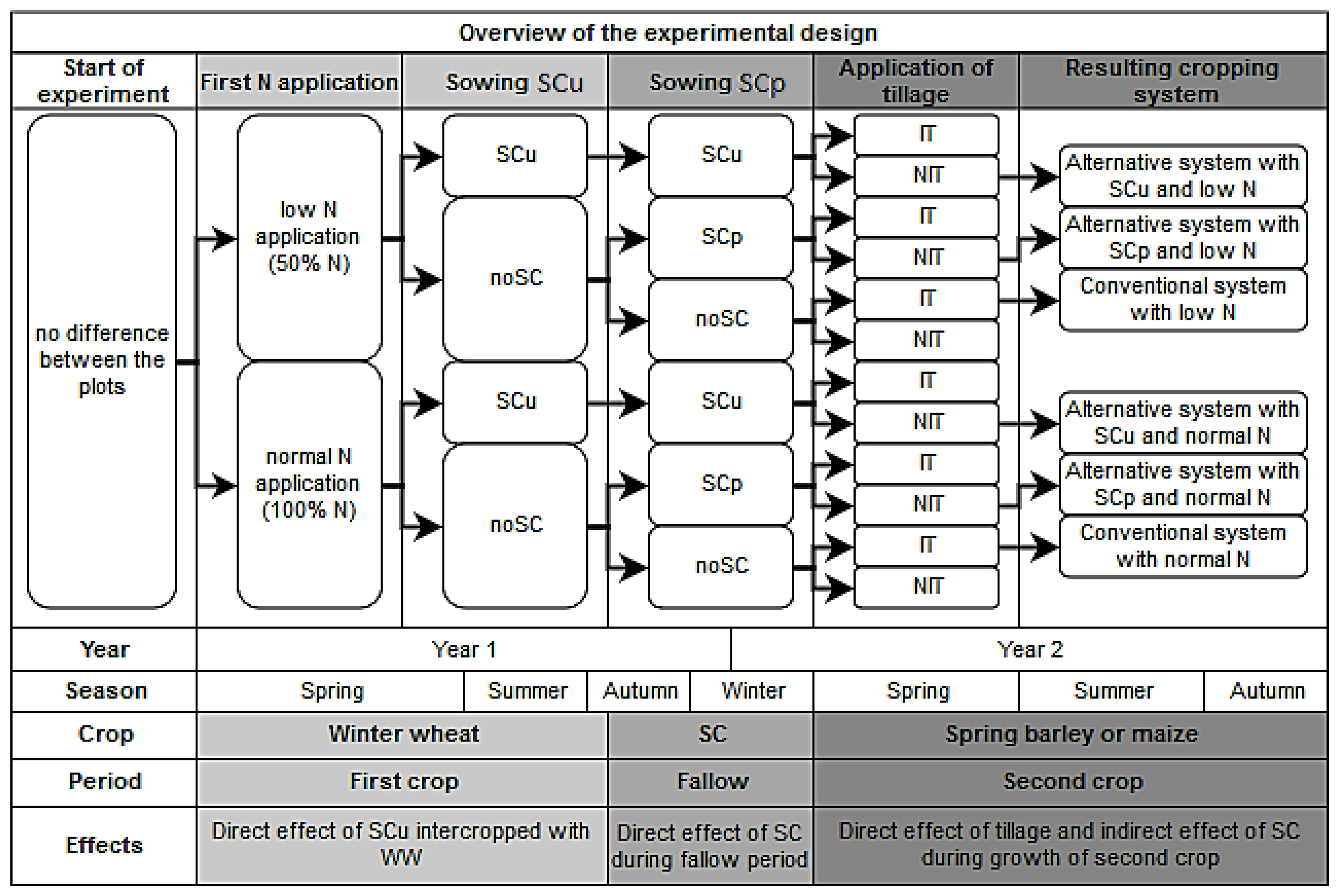
2.1. Experimental Design

Multi-environment experiments (MEE) were conducted at six sites from northern and central Europe: Norway (NO), United Kingdom (UK), two sites in Germany (DE org. and DE conv. for the organically and conventionally managed site, respectively), Sweden (SWE), and Switzerland (CH). The six sites represent four different climate zones in Europe: Continental (DE, CH), Nemoral (SWE), Atlantic North (UK), and Boreal (NO) [45]. The MEEs had a split-plot (with only one N fertilization level) or a split-split-plot design (with two N fertilization levels). The effect of tillage was investigated in the main plots, SCs in the sub-plots, and N fertilization in the sub-sub-plots (except in NO: N fertilization in sub-plots and SCs in sub-sub-plots). The plot size varied depending on the site between 48 m² to 162 m². The N fertilization level was included at four out of six sites (DE conv., SWE, NO, and CH) and had two levels, application of 100% or 50% of the locally recommended N dose (SWE and CH (Maize): 90 or 45 kg N ha−1, NO: 100 or 50 kg N ha−1, CH (wheat): 140 or 70 kg N ha−1, DE conv.: 200 or 100 kg N ha−1; soil nitrogen levels were not tested prior to the experiments). The tillage factor consisted of two levels, inversion tillage by mouldboard ploughing (IT) or non-inversion tillage (NIT), whereas the SC factor had three levels. SCs were either under-sown with the first crop winter wheat (SCu) or sown post-harvest (SCp) as cover crops. Control plots did not receive any SCs (no SC). Each experiment had four replicates (blocks). The design differed slightly among sites due to management-related reasons or because the experiments were designed to study further topics besides weeds (Table 1). Therefore, the different experiments must be seen as case studies.
Two rounds of MEEs were considered in this experiment. The first started in the autumn of 2012 and lasted until the autumn of 2014 (MEE1) and the repeats (MEE2) were started one year later (an overview and timeline of MEEs are given in Figure 1). The MEEs were ploughed and harrowed before starting the experiment by sowing winter wheat (WW, Triticum aestivum) in autumn of the first year. SCu were sown together with winter wheat in autumn (DE and CH) or under-sown into winter wheat in spring (NO, SWE, and UK). SCp were established after winter wheat harvest. The SCu and SCp species used for the experiments are listed in Table 2. The seeding dates and seeding density for each site can be seen in the Table S1. The SCs were terminated by tillage or herbicide use before the subsequent crop was sown in spring in year two at all sites except in SWE, where SCs in the IT treatment were incorporated before the soil was frozen in late autumn due to unsuitable conditions for spring ploughing. The main crop established in year two was spring barley (SB, Hordeum vulgare) in UK and NO, and maize (M, Zea mays) at the other sites. Tillage to establish the second main crop in year two was performed with the tillage sowing combination machine called “Eco-dyn” designed by Friedrich Wenz GmbH in the NIT system, (except for SWE, see Table 1) and by mouldboard ploughing to a depth of 22–30 cm with additional seedbed preparation (e.g., disking) in the IT system. Thus, the experiment was divided in three experimental periods (Figure 1). The period first crop ranged from sowing SCu until harvest of the first main crop (winter wheat), the period fallow ranged from the harvest of the first main crop (winter wheat) until sowing the second main crop (maize or spring barley), and the period second crop lasted throughout the growth of the second main crop. The N fertilization factor was applied in both winter wheat and the subsequent main crop. The SCs did not receive any fertilization. Further information on weed control measures and soil conditions at different sites are outlined in Table 1.

2.2. Data Collection

Weed abundance was defined as the combination of three different parameters: (i) weed ground coverage, (ii) weed biomass, and (iii) weed density. Weed ground coverage was defined as the percentage of ground that was covered by weeds. It was assessed visually over the whole plot except for the CH site where it was assessed in two 1 m² squares per plot (size: 48 m²). In addition to total weed coverage, the cover of the dominant weed species was also estimated (data not shown). Weed density and aboveground weed biomass per species were assessed in four randomly placed quadrats (quadrat area ranged from 0.125 m2 to 1.00 m2 depending on site and date) per plot each year. Weed biomass was sampled by cutting all plant biomass 3−5 cm above the soil surface. Biomass was separated by species before drying to determine dry weight. Density and biomass data were converted to plants m−2 or g m−2 before statistical analysis. In general, weed coverage was measured the most often, usually once during the growth phase and once at harvest during the main crops and during the growth of SCs or at least in spring in the fallow period. Weed biomass and density were measured less often, primarily once before the harvest of the main crops and once in spring at the end of the fallow period. A detailed list with the assessment dates of each site can be found in the Table S2).
The site-specific inherent weed pressure was determined by calculating an average over all treatments for each weed assessment (coverage, biomass, and density), site, MEE, and period (Figure 1; first crop, fallow, and second crop). The inherent weed pressure reflects the general level of weed infestation and was used as a moderator in the meta-analyses. To analyze the weed species composition, a list of all species and their appearance at the different experimental sites was compiled. For each site, the dominant weed species of each period were determined by sorting the weed species by their average of ground coverage over all treatments (Table S3).

2.3. Statistic Analysis

Before analysis, all weed assessment data for each site and each MEE round were sorted into the three experimental periods (first crop, fallow, and second crop (Figure 1)). The datasets were checked for homogeneity of variance and normality visually by residual vs. fitted plot and normal Q-Q plot. Within these datasets, the different assessments of weed abundance (coverage, biomass, and density) were analyzed separately using a mixed linear model. The three factors (tillage, SC, and N (if applied)) and their interactions were analyzed as fixed effects, and block effects and its interaction with main plots and subplots (N or SC depending on site) as random effects, according to the split-plot or split-split-plot design of the experiment. The analysis was first run with SCs divided into species and then grouped into SCp or SCu.
In all cases where the weed assessments were carried out more than once during an experimental period, a repeated measurement approach was used, with an assessment date as an additional fixed effect using the unstructured covariance structure. The “mixed” package in SAS 9.4 (SAS Institute Inc., Cary, NC, USA) was used for repeated measure analyses, and the “glimmix” package for non-repeated analyses. Post-hoc tests were performed using Tukey–Kramer adjustments. The estimated means and their standard deviations were taken from the mixed linear models to form a data set for each experimental period.
The meta-analyses were carried out using random-effects models with a restricted maximum-likelihood estimator (REML) for the residual heterogeneity using the metafor package in R as described by Viechtbauer [46]. The standardized mean difference (SMD) between groups and its 95% confidence interval (CI) was used to compare the effects of different treatments. Using SMD made it possible to compare the different types of weed assessments and to calculate an effect size over all three assessments. The resulting effect sizes were interpreted by using the modified Cohens rule of thumb suggested by Sawilowsky [47]: ≥0.01 very small, ≥0.2 small, ≥0.5 medium, ≥0.8 very large, ≥1.2 very large, and ≥2.0 huge. For easier interpretation, the effect sizes for weed coverage, biomass, and density were also calculated as mean differences (MD) to get the effect size in the original unit of %-ground coverage, g m−2 or plants m−2.
To determine the extent of heterogeneity, the I² parameter was used, as suggested by Higgins and Thompson [48]. The I² parameter estimates the proportion of the total variability in the effect size estimates that is due to heterogeneity. If the lower bound of the 95%-confidence interval (CI) were zero, the effect is assumed to be homogeneous; otherwise, the estimate for I² is used as a measure for the heterogeneity. The CI of the I² parameter was calculated by the confint command in the metafor package in R. In the case of heterogeneity, moderator variables were added to the meta-analyses. The following categorical moderator variables were analyzed separately for each comparison: weed assessment type, site, management (organic or conventional), MEE-round (MEE1 or MEE2), second crop species, and climate region after Jongman et al. [45]. The inherent weed pressure level was analyzed as a numeric moderator variable. The R² parameter was used to determine the amount of heterogeneity the moderator variables included in the model accounted for. An omnibus test was conducted to see if the moderator variable had a significant influence (p-value of the QM-test < 0.05; [46]). Moderators were only tested on SMD.
To find the combination of tillage and SCs with the best weed control, all possible combinations were tested against the combination of IT and no SC cultivation, which was used to represent a reference system, in the second crop period. For each comparison, a meta-analysis for the whole dataset, and the three subsets (coverage, biomass and density) was calculated.
To analyze the effect of type of management (organic vs. conventional), MEE round and site on the inherent weed pressure linear models were used and calculated using the lme4 package in R. The data were divided by experimental period and weed assessment. For each dataset, a separate one-way ANOVA was performed.

3. Results

3.1. Weed Abundance and Species Composition

The inherent weed pressure was relatively high in NO and UK and relatively low in DE conv. and CH over all experimental periods and weed assessments. Furthermore, there was a tendency that the organically managed experiments had a higher inherent weed pressure (Figure S1). Overall, the mean inherent weed pressure was relatively low in the first crop period with 9% weed ground coverage but increased in the fallow period (30% weed ground coverage) and second crop period (22% weed ground coverage).
The only weed species present at all sites was Cirsium arvense, although it was not the most dominant weed at all sites. The most common dominant weed species were mainly dicots like Stellaria media, Chenopodium album, Rumex spp., and Tripleurospermum inodorum. The most common dominant monocot was Elymus repens. However, while the dominant species differed between sites, the weed species found are commonly associated with arable land [20,49,50,51]. The weed species composition at the UK experimental sites differed from the other sites: monocots were more prevalent, and the weed species were more closely associated with grasslands (a detailed list with all weed species found and the most dominant weed species can be found in Tables S3 and S4).

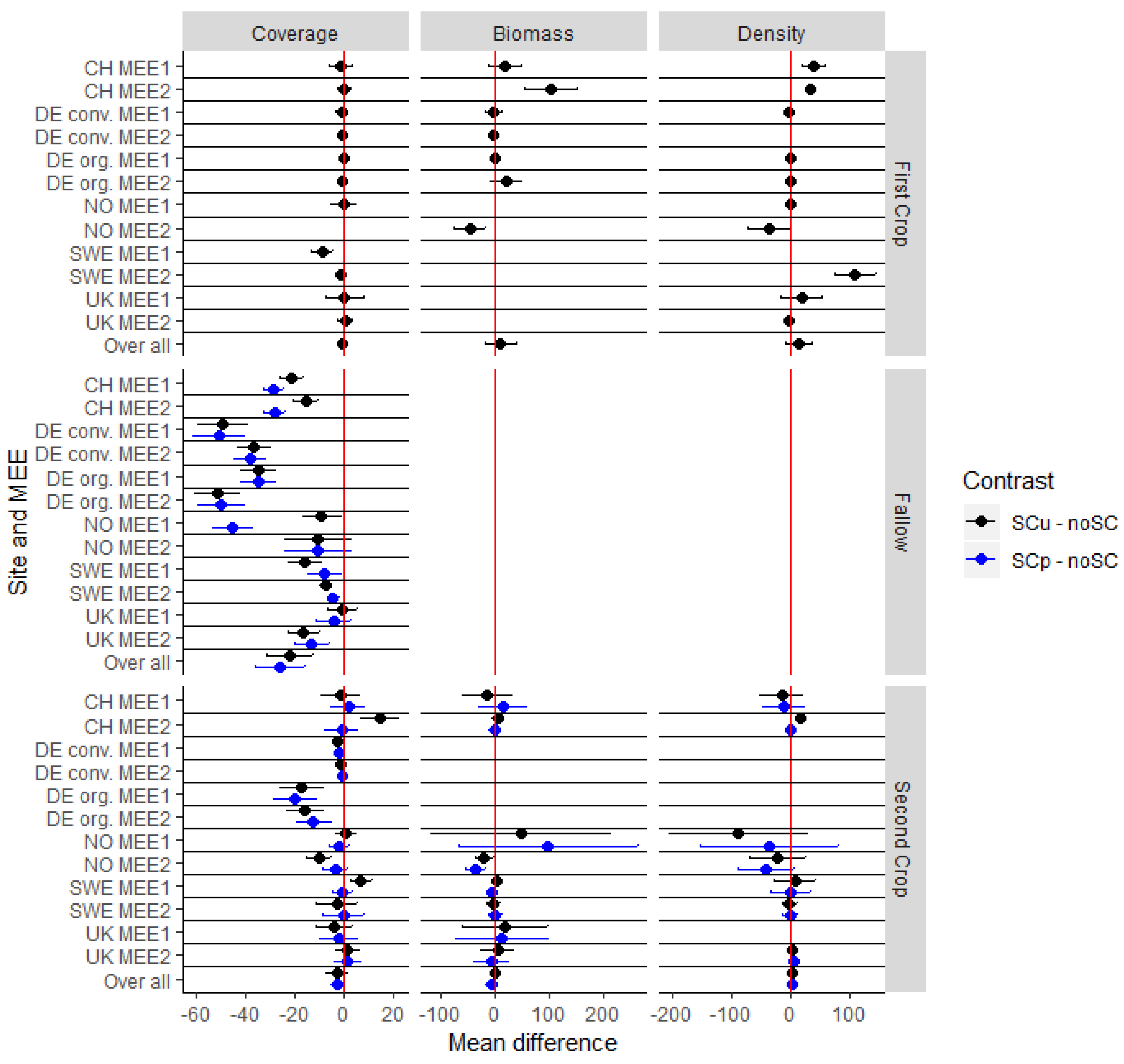
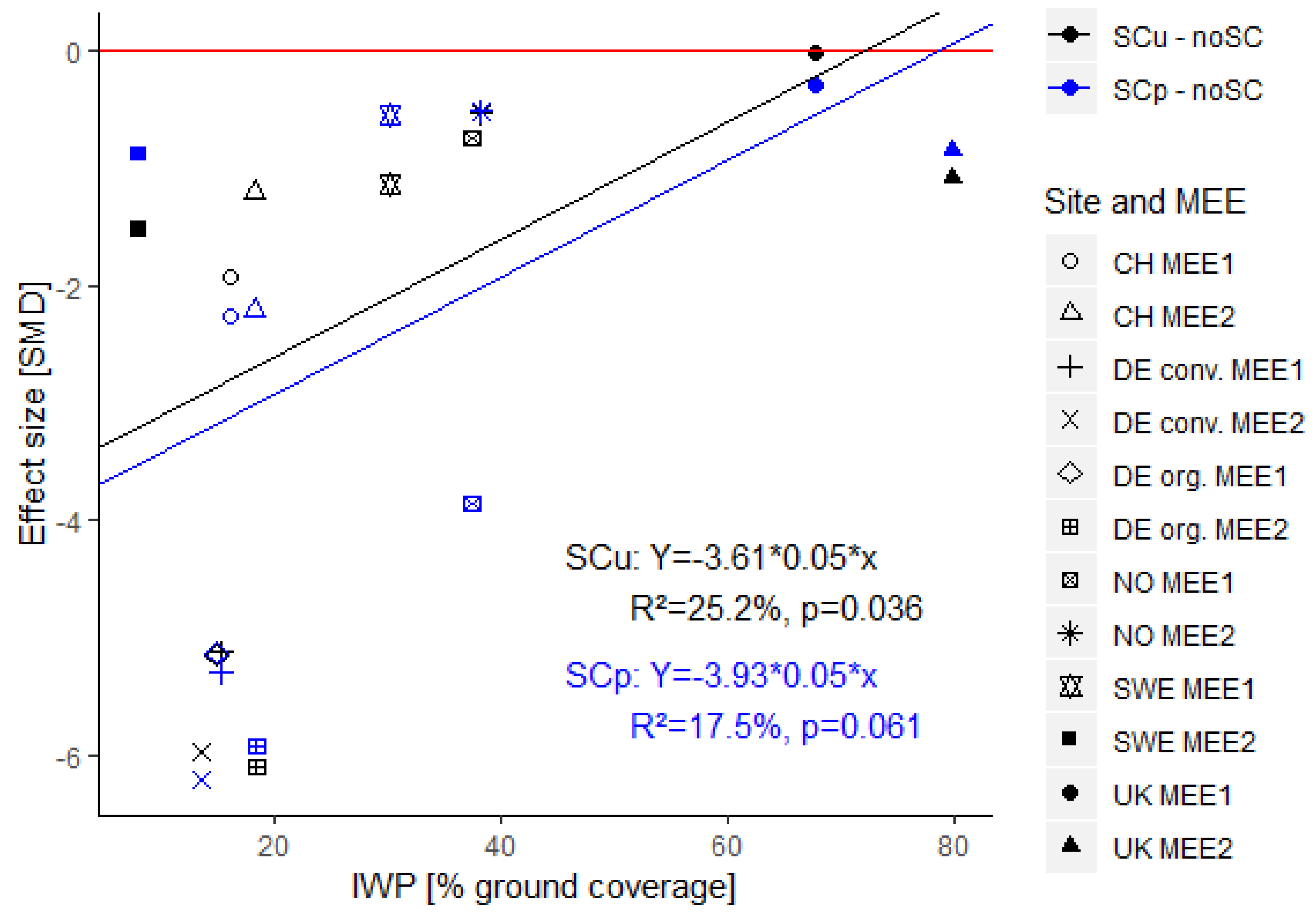
3.2. Effect of Subsidiary Crops on the Weed Abundance

3.2.1. Weed Control

The effects of SCs on the weed abundance differed greatly (I² above 60%) between weed assessment type, experimental periods, site, management type (organic or conventional) and inherent weed pressure (Table 3, Figure 2). The SCs had little influence on weed biomass and, even less on weed density, but there was high heterogeneity in the data (Figure 2). In contrast, both SCu and SCp were able to reduce the weed coverage by up to 26 percentage points during the fallow period, compared to no SCs (Table 3). There was little effect of SCs in the first crop and second crop periods.
SCs reduced weed coverage the most at the German sites, especially DE org. (effect sizes up to -5 in the fallow period; Figure 2). In contrast, SCs, especially SCu, had almost no effect or even increased weed abundance at UK in the first main crops and at CH in the first and second main crop.
In general, the SCs suppressed weeds more at organically managed sites than at conventional ones. This was especially pronounced in the second crop period where the organic sites showed significant negative effect sizes even though the moderation by type of management was not strong (QM-p > 0.05; R² < 10%).
With an increase in inherent weed pressure, the weed control by SCs decreased throughout the experimental periods. This effect was most pronounced in the fallow period (R² up to 25%; Figure 3).

3.2.2. Differences between Subsidiary Crop Sowing Time (SCu and SCp) and Species

There were very few differences between the use of SCu and SCp. Only in the fallow period, SCu had a better weed control (slightly more negative effect size, Figure 2) in the northern climates (NO MEE2 /SWE both MEEs). In contrast, SCp had a clear advantage over SCu in CH.
There were only a few significant differences between different SCu and SCp species (Table S6). As SCu, the mixtures of legume and non-legume species were in most cases better at reducing weeds abundance than their pure stands (Table S6). Further, subterranean clover had a better weed control effect than white clover at DE org. As SCp, hairy vetch had a higher weed control effect than oilseed radish in DE org. and CH.

3.3. Effect of N Fertilization on the Weed Abundance

No significant effect of N fertilization on the weed abundance was detected, in either the meta-analysis over all sites and MEE-rounds, or at any site and MEE-round alone in any of the experimental periods. Further, there was no substantial heterogeneity of the data detected. Therefore, no moderators were tested. The three-way interaction of N fertilization with the other two factors (SC and tillage) also did not show any other effects than the two-way interaction of the other factors alone.

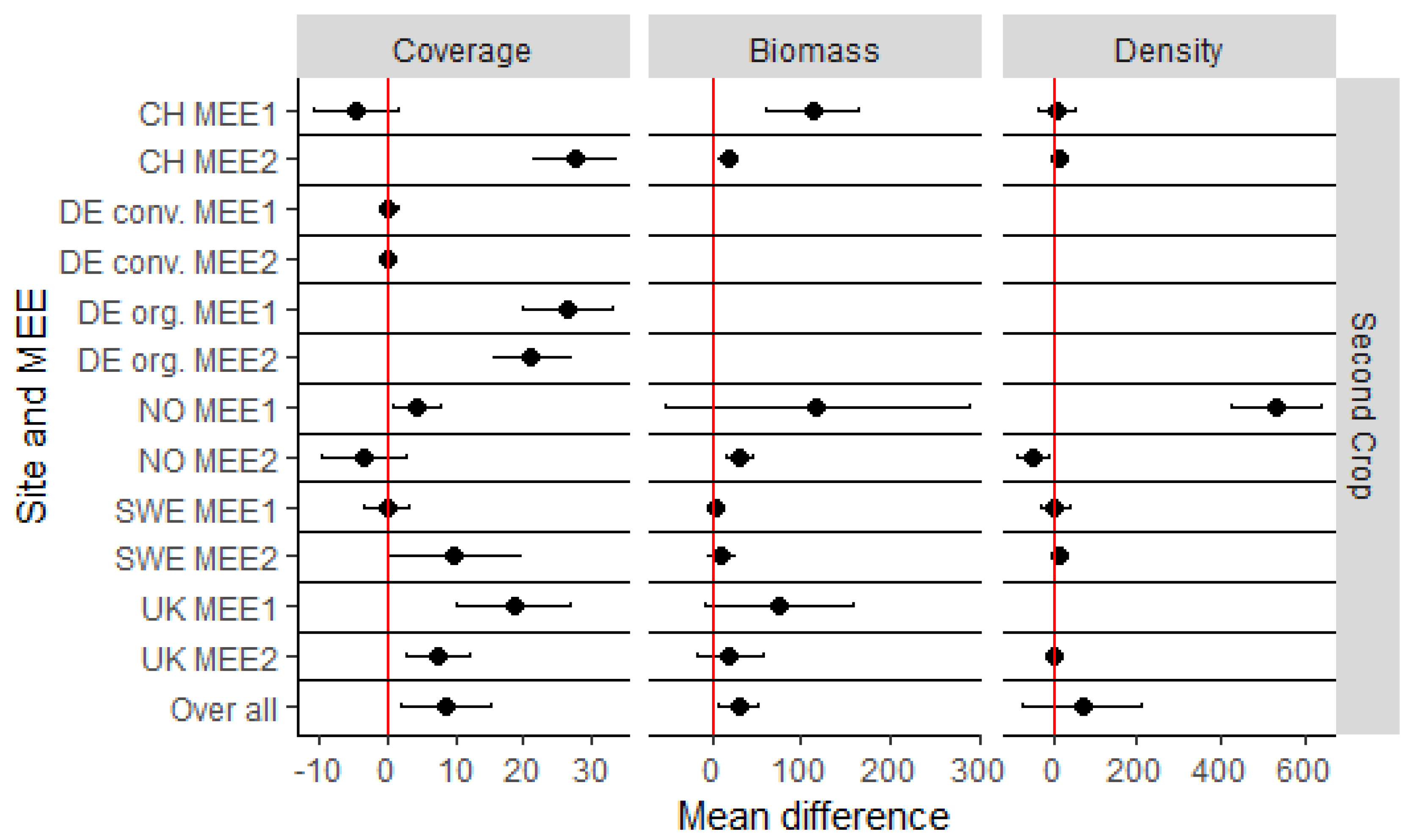
3.4. Effect of Tillage on the Weed Abundance

The tillage factor was only applied before the second crop and therefore its effect can only be analyzed in that period. Overall IT resulted in moderately less weed coverage and biomass than NIT (SMD > 0.5; p < 0.001), while there was no significant difference in weed density between the treatments (Table 3). The large heterogeneity within the weed coverage and density were primarily due to differences between sites (R² = 66% overall assessments, Figure 4). DE org. had a particularly large effect size in favour of IT (SMD = 2.43), while DE conv. and SWE had little to no difference between the two treatments.
Management type explained some of the heterogeneity (R² = 11% for weed coverage), as IT, in particular, was a more effective weed control measure than NIT at organically farmed sites compared to conventional ones (conventional: SMD = 0.37, organic: SMD = 0.79 over all assessments).
The inherent weed pressure also moderated the effect of tillage (Table 3) although, the effect was less clear than for SCs. After removing outliers (NO MEE1 due to an extremely high weed pressure), the results show that a higher inherent weed pressure resulted in IT having a lesser advantage in regards to weed density, but a greater advantage in regards to weed coverage.

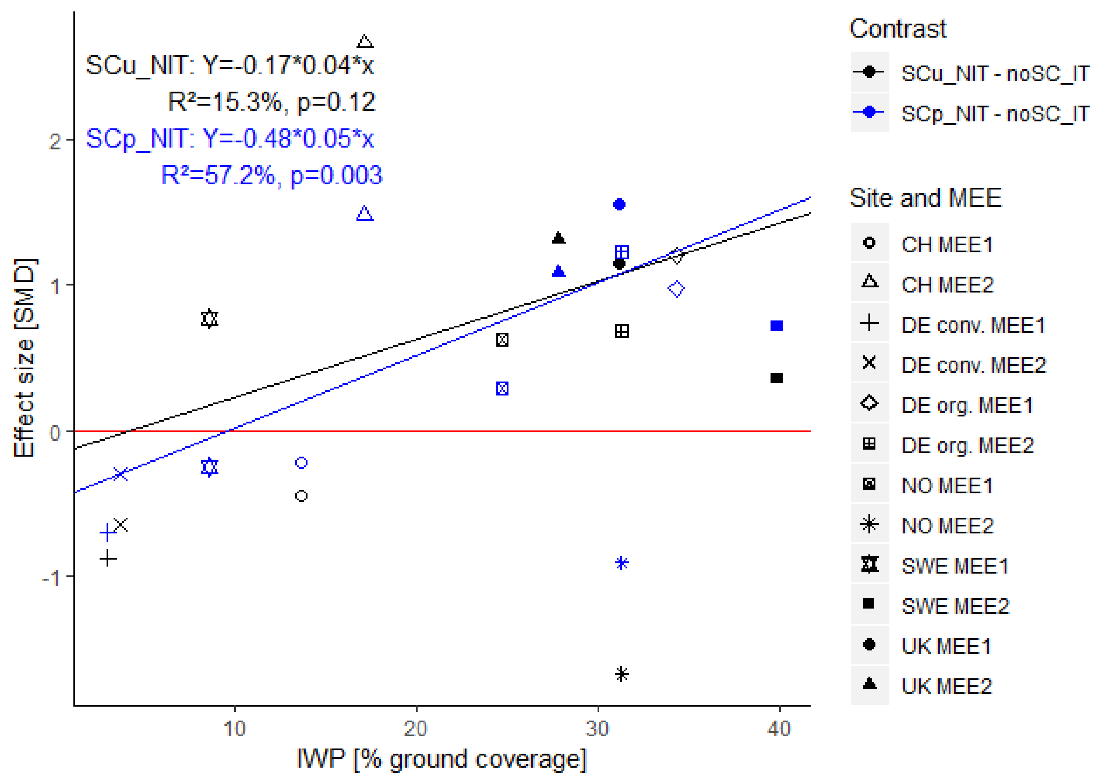
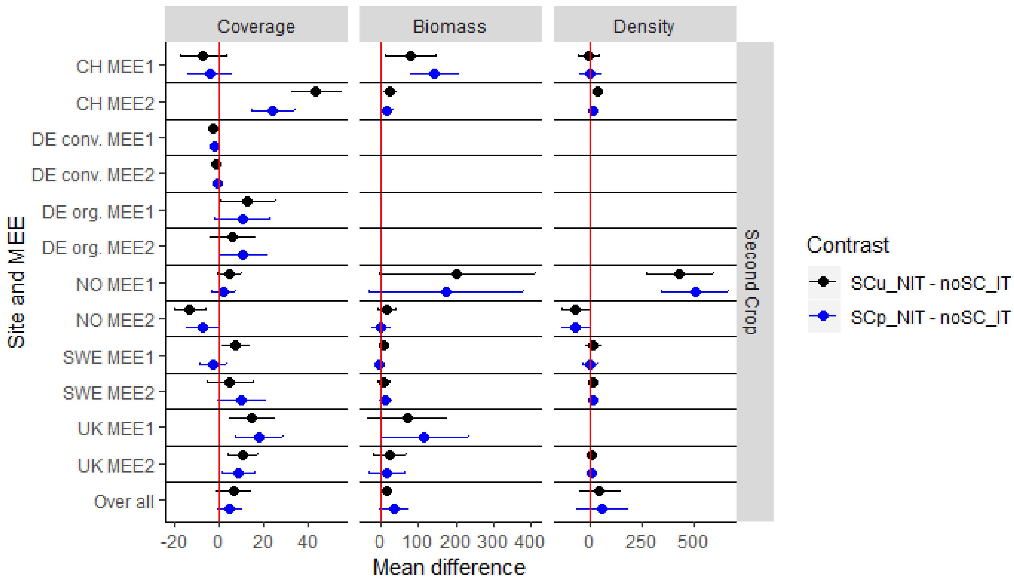
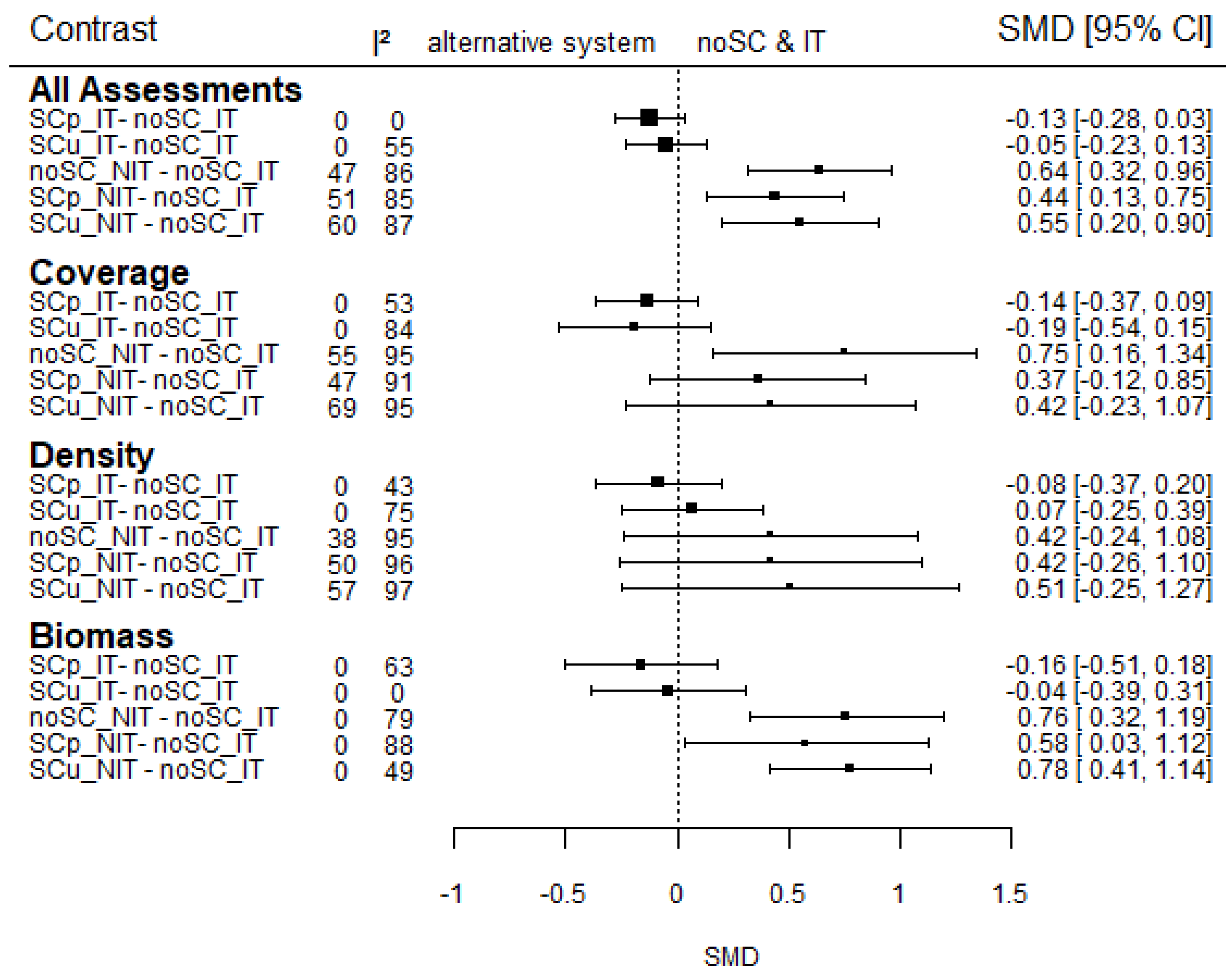
3.5. Effect of the Interaction between Subsidiary Crops and Tillage on the Weed Abundance

3.5.1. Non-Inversion Tillage and Subsidiary Crops vs. Ploughing System

Since N fertilization did not have any effect on weed abundance or the performance of the other factors, it was decided to exclude it as a factor for the interaction analysis. Therefore, the focus was on the interaction of the two remaining factors—tillage intensity and SCs—and their effect and weed abundance in the second crop period.
In general, the alternative systems (NIT combined with SCp or SCu) resulted in a larger weed biomass in the second crop, regardless of SC type used, than in the reference system (IT without a SC; Table 3). The SCu-based alternative system showed more heterogeneity within the data than the SCp-based alternative system (Table 3). Inherent weed pressure explained some of the heterogeneity, with the alternative system becoming less efficient compared to the reference system the higher the inherent weed pressure (Figure 5). (NO MEE2 data were removed as an outlier due to very different weeding regimes in SCs compared to no SC treatments.)
Only a small amount of the heterogeneity could be explained by moderators due to the high variation within experimental sites (e.g., NO and CH Figure 6). However, site was still able to explain some of the heterogeneity. At DE conv., weed abundance was somewhat lower in the alternative than in the reference system (Figure 6). The opposite can be seen in DE org., UK and SWE (for SCu_NIT only).

3.5.2. Combination of Tillage and Subsidiary Crop with Highest Weed Control

To test which system (excluding N fertilization) resulted in the best weed control in the second crop, all different combinations were tested against the reference system (no use of SCs and IT). There was a recurring pattern, particular over all assessments, that systems based on IT with the cultivation of SCs (SCp_IT and SCu_IT) had the smallest weed abundance, with an exception of SCu_IT for weed density, but the differences were never significant compared to the reference system (Figure 7). The systems based on NIT had a higher weed abundance, which was significant for the biomass assessment and overall assessments, and showed high heterogeneity particularly for the coverage and biomass assessments.

4. Discussion

The aim of the study was to investigate whether an NIT-based cropping system that includes SCs and reduced N-fertilization can effectively control weeds in the year of establishment and in the subsequent crop. Therefore, the effects of SCs, tillage, and N fertilization and their interactions on weed abundance were investigated during three growing phases [first crop, fallow (this includes the time when SCs alone were growing between main crops), and second crop period] in six case studies throughout northern and central Europe during the transition time to NIT. We found that during this initial phase weed abundance was lower in IT than in NIT and with SCs than without. The effect of SCs was smaller than the effect of tillage system. We did not find any significant effect of N fertilization on weed abundance. Thus, the combination of NIT and SCs resulted in higher weed abundance than the reference system approach of IT and no SC. The factors that had the greatest influence on weed control efficacy were site and inherent weed pressure, but management type (organic/conventional) and climate zone also had some influence.
In the interpretation of the data, it needs to be noted, however, that this study is based on two-year rotation experiments. It has been shown that the effects of reduced tillage intensity and SCs on weeds and soil properties, especially soil organic matter, need time to build up [7,14,52]. For SCs the effect of reduced weed seed production [53,54] and increasing weed seed predation [30], in particular, will most likely only have effects in the long-term. Nevertheless, in a parallel experiment conducted within the same time period in Germany, using compost applications in addition to SCs, the combination of SCs with compost was able to maintain the seed bank in NIT at similar levels to IT during the transition period [55]. This and the findings of the presented study are relevant for the transition period and may help in choosing the best conditions to successfully transition to NIT, but the data cannot be used to infer the long-term differences between NIT and IT.
The first hypothesis, that growing SCs during the first crop and/or fallow period will result in lower weed abundance during concurrent and subsequently growing phases (first crop, fallow, and second crop period), can only be partially supported by the results of this study. SCs generally reduced the weed coverage during the fallow period, but only to a small extent in the other periods. This supports the common understanding in the literature that the cultivation of SCs can lead to a reduced weed abundance during their growth [26,54,56], but has a small effect on the success of the main crops [57,58]. This study is based on six sites (and five countries), which enabled us to obtain more general conclusions compared to those earlier studies which were performed at one location each.
It is noteworthy that the SCs reduced weed coverage, but not weed biomass or density. This contrast with the results of Radicetti et al. [59] who found a significant decrease in weed biomass due to SCu cultivation in the first crop period in temperate and Mediterranean climate zones in Europe. One reason could be that coverage assesses the whole plot and is, therefore, less sensitive to patchy weed abundance. Another reason could be that the SCs actually had small effect on the weed abundance, but they made it more difficult to measure the crop coverage accurately. More objective measures (e.g., weed biomass) are less sensitive to such errors than subjective visual estimates. Another reason for the lack of an SC effect on weed biomass and density as found in the analyses is that these were not measured when SCs had their greatest effect according to the coverage measurements—during the fallow period and at the German sites.
The strong influence of site on SC weed suppression efficacy can be partially explained by differences in climate between sites and also through nutrient effects in the organic system in DE org. SCp in sites with colder climates tended to have a lower weed suppression in the fallow period than SCp grown in warmer climates. The growing period in autumn in northern regions is too short for an SCs sown after harvest to establish well enough to be a good competitor towards weeds [26], potentially making under-sowing more suitable. The advantage of SCp over SCu in the warmer climates, on the other hand, is most likely not because the SCp were more competitive, but rather that additional tillage was performed while or prior to sowing the SCp in autumn.
Differences in management between sites may also explain in part why the site had such a large influence on SC efficacy. For example, sites with wide-row spacing in the first crop period (DE org. and DE conv.) also had strong weed suppression by SCs. At CH, even though herbicides were used in the no SC control and not in the SCu in the first crop period, SC still achieved a similar weed coverage. Showing the potential of reducing herbicides treatments through SC cultivation.
The moderators included in this study were not able to explain the whole heterogeneity within the data. Other factors such as traits of the SC species, the local weed community, and other abiotic factors might explain some of the remaining variations. Uchino et al. [60] describe the effect of different characteristics of SCs on weed control efficiency. They concluded that the coverage and biomass of an SC are the crucial characteristics when it comes to weed control. Others have argued that the relationship is more complex, and that additional traits also determine the effectiveness of the control, which vary from species to species [28,61,62].
Type of species used as an SCu or SCp caused little differences in this study. However, the use of mixtures of legumes with grass or Brassicaceae species often had an advantage over pure stands of the same legume species, similarly to Baraibar et al. [54]. Mixtures can occupy more ecological niches than pure stands and combine different modes of competition, for example by evenly reducing both below and aboveground weed biomass instead of primarily reducing just one [61,63]. In case of the failure of one species component, the other species can compensate [64]. Moreover, the relatively slow growth rate of legumes, such as clover species, under conditions with high amounts of available N can be compensated by higher growth rates of companion crops [54,65]. Further, hairy vetch as a legume SCp had a better weed control than non-legume SCp oilseed radish. Since legumes are self-sufficient regarding N fertilization, and no N was added before sowing SCp, this might have led to an advantage for the legume over the non-legume species especially at the organically managed site in DE. However, the N input is a double-edged sword—fertilizing both succeeding crops and weeds [64,66,67]. Thus, it should be noted that there is no one-size-fits-all solution when it comes to deciding which species or variety of SCs results in the best weed control. The species and varieties should be picked according to site-specific needs. A decision support tool was created based on the data from the optimising subsidiary crop applications in rotations (OSCAR) trials to help farmers to choose appropriate SCs [68].
Over all of the experiments, the N fertilization level had no significant effect on weed abundance, while SCs generally had a smaller effect than using IT instead of NIT. Consequently, we must reject the second hypothesis—that weed abundance is lower in the first years of an NIT system compared to IT when using lower N fertilization and SCs (noSC_IT). The fact that N fertilization level did not have any significant effect on weed abundance or on the performance of the other factors indicates that N fertilization benefited the growth of all plants (SCs, main crop, and weeds) equally. This stands in contrast with most previous studies, which have found strong effects of N fertilization on different weed species like e.g., Amaranthus spinosus L. [38,40]. A likely explanation for this discrepancy is that most studies focus on specific weed species rather than the whole weed population. Thus, N fertilization might change the weed species composition rather than the total weed abundance [41]. Likewise, Swanton et al. [69] found that N fertilization did not influence weed density when investigated in combination with SCs and tillage intensity treatments.
The results of the study suggest that using IT instead of NIT had a stronger influence on the weed abundance in the second crop than SCs. Similarly, Bàrberi and Mazzoncini [20] found that weed density was only influenced by tillage and herbicide management system and not by SCs (in this case SCp) in the second crop in a short-term period. Contrasting, in a long-term perspective SCs had a weed reducing effect [21]. However, since the weed control effect of SCs (as discussed above) depended greatly on the site/management, weed assessment type, and inherent weed pressure, so did the weed abundance in the SC_NIT system. As a result, noSC_IT only had significantly lower weed abundance than SC_NIT in half the experiments: CH, SWE MEE1, UK, and NO MEE1. The yields were not investigated in this study, however yield data for the first crop is presented and discussed in Radicetti et al. (2018) [59] and the data for the second crop is presented in the final report of the OSCAR project [70].
At some sites, management decisions had a clear impact on SC and tillage efficacy. For example, at CH herbicides were used in IT plots and hoeing in NIT plots, giving an advantage to the IT plots, which SCs could not compensate for. This can be contrasted to the two German sites that were sowing the SCs earlier and achieved good weed suppression so that SC_NIT did not have significantly more weed abundance than noSC_IT. However, herbicide use at DE conv. meant that the difference between SC_NIT and no SC_IT was smaller than at DE org., emphasizing the advantage of IT over NIT in the absence of herbicides [11]. Only one experiment, NO MEE2, showed less weed abundance in the SC_NIT treatment. However, this was likely due to the additional hoeing performed in the NIT plots rather than suppression by SCs. On the one hand, this supports the view that management factors such as tillage intensity and herbicides have larger effects on the weed abundance than SCs [26]. On the other hand, the potential of weed suppression by SCs, as seen at the German, Norwegian, and Swedish sites, could mean that fewer additional weed control measures are necessary to achieve a similar weed suppression as IT. Moreover, it shows the importance of optimizing SC management, e.g., sowing time and row-distance, in order to produce sufficient amount of SC biomass and ground coverage for weed suppression and to make SCs compatible with weed control measures less intense than IT [20,71]. A third factor that influenced the weed control effect of SCs in an NIT system was the inherent weed pressure at the sites. With increasing inherent weed pressure, the advantage of noSC_IT over SC_NIT increased. In general, the weed control by SCs decreased with increasing inherent weed pressure. A high weed pressure level seemingly gave the weeds a competitive advantage over the SCs. This effect was most pronounced in the fallow period but continued into the second crop period. Zasada et al. [72] also found that the use of SCp was only effective at low initial weed densities compared to high initial weed densities. This could mean that SCs are only a sufficient weed control measure if the inherent weed pressure is low, giving the SC a competitive advantage over the weeds. The reason for this competitive advantage could be a higher inter-competition between weeds and SCs compared to high intra-competition within the SCs at high weed pressure due to better or quicker establishment of the SCs. Further research on the relation of weed pressure and SC weed suppression will be needed to determine the cause of the competitive advantage of weeds at high weed pressure.
The moderation by inherent weed pressure was less clear for tillage than for SCs. There were opposing results depending on which weed assessment method was used—for weed density, an increase in inherent weed pressure decreased the advantage of IT over NIT but for weed coverage, the opposite was the case. However, it has to be noted, that not all sites had density measures and therefore the density assessment is not as representative as weed coverage. Further detailed studies on how the inherent weed pressure influences the effect of tillage might be needed to explain this contrast. Taking these two moderations by inherent weed pressure on the weed control by tillage and SCs together, they resulted in a higher advantage of the reference system at high weed pressure.
The best weed control was achieved by the combination of IT and SCs. Therefore, a recommendation would be to implement an NIT system with SCs on fields with low weed pressure, but to use an IT-based system with the cultivation of SCs as an effective weed control agent in fields with high inherent weed pressure levels before implementing an NIT system. This would incorporate the environmental benefits of SCs with good weed control and might reduce the need for herbicides. In fields with lower inherent weed pressure, SC alone can be sufficient to reduce weed abundance, especially when combined with additional measures, such as compost applications [55] and can, therefore, be used to convert to NIT to maximize the ecosystem services of the system in the long run.

5. Conclusions

Across six different sites in Northern and Central Europe subsidiary crops, sown after harvest of the main crops reduced weed coverage more than under-sown subsidiary crops. The effect varied greatly from site to site, showing the potential of subsidiary crops as a weed control measure, but also the importance of adapting management to local conditions. For the transition phase to NIT, which was investigated in this study, the subsidiary crops was only able to compensate for the reduced weed control by NIT in half of the case studies where overall weed pressure was not excessive. Therefore, a transition to a system based on reduced tillage should primarily be recommended when the weed pressure is low (<15% weed ground coverage), while under high weed pressure (>15% weed ground coverage), IT in combination with subsidiary crops and/or herbicides may be necessary to achieve a low weed pressure before conversion to reduced tillage. Fertilizer management did not have any effect on the overall weed abundance. The weed control efficacy was highly influenced by site, more specifically the additional chemical and mechanical weed control measures used at the sites, cultivation management, and the level of inherent weed pressure.

Supplementary Materials

The following are available online at https://www.mdpi.com/2073-4395/9/9/495/s1, Figure S1: Inherent weed pressure measured as the average weed coverage (top left), weed biomass (top right), and density (bottom left) over all treatments, Table S2: All assessment dates and stages at the six sites and both MEE round sorted into the three approaches, Table S3: Three dominant species for each site, MEE-round and experimental phase. The order is determined by ground cover. For DE org. four species are picked in the first crop period since they tied, Table S4: List of weed species found at the different sites. “freq” states the number of sites the weed species is found. EPPO-Code according to EPPO (2018)., Table S5: Standardized mean differences (SMD; eff.) and the 95% confidence interval (lower border Cl lb; upper border Cl ub) for all contrasts, experimental periods (first crop, fallow and second crop) and weed assessment types (ground coverage, biomass, and density), Table S6: List showing differences between the species within the under-sown subsidiary crops (SCu) and the post-harvest sown subsidiary crops (SCp) group for every site, MEE-round, and weed assessment in each experimental period, 2: Dataset of the study: “Under low weed pressure subsidiary crops confer sufficient weed control in reduced tillage systems. A case study across northern and central Europe.” By Reimer et al.

Author Contributions

Conceptualization, G.B., S.W., R.W., J.P.B., M.G.A.v.d.H., K.M., M.R.F., and L.O.B.; formal analysis, M.R.; funding acquisition, M.R.F.; investigation, G.B., S.W., R.W., J.P.B., K.M., and L.O.B.; methodology, M.R., B.R., G.B., S.W., R.W., J.P.B., M.G.A.v.d.H., K.M., M.R.F., and L.O.B.; project administration, M.R.F.; supervision, B.R. and L.O.B.; visualization, M.R.; writing—original draft, M.R.; writing—review and editing, B.R., G.B., S.W., R.W., J.P.B., M.G.A.v.d.H., K.M., M.R.F., and L.O.B.

Funding

This study was based on data acquired by the OSCAR “Optimising Subsidiary Crop Applications in Rotations” project, which was financed by the European Union FP7 Project (Grant agreement ID: 289277).

Acknowledgments

The authors would like to thank the editor and two anonymous reviewers for their comments during the review process. The author would also like to thank the European Union FP7 Project for financing the project.

Conflicts of Interest

The authors declare no conflict of interest.

References

  1. Krauss, M.; Berner, A.; Burger, D.; Wiemken, A.; Niggli, U.; Mäder, P. Reduced tillage in temperate organic farming: Implications for crop management and forage production. Soil Use Manag. 2010, 26, 12–20. [Google Scholar] [CrossRef]
  2. Scopel, E.; Triomphe, B.; Affholder, F.; Da Silva, F.A.M.E.; Corbeels, M.; Xavier, J.H.V.; Lahmar, R.; Recous, S.; Bernoux, M.; Blanchart, E.; et al. Conservation agriculture cropping systems in temperate and tropical conditions, performances and impacts. A review. Agron. Sustain. Dev. 2013, 33, 113–130. [Google Scholar] [CrossRef]
  3. Chan, K.Y. An overview of some tillage impacts on earthworm population abundance and diversity—Implications for functioning in soils. Soil Tillage Res. 2000, 57, 179–191. [Google Scholar] [CrossRef]
  4. Pelosi, C.; Pey, B.; Hedde, M.; Caro, G.; Capowiez, Y.; Guernion, M.; Peigné, J.; Piron, D.; Bertrand, M.; Cluzeau, D. Reducing tillage in cultivated fields increases earthworm functional diversity. Appl. Soil Ecol. 2014, 83, 79–87. [Google Scholar] [CrossRef]
  5. Holland, J.M. The environmental consequences of adopting conservation tillage in Europe: Reviewing the evidence. Agric. Ecosyst. Environ. 2004, 103, 1–25. [Google Scholar] [CrossRef]
  6. Govaerts, B.; Verhulst, N.; Castellanos-Navarrete, A.; Sayre, K.D.; Dixon, J.; Dendooven, L. Conservation agriculture and soil carbon sequestration: Between myth and farmer reality. Crit. Rev. Plant Sci. 2009, 28, 97–122. [Google Scholar] [CrossRef]
  7. Haddaway, N.R.; Hedlund, K.; Jackson, L.E.; Kätterer, T.; Lugato, E.; Thomsen, I.K.; Jørgensen, H.B.; Isberg, P.E. How does Tillage Intensity Affect Soil Organic Carbon? A Systematic Review; BioMed Central: London, UK, 2017. [Google Scholar]
  8. Seitz, S.; Goebes, P.; Puerta, V.L.; Pereira, E.I.P.; Wittwer, R.; Six, J.; van der Heijden, M.G.A.; Scholten, T. Conservation tillage and organic farming reduce soil erosion. Agron. Sustain. Dev. 2019, 39, 4. [Google Scholar] [CrossRef]
  9. Montgomery, D.R. Soil erosion and agricultural sustainability. Proc. Natl. Acad. Sci. USA 2007, 104, 13268–13272. [Google Scholar] [CrossRef] [Green Version]
  10. Baral, K.R. Review: Weed management in organic farming through conservation agriculture practive. J. Agric. Environ. 2012, 13, 60–66. [Google Scholar] [CrossRef]
  11. Peigné, J.; Ball, B.C.; Roger-Estrade, J.; David, C. Is conservation tillage suitable for organic farming? A review. Soil Use Manag. 2007, 23, 129–144. [Google Scholar] [CrossRef]
  12. Vakali, C.; Zaller, J.G.; Köpke, U. Reduced tillage effects on soil properties and growth of cereals and associated weeds under organic farming. Soil Tillage Res. 2011, 111, 133–141. [Google Scholar] [CrossRef]
  13. Hǻkansson, S. Weeds and Weed Management on Arable Land: An Ecological Approach; Hakansson, S., Ed.; CABI: Wallingford, UK, 2003. [Google Scholar]
  14. Semb Tørresen, K.; Skuterud, R.; Trandsæther, H.J.; Bredesen Hagemo, M. Long-term experiments with reduced tillage in spring cereals. I. Effects on weed flora, weed seedbank and grain yield. Crop Prot. 2003, 22, 185–200. [Google Scholar] [CrossRef]
  15. Peigné, J.; Casagrande, M.; Payet, V.; David, C.; Sans, F.X.; Blanco-Moreno, J.M.; Cooper, J.; Gascoyne, K.; Antichi, D.; Bàrberi, P.; et al. How organic farmers practice conservation agriculture in Europe. Renew. Agric. Food Syst. 2016, 31, 72–85. [Google Scholar] [CrossRef]
  16. Sans, F.X.; Berner, A.; Armengot, L.; Mäder, P. Tillage effects on weed communities in an organic winter wheat-sunflower-spelt cropping sequence. Weed Res. 2011, 51, 413–421. [Google Scholar] [CrossRef]
  17. Barberi, P.; Aendekerk, R.; Antichi, D.; Armengot, L.; Berner, A.; Bigongiali, F.; Blanco-Moreno, J.M.; Carlesi, S.; Celette, F.; Chamorro, L.; et al. Reduced tillage and cover crops in organic arable systems preserve weed diversity without jeopardising crop yield. Build. Org. Bridges 2014, 3, 765–767. [Google Scholar]
  18. Büchi, L.; Wendling, M.; Amossé, C.; Necpalova, M.; Charles, R. Importance of cover crops in alleviating negative effects of reduced soil tillage and promoting soil fertility in a winter wheat cropping system. Agric. Ecosyst. Environ. 2018, 256, 92–104. [Google Scholar] [CrossRef]
  19. Swanton, C.J.; Weise, S.F. Integrated Weed Management: The Rationale and Approach. Weed Technol. 1991, 5, 657–663. [Google Scholar] [CrossRef]
  20. Bàrberi, P.; Mazzoncini, M. Changes in weed community composition as influenced by cover crop and management system in continuous corn. Weed Sci. 2001, 49, 491–499. [Google Scholar] [CrossRef]
  21. Carlesi, S.; Antichi, D.; Bigongiali, F.; Mazzoncini, M.; Barberi, P. Long term effects of cover crops on weeds in Mediterranean low input arable management systems. In Proceedings of the 17th European Weed Research Society Symposium, Montpellier, France, 22–26 June 2015. [Google Scholar]
  22. Hartwig, N.L.; Ammon, H.U. Cover crops and living mulches. Weed Sci. 2002, 50, 688–699. [Google Scholar] [CrossRef]
  23. Thorup-Kristensen, K.; Magid, J.; Jensen, L.S. Catch crops and green manures as biological tools in nitrogen management in temperate zones. Adv. Agron. Vol. 2003, 79, 227–302. [Google Scholar]
  24. Bàrberi, P. Weed management in organic agriculture: Are we addressing the right issues? Weed Res. 2002, 42, 177–193. [Google Scholar] [CrossRef]
  25. Liebman, M.; Davis, A.S. Integration of soil, crop and weed management in low-external-input farming systems. Weed Res. 2000, 40, 27–47. [Google Scholar] [CrossRef] [Green Version]
  26. Teasdale, J.R.; Brandsaeter, L.O.; Calegari, A.; Skora Neto, F. Cover crops and weed management. In Non- Chemical Weed Management; Upadhyaya, M.K., Blackshaw, R.E., Eds.; CAB International: Vancouver, BC, Canada, 2007; pp. 49–64. [Google Scholar]
  27. Blackshaw, R.E.; Moyer, J.R.; Doram, R.C.; Boswell, A.L. Yellow sweetclover, green manure, and its residues effectively suppress weeds during fallow. Weed Sci. 2001, 49, 406–413. [Google Scholar] [CrossRef]
  28. Gfeller, A.; Herrera, J.M.; Tschuy, F.; Wirth, J. Explanations for Amaranthus retroflexus growth suppression by cover crops. Crop Prot. 2018, 104, 11–20. [Google Scholar] [CrossRef]
  29. Teasdale, J.R.; Mohler, C.L. Light Transmittance, soil temperature, and soil moisture under residue of hairy vetch and rye. Agron. J. 1993, 85, 673. [Google Scholar] [CrossRef]
  30. Gallandt, E.R.; Molloy, T.; Lynch, R.P.; Drummond, F.A. Effect of cover-cropping systems on invertebrate seed predation. Weed Sci. 2005, 53, 69–76. [Google Scholar] [CrossRef]
  31. Thorsted, M.D.; Weiner, J.; Olesen, J.E. Above- and below-ground competition between intercropped winter wheat Triticum aestivum and white clover Trifolium repens. J. Appl. Ecol. 2006, 43, 237–245. [Google Scholar] [CrossRef]
  32. Schipanski, M.E.; Barbercheck, M.; Douglas, M.R.; Finney, D.M.; Haider, K.; Kaye, J.P.; Kemanian, A.R.; Mortensen, D.A.; Ryan, M.R.; Tooker, J.; et al. A framework for evaluating ecosystem services provided by cover crops in agroecosystems. Agric. Syst. 2014, 125, 12–22. [Google Scholar] [CrossRef]
  33. Dabney, S.M.; Delgado, J.A.; Reeves, D.W. Using winter cover crops to improve soil and water quality. Commun. Soil Sci. Plant Anal. 2001, 32, 1221–1250. [Google Scholar] [CrossRef]
  34. Langdale, G.W.; Blevis, R.L.; Karlen, D.L.; McCool, D.K.; Nearing, M.A.; Skidmore, E.L.; Thomas, A.W.; Tyler, D.D.; Williams, J.R. Cover crop effects on soil erosion by wind and water. In Cover Crops Clean Water; Soil and Water Conservation Society: Ankeny, IA, USA, 1991; pp. 15–22. [Google Scholar]
  35. Ladoni, M.; Basir, A.; Robertson, P.G.; Kravchenko, A.N. Scaling-up: Cover crops differentially influence soil carbon in agricultural fields with diverse topography. Agric. Ecosyst. Environ. 2016, 225, 93–103. [Google Scholar] [CrossRef]
  36. Blackshaw, R.E.; Brandt, R.N.; Janzen, H.H.; Entz, T.; Grant, C.A.; Derksen, D.A. Differential response of weed species to added nitrogen. Weed Sci. 2003, 51, 532–539. [Google Scholar] [CrossRef]
  37. Dhima, K.V.; Eleftherohorinos, I.G. Influence of nitrogen on competition between winter cereals and sterile oat. Weed Sci. 2001, 49, 77–82. [Google Scholar] [CrossRef]
  38. Ampong-Nyarko, K.; Datta, S.K. Effects of nitrogen application on growth, nitrogen use efficiency and rice-weed interaction. Weed Res. 1993, 33, 269–276. [Google Scholar] [CrossRef]
  39. Carlson, H.L.; Hill, J.E. Wild oat (Avena fatua) competition with spring wheat: Effects of nitrogen fertilization. Weed 1985, 34, 29–33. [Google Scholar] [CrossRef]
  40. Santos, B.M.; Morales-Payan, J.P.; Stall, W.M.; Thomas, A. Influence of purple nutsedge (Cyperus rotundus) density and nitrogen rate on radish (Raphanus sativus) Yield. Weed Sci. 1998, 46, 661–664. [Google Scholar] [CrossRef]
  41. Krikham, F.W.; Kent, M. Soil seed bank composition in relation to the above-ground vegetation in fertilized and unfertilized hay meadows on a Somerset peat moor. J. Appl. Ecol. 1997, 34, 889–902. [Google Scholar] [CrossRef]
  42. Agenbag, G.A.; de Villiers, O.T. The effect of nitrogen fertilizers on the germination and seedling emergence of wild oat (A. fatua L.) seed in different soil types. Weed Res. 1989, 29, 239–245. [Google Scholar] [CrossRef]
  43. Hirel, B.; Le Gouis, J.; Ney, B.; Gallais, A. The challenge of improving nitrogen use efficiency in crop plants: Towards a more central role for genetic variability and quantitative genetics within integrated approaches. J. Exp. Bot. 2007, 58, 2369–2387. [Google Scholar] [CrossRef] [PubMed]
  44. Błażewicz-Woźniak, M.; Patkowska, E.; Konopiński, M.; Wach, D. The effect of cover crops and ploughless tillage on weed infestation of field after winter before pre-sowing tillage. Romanian Agric. Res. 2016, 33, 185. [Google Scholar]
  45. Jongman, R.H.G.; Bunce, R.G.H.; Metzger, M.J.; Mücher, C.A.; Howard, D.C.; Mateus, V.L. Objectives and applications of a statistical environmental stratification of Europe. Landsc. Ecol. 2006, 21, 409–419. [Google Scholar] [CrossRef]
  46. Viechtbauer, W. Conducting meta-analyses in R with the metafor package. J. Stat. Softw. 2010, 36, 1–48. [Google Scholar] [CrossRef]
  47. Sawilowsky, S.S. New effect size rules of thumb. J. Mod. Appl. Stat. Methods 2009, 8, 597–599. [Google Scholar] [CrossRef]
  48. Higgins, J.P.T.; Thompson, S.G. Quantifying heterogeneity in a meta-analysis. Stat. Med. 2002, 21, 1539–1558. [Google Scholar] [CrossRef] [PubMed]
  49. Hyvönen, T.; Ketoja, E.; Salonen, J.; Jalli, H.; Tiainen, J. Weed species diversity and community composition in organic and conventional cropping of spring cereals. Agric. Ecosyst. Environ. 2003, 97, 131–149. [Google Scholar] [CrossRef]
  50. Lososová, Z.; Chytrý, M.; Cimalová, Š.; Kropáč, Z.; Otýpková, Z.; Pyšek, P.; Tichý, L. Weed vegetation of arable land in Central Europe: Gradients of diversity and species composition. J. Veg. Sci. 2004, 15, 415–422. [Google Scholar] [CrossRef]
  51. Salonen, J.; Hyvonen, T.; Jalli, H. Weeds in spring cereal fields in Finland—A third survey. Agric. Food Sci. 2001, 10, 347–364. [Google Scholar] [CrossRef]
  52. Tuesca, D.; Puricelli, E.; Papa, J.C. A long-term study of weed flora shifts in different tillage systems. Weed Res. 2001, 14, 369–382. [Google Scholar] [CrossRef]
  53. Moonen, A.; Barberi, P. Size and composition of the weed seedbank after 7 years of different cover crop maize management systems. Weed Res. 2004, 44, 163–177. [Google Scholar] [CrossRef]
  54. Baraibar, B.; Hunter, M.C.; Schipanski, M.E.; Hamilton, A.; Mortensen, D.A. Weed suppression in cover crop monocultures and mixtures. Weed Sci. 2018, 66, 121–133. [Google Scholar] [CrossRef]
  55. Schmidt, J.H.; Junge, S.; Finckh, M.R. Cover crops and compost prevent weed seed bank buildup in herbicide-free wheat–potato rotations under conservation tillage. Ecol. Evol. 2019, 9, 2715–2724. [Google Scholar] [CrossRef]
  56. Rasmussen, I.A.; Askegaard, M.; Olesen, J.E. Long-term organic crop rotation experiments for cereal production—Perennial weed control and nitrogen leaching. In Researching Sustainable Systems, Proceedings of the First Scientific Conference of the International Society of Organic Agriculture Research (ISOFAR), Adelaide, Australia, 21–23 September 2005; Köpke, U., Niggli, U., Neuhoff, D., Cornish, P., Lockeretz, W., und Willer, H., Eds.; IFAM: Paris, France, 2005. [Google Scholar]
  57. Gieske, M.F.; Wyse, D.L.; Durgan, B.R. Spring- and fall-seeded radish cover-crop effects on weed management in corn. Weed Technol. 2016, 30, 559–572. [Google Scholar] [CrossRef]
  58. Gallagher, R.S.; Cardina, J.; Loux, M. Integration of cover crops with postemergence herbicides in no-till corn and soybean. Weed Sci. 2003, 51, 995–1001. [Google Scholar] [CrossRef]
  59. Radicetti, E.; Baresel, J.P.; El-Haddoury, E.J.; Finckh, M.R.; Mancinelli, R.; Schmidt, J.H.; Thami Alami, I.; Udupa, S.M.; van der Heijden, M.G.A.; Wittwer, R.; et al. Wheat performance with subclover living mulch in different agro-environmental conditions depends on crop management. Eur. J. Agron. 2018, 94, 36–45. [Google Scholar] [CrossRef]
  60. Uchino, H.; Iwama, K.; Jitsuyama, Y.; Ichiyama, K.; Sugiura, E.; Yudate, T. Stable characteristics of cover crops for weed suppression in organic farming systems. Plant Prod. Sci. 2011, 14, 75–85. [Google Scholar] [CrossRef]
  61. Ringselle, B.; Prieto-Ruiz, I.; Andersson, L.; Aronsson, H.; Bergkvist, G. Elymus repens biomass allocation and acquisition as affected by light and nutrient supply and companion crop competition. Ann. Bot. 2017, 119, 477–485. [Google Scholar] [CrossRef] [PubMed]
  62. Den Hollander, N.G.; Bastiaans, L.; Kropff, M.J. Clover as a cover crop for weed suppression in an intercropping design. II. Competitive ability of several clover species. Eur. J. Agron. 2007, 26, 104–112. [Google Scholar] [CrossRef]
  63. Ringselle, B.; Bertholtz, E.; Magnuski, E.; Brandsæter, L.O.; Mangerud, K.; Bergkvist, G. Rhizome fragmentation by vertical disks reduces Elymus repens growth and benefits Italian ryegrass-white clover crops. Front. Plant Sci. 2018, 8, 1–10. [Google Scholar] [CrossRef]
  64. Ringselle, B.; Bergkvist, G.; Aronsson, H.; Andersson, L. Under-sown cover crops and post-harvest mowing as measures to control Elymus repens. Weed Res. 2015, 55, 309–319. [Google Scholar] [CrossRef]
  65. Campiglia, E.; Mancinelli, R.; Radicetti, E.; Baresel, J.P. Evaluating spatial arrangement for durum wheat (Triticum durum Desf.) and subclover (Trifolium subterraneum L.) intercropping systems. Field Crops Res. 2014, 169, 49–57. [Google Scholar] [CrossRef]
  66. Sjursen, H.; Brandsæter, L.O.; Netland, J. Effects of repeated clover undersowing, green manure ley and weed harrowing on weeds and yields in organic cereals. Acta Agric. Scand. Sect. B Soil Plant Sci. 2011, 62, 1–13. [Google Scholar] [CrossRef]
  67. Wittwer, R.A.; Dorn, B.; Jossi, W.; van der Heijden, M.G.A. Cover crops support ecological intensification of arable cropping systems. Sci. Rep. 2017, 7, 41911. [Google Scholar] [CrossRef] [PubMed]
  68. Agro Diversity Toolbox—Decision Support Tool. Available online: http://vm193-134.its.uni-kassel.de/toolbox/DST.php?language=English (accessed on 20 August 2019).
  69. Swanton, C.J.; Shrestha, A.; Roy, R.C.; Ball-coelho, B.R.; Knezevic, S.Z.; Swanton, C.J.; Roy, R.C.; Ball-coelho, B.R. Effect of tillage systems, N, and cover crop on the composition of weed flora. Weed Sci. 1999, 47, 454–461. [Google Scholar] [CrossRef]
  70. Finckh, M.R. OSCAR (Optimising Subsidiary Crop Applications in Rotations) Final Report; OSCAR: Los Angeles, CA, USA, 2016. [Google Scholar]
  71. Brandsæter, L.O.; Heggen, H.; Riley, H.; Stubhaug, E.; Henriksen, T.M. Winter survival, biomass accumulation and N mineralization of winter annual and biennial legumes sown at various times of year in Northern Temperate Regions. Eur. J. Agron. 2008, 28, 437–448. [Google Scholar] [CrossRef]
  72. Zasada, I.A.; Linker, H.M.; Coble, H.D. Initial weed densities affect no-tillage weed management with a Rye (Secale cereale) cover crop. Weed Technol. 1997, 11, 473–477. [Google Scholar] [CrossRef]
Figure 1. Graphical overview of the experimental treatments and experimental periods. The trial was repeated over two periods (2012–2014 and 2013–2015). The design is also applicable to the sites with no fertilization factor. (SCu—subsidiary crops under-sown with first crop, SCp—subsidiary crops were sown post-harvest of the first crop, noSC—no subsidiary crop establishment, IT—inversion tillage, NIT—non-inversion tillage, WW—winter wheat, N—nitrogen, SC—subsidiary crops).
Agronomy 09 00495 g001
Figure 2. A meta-analysis of the effect of the under-sown (SCu, black) and post-harvest sown subsidiary crops (SCp, blue) compared to no subsidiary crop cultivation (noSC) on the weed abundance. The effects are shown for the three cropping periods (first crop, fallow, and second crop period). Values are given as mean differences (MD). A negative effect size represents a lower weed abundance, and a positive effect size a higher weed abundance in subsidiary crop treatment. The points represent the estimated effect and the lines the corresponding 95% confidence interval. Weed coverage is given in %-ground coverage, biomass in g m−2, and density in plants m−2. (MEE1/MEE2 = first/second round of the multi-environmental experiments).
Agronomy 09 00495 g002
Figure 3. The relation between inherent weed pressure (IWP) and the effect of under-sown (SCu, black) and post-harvest sown subsidiary crops (SCp, blue) on the weed coverage. The values for the effect sizes are given in standardized mean difference (SMD). A negative SMD represents a lower weed coverage associated with the SCu or SCp treatments, and vice versa. Inherent weed pressure is calculated as average ground coverage over all treatments and is given in % ground coverage. Site and MEE are represented by different symbols. (MEE1/MEE2—first/second round of the multi-environmental experiments).
Agronomy 09 00495 g003
Figure 4. A meta-analysis of the effect of the non-inversion tillage compared to inversion tillage on the weed abundance in the second main crop. Values are given as mean differences. A negative mean difference represents a lower weed abundance, and a positive mean difference represents a higher weed abundance in non-inversion tillage treatment compared to the inversion tillage treatment. The points represent the estimated effect and the lines the corresponding 95% confidence interval. Weed coverage is given in %-ground coverage, biomass in g m−2, and density in plants m−2. (MEE1/MEE2—first/second round of the multi-environmental experiments).
Agronomy 09 00495 g004
Figure 5. The relation between the average of weed coverage over all treatments and the effect of the alternative system (based on under-sown subsidiary crops (SCu) in black and subsidiary crops sown post-harvest (SCp) in blue) on weed coverage compared to the conventional system. The values for the effect sizes are given in standardized mean difference (SMD). A negative SMD represents a lesser weed coverage associated with the alternative system compared to conventional system, and vice versa. Note that NO MEE2 (*) is treated as an outlier.
Agronomy 09 00495 g005
Figure 6. Meta-analysis of the effect of the under-sown subsidiary crops (SCu, black) and subsidiary crops sown post-harvest (SCp, blue) and non-inversion tillage (NIT) as an alternative system SCu_NIT / SCp_NIT) compared to the reference system (no subsidiary crops and inversion tillage; noSC_IT) on the weed abundance in the second crop. Values are given as mean differences. A negative mean difference represents a lower weed abundance in the alternative system and a positive effect size represents a lower weed abundance in the conventional system. The points represent the estimated effect and the lines the corresponding 95% confidence interval. Weed coverage is given in %-ground coverage, biomass in g m−2, and density in plants m−2. (MEE1/MEE2—first/second round of the multi-environmental experiments).
Agronomy 09 00495 g006
Figure 7. Forest plot showing the comparison of the effects of all interactions of the factors subsidiary crops (SCu—under-sown subsidiary crops, SCp—subsidiary crops sown post-harvest, noSC—no cultivation of subsidiary crops) and tillage (IT—inversion tillage, NT—non-inversion tillage) on the weed abundance compared to the effect of the conventional system (no subsidiary crops and IT/ noSC_IT) for all subsets (coverage, biomass, and density assessments) and the whole datasets in the second crop period. Effect sizes are given as standardized mean differences (SMD). The zero line is the effect of the conventional system on the weed abundance. All negative effects sizes have a lesser weed abundance than the conventional system and vice versa. The 95%-confidence interval for I² is given in %.
Agronomy 09 00495 g007
Table 1. Summarized site description. (1st crop: WW—winter wheat, 2nd crop: SB—spring barley or M—maize, SCu—subsidiary crops under-sown, SCp—post-harvest sown subsidiary crops, noSC—control treatment without subsidiary crops, NIT—non-inversion tillage, IT—inversion tillage).
SiteAdditional weed control Additional information
CH
Tänikon, Switzerland
conventional
Soil: Loam; Typic Hapludalf
WW: herbicides used in noSC and SCp treatments: 8.25 g ha−1 a.i. iodosulfuron, 8.25 g ha−1 a.i. mesosulfuron, 180 g ha−1 a.i. fluroxypyr, 259.36 g ha−1 a.i. 1-methyl-heptylester
M: herbicides used in IT: 105 g ha−1 a.i. mesotrione, 495 g ha−1 a.i. terbuthylazine, 1200 g ha−1 a.i. S-metolachlor, 40 g ha−1 a.i. nicosulfuron; In NIT: Hoeing
SCu sown again after harvest of WW due to expected poor re-seeding rate.
DE org.
Freising, Germany
Organic
Soil: Clay; Eutric Haplocryalf
WW: harrowing once in April in both MEEs
M: no additional weed control.
Wide row sowing (40 cm) of WW.
Early establishment (end of July) of SCp.
DE conv.
Freising, Germany
conventional
Soil: Clay; Eutric Haplocryalfs
WW: MEE1: 8.88 g ha−1 a.i. pyroxsulam, 2.96 g ha−1 a.i. flurasulam; MEE2: 13.66 g ha−1 a.i. pyroxsulam, 4.56 g ha−1 a.i. flurasulam.
M: MEE1: 113.75 g ha−1 a.i. S-metolachlor, 656.25 g ha−1 a.i. terbuthylazine, 50 g ha−1 a.i. mesotrione; MEE2: 48 g ha−1 a.i. topramezone, 807 g ha−1 a.i. dimethenamid-P, 375 g ha−1 a.i. trbuthylazin and 150 g ha−1 a.i. bromoxynil
Wide row sowing (40 cm) of WW.
Early establishment (end of July) of SCp.
NO
Ås, Norway
Organic
Soil: Silty clay loam; Epistagnic Albeluvisol
WW: harrowing once in MEE1 (June)
SB: harrowing once in MEE1 (July) and MEE2 (June), plus NIT MEE2 was hoed thrice (May and twice in June), All plants and plant residues in spring year two were mowed before tillage.
Due to weather conditions, cultivation and sowing very late in MEE1 and resulted in crop failure of SB in MEE1. Wide row spacing (25 cm) used in NIT plots of SB.
SWE
Uppsala, Sweden
Conventional
Soil: Silty loam; Eutric Cambisol
WW: MEE2: 1 kg ha−1 a.i. bentazone
M: 45g ha−1 a.i. mesotrione, 7.5 g ha−1 a.i. foram-sulfuron +0.025 g ha−1 a.i. iodosulfuron-methyl-sodium +7.5 g ha−1 a.i. isoxadifen-ethyl (safener) and 0.67 L ha−1 maize oil twice per year;
In NIT: 1.2 kg ha−1 a.i. glyphosate use to kill subsidiary crops before tillage
No herbicide treatment was done in MEE1, to avoid damaging a sparse stand of white clover, which resulted in a total weed infestation by Matricaria chamomilla. IT was done late in autumn. NIT was done with a sowing machine with single disc coulters (Väderstad AB, Sweden).
UK
Suffolk, Great Britain
Organic
Soil: Clay; Chromic Vertisol
WW: MEE2: inter-row harrowing in February and March with additional intra-row harrowing and filler strip weeded twice in April.
SB: only IT: harrowing in MEE1 around 20 days after sowing
Pre-crops were long-time grass-clover leys.
Table 2. Subsidiary crop species and the sites where they were cultivated. Subsidiary crops were either sown together with or under-sown (SCu) into the first crop (winter wheat) or sown after the harvest of the first crop (SCp).
Subsidiary Crops Under-Sown (SCu)Subsidiary Crops Sown Post-hHarvest (SCp)
White clover (Trifolium repens)NO, DE, SWEHairy vetch
(Vicia villosa)
NO, DE, SWE, CH
Subterranean clover (Trifolium subterraneum)DE, CHOilseed radish (Raphanus sativus)DE, SWE, CH
Black medic (Medicago lupulina)UK
Mixture of white clover (Trifolium repens) and perennial ryegrass (Lolium perenne)SWEMixture of brassica species *UK
Mixture of black medic (Medicago lupulina) and brassica species *UK
* white mustard (Sinapis alba), forage rape (Brassica napus) and forage radish (Raphanus sativus).
Table 3. Summary of the effects of subsidiary crops (SCs) and tillage expressed as standardized mean difference (SMD) and in the original unit. They were combined in a system with SCs and non-inversion tillage (SCu_NIT/SCp_NIT) as an alternative system or no SCs and inversion tillage (noSC_IT) as the reference system. The effect was measured on weed ground coverage, biomass, density, and over all of the three assessments throughout three experimental periods. Negative effect sizes represent a lower weed abundance in SCs, non-inversion tillage or the alternative. The original unit for weed coverage is percentage ground coverage, for weed biomass g m−2 and for weed density plants m−2. The heterogeneity is represented by I². All moderators with an R² > 10% are listed. All significant results are printed in bold font: significance code: n.s. >0.10; · <0.10; * <0.05; ** <0.01; *** <0.001. A detailed list of all SMD for each experiment can be found in Table S5.
Influencing FactorExperimental PeriodAssessmentEffect Size in SMDEffect Size in Original UnitI² in %Moderators
Subsidiary crops under-sown (SCu- noSC) First cropOverall0.14n.s. 88%Site n.s.
Coverage−0.19*−0.46%
Biomass0.16n.s.10.0 g m−271%IWP *1, Site ***, Climate·
Density0.46n.s.14.7 m−293%org./conv. *, Site n.s.
FallowCoverage−2.19***−22.0%97%IWP *, Site ***, Climate *
Second cropOverall−0.12n.s. 74%Site ***, org./conv. ·
Coverage−0.36n.s.−0.36%86%Site *
Biomass0.01n.s.0.01 g m−2
Density0.07n.s.0.07 m−262%IWP n.s.
Subsidiary crops sown post-harvest
(SCp- noSC)
FallowCoverage−2.52***−25.9%97%Site ***, Climate *, IWP ·
Second cropOverall−0.16* 36%Site ***
Coverage−0.29*−2.58%54%Site ***
Biomass−0.15n.s.−5.86 g m−2
Density−0.03n.s.−2.74 m−2
Tillage (NIT-IT)Second cropOverall0.56*** 89%Site **
Coverage0.68***8.69%93%Site **, org./conv. n.s., IWP ·
Biomass0.61***27.8 g m−2
Density0.34n.s.69.7 m−293%IWP *
Interaction (SCu_NIT–noSC_IT)Second cropOverall0.55** 76%
Coverage0.42n.s.6.62%85%IWP n.s.
Biomass0.78***14.6 g m−2
Density0.51n.s.43.2 m−282%
Interaction (SCp_NIT–noSC_IT)Second cropOverall0.44** 70%Site n.s.
Coverage0.37n.s.5.10%74%Site n.s., IWP *1
Biomass0.58*33.6 g m−2
Density0.42n.s.53.5 m−280%IWP n.s.
1 without outlier NO MEE2. SCu—SCs under-sown, SCp—SCs sown post-harvest, noSC—control without SCs, IT—inversion tillage, NIT—non-inversion tillage, IWP—inherent weed pressure.

