Article

Mapping an Agricultural Field Experiment by Electromagnetic Induction and Ground Penetrating Radar to Improve Soil Water Content Estimation

by
Daniela De Benedetto
1,*,
Francesco Montemurro
2 and
Mariangela Diacono
1
1
Consiglio per la ricerca in agricoltura e l’analisi dell’economia agraria-Research Centre for Agriculture and Environment (CREA-AA), Via Celso Ulpiani 5, 70125 Bari, Italy
2
Consiglio per la ricerca in agricoltura e l’analisi dell’economia agraria-Research Centre for Vegetable and Ornamental Crops (CREA-OF), 63077 Monsampolo del Tronto (AP), Italy
*
Author to whom correspondence should be addressed.
Agronomy 2019, 9(10), 638; https://doi.org/10.3390/agronomy9100638
Submission received: 15 September 2019 / Revised: 7 October 2019 / Accepted: 10 October 2019 / Published: 15 October 2019
(This article belongs to the Special Issue Precision Agriculture for Sustainability)

Abstract

:
A growing interest in proximal sensing technologies for estimating soil water content (SWC) will be highlighted. On this matter the objectives of this study were: (1) to use both the combined electromagnetic induction (EMI) sensor and Ground Penetrating Radar (GPR) to characterize an innovative field experiment located in southern Italy, in which different agricultural practices are tested, including a soil hydraulic arrangement; (2) to implement a geostatistical approach in order to merge different geophysical sensor data as auxiliary variables for SWC estimation. The multi-sensor recorded data were: (1) SWC data measured by gravimetric method; (2) Differential Global Positioning System height; (3) apparent electrical conductivity measured by an EMI sensor; (4) depths of soil discontinuities individuated by GPR radargrams interpretation; and (5) amplitude of GPR signal data at two different frequencies. Geostatistical techniques were used both to map all variables and improve the SWC estimation. The findings of this research indicate that: (1) the GPR radargrams identified four reflection events as a consequence of interfaces; (2) the EMI and GPR mapping provided identification of areas with high potential for water stagnation; and (3) the outputs of geophysical sensors can be effectively used as auxiliary tools to supplement the sampling of the target variable and to improve water content estimation.

1. Introduction

Soil degradation is one of the most important global environmental problems and may be worsened by climate change. Among examples of soil degradation, the loss of organic matter, soil fertility and soil structural stability reduction, erosion, excessive flooding, and pesticide leaching in groundwater can be detected. In a climate change context, farmers should consider the possibility of adopting low impact cultivation practices to maintain or increase soil fertility [1], thus allowing to adapt to extreme climatic events [2]. On this matter, a prompt and accurate characterization of temporal and spatial soil moisture dynamic in the root zone is crucial to plan the irrigation management practices. This is particularly important in semiarid and arid regions, where there is a high impact of soil moisture on crop production, fertility, soil salinization [3], and soil loss [4]. Soil water content (SWC) plays an important role in weather and climate prediction models at different levels (farm, regional, and global scale) and, therefore, its monitoring could be important both to manage the resources and optimize the irrigation [5]. However, the measurement of SWC variability is difficult, due to the natural heterogeneity of soils as well as the environmental variables. The soil structure is one of the main variables, because it influences either the amount of water that can be stored in the soil or its movement and, consequently, it affects crop production. The soil morphology, soil structure, and presence of different horizons within a soil are the main factors causing the lateral and vertical movement of water [6]. In addition to the intrinsic structural properties associated with soil type, both the water flow and transport processes are also affected by external factors, such as tillage practices and soil hydraulic arrangement especially for fine-textured soils. However, it is difficult to identify these features, and random sampling or grid sampling could not be adequate for soil characterization.
Two geophysical technologies with potential for rapid, extensive, and non-destructive surveys of relevant subsurface properties of soils, including the shallow water content, are electromagnetic induction (EMI) and ground penetrating radar (GPR) [5,6,7]. These sensors have different advantages, such as their non-invasive nature, the collection of high-resolution data in real time and a mobile survey configuration option [8]. EMI methods measure apparent electrical conductivity (ECa) in the soil that is an appreciated geophysical measurement in agriculture for characterizing soil spatial variability both at small (field) and large (landscape) scales [9]. The ECa is not only influenced by SWC, but also by other parameters, e.g., texture, organic matter content, size and distribution of pores, salinity, and temperature [10,11,12]. Monitoring and evaluating shallow SWC by GPR methods have been shown to be an alternative technique [13,14,15], even if originally it has been used to determine soil horizons depth, extent, lateral variations, and properties [16]. GPR allows non-invasive measures of large volumes of soil (about cubic decimeters to cubic meters). Therefore, it is more appropriate for field-scale determinations than point measurement ones [17,18], it provides higher resolution of subsurface features, and it is particularly appropriate to visualize the soil in two or three dimensions. However, the main challenges of GPR application in field conditions are the development and acceptance of this radar as a soil water content sensor, as well as the complexity of data acquisition and processing and the difficult and no-objective interpretation of GPR signals. The existing methods of processing are poorly automated, and consequently they depend on the experience and knowledge of the operator. One method to estimate SWC by GPR data consists of considering the sensor output (amplitude, phase, envelope, etc.) and then statistically relating SWC to the output. Different Authors [19,20] elaborated the GPR amplitude data with geostatistical techniques to identify the link between the radar image and the properties of soil profile at a fine scale (porosity, density, water content, and texture). Due to both the several advantages of GPR over EMI and a higher resolution of subsurface data by GPR, this method is more appropriate to visualize the soil in two or three dimensions. However, the electromagnetic induction should be useful to find more subsurface soil discontinuities. The use of these two technologies also has the potential to provide a soil mapping system that indicates features that can influence the movement of water by including the information about the shallow soil water content.
Even if the SWC is well studied, there is still a knowledge gap about the contribution of proximal sensing by geophysical data in estimating SWC. Therefore, the objectives of this research were: i) to use combined EMI and GPR sensors to characterize an innovative organic agricultural field experiment; ii) to map the spatially-varying structures and, consequently, to increase the knowledge of soil attributes (topography, depth of soil horizons, and soil compaction), which influence the spatial distribution of SWC, in a quantitative way using statistical (confusion matrix) and geostatistical (cross-correlogram) tools; and iii) to evaluate the contribution of geophysical data, as auxiliary variables, in estimating SWC.

2. Materials and Methods

2.1. Study Area

The research was carried out on an experimental farm of the CREA—Consiglio per la ricerca in agricoltura e l’analisi dell’economia agraria, located in Metaponto (MT) in southern Italy (lat. 40°24′ N; long. 16°48′ E). The study was conducted in the MITIORG experiment, which consists of a long-term field trial in organic horticulture testing different agro-ecological techniques. More details, cross-section and agronomical practices are described in Diacono et al. [21]. Basically, for this study it is important to point out that the field experiment includes a soil hydraulic arrangement with soil surface shaping as a kind of ridge system, in which the cultivation of vegetable crops is done both on the raised beds (ridges 2.5 m wide) and in the 2.5 m flat areas (or strips) that are located between them.
The site is characterized by an accentuated thermo-Mediterranean climate [22], and soils are classified as Typic Epiaquerts [23], being like those formed on the silty-clay and clay lagoon sediments of the Holocene that are present over large portions of the alluvial basin, between the Basento and Bradano rivers. The soil profile of the study field is represented by the sequence Ap–Abss–Abssk–Bw–Btg (depth reported in the Table 1). The soil is poorly drained, and it consists mostly of swelling clays, and the clay and silt contents increase with the depth (Table 1). The water table during the summer months remains nearly constant, at a depth of 1.8–2 m. During the winter months the water table rises to a depth of 0.2–0.4 m below the soil surface, due to the recurrent heavy rains [24].

2.2. Soil Water Content

In July 2016, after the harvest of the organic zucchini crop, and during the dry-weather period, thirty-six geo-referenced soil samples were collected up to 0.30 m depth on the four soil strips and the SWC was measured by gravimetric method. The samples were georeferenced using a Differential Global Positioning System (DGPS, HiPer® Pro, TOPCON, Tokyo, Japan) with centimeter accuracy (both altimetric and planimetric, Figure 1).

2.3. Geophysical Investigation

The EMI sensor (EM38DD, Geonics Limited, Mississauga, Ontario, Canada), connected with DGPS, was used to survey the field on the same day of soil sampling. It has two single coils, one orientated horizontally and the other one vertically, at 1 m apart. The device measures the apparent ECa at the same time in vertical mode (ECa-V), with maximum sensitivity at a depth of about 0.40 m (effective depth range: 1.5 m), and in horizontal mode (ECa-H), with maximum sensitivity at the surface (effective depth range: 0.75 m). The survey was performed using a non-metallic platform with wood cover and the sensor was towed behind a tractor, at about 5 m, along 8 parallel longitudinal transects (1.5 m apart in each strip) (Figure 1). The ECa was recorded every second with spatial resolution of 0.5 m, on average, along each transect.
Immediately after the EMI survey, the GPR survey was carried out along 4 parallel longitudinal transects, about 8 m apart by sliding the sensor on the surface previously flattened (Figure 1). The GPR data were collected using a system with two central frequencies of 600 and 1600 MHz (IDS Ing-manufactured, RIS 2k-MF Multifrequency Array Radar-System, Italy), operating in mono-static (the transmitting and receiving antenna placed in the same box). The GPR (connected with DGPS) data were collected with trace increments of 0.024 m and time increments of 0.05 ns. The GPR produces a short pulse of high frequency (10–1000 MHz) electromagnetic energy, which is transmitted into the ground. The propagation of the radar signal depends on the electrical properties of the soil and it is primarily controlled by the water content [25]. Variations in the electrical properties of soils are usually associated with changes in volumetric water content which gives rise to radar reflections [16].

2.4. Data Analysis

2.4.1. Pre-Processing of Geophysical Data

Both the data quality check and cleaning procedure characterized the preliminary data analysis. For EMI data, the points where the instrument was stationary, and any negative values were removed. The raw GPR data processing followed two paths: (i) the GPR response was presented in a section or plan to indicate anomalous target location; (ii) quantifiable variables were extracted, such as attenuation, and GPR data displayed in horizontal maps at a specified time (or depth) called amplitude maps or time slices.
For the first path, the data processing consisted both of applying a set of filters [26] and determining the wave velocity through analysis of hyperbolae [16]. The radargram analysis and their interpretation have provided the identification of soil discontinuities and their depths.
For the second path, the pre-processing of GPR signal amplitude data included the application of another set of filters [27] and extracting quantifiable variables. The amplitude maps were built averaging the amplitude of the radar signal within consecutive time windows of Δt width equal to the order of the dominant period of each antenna (2 and 1 ns for 600 and 1600 MHz antennas, respectively), since GPR reflections are taken over a time window of a microwave pulse length [27].
The data pre-processing was performed with ReflexW Software [28].

2.4.2. Geostatistical Analysis

The geostatistical analysis was split into two parts: (i) the first one aimed at both the quantification of spatial heterogeneity of the soil properties mapping the collected data and the comparison of maps with statistical and geostatistical techniques to evaluate the association among the variables and (ii) the second part aimed at the estimation of SWC using geophysical data as auxiliary variables. For the first part of the analysis, the whole data set of the soil survey was split into five groups of variables: (1) SWC, (2) elevation, (3) EMI data, (4) GPR depth reflections, and (5) GPR time/depth slices. A multivariate geostatistical approach was applied to each group of data and a linear model of coregionalization (LMC) was fitted to the experimental variograms [29]. Cross-validation and calculating mean error and mean squared standardized error were used to test goodness of fitting, which should be close to zero and one, respectively [30]. The ECa data, GPR depth reflections and GPR time slices were interpolated with ordinary cokriging (CK) on a 0.5 × 0.5-m grid [31]. Soil water content and elevation were estimated using ordinary kriging (OK).
For the second part of the analysis and in order to create a multivariate file, the geophysical variables (2 EMI, GPR depth reflections, and GPR time/depth slices) were estimated at the sample locations. A subset of predictors of SWC at each date was selected from the remaining variables using stepwise regression. The stepwise process was performed using the PROC STEPWISE of the statistical software package SAS [32], with a mixed (forward and backward) approach to eliminate correlated predictors and the significance entry level for an auxiliary variable was set at the probability level of 0.15.
The SWC data and selected variables were then jointly processed using multi-collocated cokriging (MCCOK) analysis [33]. This approach requires that auxiliary variable is known at each node of an interpolation grid, therefore, the influence of the secondary variable on the primary one is explicitly considered by estimating the direct and cross variogram of the secondary variable. For a direct comparison, the OK and MCCOK estimates through cross-validation were plotted with respect to the measured SWC values. All geostatistical analyses were performed with ISATIS software [34].

2.4.3. Comparison between the Maps

In order to assess similarity between two continuous variables and to evaluate the spatial association among the geophysical outcomes and other soil variables, the statistical and geostatistical techniques were applied.
The comparisons were based on a confusion matrix (also called error matrix or contingency table) containing in each cell the occurrence frequency of two classes obtained from a pixel-by-pixel comparison. To compare the maps of continuous variables, they were preventively classified in three iso-frequency classes (low, medium and high) and compared in pairs by using a two-enter table (contingency matrix). Each cell of the matrix gives the frequency, the overall percentage and the percentage per row and column. The percentage of each category, that remained in the same class (for example, high in high) or moved to another one (for example, high to medium) over time, was then be determined [35]. The overall consistency, which is a measure of the spatial agreement between the two types of maps, was also computed using the FREQ procedure of the SAS/STAT software package [32]. It is the proportion of the total number of observations along the main diagonal of the contingency matrix.
Finally, the cross-correlogram was calculated to evaluate the strength of the relationship between two variables as a function of the vector h. It can examine spatial aspects, such as the range of distances over in the correlation between variables exists and both the length of their natural influence and the presence of a delay [36].

3. Results

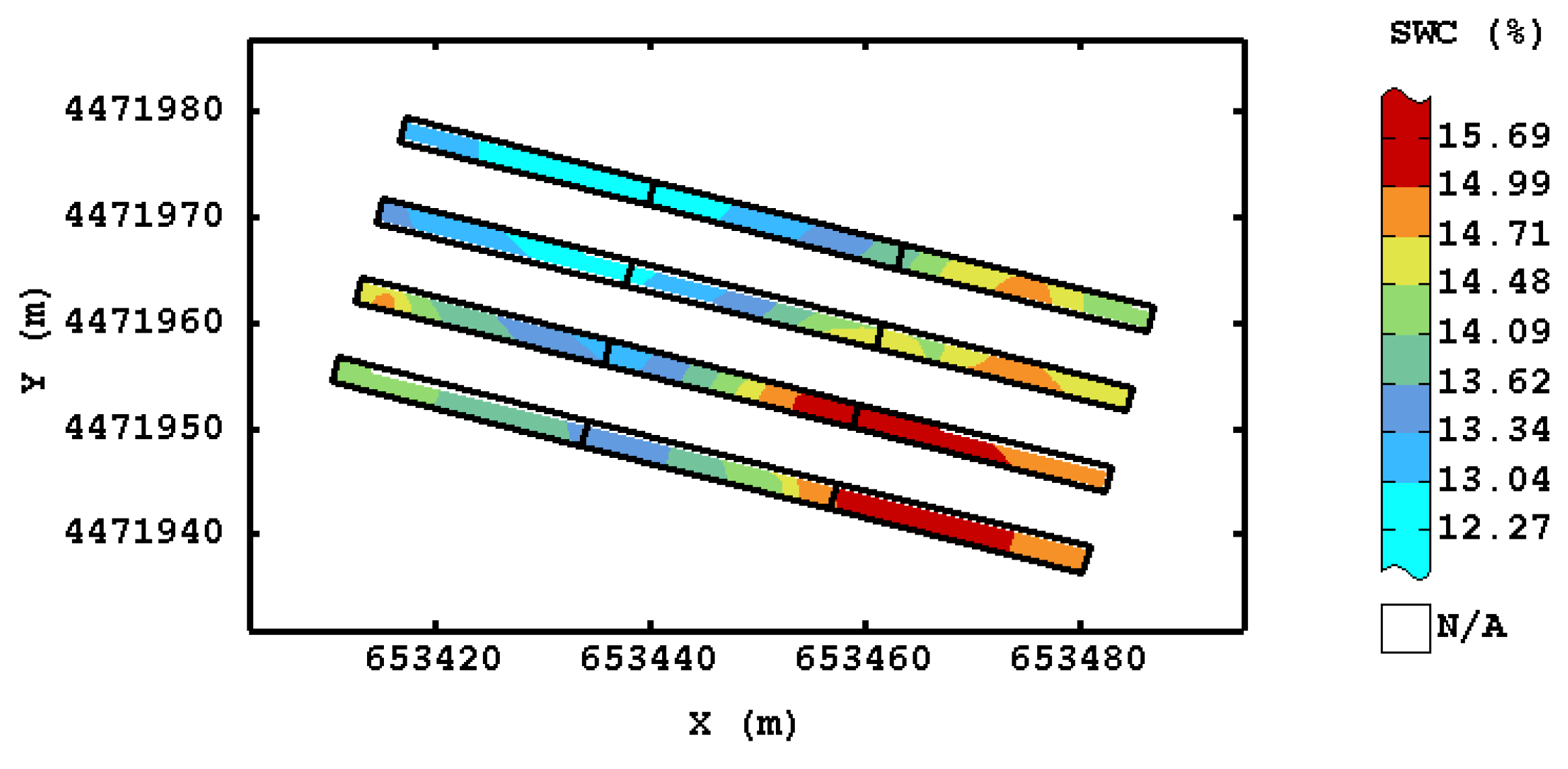
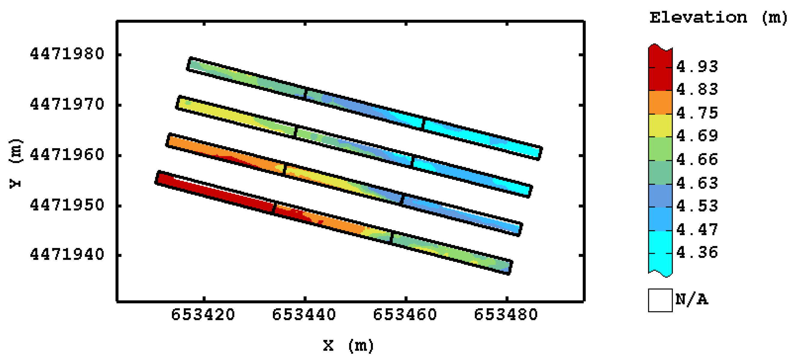
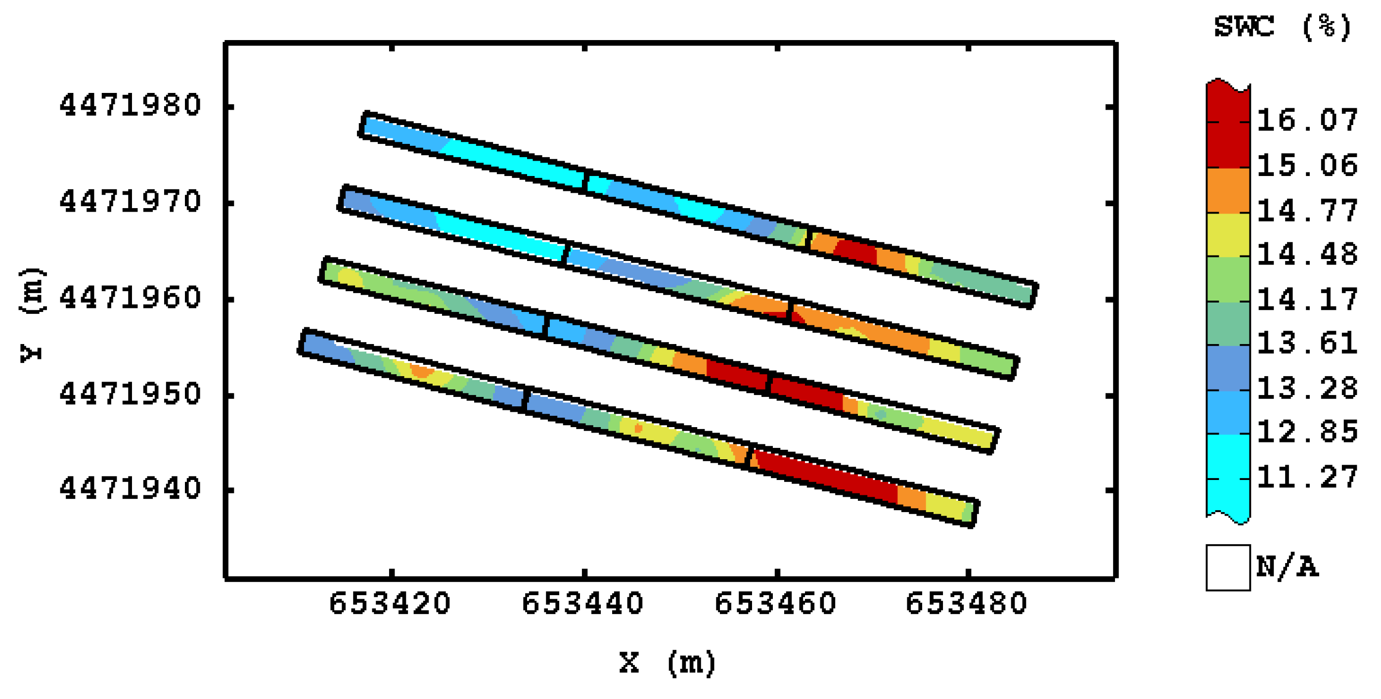
3.1. SWC and Eelevation Map
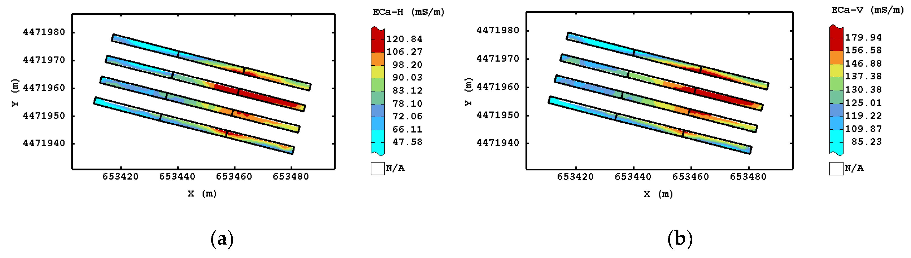
The SWC ranged between 11.26% and 17.37% with a range of spatial variation equal to 9.42. The data distribution indicated departure from normal distribution (the hypothesis of normality was refused based on χ2 test), therefore, the values were transformed into Gaussian scores and they were used for estimation. An isotropic model was fitted including a Nugget effect and a Spherical model (range = 59.5 m). The results of the cross-validation test were satisfactory because Mean Error was quite close to 0 (ME = 0.006) and the Mean Square Standardized Error was almost 1 (MSSE = 1.03).
The ordinary kriging (OK) SWC map showed higher values in the eastern portion of the field and in the south-western corner compared to the other parts of the field experiment (Figure 2). The coarse sampling scale likely determined the high degree of smoothness.
The elevation data looked positively skewed with sensible departure from normal distribution (the hypothesis of normality was refused based on χ2 test at the 5% level of probability (results not shown)) and they were previously transformed into Gaussian scores. An isotropic model was fitted including a Nugget effect and a Spherical model (range = 77 m). The lowest parts of the field corresponded to the highest values of SWC (Figure 3).

3.2. ECa Maps

The statistical distributions of ECa data in both orientations was skewed, so they were transformed into Gaussian scores. The two EMI variables were strongly correlated (r = 0.96), justifying the use of a multivariate approach. A linear model of coregionalization was fitted to the experimental variograms with a nugget effect and a cubic model (range of 100 m). The goodness of model fitting was considered satisfactory as both the mean error and the mean squared standardized error were close to zero and one, respectively.
Figure 4 shows the ECa-H and ECa-V maps, which were quite similar. Consequently, we found homogeneity between horizons (shallow and deep), although the correlation was partly due to deep ECa integrating the 1.5 m soil that includes the 0.75 m soil layer (represented by ECa-H) [37].
The ECa maps identified an area with the high electrical conductivities in the eastern portion of the field, while the western corner was characterized by lower values.
The overall accuracy, which ignores the spatial autocorrelation between observations, showed a fair agreement between ECa in both polarizations and SWC (54% and 47%, respectively). The cross-correlograms (Figure 5) showed that the maximum correlation between ECa in both polarizations and SWC was equal to ∼0.55, significant at a 0.05 probability level, but they were slightly asymmetric (not centered on lag zero). These results indicated that the locations of the sources of variation for EMI data were shifted with respect to the ones for SWC.

3.3. Ground Penetrating Radar Results

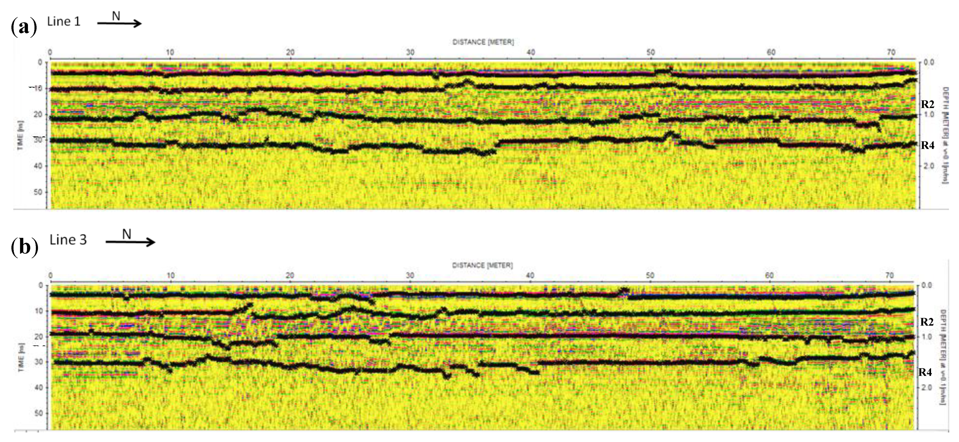
3.3.1. Radargrams Interpretation
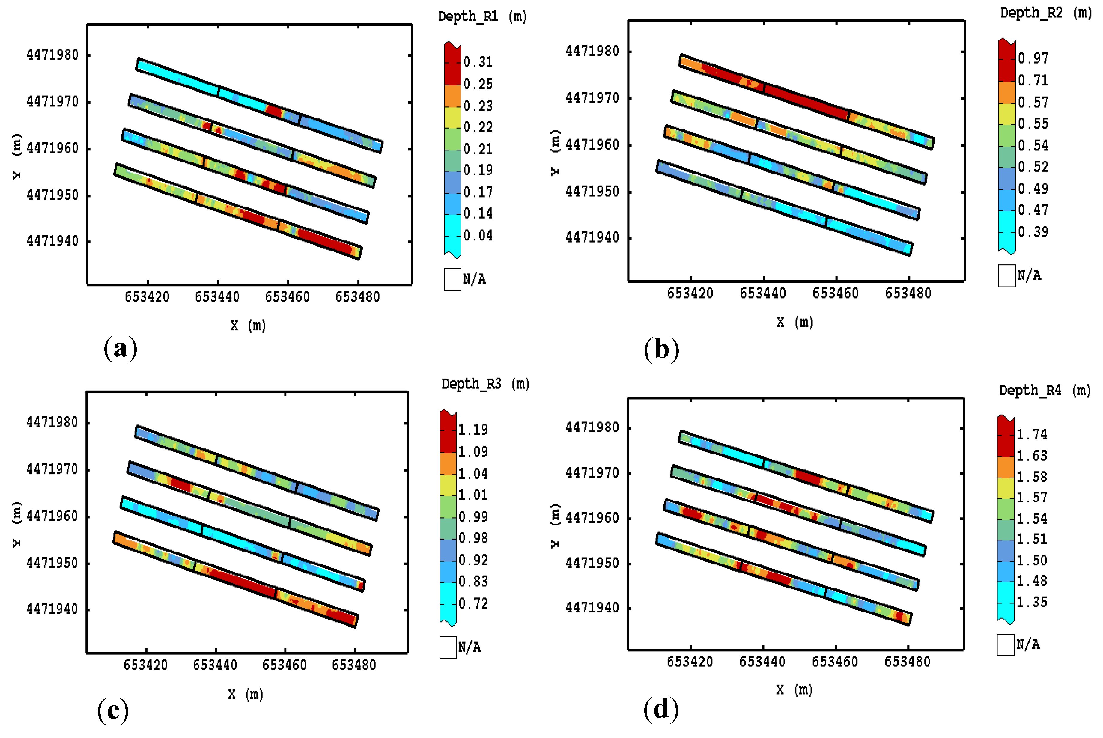
The radar sections (or radargrams), processed with a typical procedure sequence, exemplify the signal behavior recorded over the site. The estimated maximum depth investigated was about 2.5 m, considering that the average velocity of radio wave propagation was equal to 0.1 m ns−1. However, the profiles were not dominated by hyperbolas, indicating the absence of gravel content and stones, therefore, a more accurate velocity analysis should be considered.
On all radar sections, four reflection events, almost flat and continuous and sometimes interrupted, were easily identifiable. These events could be interpreted as due to the soil interfaces, considering their wide amplitude and denoting a strong electromagnetic contrast. In Figure 6, the following four main layers can be recognized: a first layer (R1) between about 0.1 and 7 ns (about 0–0.36 m), a second layer (R2) between about 7.2 and 20.5 ns (about 0.3–1 m), a third layer (R3) between about 13.4 and 26 ns (about 0.67–1.3 m) and a fourth one (R4) between about 25.4 and 36 ns (about 1.2–1.8 m). These reflections were consistent with the depth of layers identified in pre-existing pedological profile (Table 1). Under the last layer, there was high attenuation, which could be indicative of groundwater or an area holding moisture (wetting front), as shown in a previous study [24].
The radar signal displayed a uniform low-amplitude band between the two reflections, representing homogenous layers. Within the second and the third layers, the radar signal showed flat-lying reflections with some variation in amplitude, dip, and direction.
From the radar section of the same profile acquired with 1600 MHz frequency, only the first two reflections can be recognized, since the radar signal higher than 10 ns was attenuated (results not shown).
To evaluate the influence of soil discontinuities in spatial ECa and SWC variations, the apparent depths of reflections were extracted and interpolated using a multivariate approach [38]. A linear model of coregionalization, in which goodness of fitting was generally satisfactory, was fitted to the experimental variograms, including both a Nugget effect and a Spherical model, with a range of 23 m.
The cokriged maps (Figure 7) showed that the depth of the discontinuities varied along the profiles, therefore, the soil samples belonged to different soil layers. The first two maps (Figure 7a,b) represented the depths involved directly in the sampling and they show a difference between the first two soil strips and the last two ones. The third reflection shows the depth of the layer as a horizon with a lower permeability to water (Figure 7c). This layer was not directly involved in the sampling, but its presence and depth influenced the geophysical measurements that investigated a large volume of soil compared to soil samples. The fourth map represented the depth of the fourth reflection (R4, between 1.35 and 1.74 m), which corresponded to the effective depth range of ECa obtained in vertical polarizations (Figure 7d).
Figure 8 shows the correlation between SWC and the depth of R2, because it represents the beginning of the layer interpreted as horizon with lower permeability and which, therefore, could influence the vertical flux of water. The correlation was negative with the maximum correlation equal to –0.5 and the cross-correlograms showed enough symmetry around the lag zero.

3.3.2. GPR Maps

The GPR sections showed both great coherency and lateral continuity. Only some parts of the sections had a relatively unclear GPR or attenuated signal, which corresponded to low values of electrical conductivity. Therefore, the amplitude maps were created, which were one of the best methods to display GPR data as horizontal maps.
The time slices for 600 MHz antenna were built within consecutive time windows of 2 to 10 ns, since the antenna showed a sensible attenuation of signal at about 10 ns (equal to about 0.50 m depth). All successive procedures of variography and interpretation will be applied up to this depth. The amplitude maps for 1600 MHz antenna were built within consecutive time windows of 1 to 5.5 ns (equal to about 0.27 m). The data for the 1600 MHz antenna showed lower values compared to the other antenna.
All of the GPR data at any time interval and for each antenna were correlated among them, in order to justify the multivariate approach. The data were previously transformed into standard Gaussian variables and an LMC was fitted to all experimental direct variogram and cross-variograms (separately for each antenna). The LMCs consisted of the following basic structures: (1) for 600 MHz: Nugget effect and two Spherical models at 10 and 33 m Range, respectively; (2) for 1600 MHz: Nugget effect and two Spherical models at 9 and 33 m Range, respectively. Mean error was quite close to 0 and the mean square standardized error was almost 1 for all data sets.
The map of the estimated amplitude for 600 MHz antenna at 0.30 m depth (Figure 9a) showed the same division of the field with a tendency towards low amplitude signals in the eastern part of the field, except the third strip, probably due to the variations in soil depth. In the third strip, the area with higher values of amplitudes corresponded to higher values of ECa in both polarizations.
The map of the estimated amplitude for 1600 MHz antenna at 0.27-m depth (Figure 9b) showed low amplitude signals in the first two strips (southern part of the field) and a relative high amplitude in the last two strips, reproducing approximately the structures of R1 and R2 with negative correlation.

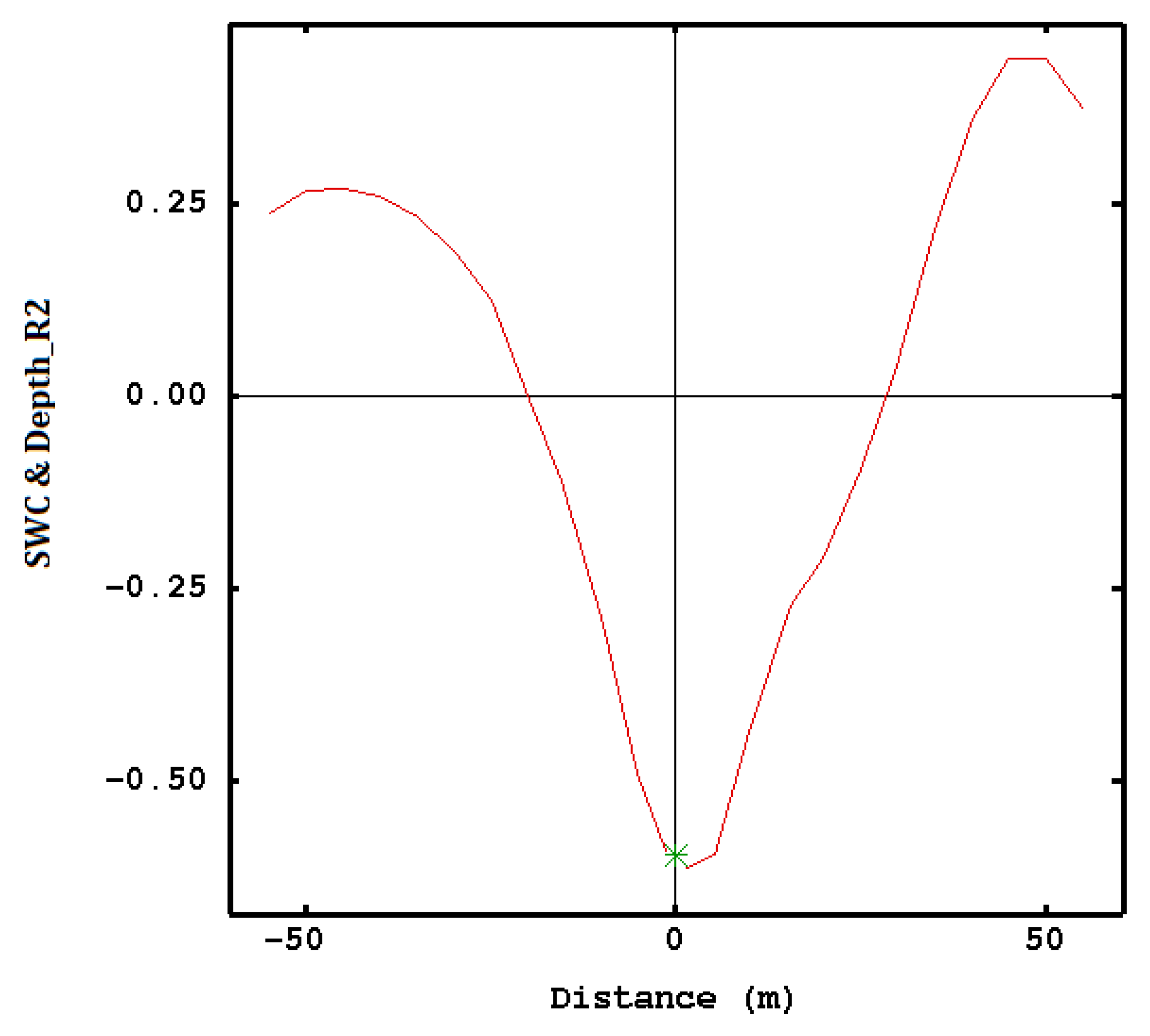
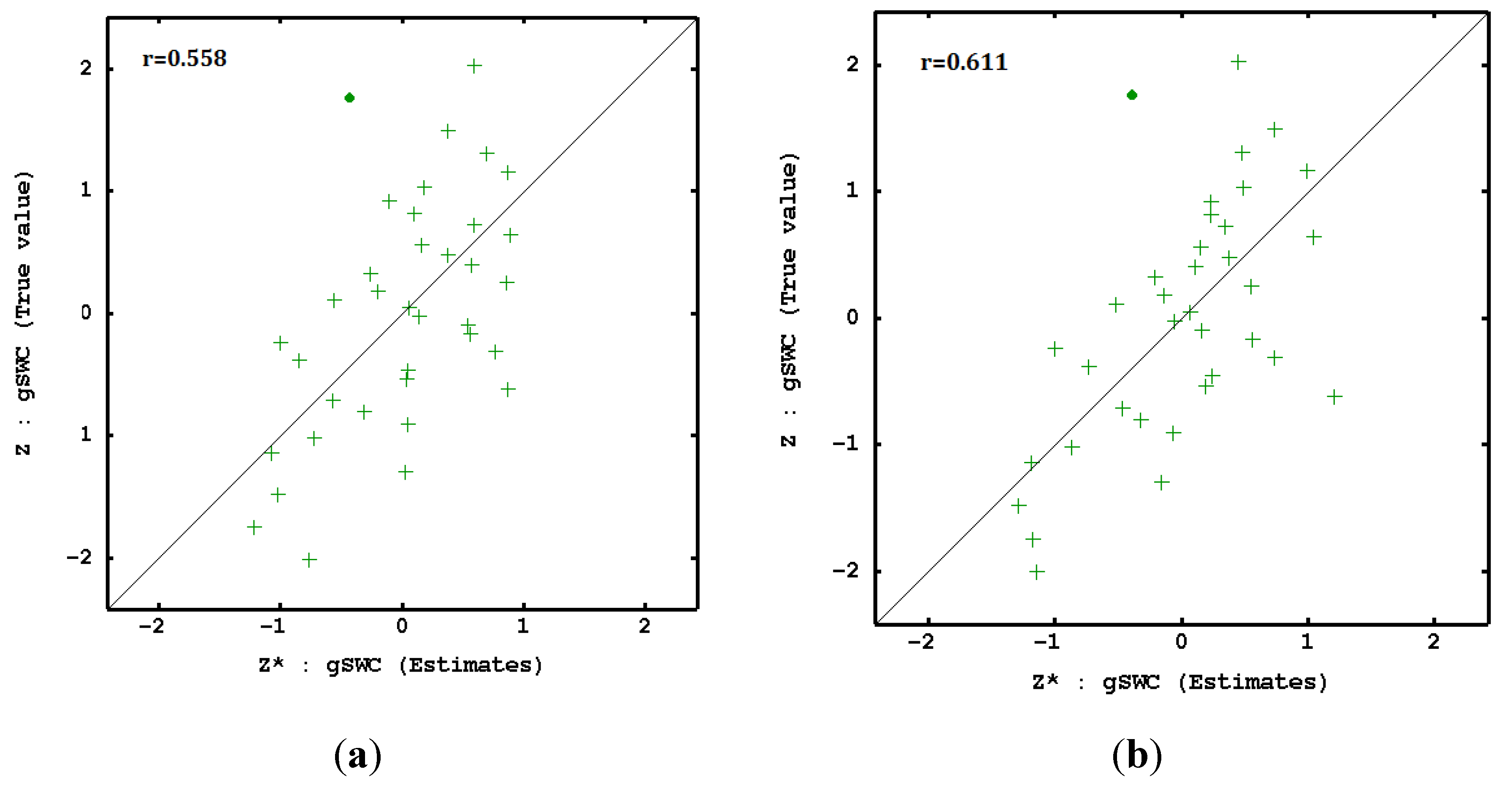
3.4. Spatial Prediction of SWC with Geophysical Parameters

The stepwise regression selected ECa in both polarizations, 1600 antenna slices at 0.27 m depth and the depth of R3 as significant regressors of SWC estimation with R2 = 0.64 and with the probability level <0.15. The correlation analysis showed that the strongest correlation occurred between soil water content and ECa-H, therefore, the latter was chosen as the collocated variable in the successive interpolation procedure. To avoid large spikes in the experimental variograms, all variables were transformed by Gaussian anamorphosis. The experimental variograms did not show clear anisotropy, therefore, before applying cokriging an intrinsic stationarity was assumed and an isotropic LMC was fitted. The LMC included a Nugget effect, a Spherical model (Range = 10 m), and a Cubic model (range = 100 m).
Figure 10 shows the MCCOK map. Comparing the maps of SWC obtained with MCCOK with the one with OK (Figure 2), it seems that the two types of maps reproduce the same main structures of spatial dependence. The increased variability observed in the MCCOK map can be explained considering the fine-scale variation determined by geophysical data.
For a direct comparison, the OK and MCCOK estimates through the cross-validation were plotted with respect to the measured SWC values. MCCOK provided a slightly better fit as confirmed by the higher correlation coefficient (r = 0.61) in comparison with OK (r = 0.55) and the data were more gathered around the 1:1 line (Figure 11).

4. Discussion

4.1. SWC and ECa Maps

The small SWC range of spatial variation could be attributed to the limited extension of the tested area as well as to the small heterogeneity of soil texture [39]. The highest values of SWC corresponded to the lowest parts of the field. This result was obtained despite there being no topographic variations in the study area, with no remarkable differences in height between the two areas (of about 0.6 m of the maximum difference). It was clear that the soil hydraulic arrangement did not eliminate completely the risk of water stagnation.
However, since the spatial patterns of SWC could have been influenced by the variations in soil depth and soil/bedrock interface [40], the combination of different sensors and integrating their data could discriminate whether or not agronomical factors (hydraulic arrangement, organic amendment application, etc.) can modify SWC distribution [41], and could also provide its more accurate estimation [42]. The ECa maps identified an area with the highest electrical conductivities in the eastern part of the field, while the western corner was characterized by lower values. Considering that the maps were produced when the soil was bare and after a spring–summer organic zucchini cultivation, the spatial patterns might reflect differences in topography, soil texture, and water content [11,12].
From visual comparison, the maps of the ECa were like those of the SWC (Figure 2), also following the same spatial pattern of digital elevation model (Figure 3). A higher soil electrical conductivity can be observed in lower areas (negative correlation between ECa and elevation, r = −0.6), where the soil water content tended to be naturally high, as shown by Serrano et al. [43]. In general, surface topography plays a substantial role in influencing spatial variation of ECa. The level and location of both runoff and infiltration are determined by field elevation, which locally can influence the variation in water content. Where the elevation is slightly high, the SWC is lower than in areas where depression occurs [44].
However, the overall accuracy and the cross correlogram between the ECa data in both polarizations and SWC showed a weak correlation, confirming the homogeneity between shallow and deep horizons and an indirect not unique relationship between these variables, but it likely depended on many other factors [45,46]. This result suggested that the variability of the moisture content did not significantly influence the variability of the ECa and, probably, the correlation could be the highest with other soil properties. Therefore, although previous studies refer to the influence of soil moisture on electrical conductivity [47,48,49], the findings of this research indicated limitations for the use of EMI sensors as an indicator of SWC and that one sensor alone cannot achieve a good estimation of soil spatial variation [41,42]. Since both the surface topography and the soil discontinuities play an important role in influencing spatial ECa variation [50], the radargram analysis and interpretation might help to identify soil discontinuities and their depths. Therefore, we identified depths of soil discontinuities by interpretation of GPR radargrams, as well as amplitude of GPR signal data at two different frequencies.

4.2. Ground Penetrating Radar

Variations in the electrical properties of soils mainly depend on moisture content [51] and these contrasts produce strong reflections on the most radar records [16]. Our results show that the lines of contrast that we found between the second and the third layers were consistent along the soil profiles at about the same depth, and this layer could be interpreted as a horizon with lower permeability to water. These reflections were probably not due to change in subsurface material such as soil texture, but were due to micro-porosity, hydraulic conductivity, and subsurface structure (distribution of materials and layering) [52]. From the visual inspection of the radargrams, the different antennas showed results varying in terms of resolution, but one antenna was not selected because each one provided useful information for this study.
The cokriged map showed the same division of the field observed in the EMI and elevation maps with negative correlations, suggesting that EMI measurement can be affected by the soil profile, also confirming that ECa values are integrated values on all profiles. The correlation between SWC and the different depth was negative, and this result was likely due to the water content stored in areas with shallower layer. The low permeability was also larger than the total water content stored in the area with this deeper layer, as a consequence of the absence of water leaching. Therefore, the variations in soil discontinuity could significantly affect the spatial distribution of SWC [53].
From visual inspection, the amplitude maps for 600 MHz antenna showed the same spatial pattern of EMI and SWC maps, showing that the soils with higher water results and conductivity values have higher radar signal attenuation (or lower radar reflectance) [54]. This seemed to be a surprising result because it is expected that an increase in soil water will attenuate the radar signal. One of the possible explanations of this result could be a higher degree of soil compaction, which caused the reflection of the radar signal, but also held back the water, indicating an increase in electrical conductivity [55]. However, further investigations are needed to verify the pedological profile. The maps of the estimated amplitude for the 1600 MHz antenna did not show similar spatial structures in comparison with those of the 600 MHz antenna, due to its finer spatial resolution. These results might be related to a short-range variability in micro-structures, which the GPR system with the 600 MHz antenna did not detect. Therefore, to capture the scale-dependent variability of the soil there was the need to use antennas of different frequency [27].
The cross-correlations between SWC and GPR data were very low and positive and the shape was a little skewed (results not shown). This seemed a surprising result because it is expected that an increase in soil water will attenuate the radar signal. In any case, this behavior could be due to a quite complex and multiphase system, since soil moisture is affected by so many interacting factors that only a multivariate nonlinear model can produce a reliable prediction [42,56]. Despite the success of this technique in its initial development and application for geological inspection, it has several drawbacks if the objective is the prediction of SWC uniquely from the GPR data. The estimates are too uncertain because of the complexity of the surveyed subsoil. Therefore, only fusing data from different sensors and using geophysical data as auxiliary information could produce more reliable predictions of SWC [40].

4.3. Spatial Prediction of SWC with Geophysical Parameters

The results of the stepwise regression indicated as significant regressors of SWC estimation the ECa in both polarizations, 1600 antenna slices at 0.27 m depth and the depth of R3. The strongest correlation occurred between soil water content and ECa-H, therefore, the latter was chosen as the co-located variable in the successive interpolation procedure. These results showed that the EMI sensor was a useful indicator for shallow SWC, explaining most of its variation, whereas only a little information derived from the GPR data partially affected its estimation. However, these results showed the statistical significance of the geophysical variables in soil water content prediction as shown in previous studies [20,42].
The effectiveness of using sensor systems in combination instead of a single sensor is relative, since proximal sensing data are often massive, with different spatial and temporal precision, and different measurement supports and subject to measurement error biases. Literature on this topic is still weak [57], therefore, using techniques that combine data from multiple sources, as we did in this research, achieving inferences on soil moisture, can be considered an innovative approach. Moreover, unlike standard statistical approach, such as regression methods that have been extensively applied to analyze soil variables and their relations with other covariates, geostatistical techniques are based on assessing and modelling of auto-correlation function of the spatial variable [33].

5. Conclusions

Electromagnetic induction instruments are known to be effective tools in reflecting soil moisture changes through the variations in ECa. Even if one year is not enough to draw general conclusions, our study confirmed this result. However, the main limitation of this sensor is that its outcomes are integrated values over all soil layers. The results also highlighted that the GPR radargrams and amplitude maps have proved that it is possible to extract useful information on soil discontinuity in a noninvasive way. Moreover, the combined use of these sensors helped the interpretation of the results, and their integration may potentially help overcoming the intrinsic limitation of the two methods.
On the other hand, in a complex system such as an organic cultivated soil, the relationship between geophysical sensors and the SWC may not be linear and therefore the geophysical sensors have several limitations for a direct prediction of SWC. However, the geophysical data applied in this research will be used as auxiliary variables to estimate soil water content through a geostatistical technique, to allow its accurate estimation and to explore the potential of the method to include the geophysical information for SWC prediction. From an agronomic point of view, the knowledge of soil attributes which influence SWC could also be important to ensure the stability of crop production, even in the presence of temporary flooding caused by frequent extreme rainfall events.
Future work should also focus on measurements repeated in different water conditions for both sensors, because they can provide information about highly dynamic soil attributes (such as soil structure).

Author Contributions

Conceptualization, D.B.D., M.F., and D.M.; methodology, D.B.D.; writing—original draft preparation, D.B.D., M.F., and D.M.; writing—review and editing, D.B.D. and D.M.; funding acquisition, M.F.

Funding

This research was funded by the Organic Farming Office of the Italian Ministry of Agriculture.

Acknowledgments

This paper is a result of the AGROCAMBIO (Sistemi e tecniche AGROnomiche di adattamento ai CAMbiamenti climatici in sistemi agricoli BIOlogici) and RETIBIO (Attività di supporto nel settore dell’agricoltura biologica per il mantenimento dei dispositivi sperimentali di lungo termine e il rafforzamento delle reti di relazioni esistenti a livello nazionale e internazionale) research projects.

Conflicts of Interest

The authors declare no conflict of interest. The funders had no role in the design of the study; in the collection, analyses, or interpretation of data; in the writing of the manuscript, or in the decision to publish the results.

References

  1. Montemurro, F.; Persiani, A.; Diacono, M. Environmental sustainability assessment of horticultural systems: A multi-criteria evaluation approach applied in a case study in Mediterranean conditions. Agronomy 2018, 8, 98. [Google Scholar] [CrossRef]
  2. Diacono, M.; Persiani, A.; Fiore, A.; Montemurro, F.; Canali, S. Agro-ecology for adaptation of horticultural systems to climate change: Agronomic and energetic performance evaluation. Agronomy 2017, 7, 35. [Google Scholar] [CrossRef]
  3. Vereecken, H.; Huisman, J.A.; Bogena, H.; Vanderborght, J.; Vrugt, J.A.; Hopmans, J.W. On the value of soil moisture measurements in vadose zone hydrology: A review. Water Resour. Res. 2008, 44, W00D06. [Google Scholar] [CrossRef]
  4. De Benedetto, D.; Montemurro, F.; Diacono, M. Impacts of agro-ecological practices on soil losses and cash crop yield. Agriculture 2017, 7, 103. [Google Scholar] [CrossRef]
  5. Rubin, Y. Soil Water Monitoring Using Geophysical Techniques: Development and Applications in Agriculture and Water Resources Management; Technical Completion Reports; University of California: Berkeley, CA, USA, 2003. [Google Scholar]
  6. Yoder, R.E.; Freeland, R.S.; Ammons, J.T.; Leonard, L.L. Mapping agricultural fields with GPR and EMI to identify offsite movement of agrochemicals. J. Appl. Geophys. 2001, 47, 251–259. [Google Scholar] [CrossRef]
  7. Algeo, J.; Slater, L.; Binley, A.; van Dam, R.L.; Watts, C. A comparison of ground-penetrating radar early-time signal approaches for mapping changes in shallow soil water content. Vadose Zone J. 2018, 17, 1. [Google Scholar] [CrossRef]
  8. Viscarra Rossel, R.A.; Adamchuk, V.I.; Sudduth, K.A.; McKenzie, N.J.; Lobsey, C. Proximal soil sensing: An effective approach for soil measurements in space and time. Adv. Agron. 2011, 113, 243–291. [Google Scholar] [CrossRef]
  9. Corwin, D.L.; Lesch, S.M. Application of soil electrical conductivity to precision agriculture: Theory, principles, and guidelines. Agron. J. 2003, 95, 455–471. [Google Scholar] [CrossRef]
  10. Reedy, R.C.; Scanlon, B.R. Soil water content monitoring using electromagnetic induction. J. Geotech. Geoenviron. Eng. 2003, 129, 1–12. [Google Scholar] [CrossRef]
  11. Brevik, E.C.; Fenton, T.E.; Lazari, A. Soil electrical conductivity as a function of soil water content and implications for soil mapping. Precis. Agric. 2006, 7, 393–404. [Google Scholar] [CrossRef]
  12. De Benedetto, D.; Castrignanò, A.; Diacono, M.; Rinaldi, M.; Ruggieri, S.; Tamborrino, R. Field partition by proximal and remote sensing data fusion. Biosyst. Eng. 2013, 114, 372–383. [Google Scholar] [CrossRef]
  13. Lunt, I.A.; Hubbard, S.S.; Rubin, U. Soil moisture estimation using ground penetrating radar reflection data. J. Hydrol. 2005, 307, 254–269. [Google Scholar] [CrossRef]
  14. Galagedara, L.W.; Parkin, G.W.; Redman, J.D.; von Bertoldi, P.; Endres, A.L. Field studies of the GPR ground wave method for estimating soil water content during irrigation and drainage. J. Hydrol. 2005, 301, 182–197. [Google Scholar] [CrossRef]
  15. Liu, X.; Chen, J.; Cui, X.; Liu, Q.; Cao, X.; Chen, X. Measurement of soil water content using ground-penetrating radar: A review of current methods. Int. J. Digit. Earth 2019, 12, 95–118. [Google Scholar] [CrossRef]
  16. Daniels, D.J. Ground Penetrating Radar, 2nd ed.; The Institution of Engineering and Technology: London, UK, 2004. [Google Scholar]
  17. Grote, K.; Anger, C.; Kelly, B.; Hubbard, S.; Rubin, Y. Characterization of soil water content variability and soil texture using GPR groundwave techniques. J. Environ. Eng. Geophys. 2010, 15, 93–110. [Google Scholar] [CrossRef]
  18. Hubbard, S.; Grote, K.; Rubin, Y. Mapping the volumetric soil water content of a California vineyard using high-frequency GPR ground wave data. Lead. Edge 2002, 25, 552–559. [Google Scholar] [CrossRef]
  19. Knight, R.; Tercier, P.; Jol, H. The role of ground-penetrating radar and geostatistics in reservoir description. Lead. Edge 1997, 16, 1576–1582. [Google Scholar] [CrossRef]
  20. De Benedetto, D.; Castrignanò, A.; Sollitto, D.; Modugno, F.; Buttafuoco, G.; Lo Papa, G. Integrating geophysical and geostatistical techniques to map the spatial variation of clay. Geoderma 2012, 171–172, 53–63. [Google Scholar] [CrossRef]
  21. Diacono, M.; Fiore, A.; Farina, R.; Canali, S.; Di Bene, C.; Testani, E.; Montemurro, F. Combined agro-ecological strategies for adaptation of organic horticultural systems to climate change in Mediterranean environment. Ital. J. Agron. 2016, 11, 730–785. [Google Scholar] [CrossRef]
  22. Soil Survey Staff USA. Soil Taxonomy: A Basic System of Soil Classification for Making and Interpreting Soil Surveys, 2nd ed.; Agriculture Handbook No. 436; Government Printing Office: Washington, DC, USA, 1999.
  23. UNESCO-FAO. Etude Écologique de la Zone Méditerranéenne. Carte Bioclimatique de la Zone Méditerranéenne. [Ecological Study of the Mediterranean Area: Bioclimatic Map of the Mediterranean Sea]. Paris-Rome. 1963. Available online: http://unesdoc.unesco.org/ images/0013/001372/137255fo.pdf (accessed on 3 January 2019).
  24. Ventrella, D.; Mohanty, B.P.; Simunek, J.; Losavio, N.; van Genuchten, M.T. Water and chloride transport in a fine-textured soil: Field experiments and modelling. Soil Sci. 2000, 165, 624–631. [Google Scholar] [CrossRef]
  25. Topp, G.C.; Davis, J.L.; Annan, A.P. Electromagnetic determination of soil water content: Measurements in coaxial transmission lines. Water Resour. Res. 1980, 16, 574–582. [Google Scholar] [CrossRef] [Green Version]
  26. De Benedetto, D.; Castrignanò, A.; Sollitto, D.; Modugno, F. Spatial relationship between clay content and geophysical data. Clay Miner. 2010, 45, 197–207. [Google Scholar] [CrossRef]
  27. De Benedetto, D.; Quarto, R.; Castrignanò, A.; Palumbo, D.A. Impact of data processing and antenna frequency on spatial structure modelling of GPR data. Sensors 2015, 15, 16430–16447. [Google Scholar] [CrossRef] [PubMed]
  28. Sandmeier Scientific Software. Reflexw, v.6.1.1, program for processing and interpretation of reflection and transmission data. User’s Manual Online Version, Karlruhe, Germany, 2012. [Google Scholar]
  29. Journel, A.; Huijbregts, C. Mining Geostatistics; Academic Press: London, UK, 1978. [Google Scholar]
  30. Cressie, N.A.C. Statistics for Spatial Data; Wiley & Sons: New York, NY, USA, 1991. [Google Scholar]
  31. Goovaerts, P. Geostatistics for Natural Resources Evaluation; Applied Geostatistics Series; Oxford University Press: Oxford, UK, 1997. [Google Scholar]
  32. SAS Institute Inc. 2013 SAS/STAT Software Release 9.3; SAS Institute Inc.: Cary, NC, USA, 2013. [Google Scholar]
  33. Rivoirard, J. Which models for collocated cokriging? J. Math. Geol. 2001, 33, 117–131. [Google Scholar] [CrossRef]
  34. Geovariances. Isatis Technical Ref.; ver. 2013.1; Geovariances & Ecole Des Mines De Paris: Avon CEDEX, France, 2015. [Google Scholar]
  35. Campbell, J. Introduction to Remote Sensing, 3rd ed.; The Guilford Press: New York, NY, USA, 2002. [Google Scholar]
  36. Kravchenko, A.N.; Omonode, R.; Bollero, G.A.; Bullock, D.G. Quantitative mapping of soil drainage classes using topographical data and soil electrical conductivity. Soil Sci. Soc. Am. J. 2003, 66, 235–243. [Google Scholar] [CrossRef]
  37. De Caires, S.A.; Wuddivira, M.N.; Bekele, I. Assessing the temporal stability of spatial patterns of soil apparent electrical conductivity using geophysical methods. Int. Agrophysics 2014, 28, 423–433. [Google Scholar] [CrossRef]
  38. Wackernagel, H. Multivariate Geostatistics: An Introduction with Applications; Springer: Berlin, Germany, 2003. [Google Scholar]
  39. Warrick, A.W.; Nielsen, D.R. Spatial Variability of Soil Physical Properties in the Field; Academic Press: New York, NY, USA, 1980; pp. 319–344. [Google Scholar]
  40. De Benedetto, D.; Castrignanò, A.; Quarto, R. A geostatistical approach to estimate soil moisture as a function of geophysical data and soil attributes. Procedia Environ. Sci. 2013, 19, 436–445. [Google Scholar] [CrossRef]
  41. De Benedetto, D.; Montemurro, F.; Diacono, M. Repeated geophysical measurements in dry and wet soil conditions to describe soil water content variability. Sci. Agric. 2019, in press. [Google Scholar]
  42. Barca, E.; De Benedetto, D.; Stellacci, A.M. Contribution of EMI and GPR proximal sensing data in soil water content assessment by using linear mixed effects models and geostatistical approaches. Geoderma 2019, 343, 280–293. [Google Scholar] [CrossRef]
  43. Serrano, J.M.; Peça, J.O.; Marques da Silva, J.R.; Shaidian, S. Mapping soil and pasture variability with an electromagnetic induction sensor. Comput. Electron. Agric. 2010, 73, 7–16. [Google Scholar] [CrossRef]
  44. Appels, W.M.; Bogaart, P.W.; van der Zee, S. Influence of spatial variations of microtopography and infiltration on surface runoff and field scale hydrological connectivity. Adv. Water Resour. 2011, 34, 303–313. [Google Scholar] [CrossRef]
  45. Zhu, Q.; Lin, H.; Doolittle, J. Repeated electromagnetic induction surveys for determining subsurface hydrologic dynamics in an agricultural landscape. Soil Sci. Soc. Am. J. 2010, 74, 1750–1762. [Google Scholar] [CrossRef]
  46. Martini, E.; Werban, U.; Zacharias, S.; Pohle, M.; Dietrich, P.; Wollschläger, U. Repeated electromagnetic induction measurements for mapping soil moisture at the field scale: Validation with data from a wireless soil moisture monitoring network. Hydrol. Earth Syst. Sci. 2017, 21, 495–513. [Google Scholar] [CrossRef]
  47. Johnson, C.; Eskridge, K.; Corwin, D. Apparent soil electrical conductivity: Applications for designing and evaluating field-scale experiments. Comput. Electron. Agric. 2005, 46, 181–202. [Google Scholar] [CrossRef]
  48. King, J.; Dampney, P.; Lark, R.; Wheeler, H.; Bradley, R.; Mayr, T. Mapping potential crop management zones within fields: Use of yield-map series and pat-terns of soil physical properties identified by electromagnetic induction sensing. Precis. Agric. 2005, 6, 167–181. [Google Scholar] [CrossRef]
  49. Bronson, K.; Booker, J.; Officer, S.; Lascano, R.; Maas, S.; Searcy, S.; Booker, J. Apparent electrical conductivity, soil properties and spatial covariance in the U.S. southern high plains. Precis. Agric. 2005, 6, 297–311. [Google Scholar] [CrossRef]
  50. Corwin, D.L.; Plant, R.E. Applications of apparent soil electrical conductivity in precision agriculture. Comput. Electron. Agric. 2005, 46, 1–10. [Google Scholar] [CrossRef]
  51. Annan, A.P.; Cosway, S.W.; Redman, J.D. Water table detection with ground-penetrating radar. In Proceedings of the SEG 61st Annual Meeting, Houston, TX, USA, January 1991. [Google Scholar]
  52. Comite, D.; Galli, A.; Lauro, S.E.; Mattei, E.; Pettinelli, E. Analysis of GPR early-time signal features for the evaluation of soil permittivity through numerical and experimental surveys. IEEE J. Sel. Top. Appl. Earth Obs. Remote Sens. 2016, 9, 178–187. [Google Scholar] [CrossRef]
  53. Algeo, J.; Van Dam, R.L.; Slater, L. Early-time GPR: A method to monitor spatial variations in soil water content during irrigation in clay soils. Vadose Zone J. 2016, 15, 1–9. [Google Scholar] [CrossRef]
  54. Hendrickx, J.M.H.; Hong, S.-H.; Miller, T.; Borchers, B.; Reberghen, J.B. Soil effects on GPR detection of buried non-metallic mines. Ground penetrating radar in sediments. Geol. Soc. Lond. Special Publ. 2003, 211, 191–198. [Google Scholar] [CrossRef]
  55. Wang, P.; Hu, Z.; Zhao, Y.; Li, X. Experimental study of soil compaction effects on GPR signals. J. Appl. Geophys. 2016, 126, 128–137. [Google Scholar] [CrossRef]
  56. Cafarelli, B.; Castrignanò, A.; De Benedetto, D.; Palumbo, A.D.; Buttafuoco, G. A linear mixed effect (LME) model for soil water content estimation based on geophysical sensing: A comparison of an LME model and kriging with external drift. Environ. Earth Sci. 2015, 73, 1951–1960. [Google Scholar] [CrossRef]
  57. Taylor, J.A.; Short, M.; McBratney, A.B.; Wilson, J. Comparing the ability of multiple soil sensors to predict soil properties in a Scottish potato production system. In Proximal Soil Sensing: Progress in Soil Science; Viscarra Rossel, R.A., McBratney, A.B., Minasny, B., Eds.; Springer Science +Business Media, B.V.: Dordrecht, The Netherlands, 2010; Volume 1, pp. 387–396, Part 5. [Google Scholar]
Figure 1. The field experiment with the soil water content (SWC) sampling locations (green dots) the electromagnetic induction (EMI) (blue dashed lines) and Ground Penetrating Radar (GPR) acquisitions along transects (red lines).
Agronomy 09 00638 g001
Figure 2. Spatial estimates of gravimetric SWC obtained with ordinary kriging (OK). Color scale uses iso-frequency classes.
Agronomy 09 00638 g002
Figure 3. Spatial estimates of a Differential Global Positioning System (DGPS) height. Color scale uses iso-frequency classes.
Agronomy 09 00638 g003
Figure 4. Spatial estimate of apparent electrical conductivity (ECa) in (a) horizontal and (b) vertical polarization. Color scale uses iso-frequency classes.
Agronomy 09 00638 g004
Figure 5. Cross correlogram between SWC and ECa in (a) horizontal polarization and ECa in (b) vertical polarization. Correlation coefficients at lag 0 are significant at a 0.05 probability level.
Agronomy 09 00638 g005
Figure 6. GPR profiles acquired with the 600 MHz antenna along (a) the first strip and (b) the third strip.
Agronomy 09 00638 g006
Figure 7. The cokriged maps for depths of soil discontinuities: (a,b) represent the depths involved directly in the sampling; (c) is the layer not directly involved in the sampling; (d) represents the depth of the fourth reflection (R4, between 1.35 and 1.74 m), which corresponded to the effective depth range of ECa obtained in vertical polarizations. Color scale uses iso-frequency classes.
Agronomy 09 00638 g007
Figure 8. Cross correlogram between SWC and the depth of second reflection (Depth_R2). Correlation coefficients at lag 0 are significant at a 0.05 probability level.
Agronomy 09 00638 g008
Figure 9. Estimated amplitude maps for the 600 MHz antenna at (a) 0.30 m and amplitude maps for the 1600 MHz antenna at (b) 0.27m.
Agronomy 09 00638 g009
Figure 10. Spatial estimate of SWC obtained with multi-collocated cokriging.
Agronomy 09 00638 g010
Figure 11. Scatter diagram of the measured SWC data versus the estimated values by (a) OK and (b) multi-collocated cokriging (MCCOK) through cross-validation.
Agronomy 09 00638 g011
Table 1. Soil properties of the representative profile in the experimental farm.
HorizonDepth (m)Particle Size Distribution
Clay (%)Silt (%)Sand (%)
Ap0–(0.30–0.50)58.835.85.50
Abss(0.30–0.50)–0.7060.035.84.23
Abssk0.70–160.236.43.51
Bw1–1.7067.730.81.53
Btg1.70–2.1077.222.00.84

