Article

In-Season Diagnosis of Winter Wheat Nitrogen Status in Smallholder Farmer Fields Across a Village Using Unmanned Aerial Vehicle-Based Remote Sensing

1
School of Surveying and Land Information Engineering, Henan Polytechnic University, Jiaozuo 454000, China
2
International Center for Agro-Informatics and Sustainable Development (ICASD), College of Resources and Environmental Sciences, China Agricultural University, Beijing 100193, China
3
Precision Agriculture Center, Department of Soil, Water and Climate, University of Minnesota, St. Paul, MN 55108, USA
4
Center for Precision Agriculture, Norwegian Institute of Bioeconomy Research (NIBIO), Nylinna 226, 2849 Kapp, Norway
*
Author to whom correspondence should be addressed.
Agronomy 2019, 9(10), 619; https://doi.org/10.3390/agronomy9100619
Submission received: 4 September 2019 / Revised: 30 September 2019 / Accepted: 4 October 2019 / Published: 9 October 2019
(This article belongs to the Special Issue Precision Agriculture)

Abstract

:
Improving nitrogen (N) management of small-scale farming systems in developing countries is crucially important for food security and sustainable development of world agriculture, but it is also very challenging. The N Nutrition Index (NNI) is a reliable indicator for crop N status, and there is an urgent need to develop an effective method to non-destructively estimate crop NNI in different smallholder farmer fields to guide in-season N management. The eBee fixed-wing unmanned aerial vehicle (UAV)-based remote sensing system, a ready-to-deploy aircraft with a Parrot Sequoia+ multispectral camera onboard, has been used for applications in precision agriculture. The objectives of this study were to (i) determine the potential of using fixed-wing UAV-based multispectral remote sensing for non-destructive estimation of winter wheat NNI in different smallholder farmer fields across the study village in the North China Plain (NCP) and (ii) develop a practical strategy for village-scale winter wheat N status diagnosis in small scale farming systems. Four plot experiments were conducted within farmer fields in 2016 and 2017 in a village of Laoling County, Shandong Province in the NCP for evaluation of a published critical N dilution curve and for serving as reference plots. UAV remote sensing images were collected from all the fields across the village in 2017 and 2018. About 150 plant samples were collected from farmer fields and plot experiments each year for ground truthing. Two indirect and two direct approaches were evaluated for estimating NNI using vegetation indices (VIs). To facilitate practical applications, the performance of three commonly used normalized difference VIs were compared with the top performing VIs selected from 59 tested indices. The most practical and stable method was using VIs to calculate N sufficiency index (NSI) and then to estimate NNI non-destructively (R2 = 0.53–0.56). Using NSI thresholds to diagnose N status directly was quite stable, with a 57–59% diagnostic accuracy rate. This strategy is practical and least affected by the choice of VIs across fields, varieties, and years. This study demonstrates that fixed-wing UAV–based remote sensing is a promising technology for in-season diagnosis of winter wheat N status in smallholder farmer fields at village scale. The considerable variability in local soil conditions and crop management practices influenced the overall accuracy of N diagnosis, so more studies are needed to further validate and optimize the reported strategy and consecutively develop practical UAV remote sensing–based in-season N recommendation methods.

1. Introduction

The North China Plain (NCP) is one of the most intensive agricultural regions in China and produces 50% and 30% of the country’s wheat (Triticum aestivum L.) and maize (Zea mays L.), respectively [1]. It is a representative smallholder farming system in China, with each household managing about 0.3 to 0.5 hectares [2,3]. Yield gap is particularly large in China’s small-scale farming systems, and one of the main limiting factors is ineffective fertilizer management [4,5]. Inappropriate fertilization rate and timing of typical farmer management (FM) resulted in low nitrogen use efficiency (NUE) and yield in the NCP [5,6,7].
Precision nitrogen management (PNM) aims to optimize nitrogen (N) fertilizer inputs by considering the spatial and temporal variability in both soil N supply and crop N demand and has been regarded as a promising strategy to improve NUE and protect the environment [8,9,10]. A soil mineral N (Nmin) test-based PNM strategy was developed for a winter wheat-summer maize rotation system in the NCP [11]. However, soil Nmin test is time-consuming and costly for large areas, making it challenging for farmers to implement it under on-farm conditions. Active canopy sensors can be used to guide in-season N management for non-destructive real-time diagnosis of crop N status, overcoming the limitations of soil Nmin test-based PNM strategy [12,13]. For practical on-farm applications across a large area like a village, active canopy sensors can be mounted on the fertilizer application machines for on-the-go sensing and variable rate application of N fertilizers in the wheat and maize fields. Although such technologies are used in developed countries, they are not available in China yet. Satellite remote sensing is potentially more efficient for monitoring crop growth status across large areas [14,15], but the long revisit cycles, coarse spatial resolution, and bad weather conditions often limit their applications for guiding in-season topdressing N application, especially in small farming systems [12,16,17].
With the development of new sensing technologies and aerospace engineering, unmanned aerial vehicle (UAV)-based remote sensing is becoming increasingly attractive. With its ultra-high spatial resolution (e.g., centimeters), relatively low operational costs, and near real-time image acquisition, UAV-based remote sensing may overcome the limitations of ground sensing and satellite remote sensing [16,18]. Previous research showed that the data from the UAV-based multispectral images taken over agricultural fields correlated well with crop properties. Geipel et al. [19] found that the normalized difference vegetation index (NDVI) and red-edge inflection point (REIP) from UAV multispectral remote sensing explained 72–85% of winter wheat aboveground biomass (AGB) and 58–89% of plant N concentration (PNC). Perry et al. [20] reported a good performance (R2 = 0.67) for estimating leaf N concentration of red-blush pears (Pyrus communis L.) using multispectral camera form UAV with a new red-edge index. Zheng et al. [21] reported that some blue band–based VIs performed consistently well for estimating rice (Oryza sativa L.) PNC (R2 = 0.39–0.68) across growth stages using UAV-based multispectral imagery. However, the abovementioned results were mostly obtained from small plot experiments using a multi-rotor UAV. There are large variations of crop N status across larger areas due to different soil N supplies, crop varieties, and management strategies, especially across a large number of smallholder fields [15,22]. It is difficult and inefficient to use multi-rotor UAV remote sensing for village-scale remote sensing. A promising approach for monitoring crop N status across relatively large areas is to use fixed-wing UAV remote sensing, which produces results similar to using multi-rotor UAV [23]. Roumenina et al. [24] found that satellite (SPOT5/HRG XS) and fixed-wing UAV (eBee) NDVI images performed similarly when used to classify winter wheat fields into three classes (poor, satisfying, and good growth) using a natural breaks method. Marino and Alvino [25] used multi-temporal eBee UAV images to identify homogeneous areas of low, medium, and high wheat growth with the assistance of cluster analysis, and their results provided useful agronomical information that may be applied at the farm level for a variable rate management of wheat fields.
Nitrogen nutrition index (NNI) is the ratio of measured PNC over critical N concentration (Nc), which is the minimum PNC necessary to achieve maximum aboveground biomass (AGB) production [26,27]. The determination of NNI requires destructive sampling and chemical analysis; therefore, researchers have been trying to estimate NNI for non-destructive N diagnosis using remote sensing technologies, with either indirect or direct approaches [28,29,30,31,32]. In order to overcome the influence of growth stages on estimating NNI, an N rich plot or strip as a reference to normalize the VIs is reported to be a good and stable approach [31,32]. It can also improve the N diagnostic accuracy by reducing many different confounding factors other than N (e.g., seasonal variation, plant water status, diseases and pests, plant population, growth stages and genotypes, etc.) [33]. However, the methodology of arranging the N rich plots or strips is not well established and requires further studies, especially in small-scale farming systems at the village scale [12,34]. Therefore, there is an urgent need to develop a practical strategy to use fixed-wing UAV remote sensing for in-season crop N status diagnosis across fields in small farming systems.
So far, there has been a knowledge gap in evaluating fixed-wing UAV-based multispectral remote sensing for diagnosing winter wheat N status by comparing different NNI estimation approaches at the village scale in small-scale farming systems. Therefore, the objectives of this study were to (i) determine the potential of using fixed-wing UAV-based multispectral remote sensing for nondestructive estimation of winter wheat NNI in different smallholder farmer fields across a village in NCP and (ii) to develop a practical strategy for village scale winter wheat N status diagnosis in small farming systems.

2. Materials and Methods

2.1. Study Site

The study was conducted in Nanxia village (37°43ʹ N and 117°13ʹ E), Laoling county, Shandong province, located in the NCP. The climate in the study site is warm temperate semi-humid continental monsoon. The average annual sunshine hours are 2509, and the annual mean temperature is 12.4 °C, with the maximum and minimum being 13.6 °C and 11.2 °C, respectively. The annual mean precipitation is 527 mm, and the mean frost-free period is 198 days. Winter wheat is generally planted in early October and harvested in early June the following year.

2.2. Plot Experiments

Four N experiments involving three different varieties and five N rates were conducted in 2016 and 2017. Each experiment had the same six treatments, including five N rates (0, 120, 180, 240, 300 kg ha−1) and farmer management (FM) (300 kg N ha−1, 180 kg P2O5 ha−1, 30 kg K2O ha−1). The N fertilizers of five N treatments (except the 0 kg ha-1 treatment) were applied in two splits—50% as basal application before planting and remaining 50% as top-dressing at the Feekes 6 stage (BBCH 31, stem elongation (SE) stage). For all N treatments, 120 kg P2O5 ha−1 in the form of Ca(H2PO4)2 was applied before planting and 75 kg K2O ha−1 in the form of potassium chloride (KCl) was applied as two splits: 80% before planting and 20% at the Feekes 6 growth stage. For FM, all N fertilizers, Ca(H2PO4)2 and KCl were applied before planting. The crop varieties in 2016 were Shannong 29 and Jinmai 22. The crop varieties in 2017 were Liangxing 77 and Jinmai 22. All three varieties were typical local varieties, with about 231–242 maturity days. No significant water, weed, pest, or disease stress was observed during the growing seasons.

2.3. UAV Remote Sensing Data Collection

The eBee SQ UAV system (SenseFly, Cheseaux-sur-Lausanne, Switzerland) is a ready-to-deploy fixed-wing aircraft with removable wings and a push propeller. The eBee UAV system was equipped with Parrot Sequoia+ having four multispectral bands (1.2 MP, 1280 × 960 pixel), plus RGB imagery (16 MP, 4608 × 3456 pixel). The multispectral bands included green (G, 550 ± 40 nm), red (R, 660 ± 40 nm), red edge (RE, 735 ± 10 nm), and near infrared (NIR, 790 ± 40 nm). This image system has an irradiance sensor, with a built-in automatic radiometric calibration. Processing of remote sensing images including geometric calibration and mosaicking was performed using Pix4Dmapper Ag software (Pix4D SA, Prilly, Switzerland). The image pre-processing workflow followed the guidelines of Zhou et al. [35] using ENVI (Exelis Visual Information Solutions, Boulder, Colorado, USA), and N status diagnosis and mapping was performed using ArcGIS 10.0 (ESRI, Redlands, CA, USA).
The UAV campaign was conducted under clear sky and low wind speed conditions between 10:00 and 14:00 local time. At Feekes 6 stage (1 April 2017 and 11 April 2018), remote sensing images were collected using the eBee UAV system with an overlap of 85% in the direction of flight and sidelap of 75% at the flight height of 100 m above ground level. The image acquisition was set to equal distance interval (14 m) and the ground sampling distance was about 10 cm per pixel. The UAV mission control and image acquisition were performed by the ground control software eMotion AG (SenseFly, Cheseaux-sur-Lausanne, Switzerland). In order to georectify the UAV image mosaics, nine ground control points were distributed across the village. In this study, the “region of interest” method from the ENVI software was used for sampling reflectance images to calculate different VIs. For plot experiments, the average reflectance values across each plot were used to represent that plot. For farmer’s fields, average reflectance values of corresponding pixels in 1 m2 were calculated for each ground truth sampling site. Fifty-nine VIs from UAV-based remote sensing images were evaluated in this study (Table A1).

2.4. Field Data Collection and Analysis

The area of the study village was about 100 hectares. A total of 150 and 138 ground samples including farmer fields and plots experiment were collected in 2017 and 2018, respectively. The samples were collected from the sites representing different crop growth conditions (N deficiency, optimum, and surplus conditions). The sampling sites were selected based on the NDVI images. The plant samples were collected one or two days after the image collection. At each sampling site, a hand-held differential Trimble Ag332 GPS (Trimble Inc., Sunnyvale, CA, USA) receiver was used for geo-referencing. Ground truth data included winter wheat cultivar and planting density. In addition, at each sampling site, plant AGB samples were collected by clipping a 1 m by 0.3 m area of plants at the ground surface. Once taken, the samples were transferred to the laboratory and weighed prior to being dried in an oven at 75 °C to constant weight. The dry weight of each sample was obtained after drying. The sub-samples were ground to pass through a 1 mm screen in a sample mill and were then mineralized using sulfuric acid–hydrogen peroxide (H2SO4-H2O2), and PNC was determined using the Kjeldahl method. The plant N uptake (PNU) was determined by multiplying PNC by dry AGB.
The critical N dilution curve of winter wheat in NCP developed by Yue et al. [36] shown in Equation (1) was used in this study,
Nc = 4.15 W−0.38
where Nc is the critical N concentration expressed as g kg−1 dry matter (DM) and W is the AGB expressed in t DM ha−1.
The NNI was calculated following Equation (2) [27],
NNI = Na/Nc
where Na is the actual measured N concentration and Nc is the critical N concentration as determined by Equation (1).
The NNI can also be calculated using PNU, as shown in Equation (3) [32],
NNI = PNUa/PNUc
where PNUa is the actual measured PNU, and PNUc is the critical PNU (Nc × AGB).
According to results of evaluating the critical N dilution curve in this study, we classified the winter wheat N status into three categories, based on NNI values—N deficiency (NNI < 1.00), N optimum (1.00 ≤ NNI ≤ 1.25), and N surplus (NNI > 1.25).

2.5. Different Approaches to Estimate NNI

To facilitate practical applications, in the process of building NNI estimation models based on the UAV remote sensing data, commonly used normalized difference VIs (NDVI, normalized difference red edge (NDRE), and green NDVI (GNDVI)) were compared with the top performing VIs selected from the group of 59 tested indices.
Four different approaches were evaluated to non-destructively diagnose N status using the eBee UAV-based multispectral remote sensing. The first approach (NNI-PNC) used UAV remote sensing to estimate PNC and AGB, and then Nc was determined using the established critical N dilution curve [36] to calculate NNI. The second approach (NNI-PNU) used UAV remote sensing to estimate PNU and AGB, rather than PNC. The PNUc was calculated using the estimated AGB and Nc. Then NNI was calculated as PNU/PNUc. The third approach (NNI-VI) used UAV remote sensing VIs to estimate NNI directly. The fourth approach (NNI-NSI) used the relationships between NSI and NNI to determine the corresponding NSI threshold values. In this study, the plots receiving 300 kg N ha-1 were used as N rich plots for calculating NSI, as used by Lu et al. [31]. The NSI was calculated using the following equation (4):
NSI=VI values of farmer fields/average VI value across N rich plots
In this study, we used NSI_NDRE (commonly used normalized difference VIs) and NSI_REWDRVI (the selected top performing VIs) to diagnose winter wheat N status directly. The NSI threshold values were determined as follows: N deficient (NSI_NDRE < 0.74 or NSI_REWDRVI > 1.06), N optimal (0.74 ≤ NSI_NDRE ≤ 1.00 or 1.00 ≤ NSI_REWDRVI ≤ 1.06), N surplus (NSI_NDRE > 1.00 or NSI_REWDRVI < 1.00).

2.6. Statistical Analysis

The procedure proposed by Huang et al. [37] and Ziadi et al. [38] was followed to divide the data points with AGB larger than 1 t ha−1 into non-N-limiting and N-limiting groups. The groups were further used to evaluate the critical N dilution curve of winter wheat for NCP as developed by Yue et al. [36]. Data collected from ground samples across varieties and years at the village scale were pooled together and then randomly divided into calibration dataset (67% of the observations) and validation dataset (33% of the observations). Microsoft Excel 2010 (Microsoft Corporation, Redmond, WA, USA) was used to calculate the mean value, standard deviation (SD), and the coefficient of variation (CV, %) of winter wheat agronomic parameters. SPSS 18.0 (SPSS Inc., Chicago, IL, USA) was used to calculate the coefficients of determination (R2) for the relationships between VIs and agronomic parameters. The models with the highest R2 were selected as the top VIs. Additionally, the root means square error (RMSE) and relative error (REr) were used to evaluate the performance of the model for predicting wheat parameters.
The performance of different N status diagnostic approaches was evaluated using areal agreement and kappa statistics [39]. The areal agreement is the percentage of plots that share a common classification (N deficient, N optimal, and N surplus). The Kappa statistics is a more rigorous statistical indicator to compare two classifications. It provides a more robust measure of how two classifications agree compared with a “chance” agreement. The N diagnosis is considered as fair, moderate, and substantial if the Kappa statistics is 0.21–0.40, 0.41–0.60, and 0.61–0.80, respectively [32,40].

3. Results

3.1. Variability of Winter Wheat Nitrogen Status Indicators

The N status indicators of winter wheat varied greatly across different N rate, treatments, varieties, sites, and years (Table 1). For the calibration dataset, the AGB and PNU were similarly variable, with CV of 45.5% and 47.8% across both years, and the average AGB and PNU in 2017 were higher than those in 2018. The PNC and NNI were less variable, with CV of 20.4% and 25.5% across both years, and the average PNC and NNI in 2017 were lower than those in 2018. Regardless of the year and dataset, the average NNI was between 1.13 and 1.23, revealing the optimal to surplus N status for the studied region. The validation dataset showed a similar variability to the calibration dataset.

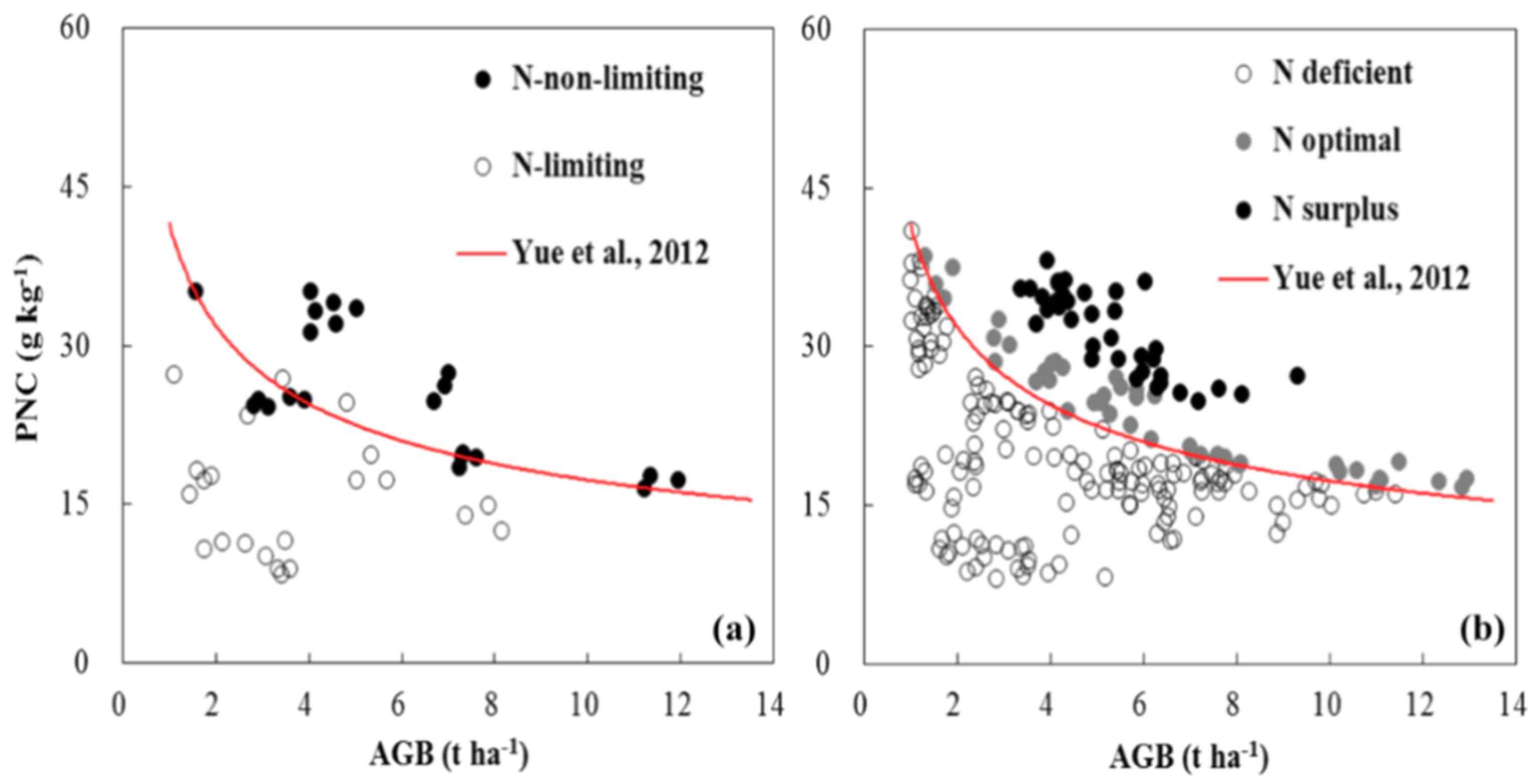
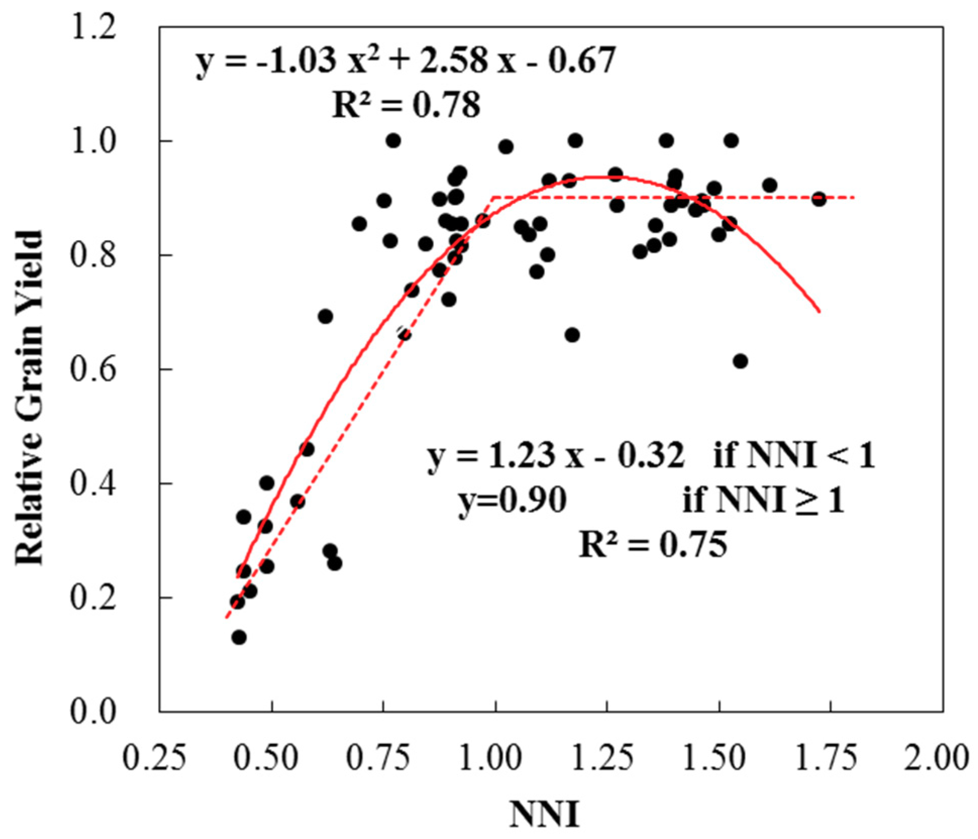
3.2. Evaluation of the Established Critical Nitrogen Dilution Curve

Figure 1a indicated that 91% of N-limiting data points were below the critical N dilution curve and 73% of non-N-limiting data points were above the curve. All experimental data across different N rates, varieties, sites, and years were classified into three categories of N status—N deficient (NNI < 1.00), N optimal (1.00 ≤ NNI ≤ 1.25), and N surplus (NNI > 1.25). The N surplus samples were all above the Nc dilution curve, N deficient samples were all below the curve, and N optimal samples were all on or close to the curve (Figure 1b), which indicated that the published critical N dilution curve and the NNI threshold values were suitable for the study region in NCP.
The relationships between NNI and relative grain yield could be described with a linear plateau model or a quadratic model, with R2 of 0.75 and 0.78, respectively (Figure 2). When 1.00 ≤ NNI ≤ 1.25, based on these relationships, the relative grain yield reached a plateau or a peak. When NNI > 1.25, the relative grain yield began to decrease based on the quadratic model. These results indicated that the NNI thresholds of 1.00 and 1.25 were suitable for the study region.

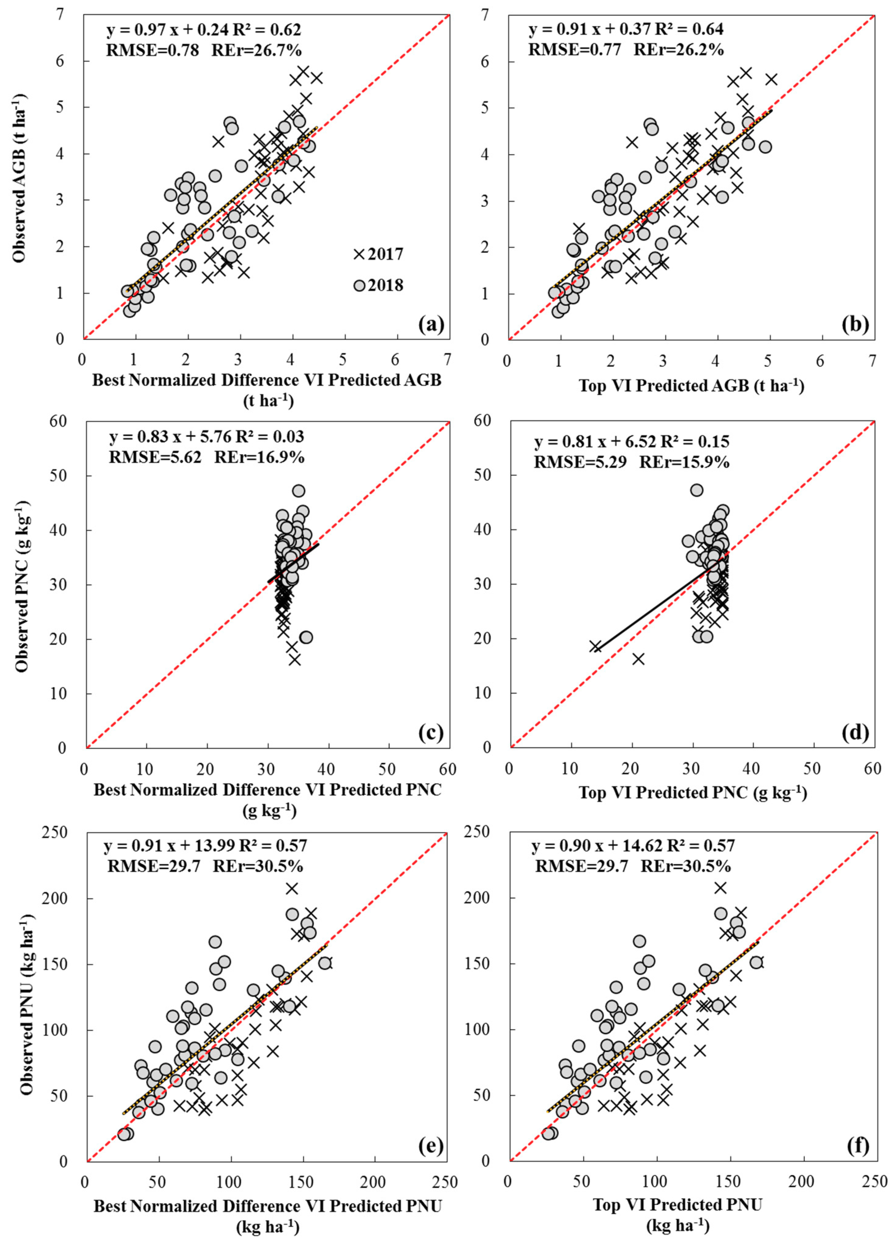
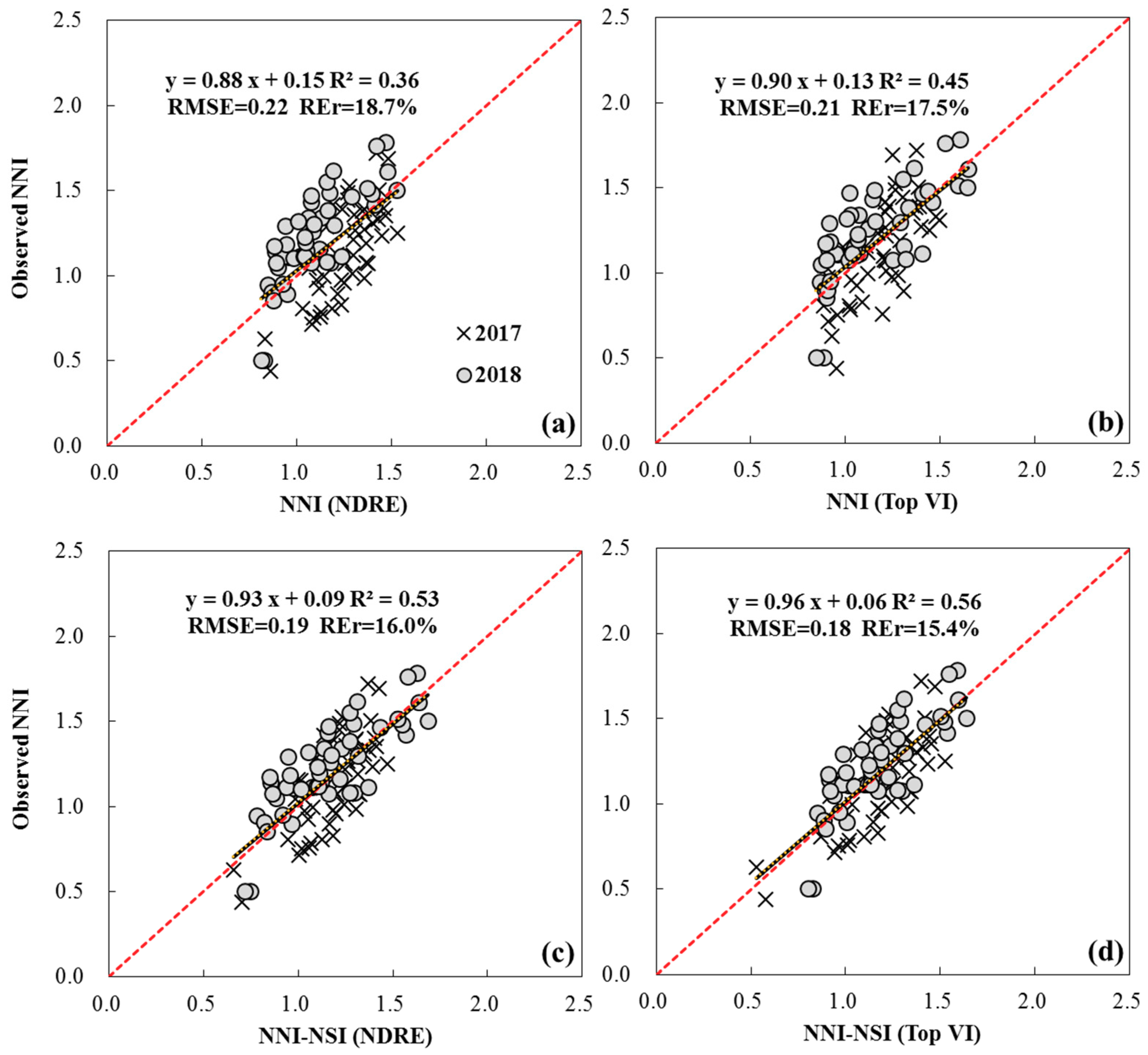
3.3. The Estimation of NNI Using Two Indirect Approaches

The performance of normalized difference VIs and the top three VIs for estimating winter wheat AGB, PNC, and PNU varied across different N rate and management treatments, varieties, and years (Table 2). The top VI, normalized near infrared index (NNIRI), explained 72% of AGB variability across varieties and stages. The normalized difference VIs performed similarly or slightly worse across varieties and years, explaining 62%–70% of AGB variability. The validation results were similar to the calibration results (Figure 3a,b). NDVI and the top VIs had similar performance across varieties and stages for predicting AGB, with R2, RMSE, and REr being 0.62–0.64, 0.77 t ha−1–0.78 t ha−1, and 26.2%–26.7%, respectively.
Modified canopy chlorophyll content index (MCCCI, 15%), plant senescence reflectance index (PSRI, 9%), and green and red difference (GRD, 9%) were chosen as the top three VIs to estimate PNC. Nevertheless, across varieties and years, the association between all VIs and PNC were poor. All normalized difference VIs did not correlate with PNC significantly (1–3%). The validation results were similar to the calibration results (Figure 3c,d). MCCCI and GNDVI did not perform well, with R2, RMSE, and REr being 0.03–0.15, 5.29 g kg−1–5.62 g kg−1, and 15.9–16.9%, respectively.
The top three VIs—Optimized red edge vegetation index (REVIopt), modified red edge simple ratio (MSR_RE), and transformed normalized green and red (TNDGR)—had the best performance for estimating PNU (R2 = 0.64). NDRE (R2 = 0.64) had the same performance as the top VIs. NDVI and GNDVI explained less PNU variability (R2 = 0.46–0.58). The validation results indicated that NDRE also had the same performance as the top VIs (R2 = 0.57) (Figure 3e,f).
Based on the above results, two different indirect approaches (NNI-PNC and NNI-PNU) (see formulas (1), (2), and (3)) were used in this study to estimate NNI and the validation results were shown in Figure 4. The NNI-PNU method (R2 = 0.39) demonstrated slightly better performance than those of NNI-PNC method (R2 = 0.29–0.38) across varieties and years. Regardless of the approach used, the top VI performed slightly better (R2 = 0.38–0.39, RMSE = 0.22–0.23, and REr = 18.6%–19.2%) than the normalized difference VIs (R2 = 0.29–0.39, RMSE = 0.22–0.23, and REr = 18.8%–19.7%).

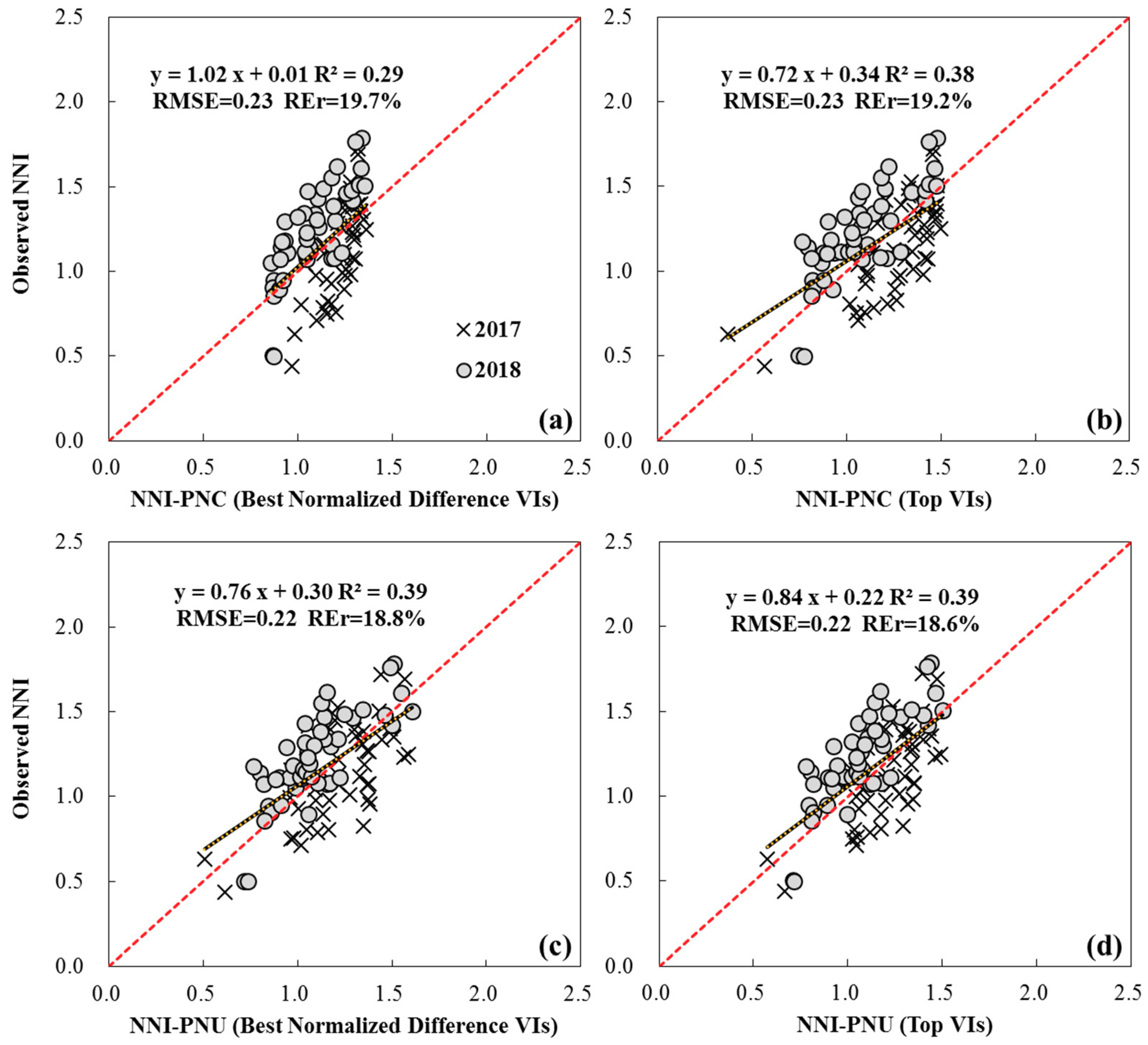
3.4. The Estimation of NNI Using Two Direct Approaches

The relationships between VIs or NSI calculated with VIs (NSI_VIs) and NNI across varieties and years are listed in Table 2. Across the two years, the correlations of all VIs with NNI were not satisfactory (R2 < 0.50). Compared with the VIs, NSI_VIs were more strongly related to NNI. The NSI_VIs (R2 = 0.44–0.57) performed much better than their corresponding original VIs (R2 = 0.20–0.46). NSI calculated from red edge wide dynamic range vegetation index (NSI_REWDRVI), red edge difference vegetation index (NSI_REDVI), and red edge ratio vegetation index (NSI_RERVI) all had the best correlations with NNI (R2 = 0.56–0.57). NSI_NDRE had similar performance for estimating NNI (R2 = 0.52), whereas NSI_NDVI and NSI_GNDVI performed slightly worse (R2 = 0.44) across varieties and years.
The validation results of NNI for these two different direct approaches (NNI-VI and NNI-NSI) using the optimal estimation model of a NDRE, NSI_NDRE, the top VIs (TNDGR), and the top NSI_VI (NSI_REWDRVI) also confirmed this observation (Figure 5). For the NNI-VI approach, the validation results of TNDGR (R2 = 0.45, RMSE = 0.21 and REr = 17.5%) were better than NDRE (R2 = 0.36, RMSE = 0.22 and REr = 18.7%) across varieties and years. For the NNI-NSI approach, there was little difference between NSI_NDRE and NSI_REWDRVI, explaining 53% and 56% variability of NNI, respectively. The top NSI-VI explained slightly more (11%) variability than the top VIs, whereas NSI_NDRE explained 17% more variability in NNI than NDRE.

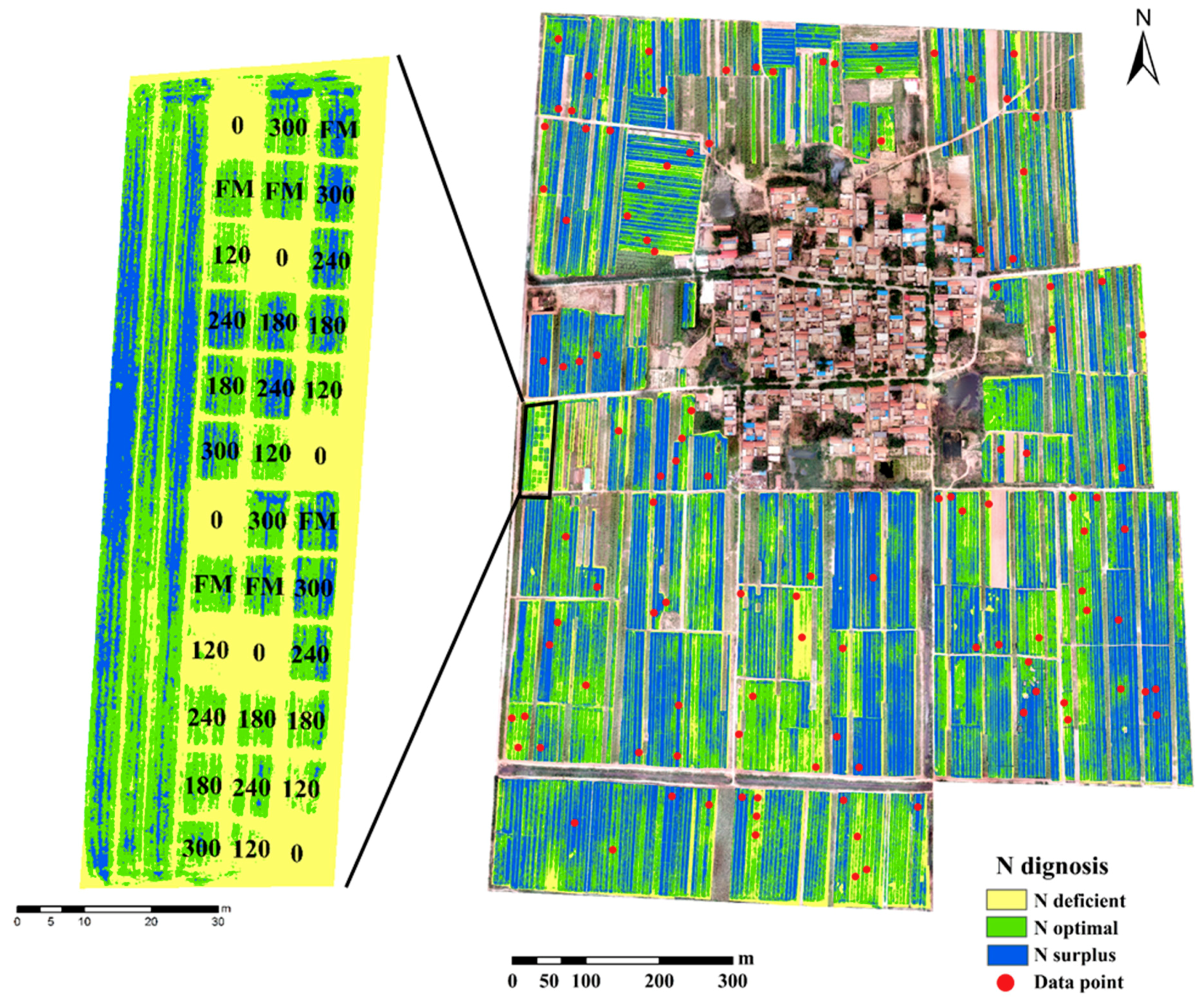
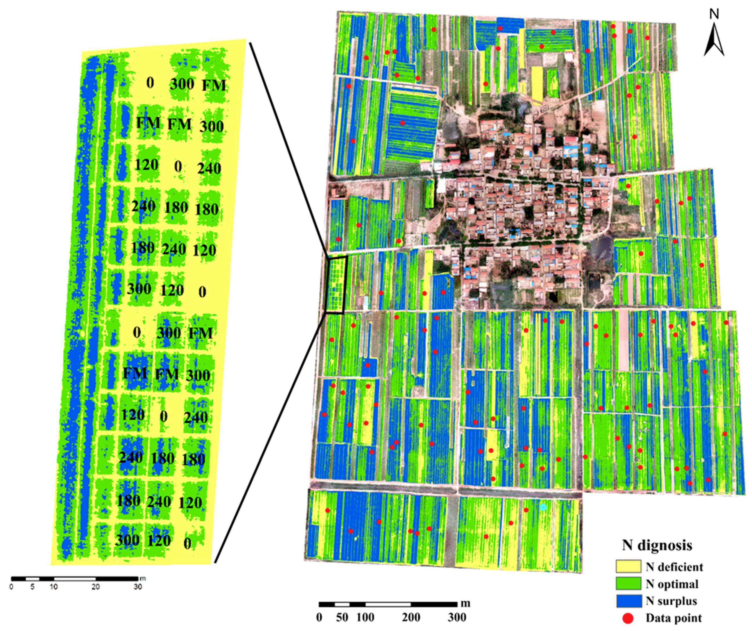
3.5. Nitrogen Status Diagnosis at the Village Scale

To evaluate the diagnostic accuracy of the four different approaches, the calibration and validation dataset was divided into three classes: N deficient, N optimal, and N surplus based on destructively measured NNI and the threshold values proposed in this study (see Methods). The results of the diagnosis using the four different approaches were compared with the measured NNI, and the resulting areal agreement and kappa statistics are listed in Table 3.
The four approaches using the top VIs represent the potential of using eBee UAV-based multispectral remote sensing for winter wheat N status diagnosis. Their accuracies ranged from 52% to 59%, with kappa statistics being 0.28–0.37. The two approaches using VI to estimate NNI directly (57%–59%) gained better accuracy than two indirect approaches (52%–54%). In the two indirect approaches, there was no significant difference between the models established using the normalized difference VIs or the top VIs. In the NNI-VI approach, the top VIs (57%, kappa = 0.34) performed better than normalized difference VIs (53%, kappa = 0.29). The NNI-NSI approach was the most stable approach (57%–59%) and was least influenced by the VIs used. NSI_REWDRVI reached the best accuracy (59%, kappa = 0.37) of all approaches, but NSI_NDRE (57%, kappa = 0.34) had comparable performance.
The N diagnosis maps created using the NNI-NSI approach for the village’s fields in 2017 and 2018 are shown in Figure 6 and Figure 7 at the pixel level. In 2017, most of the farmer fields were well- or over-fertilized, falling into the surplus N status category. In contrast, in 2018, there was a large variation of winter wheat N status in farmer fields, and more fields were diagnosed as N deficient. In both growing seasons, the spectral images of the N experiments displayed a varying crop performance induced by the ranging N rates as well as variable soil and growing conditions.

4. Discussion

Using fixed-wing UAV remote sensing to estimate plant NNI for diagnosing winter wheat N status and guiding in-season site-specific N management at the village scale is an attractive idea. Before practical applications of this technology can be implemented, several questions need to be answered— (1) How accurately can this system diagnose winter wheat N status at a village-scale? (2) Will the commonly used normalized difference VIs be good enough for wheat N status diagnosis before N topdressing application? (3) Which NNI estimation approach should be used for wheat N status diagnosis? (4) Will the suitable VI and NNI estimation approach be satisfactory for small scale-farming and practical for guiding in-season site-specific N management in NCP? This research was conducted in order to address these questions.

4.1. The Accuracy of N Status Diagnosis Using eBee UAV Remote Sensing

The results of this study indicated that the diagnostic accuracy obtained with eBee UAV-based multispectral sensor varied with NNI estimation approaches used. The two direct methods of using VI to estimate NNI directly (57%–59%) achieved better diagnostic accuracy than two indirect approaches (52%–54%) across varieties and years. So far, no similar study has been conducted to show the potential of N diagnosis using UAV remote sensing. For winter wheat, several studies indicated an acceptable applicability of VIs for estimating NNI directly or indirectly. Chen [30] obtained good validation results of estimating NNI indirectly (R2 = 0.85–0.89, RMSE = 0.11–0.13) and directly (R2 = 0.81–0.88, RMSE = 0.11–0.31) across all growth stages using Analytical Spectral Devices (ASD) spectroradiometer. Cao et al. [41] found green re-normalized difference vegetation index (GRDVI, R2 = 0.78) and modified green soil adjusted vegetation index (MGSAVI, R2 = 0.77)) using Crop Circle ACS-470 sensor performed consistently better than GreenSeeker NDVI (R2 = 0.47) and RVI (R2 = 0.44) for estimating NNI directly. Cao et al. [42] found good performance for estimating NNI directly with NDRE obtained from Crop Circle ACS-430 (R2 = 0.84–0.89) and Crop Circle ACS-470 (R2 = 0.71–0.86) and achieved substantial agreement (69%–74%) for N diagnosis at suitable height of sensor over crop canopy across growth stages. The abovementioned results were more accurate than the results obtained in this study. It should be noted that all the previous studies used data from small plot experiments and ground canopy sensors. N plot experiments can be used to determine crop growth information under different N effects by actual sampling or remote sensing. However, it is not sufficient to apply the model from N plot experiments to a larger area (e.g., across a village) because there are many factors that may potentially limit crop growth in smallholder farmer fields. It is necessary to sample biomass and measure crop N status both in plot experiments and in farmer fields to further determine the modeling accuracy at village scale. In this study, the samples were collected from several N plot experiments and different smallholder farmer fields across the whole village, including many confounding factors due to different farmers’ management practices such as varieties, sowing dates, planting densities, and fertilizer rates, etc. These factors can decrease the performance of direct NNI estimation [30,31], but they contribute to the true representation of the actual situation in smallholder farmer fields.
Moreover, in the previous studies, most of the well-fitted relationships were observed at late crop growth stages. This study was performed at Feekes 6, which is the stem elongation stage of winter wheat and the key stage for N topdressing. At early growth stages, AGB increases faster than PNU and dominates the canopy reflectance, which may be considered a reason for not obtaining good relationships with PNC and NNI in this study. Lu et al. [31] also reported unsatisfactory results on estimating PNC (R2 = 0.22) and NNI (R2 = 0.42) using RapidSCAN sensor at early growth stages (panicle initiation and stem elongation stages) in rice from 16 plot experiments and 10 on-farm experiments.

4.2. The Performance of Normalized Difference VIs

The normalized difference VIs are acceptable for wheat N status diagnosis without the need of searching for other indices. Although using the top VIs (R2 = 0.15 and 0.46) significantly improved the prediction of PNC and NNI compared to using normalized difference VIs (R2 = 0.03 and 0.39), using NDVI and NDRE could have similar performance as the top VIs in the prediction of AGB (R2 = 0.70 vs. R2 = 0.72) and PNU (R2 = 0.64 vs. R2 = 0.64), respectively. The NNI-NSI approach using N rich plots to eliminate some confounding factors, by incorporation NDRE index, achieved comparable good performance (areal agreement = 57%, kappa = 0.34) with the top VIs (areal agreement = 59%, kappa = 0.37). One of the main reasons for the superior performance of NDRE might be that the red-edge band is more sensitive to crop N status than the red and infrared bands included in the NDVI [41,42,43]. Moreover, the performance of the NDVI is also limited by variation between fields [44]. Calculating NSI improved the ability of crop N diagnosis, which was in agreement with Lu et al. [31] and Lu et al. [45] (areal agreement = 59%, kappa = 0.38). This is an encouraging finding, which would let us simplify both in-field practices as well as image processing and diagnostic calculations, making the use of fixed-wing UAV in agricultural practice more straightforward.

4.3. The Suitability and Usability of the NNI Estimation Approach

Which approach of N status diagnosis is most accurate and stable? The indirect approaches might be very promising for indirect NNI estimation, which was recommended by Chen [30], Xia et al. [32], and Huang et al. [17] for winter wheat, maize, and rice, respectively. However, the indirect approaches used in this study did not achieve promising diagnostic accuracy regardless of which VIs were used (areal agreement < 54%). One of the reasons may be the unsatisfactory performance of UAV remote sensing for estimating PNC (R2 < 0.15) or PNU (R2 < 0.64) across smallholder fields when compared with the abovementioned studies. It is a big challenge to reliably estimate PNC or PNU across diverse smallholder fields. Bonfil [44] indicated that a wrong decision can be made if N is not the limiting factor that retards biomass production. Zhang et al. [5] reported that yield-limiting factors in NCP are very complex, involving agronomic, infrastructural, and socioeconomic issues, and most farmer fields show surplus crop N status. Cao et al. [8] calculated indigenous N supply (INS) and found INS varied significantly both within individual fields and across different fields, ranging from 33.4 to 268.4 kg N ha−1. In future research and practical applications, variables additional to crop sensing data such as soil spatial variation and crop managements should be included to improve the large-scale crop N diagnosis models.
Chen [30] indicated that the direct approach was more influenced by growth stages, which is in agreement with this study. The dataset included only one stage but spanned over two years. The NNI-VI approach used in this study resulted in fair areal agreement (53–57%). A promising approach to overcome the influence of phenology or other stress factors is to use the NSI or response index approach, which uses an N rich plot or strip as a reference to normalize the VIs [32,33]. Xia et al. [32] found out that using NDVI to calculate response index (RI) and then estimate NNI for diagnosing maize N status was similar to or more accurate and stable (areal agreement = 71–76%) than the indirect approaches and the NNI-VI direct approach. Lu et al. [31] reported that the NNI-NSI approach was very stable (areal agreement = 59–76%) across growth stages, varieties, and site-years, without being influenced significantly by the VIs used for rice. In this study, the NNI-NSI approach also achieved the most stable diagnostic accuracy (57%–59%), regardless of which VI was used. Using NSI thresholds to diagnose N status directly was also quite stable and simple for practical applications. Xia et al. [32] found that the approach using RI calculated with NDVI to directly diagnose maize N status performed best among the five approaches tested in their study. Therefore, the NNI-NSI approach should be recommended for winter wheat N status diagnosis at village-scale using eBee UAV remote sensing.

4.4. Applications for N Status Diagnosis and Topdressing N Recommendation

After the diagnosis of the crop N status in farmer fields, it is more important to determine how much N fertilizer is needed for each field. The NNI-based crop N status map can be used to guide in-season topdressing N application [17]. The first method is to adjust N rates based on N status categories. For example, for the optimal N category or zone, the regional optimum topdressing N application rate of 138 kg N ha−1 can be applied. This rate can be increased or decreased by a certain level if the winter wheat N status is deficient or surplus. This method is commonly used in site-specific N management of rice based on chlorophyll meter diagnosis developed by the International Rice Research Institute [46]. It is empirical, but quite practical for on-farm applications in small-scale farming systems. A quantitative NNI-based method proposed by Huang et al. [17] is to produce a PNU difference map using the estimated PNU map minus the PNUc map or PNUc × (NNI-1). PNUc can be calculated by estimated AGB multiplied by Nc. The recommended N topdressing application rate can be determined using the regional optimum topdressing N rate minus the PNU difference [17]. The third method is to recommend N rates based on the Modified Green Window Approach [12] or Ramp Calibration Strips strategy and UAV remote sensing. Raun et al. [47] proposed Ramp Calibration Strip Technology for determining midseason N rates in corn and wheat based on NDVI from canopy sensor. Yue et al. [34] developed the Green Window Approach and increased wheat yield, apparent N recovery, net economic benefits by 13%, 76% and 60% in NCP, respectively. Cao et al. [12] used the Modified Green Window-based strategy to guide N management of winter wheat-summer maize rotation system and achieved better results than regional optimum N management (RONM) for summer maize, but similar results as RONM for winter wheat in NCP. Studies are needed to evaluate these different approaches at the village scale.
There were several challenges for using N diagnosis and topdressing N recommendation at village scale. This study used the high N-rate plots in the field experiments as N rich plots. One set of N rate plots for the whole village may not be sufficient to produce reliable recommendations. Roberts et al. [48] found that the Ramp Calibration Strips approach did not work well in large U.S. winter wheat fields. In the NCP, the soil fertility conditions have significant field-to-field variability due to the fact that the farmer fields are very small, and the crop management is different from farmer to farmer [8]. Therefore, one calibration or N rich plot in each field would be ideal but is not practical. One alternative is to delineate all the fields in a village into a few relatively uniform management zones [49]. Then, a single N rich plot or a set of Ramp Calibration Strips can be established in each management unit. More studies are needed to further evaluate such strategies under on-farm conditions in small farming systems to determine their potential to improve NUE as compared with current farmer management practices or regional optimum management.

5. Conclusions

This study evaluated the potential of using eBee UAV-based multispectral remote sensing to estimate winter wheat NNI at the Feekes 6 stage (stem elongation) for guiding topdressing N application in small farming systems of NCP. The top VIs of the eBee UAV remote sensing were significantly related to AGB (R2 = 0.70–0.72) and PNU (R2 = 0.64) across fields, varieties, and years. The best VI achieved an estimation accuracy of 59% for N status diagnosis at stem elongation stage of winter wheat. The most practical and stable method was using VIs to calculate NSI and then to non-destructively estimate NNI (R2 = 0.53–0.56). The approach using NSI thresholds to diagnose N status directly was quite stable and simple for practical applications, with 57–59% diagnostic accuracy rate. This approach was the least affected by the VIs used to calculate NNI across fields, varieties, and years. Moreover, the calculated difference between the estimated PNU and the critical PNU can be used to adjust the topdressing N application rates. This study demonstrated that the eBee fixed-wing UAV remote sensing system had a great potential to be used in estimating N status of winter wheat for guiding N topdressing application in smallholder farming systems at a village scale in NCP. More studies are needed to further develop and evaluate fixed-wing UAV remote sensing–based precision N management strategies in small farming systems.

Author Contributions

Conceptualized and designed the research, Y.M. and Z.C.; performed the field experiments and data collection, Z.C., L.Z., Y.L., W.L., and Z.Z.; analyzed the data, Z.C. and J.L.; wrote the original manuscript, Z.C.; reviewed and revised the paper, J.L., Y.M., and K.K. The research was supervised by Y.M., H.Z., and C.L. Y.M. and K.K. secured the research funding and managed the projects.

Funding

This research was funded by the National Basic Research Program of China (2015CB150405), and Norwegian Ministry of Foreign Affairs (SINOGRAIN II, CHN-17/0019).

Acknowledgments

The authors thank Jun Liang at Laoling County Bureau of Agriculture in Shandong Province for their assistance during this research. We also would like to thank all of the farmers for their cooperation in this research, and reviewers for their suggestions to improve the manuscript.

Conflicts of Interest

The authors declare no conflict of interest.

Appendix A

Table A1. The vegetation indices evaluated in this study. G, R, RE, and NIR indicate green, red, red edge, and near infrared band reflectance.
IndexFormulaReference
Normalized Difference Vegetation Index (NDVI)(NIR − R)/(NIR + R)[50]
Ratio Vegetation Index (RVI)NIR/R[51]
Difference Vegetation Index (DVI)NIR − R[52]
Renormalized Difference Vegetation Index (RDVI)(NIR − R)/SQRT (NIR + R)[53]
Wide Dynamic Range Vegetation Index (WDRVI)(0.12 × NIR − R)/(0.12 × NIR + R)[54]
Soil Adjusted Vegetation Index (SAVI)1.5 × (NIR − R)/(NIR + R + 0.5)[55]
Optimized SAVI (OSAVI)(1 + 0.16) × (NIR − R)/(NIR + R + 0.16)[56]
Modified SAVI (MSAVI)0.5 × [2 × NIR + 1 − SQRT ((2 × NIR + 1)2 − 8 × (NIR − R))][57]
Modified Simple Ratio (MSR)(NIR/R − 1)/SQRT (NIR/R + 1)[58]
Transformed Normalized vegetation index (TNDVI)SQRT ((NIR − R)/(NIR + R) + 0.5)[59]
Optimal Vegetation Index (VIopt)1.45 × ((NIR2 + 1)/(R + 0.45)) [60]
Red Edge Point Reflectance (REPR)(R + NIR)/2[61]
Nonlinear Index (NLI)(NIR2 − R)/(NIR2 + R)[62]
Modified Nonlinear Index (MNLI)1.5 × (NIR2 − R)/(NIR2 + R + 0.5)[63]
NDVI*RVI(NIR2 − R)/(NIR + R2)[63]
SAVI*SR(NIR2 − R)/((NIR + R + 0.5) × R)[63]
Normalized Difference Red Edge (NDRE)(NIR − RE)/(NIR + RE)[64]
Red Edge Ratio Vegetation Index (RERVI)NIR/RE[65]
Red Edge Difference Vegetation Index (REDVI)NIR − RE[66]
Red Edge Renormalized Different Vegetation Index (RERDVI)(NIR − RE)/SQRT (NIR + RE)[66]
Red Edge Wide Dynamic Range Vegetation Index (REWDRVI)(0.12 × NIR − RE)/(0.12 × NIR + RE)[66]
Red Edge Soil Adjusted Vegetation Index (RESAVI)1.5 × (NIR − RE)/(NIR + RE + 0.5)[66]
Red Edge Optimized SAVI (REOSAVI)(1 + 0.16) × (NIR − RE)/(NIR + RE + 0.16)[66]
Modified Red Edge SAVI (MRESAVI)0.5 × (2 × NIR + 1 − SQRT ((2 × NIR + 1)2 − 8 × (NIR − RE)))[66]
Modified Red Edge Simple Ratio (MSR_RE)(NIR/RE − 1)/SQRT (NIR/RE + 1)[66]
Optimized Red Edge Vegetation Index (REVIopt)100 × (lnNIR − lnRE)[67]
Green Normalized Difference Vegetation Index (GNDVI)(NIR − G)/(NIR + G)[68]
Green Ratio Vegetation Index (GRVI)NIR/G[69]
Green Difference Vegetation Index (GDVI)NIR − G[17]
Green Renormalized Difference Vegetation Index (GRDVI)(NIR − G)/SQRT (NIR + G)[17]
Green Wide Dynamic Range Vegetation Index (GWDRVI)(0.12 × NIR − G)/(0.12 × NIR + G)[17]
Green Soil Adjusted Vegetation Index (GSAVI)1.5 × (NIR − G)/(NIR + G + 0.5)[17]
Green Optimized SAVI (GOSAVI)(1 + 0.16) × (NIR − G)/(NIR + G + 0.16)[17]
Modified Green SAVI (MGSAVI)0.5 × (2 × NIR + 1 − SQRT ((2 × NIR + 1)2 − 8 × (NIR − G)))[17]
Modified Green Simple Ratio (MSR_G)(NIR/G − 1)/SQRT (NIR/G + 1)[66]
Red Edge Normalized Difference Vegetation Index (RENDVI)(RE − R)/(RE + R)[70]
Red Edge Simple Ratio (RESR)RE/R[71]
Modified Red Edge Difference Vegetation Index (MREDVI)RE − RThis study, modified from [52]
Modified Simple Ratio Green and Red (MSRGR)SQRT(G/R)[52]
Green and Red Difference (GRD)G − R[52]
Normalized Difference Green and Red (NDGR)(G − R)/(G + R)[52]
Greenness Index (GI)G/R[52]
Transformed Normalized Green and Red (TNDGR)SQRT ((G − R)/(G + R) + 0.5)[52]
MERIS terrestrial chlorophyll index (MTCI)(NIR − RE)/(RE − R)[61]
DATT index (DATT)(NIR − RE)/(NIR − R)[72]
Modified canopy chlorophyll content index (MCCCI)NDRE/NDVI[73]
Modified Normalized Difference Vegetation Index 1 (mNDVI1)(NIR − R + 2 × G)/(NIR + R − 2 × G)[74]
Plant Senescence Reflectance Index (PSRI)(R − G)/NIR[75]
Modified Chlorophyll Absorption in Reflectance Index (MCARI)((RE − R) − 0.2 × (RE − G)) × (RE/R)This study, modified from [76]
Modified Chlorophyll Absorption in Reflectance Index 1 (MCARI1)1.2 × [2.5 × (NIR−R) − 1.3 × (NIR − G)][77]
Modified Chlorophyll Absorption in Reflectance Index 2 (MCARI2)1.5 × (2.5 × (NIR − R) − 1.3 × (NIR − G)) /SQRT ((2 × NIR + 1)2 − (6 × NIR − 5 × SQRT(R)) − 0.5)[77]
Triangular Vegetation Index (TVI)0.5 × (120 × (NIR − G) − 200 × (R − G)][78]
Transformed Chlorophyll Absorption in Reflectance Index (TCARI)3 × ((RE − R) − 0.2 × (RE − G) × (RE/R))This study, modified from [79]
Triangular Chlorophyll Index (TCI)1.2 × (RE − G) − 1.5 × (R − G) × SQRT (RE/R)This study, modified from [80]
TCARI/OSAVITCARI/OSAVI[79]
TCARI/MSAVITCARI/MSAVI[79]
TCI/OSAVITCI/OSAVI[80]
Normalized Near Infrared Index (NNIRI)NIR/(NIR + RE + R)[31]
Red Edge Transformed Vegetation Index (RETVI)0.5 × (120 × (NIR − R) − 200 × (RE − R))[31]
Table A2. Abbreviations used in this paper.
AbbreviationFull NameAbbreviationFull Name
AGBaboveground biomassNSI_NDREnitrogen sufficiency index calculated with normalized difference red edge
ASDanalytical spectral devicesNSI_NDVInitrogen sufficiency index calculated with normalized difference vegetation index
CVcoefficient of variationNSI_REDVInitrogen sufficiency index calculated with red edge difference vegetation index
DMdry matterNSI_RERVInitrogen sufficiency index calculated with red edge ratio vegetation index
Eexponential fitNSI_REWDRVInitrogen sufficiency index calculated with red edge wide dynamic range vegetation index
FMfarmer managementNSI_VIsnitrogen sufficiency index calculated with vegetation indices
GgreenNUEnitrogen use efficiency
GNDVIgreen normalized difference vegetation indexPpower fit
GRDgreen and red differencePNCplant nitrogen concentration
GRDVIgreen renormalized difference vegetation indexPNMprecision nitrogen management
INSindigenous nitrogen supplyPNUplant nitrogen uptake
KClpotassium chloridePNUaactual measured plant nitrogen uptake
MCCCImodified canopy chlorophyll content indexPNUccritical plant nitrogen uptake
MGSAVImodified green soil adjusted vegetation indexPSRIplant senescence reflectance index
MSR_REmodified red edge simple ratioQquadratic fit
NnitrogenRred
Naactual measured nitrogen concentrationREred edge
Nccritical nitrogen concentrationREIPred-edge inflection point
NCPNorth China PlainRErrelative error
NDREnormalized difference red edgeREVIoptoptimized red edge vegetation index
NDVInormalized difference vegetation indexREWDRVIred edge wide dynamic range vegetation index
NIRnear infraredRMSEroot mean square error
Nminmineral nitrogenSDstandard deviation of the mean
NNInitrogen nutrition indexTNDGRtransformed normalized green and red
NNIRInormalized near infrared indexUAVunmanned aerial vehicle
NSInitrogen sufficiency indexVIsvegetation indices
NSI_GNDVInitrogen sufficiency index calculated with green normalized difference vegetation index

References

  1. Wang, J.; Wang, E.; Yang, X.; Zhang, F.; Yin, H. Increased yield potential of wheat-maize cropping system in the North China Plain by climate change adaptation. Clim. Chang. 2012, 113, 825–840. [Google Scholar] [CrossRef]
  2. Cui, Z.; Zhang, H.; Chen, X.; Zhang, C.; Ma, W.; Huang, C.; Zhang, W.; Mi, G.; Miao, Y.; Li, X. Pursuing sustainable productivity with millions of smallholder farmers. Nature 2018, 555, 363–366. [Google Scholar] [CrossRef] [PubMed]
  3. Miao, Y.; Stewart, B.A.; Zhang, F. Long-term experiments for sustainable nutrient management in China. A review. Agron. Sustain. Dev. 2011, 31, 397–414. [Google Scholar] [CrossRef]
  4. Chen, G.; Cao, H.; Liang, J.; Ma, W.; Guo, L.; Zhang, S.; Jiang, R.; Zhang, H.; Goulding, K.W.T.; Zhang, F. Factors affecting nitrogen use efficiency and grain yield of summer maize on smallholder farms in the North China Plain. Sustainability 2018, 10, 363. [Google Scholar] [CrossRef]
  5. Zhang, W.; Cao, G.; Li, X.; Zhang, H.; Wang, C.; Liu, Q.; Chen, X.; Cui, Z.; Shen, J.; Jiang, R.; et al. Closing yield gaps in China by empowering smallholder farmers. Nature 2016, 537, 671–674. [Google Scholar] [CrossRef] [PubMed]
  6. Chen, X.; Cui, Z.; Fan, M.; Vitousek, P.; Zhao, M.; Ma, W.; Wang, Z.; Zhang, W.; Yan, X.; Yang, J. Producing more grain with lower environmental costs. Nature 2014, 514, 486–489. [Google Scholar] [CrossRef]
  7. Zhang, F.; Chen, X.; Vitousek, P. Chinese agriculture: An experiment for the world. Nature 2013, 497, 33–35. [Google Scholar] [CrossRef] [PubMed]
  8. Cao, Q.; Cui, Z.; Chen, X.; Khosla, R.; Dao, T.H.; Miao, Y. Quantifying spatial variability of indigenous nitrogen supply for precision nitrogen management in small scale farming. Precis. Agric. 2012, 13, 45–61. [Google Scholar] [CrossRef]
  9. Diacono, M.; Rubino, P.; Montemurro, F. Precision nitrogen management of wheat. A review. Agron. Sustain. Dev. 2013, 33, 219–241. [Google Scholar] [CrossRef]
  10. Miao, Y.; Mulla, D.J.; Hernandez, J.A.; Wiebers, M.; Robert, P.C. Potential impact of precision nitrogen management on corn yield, protein content, and test weight. Soil Sci. Soc. Am. J. 2007, 71, 1490–1499. [Google Scholar] [CrossRef]
  11. Cui, Z.; Zhang, F.; Chen, X.; Miao, Y.; Li, J.; Shi, L.; Xu, J.; Ye, Y.; Liu, C.; Yang, Z.; et al. On-farm evaluation of an in-season nitrogen management strategy based on soil Nmin test. Field Crops Res. 2008, 105, 48–55. [Google Scholar] [CrossRef]
  12. Cao, Q.; Miao, Y.; Feng, G.; Gao, X.; Liu, B.; Liu, Y.; Li, F.; Khosla, R.; Mulla, D.; Zhang, F. Improving nitrogen use efficiency with minimal environmental risks using an active canopy sensor in a wheat-maize cropping system. Field Crops Res. 2017, 214, 365–372. [Google Scholar] [CrossRef]
  13. Yao, Y.; Miao, Y.; Huang, S.; Gao, L.; Ma, X.; Zhao, G.; Jiang, R.; Chen, X.; Zhang, F.; Yu, K. Active canopy sensor-based precision N management strategy for rice. Agron. Sustain. Dev. 2012, 32, 925–933. [Google Scholar] [CrossRef] [Green Version]
  14. Huang, S.; Miao, Y.; Yuan, F.; Gnyp, M.; Yao, Y.; Cao, Q.; Wang, H.; Lenzwiedemann, V.; Bareth, G. Potential of Rapideye and Worldview-2 satellite data for improving rice nitrogen status monitoring at different growth stages. Remote Sens. 2017, 9, 227. [Google Scholar] [CrossRef]
  15. Zhao, Q.; Lenzwiedemann, V.I.S.; Yuan, F.; Jiang, R.; Miao, Y.; Zhang, F.; Bareth, G. Investigating within-field variability of rice from high resolution satellite imagery in Qixing Farm County, Northeast China. ISPRS Int. J. Geo-Inf. 2015, 4, 236–261. [Google Scholar] [CrossRef]
  16. Gevaert, C.M.; Suomalainen, J.; Tang, J.; Kooistra, L. Generation of spectral–temporal response surfaces by combining multispectral satellite and hyperspectral UAV imagery for precision agriculture applications. IEEE J. Sel. Top. Appl. Earth Obs. Remote Sens. 2015, 8, 3140–3146. [Google Scholar] [CrossRef]
  17. Huang, S.; Miao, Y.; Zhao, G.; Yuan, F.; Ma, X.; Tan, C.; Yu, W.; Gnyp, M.L.; Lenz-Wiedemann, V.I.; Rascher, U. Satellite remote sensing-based in-season diagnosis of rice nitrogen status in Northeast China. Remote Sens. 2015, 7, 10646–10667. [Google Scholar] [CrossRef]
  18. Yang, G.; Liu, J.; Zhao, C.; Li, Z.; Huang, Y.; Yu, H.; Xu, B.; Yang, X.; Zhu, D.; Zhang, X. Unmanned aerial vehicle remote sensing for field-based crop phenotyping: Current status and perspectives. Front. Plant Sci. 2017, 8, 1111. [Google Scholar] [CrossRef]
  19. Geipel, J.; Link, J.; Wirwahn, J.; Claupein, W. A programmable aerial multispectral camera system for in-season crop biomass and nitrogen content estimation. Agriculture 2016, 6, 4. [Google Scholar] [CrossRef]
  20. Perry, E.M.; Goodwin, I.; Cornwall, D. Remote sensing using canopy and leaf reflectance for estimating nitrogen status in red-blush pears. Hortscience 2018, 53, 78–83. [Google Scholar] [CrossRef]
  21. Zheng, H.; Cheng, T.; Li, D.; Yao, X.; Tian, Y.; Cao, W.; Zhu, Y. Combining unmanned aerial vehicle (UAV)-based multispectral imagery and ground-based hyperspectral data for plant nitrogen concentration estimation in rice. Front. Plant Sci. 2018, 9, 936. [Google Scholar] [CrossRef] [PubMed]
  22. Yin, X.; Huang, M.; Zou, Y.; Jiang, P.; Cao, F.; Xie, X. Chlorophyll meter-based nitrogen management for no-till direct seeded rice. Res. Crop. 2012, 13, 809–821. [Google Scholar]
  23. Marcaccio, J.V.; Markle, C.E.; Chow-Fraser, P. Use of fixed-wing and multi-rotor unmanned aerial vehicles to map dynamic changes in a freshwater marsh. J. Unmanned Veh. Syst. 2016, 4, 193–202. [Google Scholar] [CrossRef]
  24. Roumenina, E.; Jelev, G.; Dimitrov, P.; Vassilev, V.; Krasteva, V.; Kamenova, I.; Nankov, M.; Kolchakov, V. Winter Wheat Crop State Assessment, Based on Satellite Data from the Experiment Spot-5 Take-5, Unmanned Airial Vehicle Sensefly Ebee Ag and Field Data in Zlatia Test Site, Bulgaria. In Proceedings of the Eleventh Scientific Conference with International Participation, Sofia, Bulgaria, 4–6 November 2015. [Google Scholar]
  25. Marino, S.; Alvino, A. Detection of homogeneous wheat areas using multi-temporal UAS images and ground truth data analyzed by cluster analysis. Eur. J. Remote Sens. 2018, 51, 266–275. [Google Scholar] [CrossRef] [Green Version]
  26. Greenwood, D.J.; Gastal, F.; Lemaire, G.; Draycott, A.; Millard, P.; Neeteson, J.J. Growth rate and % N of field grown crops: Theory and experiments. Ann. Bot. 1991, 67, 181–190. [Google Scholar] [CrossRef]
  27. Lemaire, G.; Jeuffroy, M.-H.; Gastal, F. Diagnosis tool for plant and crop N status in vegetative stage: Theory and practices for crop N management. Eur. J. Agron. 2008, 28, 614–624. [Google Scholar] [CrossRef]
  28. Yuan, Z.; Ata-Ul-Karim, S.T.; Cao, Q.; Lu, Z.; Cao, W.; Zhu, Y.; Liu, X. Indicators for diagnosing nitrogen status of rice based on chlorophyll meter readings. Field Crops Res. 2016, 185, 12–20. [Google Scholar] [CrossRef]
  29. Zhao, B.; Liu, Z.; Ata-Ul-Karim, S.T.; Xiao, J.; Liu, Z.; Qi, A.; Ning, D.; Nan, J.; Duan, A. Rapid and nondestructive estimation of the nitrogen nutrition index in winter barley using chlorophyll measurements. Field Crops Res. 2016, 185, 59–68. [Google Scholar] [CrossRef]
  30. Chen, P. A comparison of two approaches for estimating the wheat nitrogen nutrition index using remote sensing. Remote Sens. 2015, 7, 4527–4548. [Google Scholar] [CrossRef]
  31. Lu, J.; Miao, Y.; Shi, W.; Li, J.; Yuan, F. Evaluating different approaches to non-destructive nitrogen status diagnosis of rice using portable RapidSCAN active canopy sensor. Sci. Rep. 2017, 7, 14073. [Google Scholar] [CrossRef]
  32. Xia, T.; Miao, Y.; Wu, D.; Shao, H.; Khosla, R.; Mi, G. Active optical sensing of spring maize for in-season diagnosis of nitrogen status based on nitrogen nutrition index. Remote Sens. 2016, 8, 605. [Google Scholar] [CrossRef]
  33. Samborski, S.M.; Tremblay, N.; Fallon, E. Strategies to make use of plant sensors-based diagnostic information for nitrogen recommendations. Agron. J. 2009, 101, 800–816. [Google Scholar] [CrossRef]
  34. Yue, X.L.; Hu, Y.; Zhang, H.Z.; Schmidhalter, U. Green Window Approach for improving nitrogen management by farmers in small-scale wheat fields. J. Agric. Sci. 2015, 153, 446–454. [Google Scholar] [CrossRef]
  35. Zhou, X.; Zheng, H.; Xu, X.; He, J.; Ge, X.; Yao, X.; Cheng, T.; Zhu, Y.; Cao, W.; Tian, Y. Predicting grain yield in rice using multi-temporal vegetation indices from UAV-based multispectral and digital imagery. ISPRS J. Photogramm. 2017, 130, 246–255. [Google Scholar] [CrossRef]
  36. Yue, S.; Meng, Q.; Zhao, R.; Li, F.; Chen, X.; Zhang, F.; Cui, Z. Critical nitrogen dilution curve for optimizing nitrogen management of winter wheat production in the North China Plain. Agron. J. 2012, 104, 523–529. [Google Scholar] [CrossRef]
  37. Huang, S.; Miao, Y.; Cao, Q.; Yao, Y.; Zhao, G.; Yu, W.; Shen, J.; Kang, Y.; Bareth, G. A new critical nitrogen dilution curve for rice nitrogen status diagnosis in Northeast China. Pedosphere 2018, 28, 814–822. [Google Scholar] [CrossRef]
  38. Ziadi, N.; Bélanger, G.; Claessens, A.; Lefebvre, L.; Cambouris, A.N.; Tremblay, N.; Nolin, M.C.; Parent, L.É. Determination of a critical nitrogen dilution curve for spring wheat. Agron. J. 2010, 102, 241–250. [Google Scholar] [CrossRef]
  39. Campbell, J.B. Introduction to Remote Sensing, 3rd ed.; The Guilford Press: New York, NY, USA, 2002. [Google Scholar]
  40. Landis, J.R.; Koch, G.G. The measurement of observer agreement for categorical data. Biometrics 1977, 33, 159–174. [Google Scholar] [CrossRef]
  41. Cao, Q.; Miao, Y.; Feng, G.; Gao, X.; Li, F.; Liu, B.; Yue, S.; Cheng, S.; Ustin, S.L.; Khosla, R. Active canopy sensing of winter wheat nitrogen status: An evaluation of two sensor systems. Comput. Electron. Agric. 2015, 112, 54–67. [Google Scholar] [CrossRef]
  42. Cao, Q.; Miao, Y.; Shen, J.; Yuan, F.; Cheng, S.; Cui, Z. Evaluating two crop circle active canopy sensors for in-season diagnosis of winter wheat nitrogen status. Agronomy 2018, 8, 201. [Google Scholar] [CrossRef]
  43. Li, S.; Ding, X.; Kuang, Q.; Ata-Ul-Karim, S.T.; Cheng, T.; Liu, X.; Tian, Y.; Zhu, Y.; Cao, W.; Cao, Q. Potential of UAV-based active sensing for monitoring rice leaf nitrogen status. Front. Plant Sci. 2018, 9. [Google Scholar] [CrossRef]
  44. Bonfil, D.J. Monitoring wheat fields by RapidScan: Accuracy and limitations. Adv. Anim. Biosci. 2017, 8, 333–337. [Google Scholar] [CrossRef]
  45. Lu, J.; Miao, Y.; Shi, W.; Li, J.; Wan, J.; Gao, X.; Zhang, J.; Zha, H. Using portable RapidSCAN active canopy sensor for rice nitrogen status diagnosis. Adv. Anim. Biosci. 2017, 8, 349–352. [Google Scholar] [CrossRef]
  46. Peng, S.; Buresh, R.J.; Huang, J.; Zhong, X.; Zou, Y.; Yang, J.; Wang, G.; Liu, Y.; Hu, R.; Tang, Q. Improving nitrogen fertilization in rice by site-specific N management. A review. Agron. Sustain. Dev. 2010, 30, 649–656. [Google Scholar] [CrossRef]
  47. Raun, W.R.; Solie, J.B.; Taylor, R.K.; Arnall, D.B.; Mack, C.J.; Edmonds, D.E. Ramp calibration strip technology for determining midseason nitrogen rates in corn and wheat. Agron. J. 2008, 100, 1088–1093. [Google Scholar] [CrossRef]
  48. Roberts, D.C.; Brorsen, B.W.; Taylor, R.K.; Solie, J.B.; Raun, W.R. Replicability of nitrogen recommendations from ramped calibration strips in winter wheat. Precis. Agric. 2011, 12, 653–665. [Google Scholar] [CrossRef]
  49. Zha, H.; Cammarano, D.; Wilson, L.; Li, Y.; Batchelor, W.D.; Miao, Y. Combining crop modelling and remote sensing to create yield maps for management zone delineation in small scale farming systems. Precis. Agric.’19 2019, 883–889. [Google Scholar]
  50. Rouse, J.W.; Haas, J.R.H.; Schell, J.A.; Deering, D.W. Monitoring Vegetation Systems in the Great Plains with ERTS. In Third Earth Resources Technology Satellite-1 Symposium; NASA Special Publication: Washington, DC, USA, 1974; pp. 309–317. [Google Scholar]
  51. Jordan, C.F. Derivation of leaf-area index from quality of light on the forest floor. Ecology 1969, 50, 663–666. [Google Scholar] [CrossRef]
  52. Tucker, C.J. Red and photographic infrared linear combinations for monitoring vegetation. Remote Sens. Environ. 1979, 8, 127–150. [Google Scholar] [CrossRef] [Green Version]
  53. Roujean, J.L.; Breon, F.M. Estimating PAR absorbed by vegetation from bidirectional reflectance measurements. Remote Sens. Environ. 1995, 51, 375–384. [Google Scholar] [CrossRef]
  54. Gitelson, A.A. Wide Dynamic Range Vegetation Index for remote quantification of biophysical characteristics of vegetation. J. Plant Physiol. 2004, 161, 165–173. [Google Scholar] [CrossRef]
  55. Huete, A.R. A soil-adjusted vegetation index (SAVI). Remote Sens. Environ. 1988, 25, 295–309. [Google Scholar] [CrossRef]
  56. Rondeaux, G.; Steven, M.; Baret, F. Optimization of soil-adjusted vegetation indices. Remote Sens. Environ. 1996, 55, 95–107. [Google Scholar] [CrossRef]
  57. Qi, J.; Chehbouni, A.; Huete, A.; Kerr, Y.; Sorooshian, S. A modified soil adjusted vegetation index. Remote Sens. Environ. 1994, 48, 119–126. [Google Scholar] [CrossRef]
  58. Chen, J.M. Evaluation of vegetation indices and a modified simple ratio for boreal applications. Can. J. Remote Sens. 1996, 22, 229–242. [Google Scholar] [CrossRef]
  59. Sandham, L.; Zietsman, H. Surface temperature measurement from space: A case study in the south western Cape of South Africa. S. Afr. J. Enol. Vitic. 1997, 18, 25–30. [Google Scholar] [CrossRef]
  60. Reyniers, M.; Walvoort, D.J.J.; Baardemaaker, J.D. A linear model to predict with a multi-spectral radiometer the amount of nitrogen in winter wheat. Int. J. Remote Sens. 2006, 27, 4159–4179. [Google Scholar] [CrossRef]
  61. Dash, J.; Curran, P.J. The MERIS terrestrial chlorophyll index. Int. J. Remote Sens. 2004, 25, 5403–5413. [Google Scholar] [CrossRef]
  62. Goel, N.S.; Qin, W. Influences of canopy architecture on relationships between various vegetation indices and LAI and FPAR. Remote Sens. Rev. 1994, 10, 309–347. [Google Scholar] [CrossRef]
  63. Gong, P.; Pu, R.; Biging, G.S.; Larrieu, M.R. Estimation of forest leaf area index using vegetation indices derived from Hyperion hyperspectral data. IEEE Trans. Geosci. Remote 2003, 41, 1355–1362. [Google Scholar] [CrossRef]
  64. Barnes, E.M.; Clarke, T.R.; Richards, S.E.; Colaizzi, P.D.; Haberland, J.; Kostrzewski, M.; Waller, P.; Choi, C.; Riley, E.; Thompson, T. Coincident Detection of Crop Water Stress, Nitrogen Status and Canopy Density Using Ground-based Multispectral Data. In Proceedings of the International Conference on Precision Agriculture and Other Resource Management, Bloomington, IN, USA, 16–19 July 2000. [Google Scholar]
  65. Gitelson, A.A.; Merzlyak, M.N.; Lichtenthaler, H.K. Detection of red edge position and chlorophyll content by reflectance measurements near 700 nm. J. Plant Physiol. 1996, 148, 501–508. [Google Scholar] [CrossRef]
  66. Cao, Q.; Miao, Y.; Wang, H.; Huang, S.; Cheng, S.; Khosla, R.; Jiang, R. Non-destructive estimation of rice plant nitrogen status with Crop Circle multispectral active canopy sensor. Field Crops Res. 2013, 154, 133–144. [Google Scholar] [CrossRef]
  67. Jasper, J.; Reusch, S.; Link, A. Active Sensing of the N Status of Wheat using Optimized Wavelength Combination: Impact of Seed Rate, Variety and Growth Stage. Precis. Agric.’09 2009, 23–30. [Google Scholar]
  68. Gitelson, A.A.; Kaufman, Y.J.; Merzlyak, M.N. Use of a green channel in remote sensing of global vegetation from EOS-MODIS. Remote Sens. Environ. 1996, 58, 289–298. [Google Scholar] [CrossRef]
  69. Buschmann, C.; Nagel, E. In vivo spectroscopy and internal optics of leaves as basis for remote sensing of vegetation. Int. J. Remote Sens. 1993, 14, 711–722. [Google Scholar] [CrossRef]
  70. Elsayed, S.; Rischbeck, P.; Schmidhalter, U. Comparing the performance of active and passive reflectance sensors to assess the normalized relative canopy temperature and grain yield of drought-stressed barley cultivars. Field Crops Res. 2015, 177, 148–160. [Google Scholar] [CrossRef]
  71. Erdle, K.; Mistele, B.; Schmidhalter, U. Comparison of active and passive spectral sensors in discriminating biomass parameters and nitrogen status in wheat cultivars. Field Crops Res. 2011, 124, 74–84. [Google Scholar] [CrossRef]
  72. Datt, B. Visible/near infrared reflectance and chlorophyll content in Eucalyptus leaves. Int. J. Remote Sens. 1999, 20, 2741–2759. [Google Scholar] [CrossRef]
  73. Long, D.S.; Eitel, J.U.; Huggins, D.R. Assessing nitrogen status of dryland wheat using the canopy chlorophyll content index. Crop Manag. 2009, 8. [Google Scholar] [CrossRef]
  74. Wang, W.; Yao, X.; Yao, X.; Tian, Y.; Liu, X.; Ni, J.; Cao, W.; Zhu, Y. Estimating leaf nitrogen concentration with three-band vegetation indices in rice and wheat. Field Crops Res. 2012, 129, 90–98. [Google Scholar] [CrossRef]
  75. Sims, D.A.; Gamon, J.A. Relationships between leaf pigment content and spectral reflectance across a wide range of species, leaf structures and developmental stages. Remote Sens. Environ. 2002, 81, 337–354. [Google Scholar] [CrossRef]
  76. Daughtry, C.; Walthall, C.; Kim, M.; De Colstoun, E.B.; McMurtrey, J. Estimating corn leaf chlorophyll concentration from leaf and canopy reflectance. Remote Sens. Environ. 2000, 74, 229–239. [Google Scholar] [CrossRef]
  77. Haboudane, D.; Miller, J.R.; Pattey, E.; Zarco-Tejada, P.J.; Strachan, I.B. Hyperspectral vegetation indices and novel algorithms for predicting green LAI of crop canopies: Modeling and validation in the context of precision agriculture. Remote Sens. Environ. 2004, 90, 337–352. [Google Scholar] [CrossRef]
  78. Broge, N.H.; Leblanc, E. Comparing prediction power and stability of broadband and hyperspectral vegetation indices for estimation of green leaf area index and canopy chlorophyll density. Remote Sens. Environ. 2000, 76, 156–172. [Google Scholar] [CrossRef]
  79. Haboudane, D.; Miller, J.R.; Tremblay, N.; Zarco-Tejada, P.J.; Dextraze, L. Integrated narrow-band vegetation indices for prediction of crop chlorophyll content for application to precision agriculture. Remote Sens. Environ. 2002, 81, 416–426. [Google Scholar] [CrossRef]
  80. Haboudane, D.; Tremblay, N.; Miller, J.R.; Vigneault, P. Remote estimation of crop chlorophyll content using spectral indices derived from hyperspectral data. IEEE Trans. Geosci. Remote 2008, 46, 423–437. [Google Scholar] [CrossRef]
Figure 1. Evaluation of the existing critical nitrogen (N) dilution curve for winter wheat in North China Plain using plant N concentration and biomass data under N-limiting and non-N-limiting conditions (a); and under N deficient (NNI < 1.00), N optimal (1.00 ≤ NNI ≤ 1.25), and N surplus (NNI > 1.25) conditions (b). The critical N dilution curve was developed for winter wheat by Yue et al. [36] (Nc = 41.5W−0.38). (NNI = nitrogen nutrition index)
Agronomy 09 00619 g001
Figure 2. Relationships between the relative grain yield and the NNI of winter wheat.
Agronomy 09 00619 g002
Figure 3. Validation results for the prediction of aboveground biomass (AGB), plant nitrogen concentration (PNC), and plant nitrogen uptake (PNU) using the optimal estimation model of normalized difference VIs (NDVI in a; GNDVI in c; NDRE in e) and the top VIs (NNIRI in b; MCCCI in d; REVIopt in f) across varieties and years, respectively. Black lines indicate the regression line, and red dotted lines indicate the 1:1 lines.
Agronomy 09 00619 g003
Figure 4. Validation results of nitrogen nutrition index (NNI) for two different indirect nitrogen status diagnostic approaches (NNI-PNC in a and b; NNI-PNU in c and d) using the optimal estimation model of normalized difference VIs (a; c) and the top vegetation indices (VIs) (b; d) across varieties and years. AGB, PNC and PNU were estimated using NDVI, GNDVI and NDRE within the group of the normalized difference VIs, and all of the top three performing VIs selected from the 59 tested VIs. Black lines indicate the regression line, and red dotted lines indicate the 1:1 lines.
Agronomy 09 00619 g004
Figure 5. Validation results of nitrogen nutrition index (NNI) for two different direct nitrogen status diagnostic approaches (NNI in a and b; NNI-NSI in c and d) using the optimal estimation model of NDRE (a), NSI_NDRE (c), the top vegetation index (TNDGR in b), and the top N sufficiency index (NSI) calculated from vegetation index (NSI_REWDRVI in d) across varieties and years. Black lines indicate the regression line, and red dotted lines indicate the 1:1 lines.
Agronomy 09 00619 g005
Figure 6. The N diagnosis maps created using the NNI-NSI approach with NSI_REWDRVI for the village’s fields at the pixel level in 2017, Nanxia village, Laoling county, Shandong Province in the North China Plain. Red dots (n = 114) depict the biomass sampling locations in farmer’s fields. The experimental field trial with the 36 sampling plots is shown, where FM indicate farm management, whereas 0, 120, 180, 240, and 300 indicate 0, 120, 180, 240, and 300 kg N ha−1.
Agronomy 09 00619 g006
Figure 7. The N diagnosis maps created using the NNI-NSI approach with NSI_REWDRVI for the village’s fields at the pixel level in 2018, Nanxia village, Laoling county, Shandong Province of North China Plain. Red dots (n = 114) depict the biomass sampling locations in farmer’s fields. The experimental field trial with the 36 sampling plots is shown, where FM indicate farm management, whereas 0, 120, 180, 240, and 300 indicate 0, 120, 180, 240, and 300 kg N ha−1.
Agronomy 09 00619 g007
Table 1. Descriptive statistics of winter wheat aboveground biomass (AGB), plant nitrogen concentration (PNC), plant nitrogen uptake (PNU), and nitrogen nutrition index (NNI) for calibration and validation datasets across varieties and years.
Number of SamplesAGB (t ha−1)PNC (g kg−1)PNU (kg ha−1)NNI
Experimental PlotsFarmers’ FieldsMeanSDCVMeanSDCVMeanSDCVMeanSDCV
Calibration dataset
2017 (n = 101)24773.411.4040.929.85.6218.9104.650.948.71.130.3228.5
2018 (n = 91)24672.501.1445.536.85.9216.191.541.545.41.230.2721.7
Across Both Years (n = 192)481442.981.3645.533.16.7520.498.447.047.81.180.3025.5
Validation dataset
2017 (n = 49)12373.321.2337.230.24.8816.1101.944.043.21.140.2824.3
2018 (n = 47)12352.541.1746.136.44.7613.192.944.948.41.230.2722.1
Across Both Years (n = 96)24722.941.2642.933.35.7217.297.544.545.61.180.2823.4
SD: standard deviation of the mean; CV: coefficient of variation, CV in %.
Table 2. Coefficient of determination (R2) for relationships between normalized difference vegetation indices (VIs) and the top three VIs calculated from unmanned aerial vehicle (UAV) remote sensing and aboveground biomass (AGB), plant nitrogen concentration (PNC), and plant nitrogen uptake (PNU) and relationships between vegetation indices and nitrogen sufficiency index (NSI) calculated from vegetation indices and nitrogen nutrition index (NNI) across varieties and years.
Normalized Difference VIsTop 3 VIs
IndexModelR2IndexModelR2
AGB (t ha−1)NDVIE0.70NNIRIP0.72
NDREP0.70MSRP0.71
GNDVIE0.62TNDVIE0.70
PNC (g kg−1)NDVIQ0.02MCCCIQ0.15
NDREP0.01PSRIQ0.09
GNDVIQ0.03GRDQ0.09
PNU (kg ha−1)NDVIQ0.58REVIoptP0.64
NDREP0.64MSR_REP0.64
GNDVIE0.46TNDGRP0.64
NNINDVIQ0.31TNDGRQ0.46
NDREQ0.39NDGRQ0.46
GNDVIQ0.20GIQ0.46
NNI-NSINSI_NDVIQ0.44NSI_REWDRVIQ0.57
NSI_NDREQ0.52NSI_REDVIQ0.57
NSI_GNDVIQ0.44NSI_RERVIQ0.56
NNI-NSI: using N sufficiency index (NSI) calculated from vegetation indices to estimate nitrogen nutrition index (NNI); Q, E and P: the quadratic, exponential, and power fit.
Table 3. Areal agreement and kappa statistics for different N status diagnostic approaches across varieties and years.
IndexApproachAreal Agreement (%)Kappa Statistics
Normalized Difference VIsNNI-PNC540.30
NNI-PNU540.30
NNI-VI530.29
NNI-NSI570.34
The top VIsNNI-PNC540.29
NNI-PNU520.28
NNI-VI570.34
NNI-NSI590.37

