Hierarchical Patch Dynamics Perspective in Farming System Design

Abstract

Farming systems are complex and include a variety of interacting biophysical and technical components. This complexity must be taken into account when designing farming systems to improve sustainability, but more methods are needed to be able to do so. This article seeks to apply the Hierarchical Patch Dynamics theory (HPD) to farming systems to understand farming system complexity and be better able to support farming system re-design. A six-step framework is proposed to adapt the HPD theory to farming system analysis by taking into account (i) spatial and temporal interactions and (ii) field and management diversity. This framework was applied to a vineyard case study. The result was a hierarchical formalization of the farming system. The HPD framework improved understanding and enabled the formalization of (i) the hierarchical structure of the farming system, (ii) the interactions between structure and processes and (iii) scaling up and down from field to farm scale. HPD theory proved to be successful in analyzing farming system complexity at the farm scale. The framework can help with specific aspects of farming system design, such as how to change the scale of study or determining which scale should be used when choosing indicators for crop management and integrating multi-scale constraints and processes.

1. Introduction

In the current context of socioeconomic, climate and environmental changes, farmers have to adapt their farming systems to reduce environmental impacts while ensuring agronomic performances and farm profitability. The challenge for agricultural research is to provide knowledge, tools and methods to redesign sustainable farming systems in various production contexts [1] and analyze induced changes. For certain farms, a simple adjustment of management practices without additional organizational changes may suffice, but for others a redesign of the whole farming system is required [2], which makes the task more complicated. In fact, farmers must strike the right balance between production, economic considerations and environmental protection. The first key step in any such redesign is to understand the farming system organization, which is a challenging undertaking because the farming system is so complex [2]: indeed, crop management sequences are numerous; farmers generally manage several heterogeneous fields; and multiple interactions and different feedback over space and time between the various farming system components must be taken into account. With regard to each management practice, for practical reasons and resource constraints (e.g., access to labor and equipment [3]), farmers do not manage an isolated field but rather a group of fields with the same attributes and crops for greater efficiency [4].

Two main approaches are often used to characterize the organization of farming systems. The first is a field/crop-centered approach with a focus on the crop management systems. This focus can either be on the biophysical components (soil, pest and disease components, etc.) to link the components of the system under the influence of a few management practices and their performance [5], or on the technical components to formalize farmers’ knowledge and management practice interactions [3,6]. Two main limitations are identified for this type of approach. First, the link between the technical components and the biophysical components is often limited or simplified in many studies; thus, not all practices are studied but only those relating to one process such as irrigation and soil water dynamics [6]. Second, the farm organization based on resource constraints, the socioeconomic context and field diversity are often not taken into account when characterizing farming system organization [7].

The second approach is farm-centered and describes the farm system organization as a combination of a set of agricultural activities [8]. Each agricultural activity is defined as an architype of a unique combination of soil type, crop, previous crop and type of management [9]. Each activity is then associated with agricultural, environmental and socio-economic performances. This second approach is particularly suited to assessing the impact of policies and economic drivers on farm performances on a larger scale [9]. However, it is limited when designing innovative farming systems because the temporal and spatial interactions between the activities are often not considered, such as the order of when certain practices on the farm are performed, the priorities for certain fields compared to others or the phenological delay between fields that imposes temporal practices to be managed differently.

The hierarchical patch dynamics (HPD) theory [10] was developed in landscape ecology as a way to break down spatial and temporal complexity. HPD theory combines two approaches: the hierarchical theory of systems [11] and the patch dynamics theory [12]. It describes the links between patterns, processes and scales in a system through a vertical hierarchical organization of interacting patches [10,13,14]. HPD theory seemed to be a good approach to better handle the three issues presented above for understanding the complex farming system and redesign: (i) characterizing the spatial heterogeneity of the farming system components, (ii) identifying interactions and feedback over space and time of the different system components, and (iii) describing biophysical, economic, social, technical and even ecological processes from field to farm scales.

To overcome the limits of the above two approaches, this article proposes applying HPD theory to farming systems to understand farming system complexity and their functional organization. By mobilizing the HPD theory, the farming systems will be represented as interacting patches with a functional “logical” spatial and temporal organization. These patches must be considered by taking into account the links between patterns, processes and scales in a system through a vertical hierarchical organization. Moreover, the HPD concept seems to be a suitable approach towards the re-design of sustainable farming systems through the characterization of their socio-economic and environmental performance by taking into consideration their biophysical structure and crop/patch management practices.

2. Materials and Methods

2.1. Applying the HPD Theory to Farming Systems

2.1.1. Conceptual Framework to Assess Farming Systems Hierarchy and Organization

According to Wu and David [10], “Hierarchy theory assumes that complex systems have a vertical structure that is composed of levels of organization and a horizontal structure that consists of holons.” In ecology, patch dynamics theory [12] deals explicitly with patch spatial heterogeneity and changes and assumes that patches are both structural and functional homogeneous units. By combining both hierarchical and dynamic patch theories, we can assume that a holon is likened to a dynamic patch (Figure 1). Therefore, the term “patch” is used in this article only to mean a type of holon. Dynamic patches are defined here as specific components of a spatial organization at a specific level of a given system that have the same spatial-temporal dynamic and are influenced by the same decision-making processes [15]. Using the patch theory, the farming system spatial representation could then be organized across several patches at each level of organization: fields, groups of fields and the farm, to be structured in a hierarchy [13] according to: (i) geomorphological and climatic processes (topography, climate, soil structure and texture), (ii) biological processes including crop characteristics (species, rootstock, structure and spatial arrangement of the plantation, weeds), insect outbreaks, disease dispersal and soil processes, and iii) human disturbances such as management practices grouped under technical tasks and resource competition (labor, water, equipment).

Every patch is characterized by two subsystems: the biophysical subsystem represented by different components interacting through various processes, such as transpiration, nutrient absorption, resource competition (water, nitrogen, etc.), plant growth or pest infestation; and the technical subsystem, which is composed of the whole set of management practices during a production season [15]. Both subsystems are mainly affected by the decisions made by the farmer and access to resources (water, land, labor, etc.). The farm level is more closely associated with strategic decisions or certain operational decisions applied to the whole farm. Fields are characterized by operational decision-making processes that result in numerous technical operations. Both subsystems are related to processes that affect spatial elements of the farm such as fields, hedges, etc., which shape the spatial structure of the farming system.

For a given patch, there are numerous and frequent interactions between biophysical and technical subsystems; for example, irrigating a field will change the water status. With regard to the HPD theory, patterns and processes in structural and functional patches only interact when both operate on the same or similar spatial-temporal scales. When a spatial pattern is more or less static relative to the process under study, only the effect of pattern on process, and not process on pattern, must be considered. For example, considering the lower level as a mosaic of pests and diseases for a group of fields and the higher level as a topographic group of fields, the processes related to pest and disease dynamics can be impacted by topographical aspects, but topography dynamics are not affected by pest and disease dynamics. At a given level, three types of interactions could be observed between patches [16]:

Interactions related to transport-based ecological processes (e.g., fungal spore dispersal, runoff, etc.) that are not specific to a patch but applicable to several patches

Constraints on access to resources (labor, equipment, financial resources, etc.)

Patch configuration in space and accessibility from roads—Choosing a preferential pathway to perform management practices, farmers initiate interactions between patches as priority rules for certain management practices

2.1.2. An Innovative Six-Step Procedure to Assess Farming System Organization

This study proposes a six-step procedure adapted from Wu and David [10] to characterize farming system organization using the HPD theory (Figure 1).

Step 1: Defining the Problem and Delineating the Farming System

Step 1 aims to define the problem to be addressed and delineate the farming system in terms of components of interest related to the problem [5]. Thus, in this step, a “systemic representation of the question to be addressed concerning a tangible object” [5] is established. This means that the system environment should be specified and the system should be named and explained as a whole [17], organized around biophysical and technical subsystems. This representation should also include the spatial extent and scales of observation, the time of analysis including duration, and the resolution if the system dynamics are part of the problem to be tackled. This first step is essential to guide data acquisition and make adequate choices in the formalization.

Step 2: Data Acquisition

Step 2 consists in collecting the data required to characterize both farming system functioning and structure in space and time. Based on the definition of a farming system [15], three types of data must be considered: biophysical subsystem data, technical subsystem data, and data on the spatial structure of the farming system (mainly fields).

For the biophysical subsystem, the data to be collected relate to the biophysical components of the farming system such as plant, soil or pest and disease components. The phenological stages are identified and the variables associated with these components (e.g., for the soil component, an associated variable might be soil water status).

To characterize the technical subsystem, the different sequences of management practices used by a farmer on every field during the production season must then be provided. Crop management sequences are analyzed to identify the different management practices and their interactions. Decision rules must be explained, particularly the descriptive variables associated with these rules. Descriptive variables are based on the agronomic characteristics of the soil, climate, crops, a farmer’s strategic objectives or farm resources.

Lastly, the spatial elements of the farming system (fields, pathways, ecological infrastructures, etc.) related to the problem definition must be described. Factors of heterogeneity of spatial elements are also analyzed; these might include climate (frost, wind, temperature), topography (slope), soil characteristics (depth, stoniness, soil water retention, waterlogging), accessibility, pest and disease pressure, weed pressure, access to water (irrigation equipment), field location, product labels (certified origin label, protected geographical indication, etc.) and crop characteristics (varieties and cultivars). The heterogeneity aspects taken into account by farmers in their decisions are identified among the various characteristics of these spatial elements. The level of detail for these data depends on the issue defined in Step 1. While there are considerable data collected at the end of this step, they do not show the spatial-temporal interactions between the various components of the farming system.

Step 3: Elaboration of the Appropriate Hierarchy of Patch Mosaics

Step 3 consists in establishing an appropriate patch hierarchy by organizing the farming system into homogeneous structural and functional patches. The hierarchy is built so as to limit the number of levels in the hierarchy following a principle of parsimony in the farming system breakdown.

As specified in [10] and [16], there are a number of methods in spatial pattern analysis for identifying patch hierarchies. For example, in landscape analysis, a land cover approach or ecosystem functional type concept can be used [10]. These methods are based on recognizing scale-dependent heterogeneity among spatial elements resulting from biophysical and technical processes. The detailed specification of the biophysical and technical subsystems as described in Step 2 is useful for several quantitative methods to break down the farming system into hierarchical patch levels following a progressive top-down approach. At the end of Step 3, the depth and breadth of the hierarchy is known, as are the number and size of the different patches at each level.

Step 4: Formalization of the Technical Subsystem in the Patch Hierarchy

Step 4 aims to formalize the technical subsystem throughout the patch hierarchy and to describe the technical components. The technical components are chiefly the management practices identified in Step 2. While management practices are performed at field level, they are often decided and designed for a group of fields. Thus, management practices are associated with the level at which management practices are decided, which often corresponds to the labor or resources organization level.

Step 5: Formalization of the Biophysical Subsystem in the Patch Hierarchy

Step 5 consists in formalizing the biophysical subsystem throughout the patch hierarchy. The biophysical components should be defined according to their horizontal interactions with technical components. In other words, for each interaction identified between a technical component and a biophysical component, a biophysical component must be positioned at the hierarchy level corresponding to the technical component concerned.

Step 6: Spatial and Temporal Interactions between Patches and Across Levels

Step 6 aims to formalize the interactions between patches and across levels and introduce dynamics into the hierarchy. With regard to vertical interactions for technical components, the extrapolation led to scaling down the technical subsystem from higher levels where practices are decided (activated/started/stopped/reported) to the levels where they are performed. This extrapolation mainly concerns constraints imposed by the upper levels on the lower levels. The last level is the field or the infra-field pattern corresponding to the level where management practices are carried out.

Extrapolation across levels of the biophysical components can be seen as supplying initial conditions for the activation, deactivation, starting and stopping of management practices from the lowest levels aggregated to the upper levels. It corresponds to scaling up information across the hierarchy. The aggregation process could vary depending on the information involved, such as means, totals, maximum, minimum, reference patch or ratios involving the various biophysical variables (e.g. soil nitrogen content).

Information collected on temporal crop management sequences leading to complete horizontal interactions between the different management practices are also reported in the different hierarchy levels in each patch. Horizontal interactions at a given level between patches, such as spatial elements, are also indicated in Step 6. Information on interactions between patches could be provided in Step 2 from interviews with farmers, such as when they mention specific pathways for management practices or specific spatial order for processes (erosion, pest and disease development). Finally, the lowest hierarchy level includes simple technical components that directly impact the biophysical components.

2.2. Implementation of the HPD Approach to Vineyard Farming Systems

2.2.1. Presentation of the Test Case: Vineyard Farming System

The framework was applied to a French vineyard farm (Beziers plain, Languedoc region, southern France). It was used to understand and formalize the vineyard system management before its conversion from conventional to organic production. Due to the increasing number of management practices to perform and associated indicators to cope with a limited set of inputs, conversion to organic farming would likely introduce more complexity into the vineyard system [2]. The selected vineyard farm studied here has a total area of 28.5 ha, which comprises the entire area of vines in production on the farm.

2.2.2. Data Collection

The data needed to apply the HPD theory to this case study were collected through a two-hour semi-comprehensive interview with one farmer held on one farm. We met the winegrower in person, taking notes on the content of the semi-directive discussion. The interview was organized into four parts:

Introduction: presentation of the farm

Spatial description: description of the vineyard area, groups of fields and field heterogeneity

Technical subsystem description: description of practices over time and space

Biophysical subsystem description: explanation of decision rules and elicitation of biophysical indicators

In the technical subsystem description, an exhaustive collection of the management practices between budburst and harvest was performed for each field: winter pruning, bud pruning, fertilization, tillage, weeding within and between the rows, the entire pest and disease management process, topping and harvest. When information on the crop management sequences for each field was not available, the farmer was asked if he had to adjust it to the characteristics of each field (e.g., whether mechanical weeding was done differently in a stony field). The farmer was also asked to explain how he decided when and how to carry out a given management practice.

2.2.3. Statistical Approach to Build the Patch Hierarchy

The data were then analyzed and formalized using traditional procedures. A schematic map of the vineyard was built so as to highlight geographical groups of fields and factors of heterogeneity that were used (or not) by the farmer in the crop management. We organized the practices temporally into crop management sequences [3]. The decision-making processes linking the field, decision-rules and practices were also listed. A table was then created to show the different fields with the conditions selected for the different field characteristics. Statistical analysis was performed on these data.

Different methods can be used to break the vineyard system down into a patch hierarchy. We chose to avoid qualitative methods requiring significant expertise and propose basing the breakdown on a more reproducible and statistical approach that takes the different impacts of the various field characteristics into account to explain the heterogeneity observed in the vineyard. The chosen method must enable the farming system to be divided into subgroups of fields via a dissimilarity criterion between fields. Contrary to hierarchical classification methods, which base division on the distance matrix between fields, it was important for each breakdown level to be associated with one meaningful criteria. Accordingly, we used a multiple correspondence analysis (MCA, R®-2.12.0 software, package FactomineR, Agrocampus Rennes, Rennes, France). MCA made it possible to extract the most important and structuring variables characterizing a set of individuals according to criteria of dissimilarity, followed by an analysis of the contribution of these variables on a projection plan. One output of MCA is the ordered contribution on the first projection axes. The higher the contribution on the first axe, the more the structuring the variable.

The impact of the selected field characteristics on heterogeneity in the farming system was analyzed on the first projection axis. The order of the field characteristics contributions was used for the farming system breakdown. Thus, the farm area (first hierarchy level) was first divided according to the field characteristic that best explained its heterogeneity. A second level was then determined for a certain number of patches based on the diversity observed for this first field characteristic. For example, if the first field characteristic is soil, and if two types of soils were observed in the vineyard, then the second hierarchy level is composed of two patches according to soil type. The other levels were determined in the same way for all heterogeneity characteristics. The principle of parsimony was ensured by considering a new level only when the characteristics analyzed led to a separation of a patch into several patches.

When geographical groups of fields could be observed on the farm, a hierarchy of geographical groups of fields followed by a hierarchy of fields was created and two successive MCAs were performed. It was assumed that geographical field accessibility (mainly in terms of distances between fields via pathways and roads) was a strong determinant of vineyard patchiness.

3. Results: Applying the HPD Theory to the Vineyard System

3.1. Step 1: Problem and System Definition

The objective of this step is to define the target of the study, which is to support the conversion to organic farming, and to delimit the studied farm. The selected farm is composed only of a grape production system. All productive grapevine fields (more than five years old) are considered. All the fields produce grapes that are sold to a local cooperative, which makes and sells wine. With regard to management practices, long-term practices such as the planting of perennial crops were not taken into account in our study. Only annual management practices performed just before the conversion to organic farming were included in the analysis. Particular focus was given to all practices impacted by the organic conversion such as pest and disease management, fertilization, weeding, soil management and bud pruning. Field hedges, pathways, roads and ecological infrastructures were not considered in this study because organic certification does not include this type of landscape planning. Fields were considered to be the smallest patches in the farming system because the winegrower did not take into account infra-field heterogeneity. Climate and production factors were part of the environment because they act on the system and are not considered to be affected by the system [5].

All the fields are used to produce the same type of wine and the yield is high (around 60 to 80 hL per ha). The climate is Mediterranean. The farm is located on a windy plain prone to waterlogging. The main pests and diseases are vine moths, downy mildew and powdery mildew. With regard to productive resources, the vineyard is not irrigated and the farmer is the only permanent worker.

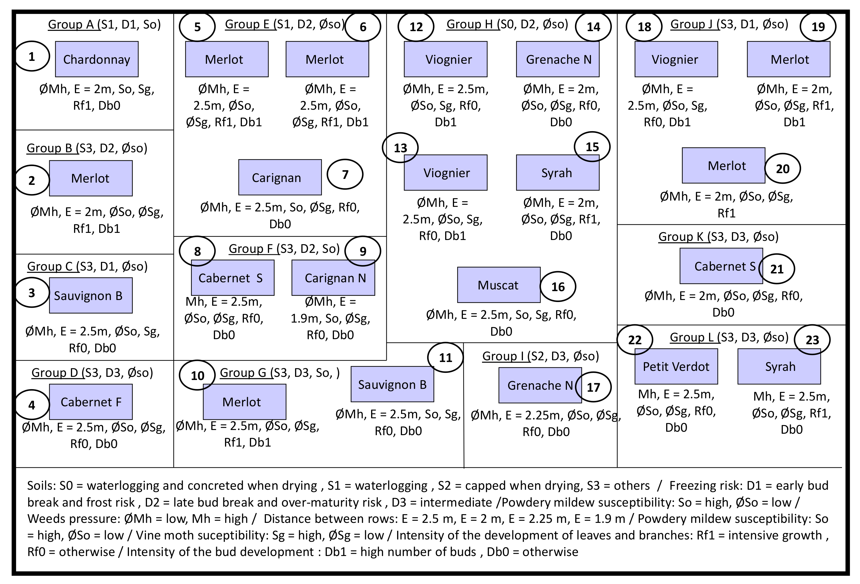
3.2. Step 2: Characterization of Specific Crop Management Sequences and Field Diversity

The objective of this step is to collect data to characterize the biophysical and technical subsystems and to describe the spatial structure of the studied farm.

Data Collection

An exhaustive inventory of the management practices between budburst and harvest was drawn up for each field: winter pruning, bud pruning, fertilization, tillage, weeding within and between the rows, pest and disease management, topping and harvest. When information on the crop management sequences for each field was unavailable, the farmer was asked if he had to make adjustments according to the characteristics of each field (e.g., whether mechanical weeding was done differently in a stony field). The farmer was also asked to explain his decisions on when and how to carry out a given management practice.

A schematic map of the vineyard was created to highlight the groups of fields and factors of heterogeneity used by the farmer for crop management. We organized the practices temporally into crop management sequences [5]. The biophysical indicators and decision-making process linking these biophysical indicators, rules and practices were also listed.

Data Analysis: Identification and Description of Groups of Fields

The vineyard studied was made up of 23 fields, arranged in 12 geographical groups of fields ranging from 0.5 ha to 6.5 ha, located around the farm at distances of 0.5 km to 5 km (Figure 2). The geographical groups of fields are lettered from A to L. Certain groups had only two fields while others were composed of five fields. They differed in terms of soil, frost risk and temperature, and powdery mildew susceptibility. No variations in wind, slope, weed pressure or wine production objectives between these geographical groups were identified. However, individual fields, numbered from 1 to 23, varied greatly in their characteristics. Seven characteristics that varied between fields were identified: weed pressure; distance between rows; powdery mildew susceptibility; vine moth pressure; leaf branch and bud development; rabbit presence and grape color. The grapevine cultivar was not considered as a whole; we preferred instead to consider certain cultivar characteristics to explain heterogeneity: bud development, leaf and branch development, and wine color.

The various management practices performed during the year were identified. These could be grouped into four types: those which affect (i) the soil and weeds (e.g., weeding, tillage, nutrient supply), (ii) pests and diseases (e.g., pesticide applications and preventative practices), (iii) the vine architecture and vegetative biomass (e.g., pruning, topping, etc.) or iv) the vine reproductive biomass (e.g., cluster thinning, harvest). Each management practice was associated with biophysical characteristics used to determine when to start a task (

Table 1. Characteristics that are taken into account to adjust the general crop management sequence for each field and their consequences on crop management at the geographical group of fields scale and at field scale.

	Selected Variables	Crop Management Operations Adjusted	Modalities Observed on the Farm	Adjustments for Each Modality
Geographical Group of Field Scale	Soil type	Tillage, and every technical operation performed with a tractor	S0 = waterlogging after rain and concreting when drying	First fields where the technical operations are performed if drying and delay if waterlogging—If drying change in the equipment
			S1 = waterlogging	Delay in the technical operations if waterlogging
			S2 = soils concreted when drying	First fields where the technical operations are performed if drying, change of the equipment
			S3 = none of these characteristics	Technical operations performed when it is not possible in the other fields
	Powdery mildew Susceptibility	Pesticide application	So = high susceptibility	Patches with a higher susceptibility first treated
			Øso = lower susceptibility	Patches treated after the others
	Root disease	Fertilization (N, P, K supply)	Mb = Root disease presence	No nitrogen supply
			ØMb = no root disease	Annual organic fertilization
	Frost risk	Pruning	D1 = early bud break and freezing risk	Last fields pruned
			D2 = late bud break with a risk of over-maturity	First fields pruned
			D3 = none of these characteristics	Intermediate
Field Scale	Selected variables	Crop management operations adjusted	Modalities observed on the farm	Adjustments for each modality
	Weeds	Mechanical weeding in the row and in the inter-row	Mh: Fields with a lot of weeds	2 mechanical weeding’s completed with a manual weeding in the row and a third intervention in the inter-row
			ØMh: Fields with not too many weeds	2 mechanical weeding’s in the row- and in the inter-row
	Width of the inter-row	Mechanical weeding, pesticides application, natural inter-cropping	Distance = 2.5m	1/4 row intercropped and 3/4 tilled-mechanical weeding with 10 teeth—Pesticide application every two rows
			Distance = 2m	1/6 row intercropped and 5/6 tilled-mechanical weeding with 7 teeth—Pesticide application every three rows
			Distance = 2.25m	1/4 row intercropped and 3/4 tilled-mechanical weeding with 10 teeth—Pesticide application every two rows
			Distance = 1.9m	1/6 row intercropped and 5/6 tilled—Manual weeding of the row—Pesticide application every three rows
	Susceptibility to powdery mildew (field)	Pesticide application	So = high susceptibility	Much longer pesticide application for high susceptibility fields, manual application if needed, application ½ rows when the distance between two rows is 2m otherwise 1/3 row
			Øso = lower susceptibility	The treatment is stopped early, no manual treatment
	Susceptibility to vine moth	Pesticide application	Sg = high susceptibility	The treatment is performed in only certain years
			Øsg = lower susceptibility	No treatment
	Leaves and branches development	Trimming	Rf1 = intensive vegetative growth	Three trimmings
			Rf0 = not intensive vegetative growth	Two trimmings
	Bud development	Bud pruning	Db1 = Intensive primary bud development	Two bud prunings
			Db0 = not intensive primary bud development	One bud pruning

). These characteristics are used by the winegrower as indicators for decision-making: for example, mechanical weeding is done when weeds reach 0.15 m high.

Three characteristics of the geographical groups of fields were taken into account by the farmer: soil type, frost risk and powdery mildew susceptibility. The links between these characteristics and their effects on management practices are presented in Table 1. Furthermore, five field characteristics identified during the interview resulted in management practices being adjusted from one field to another (Table 1). For example, the number of toppings in a field with prolific vegetative development (three toppings) differed from those in less prolific fields (two toppings). This means that potential variables of interest were identified during the interviews but they were not necessarily used by the farmer to adjust the crop management sequences to the field heterogeneity. In fact, the farmer did not take the heterogeneity related to grape color and rabbit presence into account in his management.

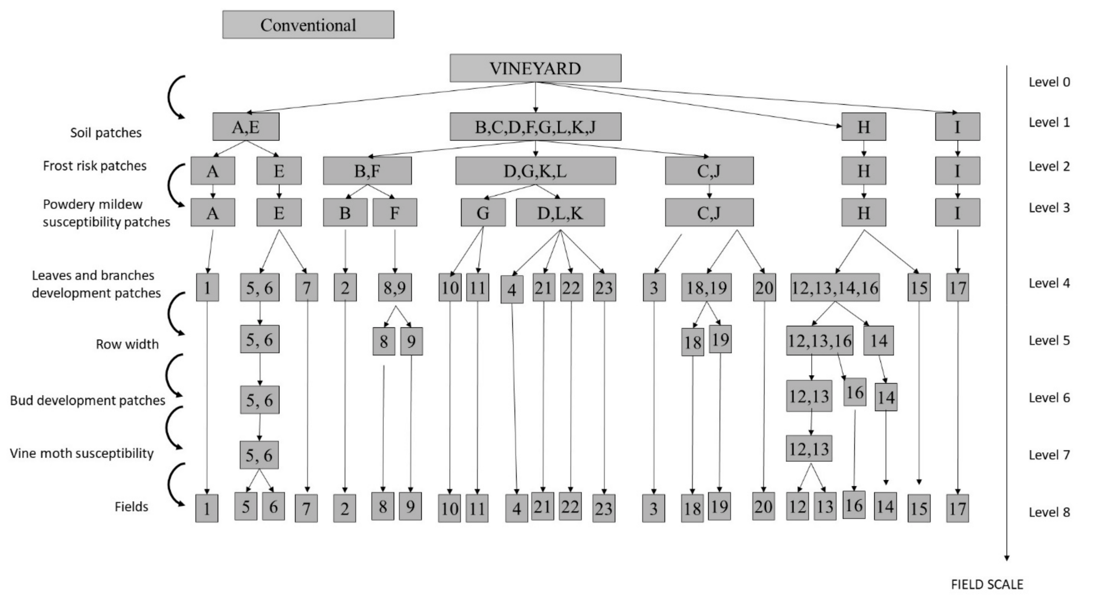
3.3. Step 3: Hierarchy of Patch Mosaics

This step consists in establishing an appropriate patch hierarchy. To do this, eight factors of heterogeneity were used to construct the farming system hierarchy: three characterizing the groups of fields and five characterizing the fields mentioned in Table 1. Two successive MCAs on the characteristics of the groups of fields and then on the individual fields helped explain the variable weight on field diversity. The vineyard was first broken down into four patches (Figure 3) by the first characteristic (e.g., according to the four soil types). Each of the four soil patches was then divided according to the three modalities of management related to frost risk. As a result, the vineyard was broken down into seven patches. They were further broken down based on the following characteristics: powdery mildew susceptibility, leaf and branch development, bud development and equal distance between rows, vine moth susceptibility and weed pressure (Figure 3). The vineyard farming system was thus divided into ten organizational and structural levels according to the order of these characteristics (

Table 2. Results of the MCA analysis-contribution of the selected variables to the first axe of MCA.

	Selected Variables	Contribution to the First Axe of MCA
Geographical Group of Fields Scale	Soil type	0.779
	Powdery mildew susceptibility	0.734
	Frost risk	0.688
Field Scale	Leaves and branches development	0.8111
	Primary bud development	0.339
	Width of the inter-row	0.429
	Vine moth susceptibility	0.109

).

These levels and the way the fields and patches of fields were spread throughout the hierarchy are presented in Table 2.

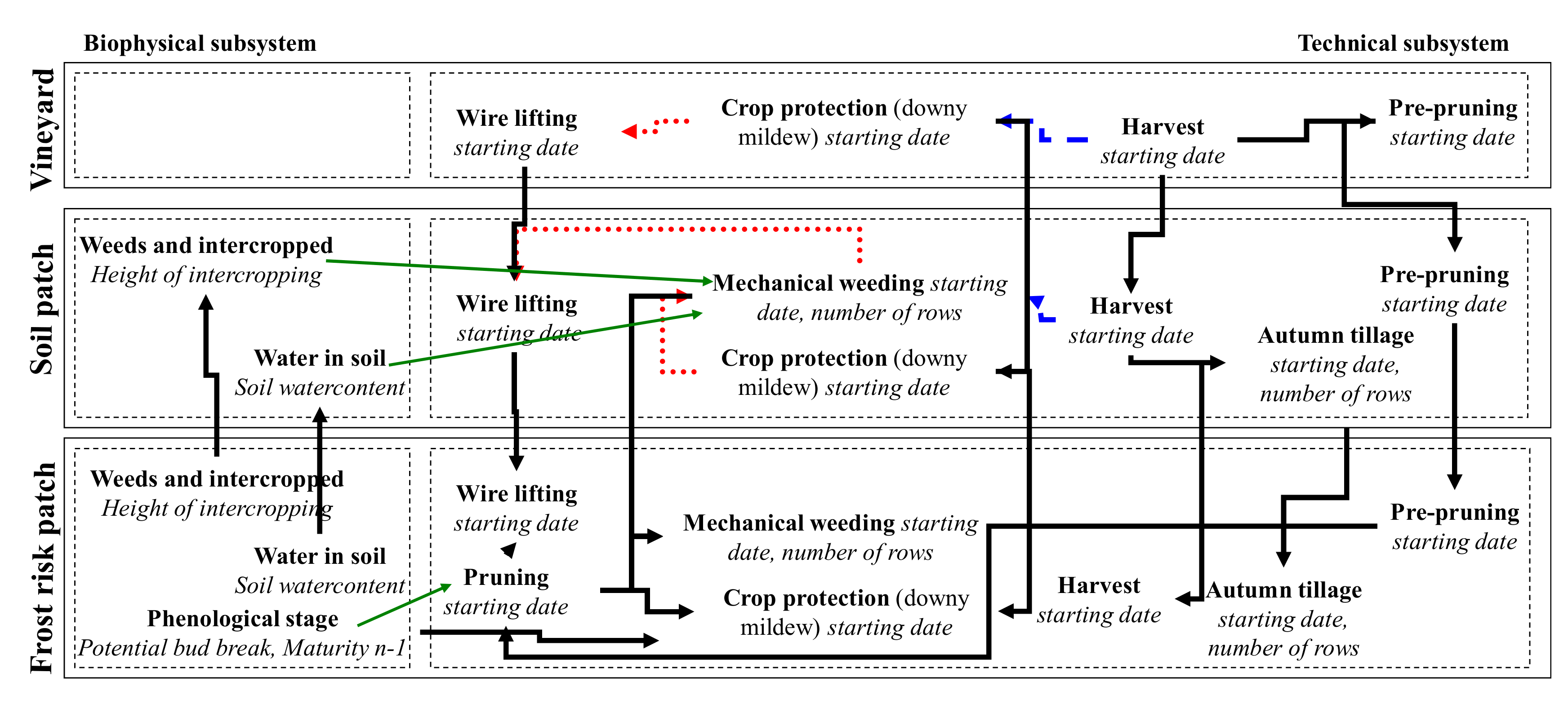
3.4. Step 4: Formalization of the Technical Subsystem

To build the technical subsystem hierarchy, the associated management practices at each level were reported along with information on decision-making processes as presented in Table 1. For example, because harvesting methods were the same for the whole vineyard, harvest is reported at vineyard level. Because the starting date for pruning was adjusted according to frost risk, pruning was positioned at the frost risk level. The management practices were then reported as extrapolations across the hierarchy in the lower levels and until the field level. For example, mechanical weeding was adjusted at soil type level

3.5. Step 5: Formalization of the Biophysical Subsystem

The various indicators used to manage management practices were positioned and linked to the management practices with which they were associated (Figure 4). These indicators have been identified in Step 2. They are part of decision rules and therefore formalize interactions between management practices and biophysical components. For example, the grapevine phenological stage was needed at the frost risk level because the phenological stage was used by the farmer to manage pruning at frost risk level. Another example, mechanical weeding was done when weeds were 0.15 m high. A biophysical component ‘weed’ was thus positioned in each patch at the level defined by the variable ‘weed’ and was characterized by the variable ‘height’.

3.6. Step 6: Spatial and Temporal Interactions between Patches and Scaling Up and Down Across Levels

All interactions between patches and across organization levels were positioned in this step. With regard to management practices, vertical interactions from higher levels to the lower levels were reported (Figure 4 for the three first levels—Figure S1). For example, if mechanical weeding at soil type level starts/stops, mechanical weeding starts/stops at frost risk level as well, with consequences at the lower levels. This means that at levels lower than soil type (levels 2 to 9), a component (here, mechanical weeding) and associated interactions were also reported.

For the biophysical subsystem, information on biophysical states of the vineyard system was up-scaled from field level to higher levels. For example, at each level from the field to frost risk levels, a phenological stage component was positioned (see Figure 4)—It aggregated information on the phenological stage of the lower levels and was aggregated at the upper level. The aggregation process from field to lower levels depends on each variable. For example, pruning was activated when one of the fields—the earliest—reached a phenological stage threshold identified in the interview. Figure 4 shows that the height of the intercropped plant was the indicator used by the farmer to determine the mechanical weeding starting date. At frost risk level, the phenological stage of the vine was used to activate pruning. The HPD representation is only qualitative at this stage but if quantitative data is needed, the aggregation method should be indicated.

Horizontal interactions between management practices at a given level of the hierarchy were also formalized in this step (Figure 4). For example, mechanical weeding was activated by pruning at frost risk level. Harvest deactivated or stopped mechanical weeding. Pre-pruning activated pruning. Information on biophysical states of the vineyard system was up-scaled from field level to higher levels.

Finally, interactions between patches are strongly related to spatial pathways of performed practices. In fact, the farmer used preferential spatial pathways to carry out management practices. For example, for pesticide application, the winegrower begins with the group of fields E, followed by groups A, B, C, D, F, G, H, J, K, L and ends with I (Figure 2). This means that regardless of the hierarchical level, when management practices had to be performed on several patches at a given level, the priority between patches was assigned according to the spatial position of patches. This was all the truer at field level. This example did not consider the ecological interactions related to pest and disease dispersion, but this could be possible for another issue.

4. Discussion

4.1. Using the HPD Conceptualization to Support Conversion towards Organic Farming

The HPD theory was successfully applied to our case study to understand and formalize the complexity of interactions within the farming system. In our case study, the farming system was broken down from the farm to the field scale, with numerous levels and associated field characteristics reflecting the complexity of farming system [2].

Considering our objective to support conversion towards organic farming, applying HPD theory made it possible to identify specific elements to take into account for conversion. Converting to organic farming implies no longer using synthetic chemicals. For vineyard systems, farmers must replace (i) herbicides in the inter-row and the row with mechanical or manual weeding, (ii) mineral fertilization with voluminous organic fertilization based on mineralization processes, (iii) chemical bud pruning with manual or mechanical bud pruning, and finally, they must stop using (iv) chemicals against powdery mildew, downy mildew and pests such as vine moths [18]. In our case study, the survey revealed that only weeding in the inter-row was already performed following organic rules. The other management practices as well as the biophysical indicators used to manage these practices must also evolve [2]. Whereas chemical weeding under the row does not require weed growth to be taken into consideration in a precise way, mechanical or manual weeding are started based on weed growth several times during the production season. Similarly, shifting from chemicals to biocontrol or sulfur/copper-based products is required to better take into account the various pest and disease susceptibilities between fields to control pest and disease risk. In the hierarchy before conversion, weed pressure under the row between fields or powdery mildew susceptibility are not used as management indicators, even when there are known differences between fields (Figure 2). This is not the case for vine moth susceptibility. Variations in bud development between fields was already taken into account, which can facilitate changes for bud pruning. Thus, the conversion to organic farming will require following at least two new biophysical indicators, weed pressure and powdery mildew susceptibility, which can result in a higher number of levels in the hierarchy. HPD representation led to planning for a more complex farming system due to the increased number of indicators for technical practice management [2].

Applying HPD theory highlighted the specific position of certain fields in the farming system. In this case study, two fields (field 1, group A and field 17, group I) differed from the others with regard to several biophysical characteristics and associated management practices. In fact, they were isolated quite high in the hierarchy (fields 1 at the third level of the hierarchy and field 17 at the second level). These fields are isolated in terms of management and consequently are time-consuming. Conversion towards organic farming in vineyard systems is a period of readjustment of the area in production with regard to available labor [18]. Farmers often decrease the area in production and vines are frequently removed in one or even two fields on the farm. In the case study, field 17 and potentially field 1 are good candidates to reduce labor requirements by decreasing the area in production. Moreover, the removal of field 17 or field 1 could limit the number of technical management sequences and the complexity of the farming system. Removing field 17 could therefore reduce the number of soil patches in the farming system from four to three.

4.2. What the HPD Framework Brings to Farming System Redesign

Applying HPD theory to the farming system redesign, which ensured more sustainability, was shown to be of significant added value because other technical system representations [3,9] do not analyze farming system organization. In several studies, the design of innovative/sustainable production systems first covers an evaluation of the performance of the current systems. This assessment often involves biophysical variables such as soil moisture content, organic matter evolution, or yield [6,7] when the assessment is at field scale. These variables are frequently of a socio-economic nature when the assessment is at the scale of the farm [8]. In both cases, the proposed alternatives in the design of new systems aiming to improve the performance of those studied often have two important limitations: (i) the variables used to select alternative activities for the newly designed innovative systems are rarely multi-criteria (including production, biophysical, socio-economic criteria) [19] or multi-scale combining variables at the level of cropping systems (yield, organic matter, etc.) and variables at farm level (gross margin, labor, farm water consumption, etc.) [8,17], and ii) the selection and feasibility of these alternatives are often limited to their agronomic and/or socio-economic performance without accounting for organizational constraints over time in line with the management of current activities [19,20]. HPD as applied here will allow us to overcome these two limits. The design of innovative systems using HPD and considering the spatial organization of the studied systems will make it possible to prioritize the systems not only according to biophysical and socio-economic criteria, but also with regard to the logic of crop management intervention (grouped in patches) in relation to the performance (e.g., yield) of these systems. On this basis, these criteria will be accounted for during the implementation of the innovative systems [20].

5. Conclusions

The adaptation of HPD theory to farming systems from ecological theory is a novel way of breaking down farming system complexity while maintaining the essential traits responsible for the overall system performance and constraints at farm level. The HPD framework requires a detailed analysis of the farming system and thorough interviews. However, it can improve the implementation of alternative farming systems that take into account the farming system complexity and the analysis of organizational changes. It is a novel way of integrating farm scale processes (e.g., organization and resources), while keeping the essence of the biophysical field diversity. In this way, it allows up- and down-scaling across farm and fields and between the socioeconomic and biophysical dimensions of the farming systems. Furthermore, the ecological background of the method will also ensure that the representation of the farming system proposed here will be compatible with the ecosystem structuration and natural resources in interaction with farming systems.

References

1. Rodriguez, D.; Cox, H.; de Voilk, P.; Power, B. A participatory whole farm modelling approach to understand impacts and increase preparedness to climate change in Australia. Agric. Syst. 2014, 126, 50–61. [Google Scholar] [CrossRef]
2. Merot, A.; Wery, J. Converting to organic viticulture increases cropping system structure and management complexity. Agron. Sustain. Dev. 2017, 37. [Google Scholar] [CrossRef] [Green Version]
3. Aubry, C.; Papy, F.; Capillon, A. Modelling decision-making processes for annual crop management. Agric. Syst. 1998, 56, 45–65. [Google Scholar] [CrossRef]
4. Schaller, N.; Lazrak, E.G.; Martin, P.; Mari, J.-F.; Aubry, C.; Benoit, M. Combining farmers’ decision rules and landscape stochastic regularities for landscape modeling. Landsc. Ecol. 2012, 27, 433–446. [Google Scholar] [CrossRef]
5. Lamanda, N.; Roux, S.; Delmotte, S.; Merot, A.; Rapidel, B.; Adam, M.; Wery, J. A protocol for the conceptualisation of an agro-ecosystem to guide data acquisition and analysis and expert knowledge integration. Eur. J. Agron. 2012, 34, 104–116. [Google Scholar] [CrossRef]
6. Merot, A.; Bergez, J.E. IRRIGATE: A dynamic integrated model combining a knowledge-based model and mechanistic biophysical models for border irrigation management. Environ. Model. Soft. 2010, 25, 421–432. [Google Scholar] [CrossRef]
7. Ripoche, A.; Rellier, J.P.; Martin-Clouaire, R.; Paré, N.; Biarnès, A.; Gary, C. Modelling adaptive management of intercropping in vineyards to satisfy agronomic and environmental performances under Mediterranean climate. Environ. Model. Soft. 2011, 26, 1467–1480. [Google Scholar] [CrossRef]
8. Hammouda, M.; Wery, J.; Darbin, T.; Belhouchette, H. Agricultural Activity concept for simulating strategic agricultural production decisions: Case study of weed resistance to herbicide treatments in South-West France. Comp. Elect. Agric. 2018, 155, 167–179. [Google Scholar] [CrossRef]
9. Belhouchette, H.; Louhichi, K.; Therond, O.; Mouratiadou, I.; Wery, J.; van Ittersum, M.K.; Lichman, G. Assessing the impact of the Nitrate Directive on farming systems using a bio-economic modelling chain. Agr. Syst. 2011, 104, 135–145. [Google Scholar] [CrossRef]
10. Wu, J.G.; David, J.L. A spatially explicit hierarchical approach to modelling complex ecological systems: Theory and applications. Ecol. Model. 2002, 153, 7–26. [Google Scholar] [CrossRef]
11. Pattee, H. Hierarchy Theory: The Challenge or Complex Systems, 1st ed.; Braziller: New York, NY, USA, 1973; 156p. [Google Scholar]
12. Meurant, G. The Ecology of Natural Disturbance and Patch Dynamics; Pickett, S.T.A., White, P.S., Eds.; Academic Press: London, UK; Orlando, FL, USA, 1985; 472p. [Google Scholar]
13. Wu, J.; Loucks, O.L. From balance to hierarchical patch dynamics: A paradigm shift in ecology. Q. Rev. Biol. 1995, 70, 439–466. [Google Scholar] [CrossRef]
14. Ratze, C.; Gillet, F.; Muller, J.P.; Stoffel, K. Simulation modelling of ecological hierarchies in constructive dynamical systems. Ecol. Complex. 2006, 4, 13–25. [Google Scholar] [CrossRef]
15. Le Gal, P.-Y.; Merot, A.; Moulin, C.H.; Navarrete, M.; Wery, J. A modelling framework to support farmer in designing innovative agricultural production systems. Environ. Model. Soft. 2010, 25, 258–268. [Google Scholar] [CrossRef]
16. Turner, M.G. Landscape Ecology: The Effect of Pattern on Process. Annu. Rev. Ecol. Syst. 1989, 20, 171–197. [Google Scholar] [CrossRef]
17. Lafond, D.; Coulon, T.; Métral, R.; Merot, A.; Wery, J. EcoViti: A systemic approach to design low pesticide vineyards. Integ. Protect. Prod. Viticulture 2013, 85, 77–86. [Google Scholar]
18. Merot, A.; Belhouchette, H.; Saj, S.; Wery, J. Implementing organic farming in vineyards. Agroecol. Sustain. Food Syst. 2019. [Google Scholar] [CrossRef]
19. Saddique, Q.; Cai, H.; Ishaque, W.; Chen, H.; Wai Chau, H.; Umer Chattha, M.; Umair Hassan, M.; Imran Khan, M.; He, J. Optimizing the Sowing Date and Irrigation Strategy to Improve Maize Yield by Using CERES (Crop Estimation through Resource and Environment Synthesis)-Maize Model. Agronomy 2019, 9, 109. [Google Scholar] [CrossRef]
20. Prost, L.; Reau, R.; Paravanoc, L.; Cerf, M.; Jeuffroy, M.-H. Designing agricultural systems from invention to implementation: The contribution of agronomy. Lessons from a case study. Agric. Syst. 2018, 164, 122–132. [Google Scholar] [CrossRef]
Figure 1. Hierarchical patch dynamics theory in farming systems derived from ecological systems [11]: framework of analysis and six-step procedure to break the farming system down into a patch hierarchy.
Agronomy 09 00604 g001
Figure 2. Farm area for the case study. The geographical groups of fields spatially separated, lettered from A to L and delimited by black lines, are characterized by three variables: soils, frost risk and powdery mildew susceptibility. Each field, numbered from 1 to 23, is characterized by the other variables. The various values taken from these variables among the fields illustrate the biophysical heterogeneity throughout the farm area. Variables in italics were not taken into account in the analysis.
Agronomy 09 00604 g002
Figure 3. Patch hierarchy established for the studied vineyard (Step 3). Each level was associated with a characteristic of the fields or geographical group of fields. (Figure 3a). The patches at a given level were created by breaking down the patches at the upper level according to the characteristics given on the left side of the figure. The letters represent the geographical groups of fields (see Figure 2) and the field numbers (see Figure 2). Each patch is composed of a technical subsystem and a biophysical subsystem.
Agronomy 09 00604 g003
Figure 4. Figure 4 shows the hierarchical breakdown of the technical and biophysical subsystems on the three first levels of organization at the end of Step 6. The interactions between the two subsystems are represented for the three first levels in the hierarchy. Each interaction could be associated with a rule linking a value or the state of the biophysical variable. Finally, Figure 4 shows also the establishment of horizontal and vertical interactions among the technical subsystem and the biophysical subsystem for the three first levels. Each arrow represents an interaction (which can be described by a decision rule) between two crop management practices: continuous thin arrow = start; thin dotted arrow = report; long dotted arrow = stop; continuous thick arrow = activate.
Agronomy 09 00604 g004