Quantitative Trait Loci (QTL) for Forage Traits in Intermediate Wheatgrass When Grown as Spaced-Plants versus Monoculture and Polyculture Swards

Abstract

It has been hypothesized that the genetic control of forage traits, especially biomass, for grass plants growing as spaced-plants versus swards is different. Likewise, the genetic control of compatibility in grass–legume polyculture mixtures is assumed to be different than for forage production in a grass monoculture. However, these hypotheses are largely unvalidated, especially at the DNA level. This study used an intermediate wheatgrass mapping population to examine the effect of three competition environments (spaced-plants, polyculture, and monoculture) on classical quantitative genetic parameters and quantitative trait loci (QTL) identification for biomass, morphology, and forage nutritive value. Moderate to high heritable variation was observed for biomass, morphological traits, and nutritive value within all three environments (H ranged from 0.50 to 0.87). Genetic correlations (r_G) among environments for morphology and nutritive value were predominantly high, however, were moderately-low (0.30 to 0.48) for biomass. Six biomass QTL were identified, including three on linkage groups (LG) 1, 6, and 15 that were only expressed in the monoculture environment. Moreover, three biomass QTL on LG 10, 14, and 15 exhibited significant QTL by environment interactions. This study verified that the genetic control of grass biomass in a monoculture versus a grass–legume mixture is only partially the same, with additional genes expressed in monoculture, and that biomass in widely spaced-plants versus swards is predominantly under different genetic control. These results indicate that selection for improved grass biomass will be most successful when conducted within the targeted monoculture or polyculture sward environment per se.

1. Introduction

Most forage breeding programs have utilized spaced-plant evaluation to select breeding materials. However, the ability of spaced-plants to predict sward biomass has been questioned [1]. Waldron et al. [2] reported a low genetic correlation of 0.37 between spaced-plant and sward biomass in tall fescue and concluded that spaced-plant evaluation would be ineffective to improve sward yield. Likewise, grass breeders have predominantly developed varieties through selection in pure (e.g., monoculture) stands. However, theory suggests that grasses bred in a monoculture environment are only exposed to intra-specific competition, and, thus, not having been exposed to inter-specific competition, will not possess the optimal biological characteristics conducive to coexistence and compatibility in grass–legume polyculture mixtures [3]. This enhanced polyculture niche differentiation has been defined as ‘ecological combining ability’ (ECA) [3]. Breeding for improved ECA is predicted to reduce competitive exclusion between plant species, whereas reciprocal recurrent breeding for ECA between grasses and legumes is predicted to improve performance of grass–legume mixtures [2,3,4]. However, this hypothesis is also largely unvalidated with only limited genetic studies attempting to investigate the role of genetics in grass–legume mixtures [4,5].

Genotype by environment interactions (G × E) affect practically every aspect of the decision-making process in plant breeding programs, including the allocation of resources in the program, choosing the testing environment, the germplasm, and breeding strategy [6]. Genotype by environment interactions in multi-environmental trials can be used to create prediction models, including determining the genotypic genetic correlations among environments for a particular trait, that can help accelerate breeding for complex traits [6,7]. A quantitative trait locus (QTL) is a chromosome region that shows statistically significant associations with one or more quantitative phenotypic traits, and QTL that are detected in multiple environments are generally considered more stable and useful for predicting across-environment performance [8]. However, QTL by environment interactions (Q × E) are useful in studying the underlying genetic correlations between different environments. The statistical analysis of Q × E is similar to that for G × E as demonstrated by Vargas et al. [9] and van Eeuwijk et al. [10]. Thus, within the QTL-mapping population, G × E interactions can be considered as being a ‘plant-based’ scale since each plant in the study is a genotype, whereas, Q × E interactions are ‘chromosome-based’ [9]. As such, G × E interactions are indicative of which parental genotypes are better adapted to specific environments within the tested environments, whereas, significant Q × E interactions are indicative of which alleles from the parental genotypes have a stronger effect in those specific environments.

Intermediate wheatgrass (IWG) [Thinopyrum intermedium (Host) Barkworth and D.R. Dewey] is a rhizomatous cool-season perennial grass with a large allohexaploid (2n = 6x = 42) genome similar to wheat [11,12] and is native to the lower mountain belts of Southern Europe, through the Middle-East and Southern Former Soviet Union to Western Pakistan [11,13]. Intermediate wheatgrass was introduced into the United States from the Maikop region of Russia in 1932 [12] and is utilized as a hay and pasture grass to increase the productivity of marginal land [11], ranking among the top species in terms of biomass potential in the Western U.S. [14,15] and other temperate regions [16,17,18,19]. Moreover, IWG is being developed as a dual-purpose perennial grain and forage crop [20,21,22,23], with major breeding efforts initiated in Canada [21] and the U.S. [11,24,25], making it the most genetically studied rangeland grass ever. Recent genetic advancements in IWG include completion of genotype-by-sequencing (GBS) to develop high-density linkage maps [12], identifying DNA markers associated with functional traits [24], and developing effective models for genomic selection [25]. Moreover, a draft genome sequence of IWG was developed, which has emerged as one of the first fully-annotated cool-season perennial grass genome sequences. These advanced genetic resources make intermediate wheatgrass a useful model for studying G × E within the complex genomes often found in forage grasses. Previous studies of the genotyped IWG population evaluated 17 traits related to seed and grain production, including stem length and maturity [26]. However, these previous studies did not evaluate biomasss or forage quality traits.

Preliminary research suggests that grass growth response is under different genetic control in non-competitive spaced-plant situations versus swards, as well as when in a grass monoculture versus a grass–legume polyculture [2,3,4]. However, there are only a few published studies that have attempted to validate these hypotheses or the grass–legume ECA concepts promoted by Hill [3], and neither hypothesis has been evaluated at the DNA level. Therefore, the objective of this study was to compare the classical quantitative genetic parameters, as well as the QTL and QTL marker by environment interactions associated with intermediate wheatgrass growth when grown in grass–grass monoculture sward (intra-specific competition), grass–legume polyculture sward (inter-specific competition), and as spaced-plants (no competition).

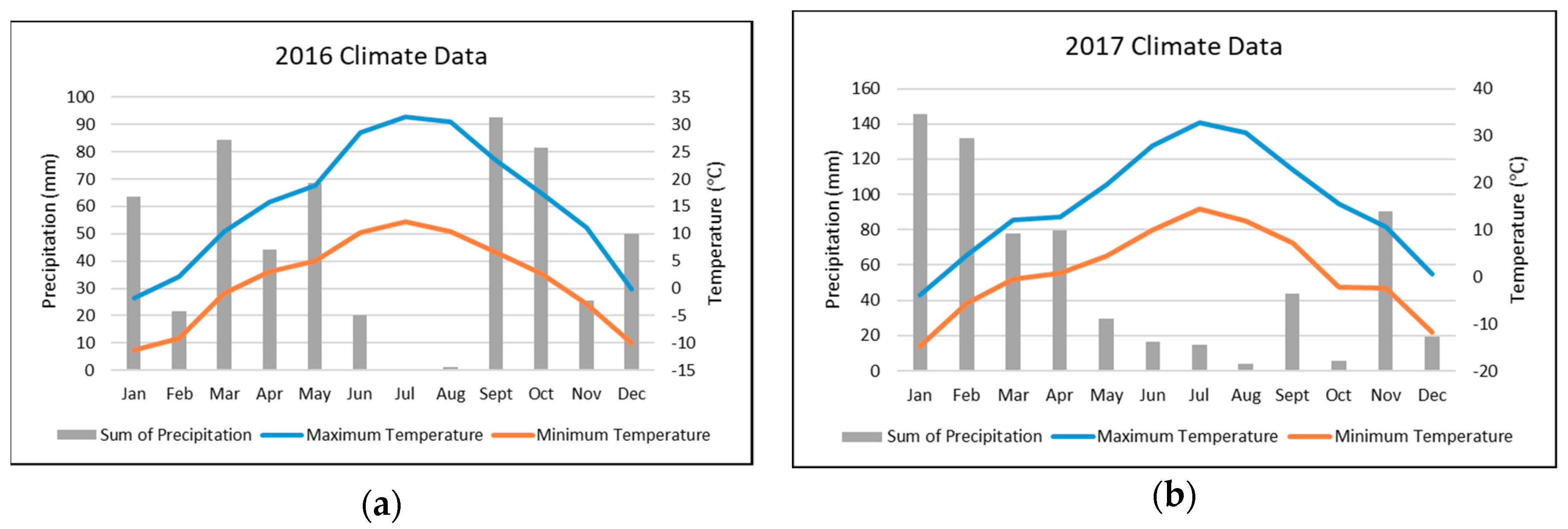
2. Materials and Methods

2.1. Plant Materials

In 2015, a subset of 192 of the 376 full-sib progeny (genets) from the M26 × M35 intermediate wheatgrass (IWG) mapping population [12,26] were established into three experimental environments, based on different systems of management and competition, using clonally replicated spaced-plant field plots. Two of the environments were established as spaced-plants in swards using the method of Van Dijk and Winkelhorst [27], by over-seeding the plots with either grasses or legumes. The plots over-seeded with grasses were considered representative of a grass monoculture sward environment with only intra-specific competition; whereas, plots over-seeded with alfalfa represented a grass–legume mixture sward environment with inter-specific competition. The third environment was a traditional spaced-plant nursery, consisting of widely spaced plants with no intra- or inter-specific competition. Plots were arranged in a split-plot randomized complete block design (RCBD) with three replications. Competition environments were considered whole-plots, whereas genets were the sub-plots. The experimental plots were established at the Utah State University Evans Research Farm, which is approximately 2 km south of Logan, UT (41°45′ N, 111°8′ W, 1350 m above sea level). The soil type at this site is a Nibley silty clay loam series (fine, mixed, active, mesic Aquic Argixeroll). Climate data at this site for the establishment and data collection years are shown in Figure 1.

The field plots were established on May 12 2015 by transplanting propagules from greenhouse started clones to the field in 2-clone plots with 0.5 m between plants and 1.1 m between rows in the monoculture and polyculture sward plots, and 1 m between rows and clones in the spaced-plants no-competition plots. The clones were split in the greenhouse during the winter by separating 18 individual tillers from each genet and then transplanting each tiller into individual cells (Ray Leach Cone-tainer SC-10 Super Cells (21 cm deep, 4 cm diameter), Stuewe and Sons, Corvallis, OR, USA) containing a 3:1 soil/peat mix where they were grown until transplanted to the field. Immediately after transplanting, the area between rows in the simulated sward plots were seeded with a drop-style fertilizer spreader following the methods of Waldron, Peel, Larson, Mott and Creech [4] with either ‘RoadCrest’ turf-type crested wheatgrass [Agropyron cristatum (L.) Gaertn.] [28] at a rate of 11.2 kg pure live seed (PLS)/ha⁻¹ (grass monoculture sward competition), or with ‘Don’ falcata-type alfalfa [Medicago sativa L. ssp. falcata (L.) Arcang.] [29] at a rate of 5.6 kg PLS/ha⁻¹ (grass–legume polyculture sward competition). This resulted in uniform, dense establishment of visibly distinct, short-statured, crested wheatgrass or alfalfa between rows. These competitive swards minimized weed competition, and, therefore, only minimal hand-weeding was required in the monoculture and polyculture swards throughout the duration of the study. The alfalfa and crested wheatgrass were mowed several times during the summer and the area between the spaced-plants no-competition rows were rototilled each fall. The field plots were irrigated weekly during the establishment year (2015), receiving 3.8 cm of water per week (approximately 100% season-long ET replacement), and thereafter did not receive supplemental irrigation. None of the three competition environments received nitrogen fertilizer.

2.2. Phenotypic Evaluations

The morphological and agronomic data (

Table 1. Trait description, abbreviation, and units of traits measured on the M26 × M35 intermediate wheatgrass mapping population evaluated over two years at Logan, UT, USA in three clonally replicated competition environments.

Trait Description	Trait Abbreviation	Units
Biomass	MASS	g plot−1
Tiller length	TILE	cm
Tillers crown−1	TICR	no.
Zadok’s maturity	ZAMA	0−99
Crude protein	CP	g kg−1 DM
Neutral detergent fiber	NDF	g kg−1 DM
Acid detergent fiber	ADF	g kg−1 DM
Acid detergent lignin	ADL	g kg−1 DM
In vitro true digestibility	IVTD	g kg−1 DM
Neutral detergent fiber digestibility	NDFD	g kg−1 NDF
Metabolizable energy	ME	Mcal kg−1 DM

) were obtained in 2016 and 2017 on a plot basis as the average of the two clones. Morphological data included growth stage, plant tiller length, and tiller number. Morphological growth stage was determined using the Zadoks scale on 20–24 June 2016 and 19–23 June 2017. In brief, the Zadoks scale is a numerical rating from 0 to 99, where 0–9 represents the germination stages, 10–19 represents the seedling growth stages, 20–29 represents the tillering growth stages, 30–39 represents the stem elongation growth stages, 40–49 represents the booting growth stages, 50–59 represents the inflorescence emergence growth stages, 60–69 represents the anthesis growth stages, 70–79 represent the milk development stages, 80–89 represents the dough development growth stages and 90–99 represents the ripening stages of development [30]. Plant tiller length and tiller number were determined when plants were predominately at the inflorescence emergence morphological stage, approaching the anthesis morphological stage, which corresponded to approximately 7 days prior to harvesting the biomass. Tiller length was measured using the average standing tiller length of the clones. The number of tillers in the monoculture and polyculture sward plots were counted by hand. However, tillers in the spaced-plants no-competition plots were too numerous to count by hand, and, therefore, the number of tillers was estimated using the following method. Briefly, the basal area of each clone was determined by measuring the diameter of actively growing tillers and using the diameter to calculate the area (i.e., basal area = π × (diameter/2)²). The number of tillers in a 5 cm cross-section of the clone were then counted, converted to tillers/cm⁻² (e.g., area of cross-section = 5 cm multiplied by diameter), and total number of tillers estimated as: total no. tillers = tillers cm⁻² × basal area.

Agronomic data consisted of biomass and forage nutritive value. Individual plots were harvested with a sickle-bar mower or hand harvested to an 8 cm stubble height on 21–22 July 2016 and from 18–20 July 2017, which corresponded to when most of the plants were at the pre-anthesis stage of plant development. Prior to each harvest, the area between rows was flailed with a mower to remove the biomass from the over-seeded plants, thus the data represents only the biomass of the IWG genets. Biomass subsamples were taken from each plot and dried to a constant weight in a forced-air oven at 60 °C and biomass on a dry-matter basis was determined. Biomass samples were ground using a Thomas Wiley Laboratory Model 4 mill (Arthur H Thomas Co, Swedesboro, NJ, USA) to pass through a 1 mm screen, and then were scanned with a Foss XDS near-infrared reflectance spectroscopy instrument (Foss, Eden Prairie, MN, USA). NIRSystem software was used to calibrate existing equations so that they were appropriate for the intermediate wheatgrass samples.

Random samples, from each environment and year, were subjected to wet laboratory analysis and used as independent calibration and validation data sets for crude protein (CP; nitrogen × 6.25), neutral detergent fiber (NDF), acid detergent fiber (ADF), acid detergent lignin (ADL), in vitro true digestibility (IVTD), Ether Extract (EE), and ash. The r-values for validation were 0.88 for ADF, 0.96 for NDF, 0.96 for CP, 0.75 for ADL, 0.90 for IVTD, 0.96 for ASH and 0.81 for EE. Samples used for wet chemistry were analyzed for N using a LECO CHN-2000 and a FP-628 Elemental Analyzer (LECO Corp., St. Joseph, MI, USA). Concentrations of NDF, ADF and IVTD, were determined following the ANKOM procedures [31,32,33,34] of the Goering and Van Soest [35]. Analyses for ADF, ADL, and NDF were made using the ANKOM-200 Fiber Analyzer (ANKOM Technology, Macedon, NY, USA). The first step of the IVTD analysis consisted of a 48 h in vitro fermentation in the ANKOM Daisy II incubator (ANKOM Technology, Macedon, NY, USA), the second step was performed with the NDF procedure mentioned above. Ash concentrations were determined by ashing at 550 °C. Ether extract analysis was done following the AOAC 2003.05 official method by a commercial lab (Dairy One, Ithaca, NY, USA). Metabolizable energy (ME) was calculated as total digestible nutrients × 0.04409 × 0.82 [36]. Total digestible nutrients (TDN) were calculated using the appropriate formula for grass:

TDN = (NFC × 0.98) + (CP × 0.87) + (FA × 0.97 × 2.25) + [NDFn × (NDFDp ÷ 100)] − 10)

(1)

where non-fibrous carbohydrates, (NFC) = 100 − (NDFn + CP +EE + ash), fatty acids (FA) = EE − 1, nitrogen free NDF (NDFn) = NDF × 0.93, NDF digestibility (NDFD) = 48 h in vitro NDF digestibility, and NDFDp = 22.7 + 0.664 × NDFD [37].

2.3. Statistical and Genetic Analysis

Morphological and agronomic data were analyzed across years using the MIXED procedure of SAS (SAS Institute Inc., Cary, NC, USA). Competition environment (e.g., spaced-plants, monoculture sward, or polyculture sward) was considered a fixed affect, whereas, year, replication, genet were considered random. Mean comparisons were made between competition environments using Fisher’s protected least significant difference (LSD) test at the p ≤ 0.05 level of probability. Pearson’s correlations among traits were estimated using SAS. Broad-sense heritabilities and standard errors were calculated within each of the three experimental environments based upon full-sibs of a perennial species evaluated at one location over multiple years using SAS REML estimates of variances as described by Holland et al. [38]. Phenotypic and genetic correlations and their standard errors were also estimated among the competition environments using SAS REML estimates as described by Holland [39].

QTL detection was performed using MapQTL version 6 model for cross-pollinator (C-P) plants using the single-QTL interval mapping (IM) procedure [40]. All the quantitative trait data were based on LSMEANS trait estimates of progeny, within and among environments, as described above. The LOD thresholds of each trait were determined using a permutation test with 1000 randomizations to control for genome-wide and chromosome-wide multiple testing with a 5% (p < 0.05) error rate. Only the most significant QTL on each linkage group was identified and compared amongst the three environments. All of the map files and locus data used for these QTL analyses were based on the integrated GBS consensus map of M26, M35, and 11 other heterozygous parents containing 21 linkage groups for both parents [12], which was constructed using a model for genetically heterogeneous cross-pollinators [41]. The MapQTL C-P map contained a total of 3856 markers, including 1699 markers that were heterozygous in the M26 parent only (with designated genotypes lm for M26 and ll for M35), 1087 markers that were heterozygous in the M35 parent only (designated genotypes nn for M26 and np for M35), and 1070 markers that were heterozygous in both parents (with designated genotype hk for both parents). In full-sib C-P families, one or more QTL may be heterozygous in one or both parents with up to four possible alleles per QTL. The C-P QTL approach fit four possible QTL alleles designated a and b corresponding to marker alleles l and m, respectively, of the first parent (M26) and QTL alleles c and d corresponding to marker alleles n and p, respectively, of the second parent (M35). This more complex C-P QTL analysis [40] has theoretical and practical advantages because three possible genotypic effects are fitted including α (difference between a and b QTL alleles), γ (difference between c and d QTL alleles) and τ (the intralocus interaction) as deviations from the overall mean (µ) value [40]. If the parents are heterozygous for the same two QTL alleles, a and b, then τ would represent a dominance deviation term. However, this was never assumed to be the case because the MapQTL C-P model always fits separate effects, α and γ, for both parents. A graphical depiction of the genetic map and relative QTL positions was developed using MapChart [42].

To analyze for significant QTL by environment interactions (Q × E), traits were analyzed by each individual statistically significant QTL marker using the MIXED procedure of SAS (SAS Institute Inc., Cary, NC, USA) and considering year (2016 and 2017), environment (Monoculture, Polyculture, and Spaced-Plants), and QTL allelic combinations as fixed effects. The marker having the highest QTL effect, measured by the Kruskal–Wallis single-point marker test [40], was employed as the independent QTL classification variable with kk, hk, or hh genotypes for biparental markers; lm or ll for M26 markers; and nn or np for M35 markers. The Kruskal–Wallis test was used because, in some cases, the IM QTL peak could have been located on a marker that had little or no effect due to the parents not being heterozygous for the same QTL alleles. Thus, the Kruskal–Wallis single-point marker test was to identify effective QTL markers, avoiding positional inferences resulting from the IM QTL mapping procedure. Mean comparisons between years, environments, or QTL allelic combination were made using Fisher’s protected least significant difference (LSD) test at the p ≤ 0.05 level of probability. To counteract the problem of many multiple comparisons, Fisher’s protected LSD mean comparisons (p ≤ 0.05) for the QTL allele by environment interactions were made only after correction to the p-value using the Bonferroni correction; where p-value was divided by the number of significant QTL markers for that corresponding trait.

3. Results

3.1. Phenotypic and Genetic Variation: Relationship Among Environments

Significant Pearson’s correlations (p < 0.05) were detected for all but one of the 55 possible pairwise comparisons among traits (

Table 2. Pearson Correlation Coefficient of the 192 full-sib progeny (genets) of the M26 × M35 intermediate wheatgrass mapping population evaluated over two years at Logan, UT, USA in three clonally replicated competition environments.

Trait	MASS	TILE	TICR	ZAMA	CP	NDF	ADF	ADL	IVTD	NDFD	ME
MASS		***	***	***	***	***	***	***	***	***	***
TILE	0.73		***	***	***	***	***	***	***	***	***
TICR	0.91	0.74		***	***	***	***	***	***	***	***
ZAMA	0.16	0.39	0.18		***	***	***	***	***	***	***
CP	−0.18	−0.21	−0.19	−0.26		***	***	—	***	***	***
NDF	0.54	0.51	0.61	0.14	−0.58		***	***	***	***	***
ADF	0.56	0.55	0.61	0.19	−0.65	0.94		***	***	***	***
ADL	0.26	0.17	0.33	−0.07	−0.01	0.25	0.32		***	*	***
IVTD	−0.60	−0.66	−0.68	−0.28	0.28	−0.64	−0.62	−0.15		***	***
NDFD	−0.26	−0.39	−0.29	−0.24	−0.18	0.10	0.08	0.04	0.70		***
ME	−0.59	−0.59	−0.66	−0.18	0.33	−0.68	−0.74	−0.37	0.87	0.49

*, **, *** Significant at the 0.05, 0.01, and 0.001 probabilities levels, respectively.

). Three relatively strong correlations (r ≥ 0.70 or r ≤ −0.70) between biomass (MASS) and tiller length (TILE), MASS and tillers crown (TICR), and TILE and TICR were observed for the biomass and morphological traits (Table 2). Whereas, there were eight relatively strong correlations (r ≥ 0.60 or r ≤ −0.60) between pairwise comparisons of forage nutritive traits (Table 2). These were comprised of primarily fiber (ADF, NDF, and IVTD) and energy (NDFD and ME) trait relationships that are well documented in the literature.

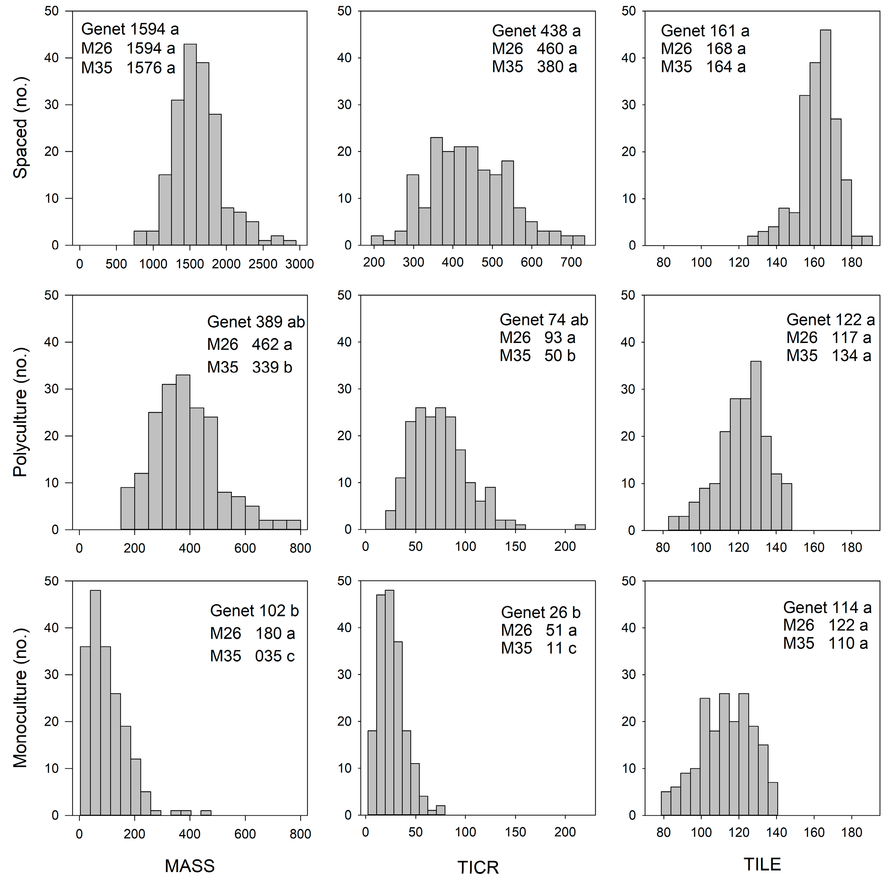
3.1.1. Biomass and Morphological Traits

Year influenced all traits, and the environment by year interaction was highly significant (p < 0.0001) for biomass and all morphological traits. This was primarily due to magnitude differences with greater MASS, and TICR in 2017 than 2016, particularly within the polyculture environment (

Table A1. Trait means ± SD by year for 192 full-sib progeny genets of the M26 × M35 intermediate wheatgrass mapping population evaluated over two years 2016–2017 at Logan, UT, USA in three clonally replicated competition environments.

Trait	Spaced-Plants		Polyculture		Monoculture
	2016	2017	2016	2017	2016	2017
MASS	1275 ± 455	1934 ± 592	123 ± 94	658 ± 304	70 ± 79	137 ± 152
TILE	164 ± 14	160 ± 17	111 ± 18	133 ± 19	116 ± 19	112 ± 20
TICR	435 ± 106	558 ± 217	30 ± 29	119 ± 68	24 ± 19	30 ± 26
ZAMA	58 ± 1	56 ± 2	55 ± 2	56 ± 3	57 ± 3	56 ± 3
CP	65 ± 13	47 ± 8	84 ± 12	63 ± 10	50 ± 11	41 ± 7
NDF	599 ± 33	654 ± 25	545 ± 33	626 ± 26	599 ± 27	595 ± 33
ADF	394 ± 19	421 ± 15	349 ± 22	399 ± 17	386 ± 16	393 ± 19
ADL	88 ± 7	95 ± 6	85 ± 9	95 ± 7	79 ± 11	93 ± 10
IVTD	694 ± 28	683 ± 22	730 ± 20	713 ± 23	726 ± 24	728 ± 31
NDFD	490 ± 33	515 ± 27	503 ± 37	541 ± 27	542 ± 38	543 ± 40
ME	2.08 ± 0.07	2.04 ± 0.07	2.21 ± 0.06	2.11 ± 0.06	2.17 ± 0.08	2.14 ± 0.07

). However, the polyculture environment also experienced greater TILE in 2017 compared to 2016, whereas, TILE did not change between years within the spaced and monoculture environments. Phenotypic data are presented as the mean across years herein.

Environments differed significantly (p < 0.05) for MASS, with the spaced-plants producing the greatest (p < 0.05) MASS, followed by the polyculture and then the monoculture environments (Figure 2). Parents M26 and M35 MASS differed significantly (p < 0.05), and mean genet MASS was intermediate within the polyculture and monoculture environments but did not differ (p > 0.05) from either parent within the spaced environment (Figure 2). Likewise, parents and mean genet TICR differed (p < 0.05) in the polyculture and monoculture environments, but not for spaced plants (Figure 2). Overall, the environments differed significantly (p < 0.05) for TILE, but average TILE for the parents and genets did not differ within environments (Figure 2). In contrast to the other morphological traits, average morphological maturity (ZAMA) did not differ (p > 0.05) among the environments, but genets were less (p < 0.05) mature than parent M35 in the Spaced and Polyculture environments (Figure 3).

Moderate to high heritable variation was observed for intermediate wheatgrass MASS and morphological traits within the three environments (H ranged from 0.50 to 0.87;

Table 3. Broad-sense heritabilities (H), and phenotypic (r_P) and genoptypic (r_G) correlations between three competition environments for 192 clonally replicated, full-sib progeny (genets) of the M26 × M35 intermediate wheatgrass mapping population evaluated over two years (2016–2017) at Logan, UT, USA.

	Spaced-Plants	Poly-Culture	Mono-Culture	Spaced-Plants vs. Polyculture		Spaced-Plants vs. Monoculture		Monoculture vs. Polyculture
Trait	H	H	H	rP	rG	rP	rG	rP	rG
MASS	0.73 ± 0.03	0.52 ± 0.07	0.61 ± 0.05	0.15 ± 0.03	0.37 ± 0.14	0.15 ± 0.03	0.30 ± 0.12	0.21 ± 0.03	0.48 ± 0.15
TILE	0.85 ± 0.02	0.84 ± 0.02	0.79 ± 0.02	0.42 ± 0.03	0.91 ± 0.04	0.32 ± 0.04	0.78 ± 0.06	0.34 ± 0.03	0.85 ± 0.05
TICR	0.53 ± 0.07	0.50 ± 0.08	0.64 ± 0.04	0.12 ± 0.03	0.59 ± 0.14	0.10 ± 0.03	0.47 ± 0.13	0.25 ± 0.03	0.62 ± 0.12
ZAMA	0.84 ± 0.02	0.87 ± 0.02	0.70 ± 0.03	0.58 ± 0.03	0.98 ± 0.02	0.50 ± 0.03	0.97 ± 0.03	0.41 ± 0.03	0.98 ± 0.04
CP	0.66 ± 0.04	0.73 ± 0.04	0.59 ± 0.07	0.23 ± 0.03	0.80 ± 0.08	0.11 ± 0.03	0.53 ± 0.12	0.16 ± 0.03	0.57 ± 0.11
NDF	0.82 ± 0.02	0.83 ± 0.03	0.69 ± 0.05	0.39 ± 0.03	0.93 ± 0.04	0.31 ± 0.04	0.92 ± 0.06	0.32 ± 0.03	0.80 ± 0.07
ADF	0.81 ± 0.02	0.81 ± 0.02	0.74 ± 0.04	0.36 ± 0.36	0.89 ± 0.05	0.32 ± 0.03	0.89 ± 0.06	0.30 ± 0.03	0.81 ± 0.07
ADL	0.62 ± 0.04	0.67 ± 0.04	0.46 ± 0.09	0.19 ± 0.03	0.94 ± 0.09	0.18 ± 0.03	1.00 ± 0.14	0.09 ± 0.03	0.66 ± 0.14
IVTD	0.81 ± 0.02	0.78 ± 0.03	0.72 ± 0.04	0.42 ± 0.03	1.01 ± 0.04	0.24 ± 0.04	0.87 ± 0.06	0.36 ± 0.03	0.90 ± 0.05
NDFD	0.79 ± 0.02	0.71 ± 0.04	0.75 ± 0.03	0.29 ± 0.03	0.94 ± 0.06	0.24 ± 0.04	0.82 ± 0.06	0.22 ± 0.03	0.65 ± 0.08
ME	0.82 ± 0.03	0.77 ± 0.03	0.78 ± 0.03	0.44 ± 0.03	0.97 ± 0.04	0.29 ± 0.04	0.84 ± 0.05	0.38 ± 0.03	0.94 ± 0.05

). The polyculture environment exhibited the lowest heritability for MASS and TICR, but the highest for ZAMA, whereas, the spaced environment had the greatest heritability for MASS, TILE, and TICR (Table 3). Phenotypic correlations between the environments for morphological traits were low to moderate, ranging from 0.10 to 0.58, however, corresponding genetic correlations were much greater, ranging from 0.47 to 0.98 (Table 3). In contrast, both low phenotypic correlations and moderately low genetic correlations between environments were observed for MASS (Table 3).

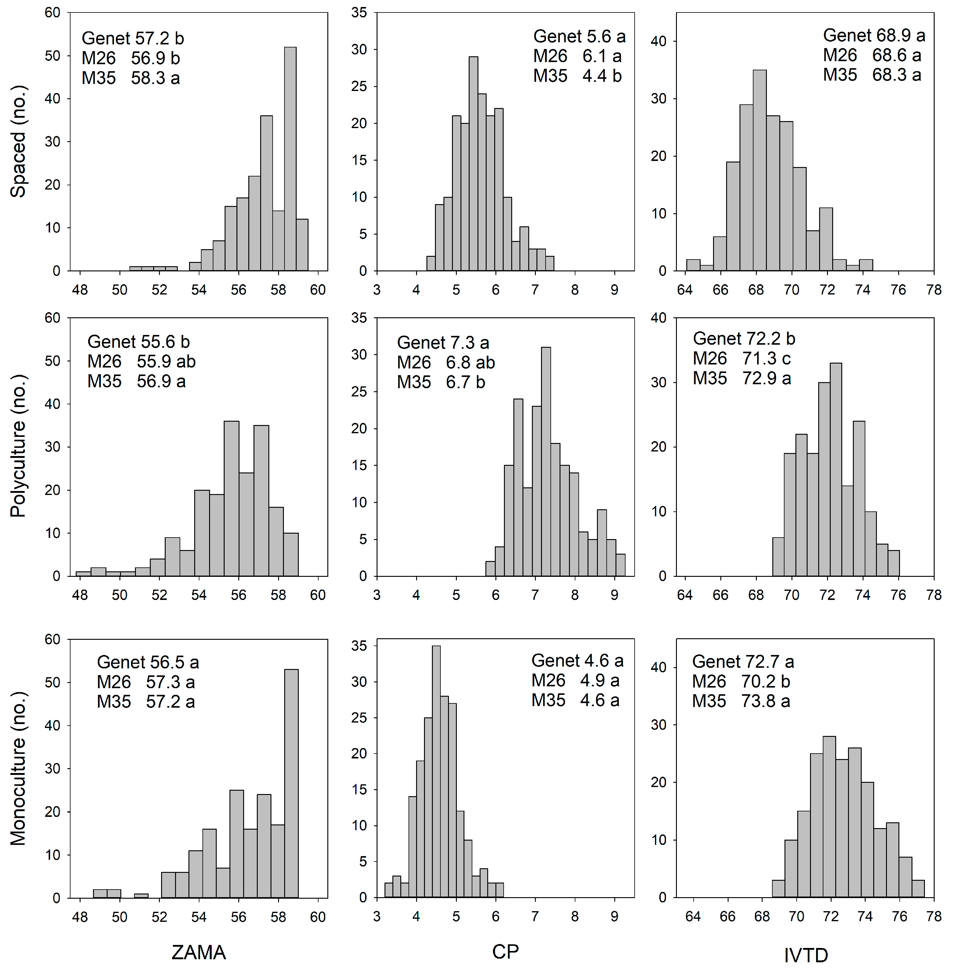
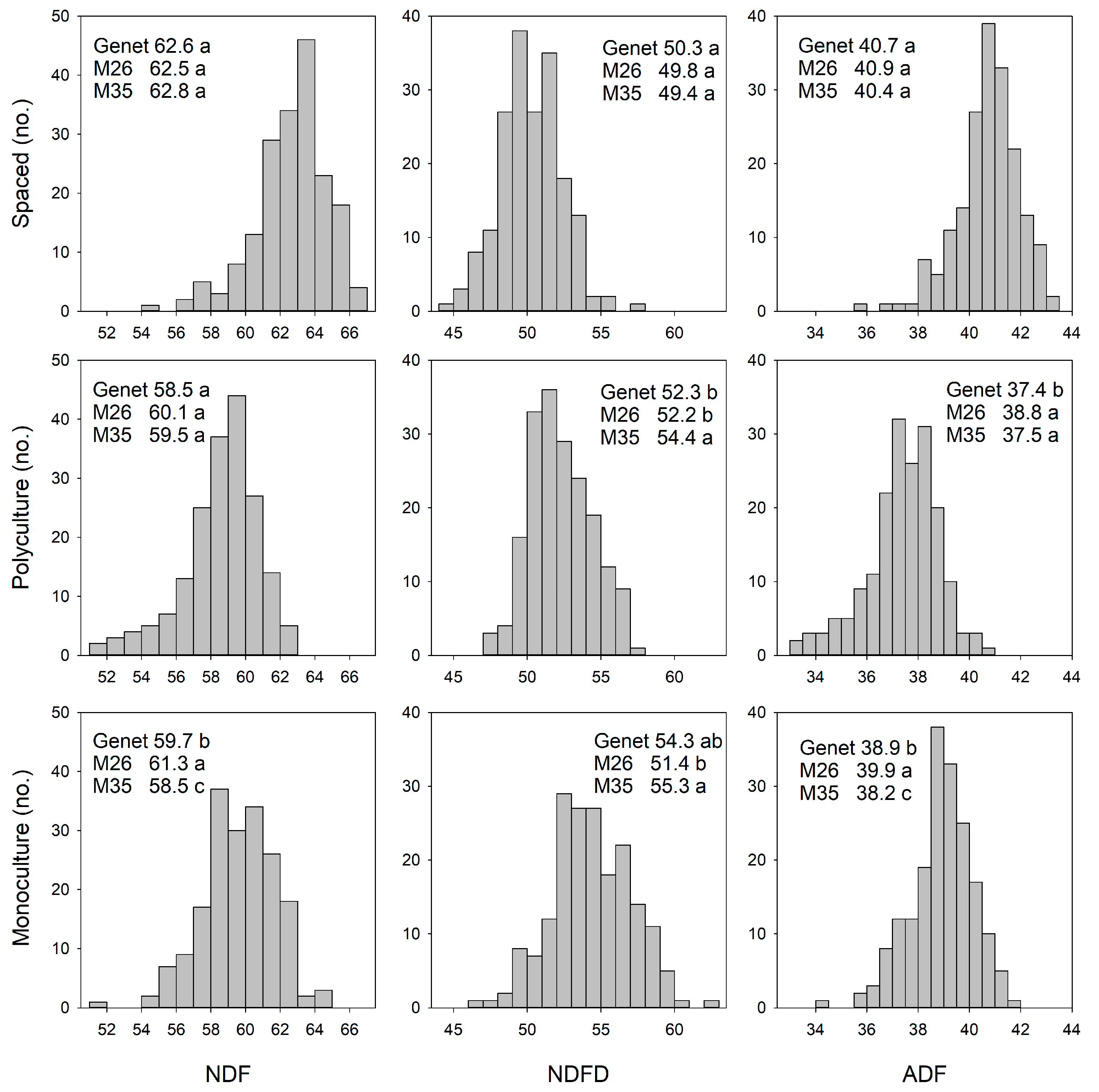
3.1.2. Forage Nutritive Value

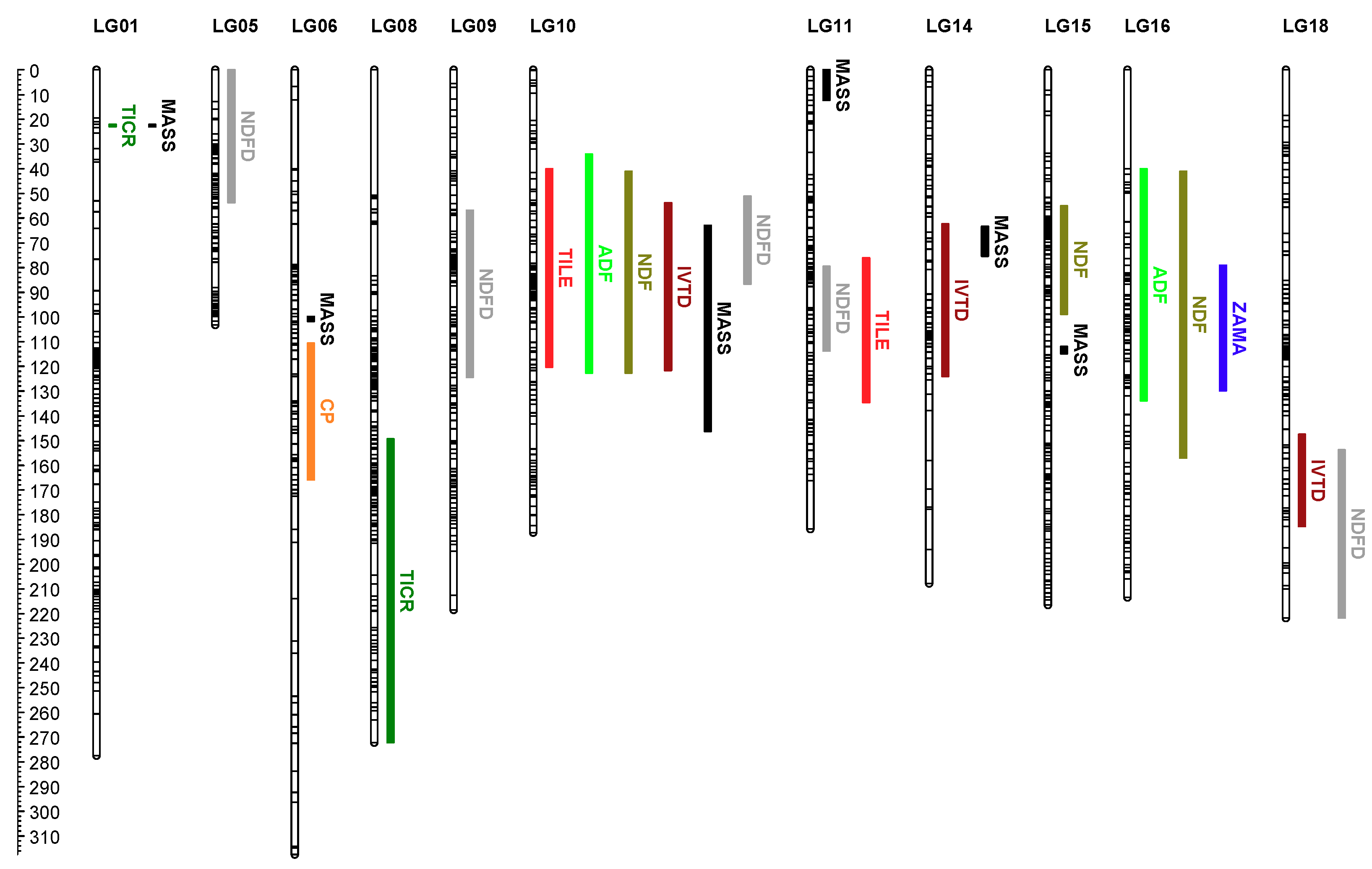
The environment by year interactions were also highly significant (p < 0.0001) for all forage nutritive traits. Again, this was primarily due to overall magnitude differences in the years, as all nutritive value traits except NDFD were more favorable in 2016 than 2017 (Table A1). However, year had the least effect within the monoculture environment, also contributing to the environment by year interaction. Forage nutritive value phenotypic data are also presented as the mean across years.

Mean forage nutritive value varied significantly (p < 0.05) amongst the three environments for all measured traits. Overall, CP, NDF, ADF, and ME were most favorable (p < 0.05) in the polyculture environment, whereas, ADL, IVTD, and NDFD were most favorable (p < 0.05) in the monoculture environment (Figure 3 and Figure 4, ME and ADL not shown). Overall, parent M35 had more favorable (p < 0.05) ADF, IVTD and ME, similar (p > 0.05) NDF and ADL, but less (p < 0.05) CP and NDFD compared to parent M26. Like biomass and morphological traits, mean genet IVTD, NDF, NDFD, and ADF did not differ (p > 0.05) from either parent in the spaced environment, but was greater (p < 0.05) than M35 for CP (Figure 3 and Figure 4). In contrast, mean genet nutritive value differed (p < 0.05) from at least one parent, and tended to be intermediate between the parents, for CP, IVTD, NDFD, and ADF in the polyculture environment, and for IVTD, NDF, NDFD, and ADF in the monoculture environment (Figure 3 and Figure 4).

With few exceptions, forage nutritive value traits were highly heritable (H > 0.70) within all three environments (Table 3). Heritable variation for ADL was moderate (H = 0.46 to 0.67), and overall, the least heritable in all three environments, relative to the other nutritive traits. Crude protein also exhibited moderate (H < 0.70) heritability in the spaced and monoculture environments (Table 3). Overall, genetic correlations between environments for forage nutritive value traits were very high, mostly exceeding r = 0.8 (Table 3). The genetic control of forage nutritive value appeared to be least similar between the monoculture and polyculture environments, with correlations of 0.57, and 0.65 for CP and NDFD, respectively. Even so, genetic correlations ranging from 0.80 to 0.94 were exhibited for the remaining nutritive traits between the monoculture and polyculture environments (Table 3).

3.2. QTL Analysis

QTL analyses were not performed on NFC or ME as they were not directly measured but calculated from the other forage nutritive values. For the C-P QTL analyses, permutation tests were conducted to determine the minimum LOD threshold required to control for 5% genome-wide error rates (p < 0.05) for each trait (

Table A2. The LOD threshold (p = 0.05) for identifying QTL within each linkage group and at the genome-wide level for 192 clonally replicated, full-sib progeny genets of the M26 × M35 intermediate wheatgrass mapping population evaluated over two years (2016–2017) in three competition environments spaced-plants, polyculture, and monoculture at Logan, UT, USA.

LG	MASS	TILE	TICR	ZAMA	CP	NDF	ADF	ADL	IVTD	NDFD
GW †	4.9	4.9	5	5.2	5	5.2	5.1	4.8	4.9	4.8
1	3.3	3.4	3.4	3.6	3.5	3.5	3.5	3.3	3.3	3.4
2	3.3	3.2	3.4	3.3	3.4	3.2	3.3	3.2	3.2	3.4
3	3.2	3.4	3.3	3.5	3.4	3.4	3.4	3.3	3.3	3.2
4	3.5	3.5	3.5	3.7	3.5	3.5	3.5	3.4	3.5	3.5
5	3.1	3.3	3.3	3.4	3.2	3.4	3.4	3.3	3.3	3.3
6	3.4	3.4	3.5	3.6	3.5	3.6	3.7	3.4	3.3	3.4
7	3.3	3.2	3.3	3.3	3.3	3.2	3.4	3.4	3.4	3.3
8	3.6	3.4	3.5	3.8	3.7	3.7	3.6	3.7	3.6	3.6
9	3.3	3.3	3.5	3.7	3.5	3.7	3.6	3.4	3.6	3.4
10	3.3	3.3	3.2	3.3	3.3	3.3	3.3	3.4	3.5	3.4
11	3.3	3.3	3.3	3.3	3.2	3.3	3.4	3.3	3.3	3.4
12	3.3	3.1	3.1	3.3	3.2	3.3	3.3	3.2	3.2	3.2
13	3.3	3.3	3.4	3.9	3.5	3.6	3.8	3.3	3.5	3.3
14	3.2	3.2	3.2	3.4	3.2	3.3	3.3	3.3	3.3	3.4
15	3.4	3.4	3.5	3.7	3.5	3.4	3.4	3.4	3.3	3.5
16	3.2	3.1	3	3.4	3.3	3.2	3.4	3.2	3.2	3.2
17	3.5	3.4	3.3	3.7	3.4	3.5	3.3	3.4	3.3	3.4
18	3.3	3.3	3.4	3.4	3.3	3.2	3.3	3.4	3.4	3.3
19	3.3	3.3	3.4	3.6	3.4	3.3	3.3	3.3	3.4	3.3
20	3.5	3.5	3.4	3.8	3.6	3.8	3.6	3.4	3.4	3.5
21	3.4	3.2	3.2	3.5	3.4	3.5	3.3	3.3	3.4	3.4

^† Genome-wide significance threshold.

). Significant linkage group-wide QTL were only reported if they were also significant on a genome-wide basis for at least one environment or the across-environment mean. Using these criteria, for all 10 traits, there were a total of 25 significant QTL detected based on three different environments or the average over all three environments (

Table 4. QTL identified for 192 clonally replicated, full-sib progeny (genets) of the M26 × M35 intermediate wheatgrass mapping population evaluated over two years (2016–2017) in three competition environments (spaced-plants, polyculture, and monoculture) at Logan, UT, USA. Only QTL with genome-wide significance in at least one environment are listed. The linkage group (LG), most significant marker LOD value, chromosomal position (cM), and percent variation explained (%R²) (only for genome-wide significance), and overall marker interval are shown.

		Spaced-Plants			Polyculture			Monoculture			Across-Environments
Trait	LG	LOD	cM	%R2	LOD	cM	%R2	LOD	cM	%R2	LOD	cM	%R2	Marker Interval
MASS	1	—			—			5.8 **	21.99	13.0	—			21.99–22.99
	6	—			—			5.1 **	99.75	11.6	—			99.75–101.75
	10	5.4 **	86.04	11.4	3.8 *	86.04		3.5 *	129.41		6.5 **	86.04	14.4	62.85–146.27
	11	—			4.0 *	7.56		5.4 **	7.56	12.3	—			0.00–12.32
	14	3.3 *	72.46		—			5.1 **	72.46	11.7	4.3 *	72.46		63.35–75.46
	15	—			—			5.9 **	111.89	13.4	—			111.89–114.89
TILE	10	5.9 **	86.04	13.6	5.5 **	69.07	12.8	4.6 *	73.7		5.7 **	86.04	13.2	40.14–120.25
	11	4.4 *	133.65		4.5 *	107.80		3.5 *	82.99		5.2 **	82.99	12.1	76.11–134.64
TICR	1	—			—			5.1 **	21.99	11..8	—			21.97–22.99
	8	5.2 **	234.70	11.8	—			—			4.7 *	234.70		149.27–272.21
ZAMA	16	6.0 **	106.27		—			—			4.2 *	107.53		79.07–129.89
CP	6	3.8 *	157.71		6.5 **	133.95	15.0	4.1 *	133.95		5.7 **	133.95	13.2	110.46–165.88
NDF	10	7.8 **	114.23	17.6	6.9 **	114.23	15.8	5.8 **	60.85	13.4	8.1 **	114.23	18.1	41.14–122.72
	15	—			—			5.7 **	69.65	13.3	—			54.96–98.79
	16	4.9 *	79.07		—			7.8 **	107.58	17.6	5.4 **	79.07	12.6	41.09–157.11
ADF	10	5.8 **	114.23	13.4	6.1 **	78.31	14.2	5.5 **	60.85	12.7	6.9 **	48.31	15.7	34.14–122.72
	16	4.8 *	70.47		—			7.6 **	109.4	17.3	5.1	79.07	11.9	40.09–133.9
IVTD	10	5.4 **	83.29	12.6	6.1 **	82.73	14.1	8.7 **	78.31	19.5	7.3 **	78.31	16.6	53.83–121.72
	14	3.8 *	108.63		3.5 *	90.65		5.2 **	68.06	12.2	5.0 **	108.63	11.6	62.35–123.98
	18	4.0 *	172.33		6.1 **	172.33	14.1	—			5.0 **	172.23	11.6	147.49–184.83
NDFD	5	4.9 **	19.73	11.6	3.8 *	0.0		—			4.1 *	0.0		0.00–53.77
	9	6.6 **	67.87	15.2	8.3 **	79.28	18.7	—			7.3 **	79.28	16.6	56.76–124.52
	10	—			—			5.3 **	66.52	12.4	—			51.08–86.72
	11	5.6 **	106.04	13.0	4.6 *	83.06		—			4.7 *	106.04		79.49–113.73
	18	3.7 *	172.33		4.9 **	177.28	11.4	3.8 *	209.97		5.3 **	177.28	12.4	153.73–221.76

*, ** Significant at the p = 0.05 level on a linkage group basis; or genome-wide basis, respectively.

, Figure 5). Of the 25 total QTL, 10 were significant within the spaced-plants environment, eight within the grass−legume polyculture environment, 14 within the grass monoculture environment, and 12 for the across-environment mean on a genome-wide basis (Table 4).

3.2.1. Biomass and Morphological Trait QTL

Six significant QTL were identified for MASS (Figure 5) of which three, on linkage groups 1, 6, and 15, were only associated with biomass in the monoculture environment (Table 4). Whereas, the other three MASS QTL, which were also significant in the monoculture environment, were exhibited in other environments; one on linkage group 11 associated with polyculture, one on linkage group 14 shared with spaced and across environments, and one on linkage group 10 significant in all environments (Table 4).

Two significant QTL were identified for TICR, one on linkage group 1 associated with the number of tillers in the monoculture environment, and one on linkage group 8 associated with the spaced environment and the across-environment mean (Table 4). Also, two QTL were identified for TILE, one each on linkage groups (LG) 10 and 11 within the spaced, monoculture, and polyculture environments (Table 4). Only one QTL was identified for ZAMA, which was associated with plant maturity in the spaced environment and across-environment mean (Table 4). These tiller length and Zadok’s maturity QTL confirm stem length (STLE) and ZAMA QTL previously reported by Larson, DeHaan, Poland, Zhang, Dorn, Kantarski, Anderson, Schmutz, Grimwood, Jenkins, Shu, Crain, Robbins and Jensen [26].

3.2.2. Forage Nutritive Value QTL

The one CP QTL, on LG 6, was associated with CP expression in all environments, although only significant on a genome-wide basis for polyculture and across-environment mean CP (Table 4). Two QTL’s were identified for the concentration of ADF in the plant, one on linkage group 10 associated with ADF in all environments, and one on 16 significant in all environments except polyculture (Table 4). Three QTL were identified for the concentration of NDF in the plant, two of which were in the same chromosomal location (LG 10 and 16) and followed the same environment-specific pattern as ADF (Table 4). The third QTL for NDF, on LG 15, was only associated with NDF expression in the monoculture environment (Table 4). No significant QTL were identified for ADL.

Three significant QTL were identified for IVTD (Table 4). Those on LGs 10 and 14 were associated with plant digestibility in all environments, whereas, the QTL on LG 18 was associated with IVTD in all environments, except monoculture (Table 4). In contrast, five QTL were associated with NDF digestibility (NDFD), but only the one on LG 18 was consistently expressed in all environments (Table 4). The NDFD QTL on LG 10 was unique to the monoculture environment, whereas, the QTL on 11, 5, and 9 were expressed in the spaced and polyculture environments, but not in monoculture (Table 4).

3.3. QTL × Environment Interactions

Three genome-wide QTL regions, comprised of seven markers, exhibited significant (Bonferroni p < 0.05) QTL by environment interaction (Q × E) (

Table 5. QTL markers exhibiting significant QTL by environment interactions (Q × E). Data from 192 clonally replicated, full-sib progeny (genets) of the M26 × M35 intermediate wheatgrass mapping population evaluated in three competition environments (Spaced-Plants, Polyculture, and Monoculture) over two years (2016–2017) at Logan, UT, USA. The lm alleles are from parent M26, the np alleles are from parent M35 and the hk alleles are from both parents.

	Trait/LG †
Marker Description	MASS/10	MASS/10	MASS/10	MASS/14	MASS/14	MASS/15	NDFD/10
Marker	TP513463	TP301824	TP799882	TP524699	TP529335	TP880985	TP301824
Position (cM)/%R2	87.08/ 18.7	73.70/ 13.1	86.04/ 23.3	65.59/ 11.4	72.46/ 11.5	61.89/ 12.4	73.70/ 21.2
Allele	hh, hk, kk	hh, hk, kk	hh, hk, kk	nn, np	nn, np	hh, hk, kk	hh, hk, kk
Env. effect
Spaced	1598.5 A	1597.6 A	1599.8 A	1609.8 A	1610.5 A	1581.9 A	50.4 C
Polyculture	383.8 B	379.1 B	381.8 B	392.4 B	390.9 B	386.2 B	52.2 B
Monoculture	99.2 C	97.6 C	99.4 C	105.0 C	104.7 C	97.9 C	54.6 A
SEM	15.2	17.4	17.6	16.5	17.1	18.8	0.17
p-value	<0.0001	<0.0001	<0.0001	<0.0001	<0.0001	<0.0001	<0.0001
Allele effect
ll, nn, or hh	752.7 A	627 C	754.2 A	735.2 A	735.7 A	640.2 B	53.3 A
lm, np, or hk	707.1 B	706.5 B	706.2 B	669.6 B	668.5 B	709.9 A	51.9 B
kk	621.8 C	740.8 A	620.7 C	N/A	N/A	715.9 A	52.0 B
SEM	15.1	17.4	17.5	15.4	15.8	18.6	0.17
p-value	<0.0001	<0.0001	<0.0001	<0.0001	<0.0001	0.0006	<0.0001
Env. × Allele effect
Spaced × ll, nn, or hh	1739.2 A	1481.3 C	1744.6 A	1674.7 A	1686.9 A	1461.9 B	51.2 F
Spaced × lm, np, or hk	1604.6 B	1610.2 B	1597.0 B	1544.9 B	1534.1 B	1617.8 A	49.9 G
Spaced × kk	1451.6 C	1701.3 A	1458.0 C	N/A	N/A	1666.1 A	49.9 G
Poly × ll, nn, or hh	407.5 D	330.1 E	408.1 D	414.4 C	407.4 C	368.7 C	52.6 D
Poly × lm, np, or hk	406.7 D	399.2 D	409.3 D	370.4 D	374.5 C	399.8 C	52.1 E
Poly × kk	337.4 E	408 D	328.1 E	N/A	N/A	390.1 C	51.9 E
Mono × ll, nn, or hh	111.3 F	69.7 F	109.9 F	116.4 E	112.7 D	90.1 D	55.9 A
Mono × lm, np, or hk	110 F	110.1 F	112.4 F	93.6 E	96.8 D	112.2 D	53.7 C
Mono × kk	76.3 F	113.1 F	75.9 F	N/A	N/A	91.4 D	54.2 B
SEM	18.8	23.6	24.1	19.4	20.6	26.4	0.22
p-value	<0.0001	0.0008	<0.0001	0.0004	<0.0001	0.0007	0.0003
Bonferroni p-value	0.0031	0.0031	0.0031	0.0031	0.0031	0.0031	0.0026

^† Values within a column followed by a different letter (A,B,C) indicate that the environment, allele, or environment × allele means are significantly different than each other at the 0.05 level of probability.

). However, of these seven markers, six were associated with MASS, while the remaining marker was associated with a Q × E effect on a NDFD (Table 5). The three MASS QTL markers on LG 10 were comprised of alleles from both parents (i.e., h and k), and the different allelic combinations of hh, hk, and kk were associated with significant differences (p < 0.05) in MASS in the spaced-plants and polyculture environments but had no effect on MASS in the monoculture environment (Table 5 and

Table A3. Significance of QTL by environment interactions (Q × E), and estimates of QTL effects (α, γ) as a percentage of population mean where α is difference between QTL alleles of the M26 parent and γ is difference between QTL alleles of the M35 parent. QTL were identified for 192 clonally replicated, full-sib progeny (genets) of the M26 × M35 intermediate wheatgrass mapping population evaluated over two years (2016–2017) in three competition environments (spaced-plants, polyculture, and monoculture) at Logan, UT, USA. Only QTL with genome-wide significance in at least one environment are listed.

Trait	Linkage Group	Spaced−Plants	Polyculture	Monoculture	Across Environments	Q × E
MASS	1	(0.01, −0.30)	(0.00, 0.02)	(0.01, −0.33) **	(0.01, −0.30)	NS
	6	(−0.03, 0.00)	(−0.01, 0.01)	(−0.13, 0.12) **	(−0.08, 0.09)	NS
	10	(−0.08, 0.09) **	(−0.02, 0.02) *	(0.01, 0.01) *	(−0.04, 0.04) **	0.0001
	11	(−0.01, −0.02)	(0.00, −0.02) *	(0.00, −0.01) **	(0.00, −0.01)	NS
	14	(−0.01, −0.08) *	(0.01, −0.02)	(0.00, −0.01) **	(0.00, −0.03) *	0.0004
	15	(−0.11, 0.02)	(−0.01, −0.01)	(−0.13, 0.11) **	(−0.08, 0.04)	0.0007
TILE	10	(−3.13, 2.15) **	(−3.92, 2.72) **	(−3.69, 2.8) *	(−3.24, 2.34) **	NS
	11	(2.32, 0.54) *	(2.84, −1.97) *	(2.78, −2.74) *	(2.61, −2.28) **	NS
TICR	1	(31.42, −56.82)	(0.58, −32.17)	(1.09, −79.75) **	(12.03, −199.51)	NS
	8	(34.5, 29.51) **	(2.66, 11.88)	(0.40, 5.66)	(10.43, 6.09) *	NS
ZAMA	16	(−0.40, 0.38) **	(2.73, −5.06)	(−0.29, −1.19)	(−0.43, 0.29) *	NS
CP	6	(0.13, −0.12) *	(0.18, 0.15) **	(0.08, 0.08) *	(0.13, 0.07) **	NS
NDF	10	(−0.42, 0.53) **	(−0.36, 0.64) **	(−0.30, 0.73) **	(−0.35, 0.57) **	NS
	15	(−0.08, 0.43)	(−0.09, 0.24)	(−0.04, 0.81) **	(−0.05, 0.51)	NS
	16	(0.44, −0.62) *	(0.18, −0.48)	(0.44, −0.73) **	(0.38, −0.61) **	NS
ADF	10	(−0.21, 0.27) **	(−0.24, 0.44) **	(−0.14, 0.43) **	(−0.05, 0.45) **	NS
	16	(0.24, −0.32) *	(0.10, −0.3)	(0.26, −0.43) **	(0.23, −0.36) **	NS
	10	(0.30, −0.51) **	(0.39, −0.41) **	(0.59, −0.76) **	(0.33, −0.48) **	NS
	14	(−0.24, 0.46) *	(−0.14, 0.4) *	(−0.08, 0.56) **	(−0.23, 0.48) **	NS
	18	(0.18, 0.53) *	(0.36, 0.49) **	(0.24, 0.56)	(0.25, 0.48) **	NS
NDFD	5	(0.19, 0.19) **	(0.14, 0.48) *	(0.08, 0.33)	(0.21, 0.4) *	NS
	9	(−0.17, −0.78) **	(0.27, −0.85) **	(0.16, −0.64)	(0.22, −0.74) **	NS
	10	(0.25, −0.35)	(0.29, −0.09)	(0.47, −0.49) **	(0.32, −0.27)	0.0003
	11	(−0.40, −0.34) **	(−0.47, −0.39) *	(−0.41, 0.03)	(−0.40, −0.25) *	NS
	18	(0.37, 0.51) *	(0.50, 0.49) **	(0.41, 0.49) *	(0.40, 0.51) **	NS

*, ** Identified QTL significant at the p = 0.05 level on a linkage group basis; or genome−wide basis, respectively. NS indicates that Q × E was not significant at the p ≤ 0.05 level.

). In contrast, the two MASS QTL markers on LG 14 were comprised of alleles from the M35 parent (i.e., n and p). These nn and np allelic combinations also had no effect on MASS in the monoculture environment, but the alleles for marker TP524699 were associated (p < 0.05) with MASS differences in the spaced-plants and polyculture environments, whereas, TP529335 alleles were only associated with MASS differences (p < 0.05) in the spaced-plants environment (Table 5 and Table A3). In comparison, the MASS QTL on LG 15 was comprised of alleles from both parents and had an overall large effect on MASS in the monoculture environment (Table A3), but the significant Q × E effect was due to allelic combinations associated with MASS differences (p < 0.05) only in the spaced-plants environment (Table 5). The significant Q × E for forage nutritive value was for NDFD marker TP301824 on LG 10 and comprised of alleles from both parents (i.e., h and k) (Table 5). The homozygous hh alleles for T301824 resulted in more favorable NDFD in all three environments, but the homozygous kk allelic state was associated with greater NDFD, as compared to heterozygous hk, only in the monoculture environment (Table 5).

4. Discussion

4.1. Genetic Control in Spaced-Plants and Swards

4.1.1. Spaced-Plant vs. Sward: Biomass and Morphological Traits

Both Waldron, Robins, Peel and Jensen [2] and Hayward and Vivero [43] surmised that biomass in spaced and sward environments might be under different genetic control. However, prior to this study, this hypothesis had not been evaluated at the DNA level. Similar to Waldron, Robins, Peel and Jensen [2], we found low genetic correlations of 0.37 and 0.30 for MASS between intermediate wheatgrass spaced-plants and simulated polyculture and monoculture swards, respectively, further suggesting genetic control of biomass is dependent upon the level of inter-plant competition in the environment. Six different QTL affected MASS production (Table 4). This is the first known report of genetic mapping of biomass in intermediate wheatgrass, but is similar to the Larson et al. [44] report of eight biomass QTL in interspecific hybrids between Basin and Creeping wildryes [Leymus cinereus Scribn. and Merr. Á. Löve] and [Leymus triticoides Buckley Pilg.]. Our hypothesis that biomass genetic control is dependent upon the environment was supported by the varying number of QTL identified for each environment, two for each of the spaced-plant and polyculture environments, and six within the monoculture environment (Table 4). It is noteworthy that both spaced-plant QTL on LGs 10 and 14 were also significant in the monoculture environment, as well as the QTL on LG 10 also being significant in the polyculture environment, suggesting the presence of major biomass coding regions at these chromosomal locations.

Six MASS QTL markers exhibited a significant allele by environment interaction, of which five were markers for the shared MASS QTL on LGs 10 and 14 (Table 5). However, within these five markers, no allelic rank changes were exhibited for MASS between environments, rather, the Q × E interactions resulted from magnitude differences among environments and the inability to detect allelic differences in the polyculture and monoculture sward environments (Table 5). Therefore, this is further evidence that the QTL on these LGs (LG 10 and 14, Figure 5) contain major MASS coding regions regardless of environment and supports the presence of at least some genetic correlation between spaced-plant and sward environments. It is also likely that those QTL contain the predominant coding regions for spaced-plant MASS, as evidenced by significant differences in MASS associated with the allelic combinations predominantly in the spaced-plant environment (Table 5). Whereas, the MASS QTL identified on LGs 1, 6, and 15 within the monoculture environment, and a QTL on LG 11 identified in both monoculture and polyculture (Table 4), likely contain additional coding regions that largely contribute to MASS when in a more competitive environment as opposed to the non-competitive environment of spaced-plants. Overall, these data validate the low genetic correlations reported herein and by Waldron, Robins, Peel and Jensen [2], and provide evidence that biomass in spaced-plants and swards is mostly under different genetic control.

Spaced-plant and sward TILE were genetically correlated (r_G = 0.91 and 0.78 for the polyculture and monoculture, respectively), and very similar to the genetic correlation of 0.85 between height of tall fescue spaced-plants and swards reported by Waldron, Robins, Peel and Jensen [2]. Two QTL were identified for TILE (Table 4). Tiller length was highly correlated with biomass (Pearson’s r = 0.73, Table 2); therefore, it was not surprising that a TILE QTL shared across all environments identified on LG 10 corresponded to the same location as one of the two major shared MASS QTL (Table 4, Figure 5). A TILE QTL common across all environments was also identified on LG 11, but it was not at the same chromosome interval as the MASS QTL on LG 11 (Table 4, Figure 5). In comparison, Larson, DeHaan, Poland, Zhang, Dorn, Kantarski, Anderson, Schmutz, Grimwood, Jenkins, Shu, Crain, Robbins and Jensen [26] identified eight tiller length QTL using this same intermediate mapping population, of which only the QTL on LG 11 was the same between the two studies. Interestingly in the Larson, DeHaan, Poland, Zhang, Dorn, Kantarski, Anderson, Schmutz, Grimwood, Jenkins, Shu, Crain, Robbins and Jensen [26] study, this LG 11 QTL was significant at the same Utah location as our study, but not at their Kansas site, suggesting that this QTL contains genes coding for TILE when in more arid environments. The high genetic correlation, 100% shared QTL amongst environments, and lack of QTL markers with significant Q × E interaction suggest that TILE is under similar genetic control whether in a spaced-plant or sward environment.

Tillers crown⁻¹ was highly correlated with biomass (r = 0.91), and as such, TICR in spaced-plant and both sward environments were only moderately genetically correlated (r_G = 0.59 and 0.47, for polyculture and monoculture, respectively). Waldron, Robins, Peel and Jensen [2] reported slightly higher genetic correlation (r_G = 0.67) between spaced-plants and swards for tiller density in tall fescue but given the different growth habit of these two species (rhizomatous versus non-rhizomatous for IWG and tall fescue, respectively), such slight differences in tiller density and number would be expected. Two QTL were identified for TICR as compared to four previously identified in this population [26]; however, both studies identified a TICR QTL on LG 8. Larson, DeHaan, Poland, Zhang, Dorn, Kantarski, Anderson, Schmutz, Grimwood, Jenkins, Shu, Crain, Robbins and Jensen [26] used spaced-plant evaluation, and likewise, the LG 8 QTL was only significant for our spaced-plant environment (Table 4), further validating the importance of this QTL for TICR in non-competitive environments. However, we also identified a TICR QTL on LG 1 that was only significant in the monoculture sward, which corresponds to the same interval location as our monoculture-only LG 1 MASS QTL (Table 4, Figure 5). Thus, there is QTL evidence for the low to moderate genetic correlation between spaced-plants and swards for TICR. Overall, morphological traits were found to be partially under the same genetic control between spaced-plant and sward environments; however, genetic control of those traits that were most correlated with biomass, such as TICR, were more affected by the specific environment.

4.1.2. Spaced-Plant vs. Sward: Forage Nutritive Value

Waldron, Robins, Peel and Jensen [2] reported that spaced-plant evaluation was moderately predictive of sward nutritive fiber and digestibility but not predictive of CP in tall fescue. In comparison, our forage nutritive trait genetic correlations between spaced-plant and sward environments were even higher than that reported by Waldron, Robins, Peel and Jensen [2]. Furthermore, we also found that the spaced-plant environment was only moderately predictive of CP in a grass monoculture (Table 3). Since we did not apply supplemental fertilizer, this discrepancy in CP between the non-competitive spaced-plant and highly competitive monoculture environments were probably mostly due to N availability. This hypothesis is based upon the assumption of some N-transfer between the alfalfa to the grass in the polyculture environment [45,46], and is consistent with a much greater r_G of 0.80 between spaced-plant and polyculture as compared to 0.53 between the spaced-plant and monoculture environments (Table 3). However, QTL data did not fully support this conclusion since we only identified one CP QTL on LG 6 that was shared by both the spaced-plants and the monoculture and polyculture sward environments (Table 4).

Fiber digestibility (NDF and ADF) were highly genetically correlated (r_G ≥ 0.89) between spaced-plant and sward environments, and greater than that reported by Waldron, Robins, Peel and Jensen [2] of 0.56 and 0.70, for NDF and ADF, respectively. However, our QTL data are more in agreement with their study, since only one of three identified NDF QTL was shared amongst the spaced-plant and monoculture and polyculture sward environments (Table 4). It is noteworthy that the two identified ADF QTL on LGs 10 and 16 were in the same chromosomal interval as two of the NDF QTL (Figure 5), providing genetic validation of the relationship between these two highly correlated (e.g., r = 0.94 in this study) fiber traits. In contrast, based upon our high genetic correlations 0.87 to 1.00 and two of three IVTD QTL shared amongst environments, this study completely supports Waldron, Robins, Peel and Jensen’s [2] assumption that whole grass plant digestibility is under similar genetic control in both spaced-plants and swards. In addition, we identified a QTL on LG 10 that is significant for both MASS and IVTD and shared by all environments (Table 4, Figure 5), suggesting that gene(s) in this chromosomal region may be primarily responsible for the negative correlation between biomass and digestibility in grasses (r = −0.64 in this study).

4.2. Genetic Control in Grass Monoculture and Grass−Legume Polyculture

4.2.1. Monoculture vs. Polyculture: Biomass and Morphological Traits

Historically, grass breeders have developed varieties through selection in pure (e.g., monoculture) stands. However, the benefits of a grass−legume mixture may be enhanced if the grass and the legume have greater ecological combining ability [3]. This is based upon the theory that monoculture and polyculture environments are different due to intra-specific versus inter-specific competition and as such, plant growth is under unique genetic control within each environment. This hypothesis is largely unvalidated with only limited genetic studies attempting to investigate the role of genetics in grass−legume mixtures [4,5]. Accordingly, this study presents both classical and DNA-based quantitative genetic analysis to evaluate the genetic control of grasses growing in monoculture versus grass−legume polyculture.

We found an intermediate level of genetic correlation (r_G = 0.48) for biomass between grass monoculture and grass−legume polyculture environments (Table 3). In comparison, Waldron, Peel, Larson, Mott and Creech [4] reported r_G ranging from −0.31 to 0.92, depending upon harvest, between tall fescue biomass in monoculture versus polyculture environments. However, given that we used 1-harvest management strategy, their first harvest results are most comparable to our results. As such, their first harvest biomass, the greatest of the four cuttings comprising 36% of annual biomass, exhibited the exact same genetic correlation (r_G = 0.48) between the monoculture and polyculture environments [4] as reported herein. Furthermore, in both studies, heritability was consistently greater in the monoculture compared to the polyculture environment.

Six QTL were identified associated with biomass in monoculture, whereas, only two were associated with biomass in polyculture (Table 4). However, it is important to note that both of these QTL were shared by the two environments and included the major QTL on LG 10 that was also associated with spaced-plants. Three biomass QTL markers on LG 10 exhibited significant Q × E interaction as a result of specific alleles being associated with biomass differences in polyculture as well as spaced-plants, but not significantly different in the monoculture (Table 5). Thus, these data support the existence of a major biomass QTL on LG 10, that is predominant for biomass production in polyculture and non-competitive spaced-plants but less so for the highly competitive monoculture environment. The additional biomass QTL on LGs 1, 6, 14, and 15 identified in the monoculture environment, further indicate that biomass in monoculture is under more complex genetic control, possibly due to the increased intra-plant competition for water and nitrogen. Similar patterns of this more complex genetic control in monoculture compared to polyculture were evident for morphological traits. For instance, although no QTL were identified for TICR in the polyculture environment, a LG 1 TICR QTL was identified in the monoculture environment corresponding to a monoculture-specific biomass QTL at the same chromosomal position (Table 4, Figure 5).

Overall, these data indicate that genetic control of biomass and morphology of grass grown in a monoculture versus a grass−legume mixture are partially different, with more complex genetic control within the monoculture as additional genes are expressed possibly due to increased intra-plant competition. Given that we did not apply supplemental N or irrigation during this study, there are possible underlying physiological N-capture and drought-response explanations for these findings. Different rooting depth of intermediate wheatgrass and alfalfa would result in less competition for soil moisture in the polyculture environment compared to monoculture. It is also probable that there was more N available to the grass in the polyculture due to the legume transfer of atmospheric fixed nitrogen [45,46]. This hypothesis is supported by greater biomass and CP in the polyculture compared to the monoculture (Figure 2 and Figure 3). Some grass genotypes may also be more efficient in capturing and utilizing this atmospheric-fixed nitrogen and/or are more compatible with the soil biota associated with nitrogen-fixing legumes. Zuppinger-Dingley et al. [47] reported that in several grass species, the grass plants had a changed metabolic fingerprint when grown in grass−legume mixtures versus grass monocultures. They hypothesized that the biochemical composition differences may have been due to rapid co-evolution of the plants with the soil biota, with the primary selection factor being negative plant–soil feedback in the monocultures. This negative feedback may result in differential gene expression between polyculture and monoculture, as evidenced by the QTL results herein.

4.2.2. Monoculture vs. Polyculture: Forage Nutritive Value

Intermediate wheatgrass plants in the polyculture environment had more favorable CP, NDF and ADF (measure of cellulose and hemicellulose, respectively), but less favorable IVTD and NDFD (measure of whole plant digestion) compared to the monoculture environment (Figure 3 and Figure 4). This is mostly in agreement with other studies that also reported that forage nutritive value of grasses improves when grown in grass–legume mixtures [48,49]. Genetic correlations ranged from 0.57 for CP to 0.90 for IVTD between the polyculture and monoculture environments, suggesting mostly similar genetic control (Table 3). However, only 6 of 14 forage nutritive value QTL were in common between the two environments (Table 4). Interestingly, the environment in which a nutritive trait had a more favorable value also had less QTL identified for those traits, except for the CP (Table 4), suggesting that more complex genetic control is associated with decreased nutritive value. A significant Q × E interaction for NDFD, with allelic rank changes for NDFD between the monoculture and polyculture swards, provides some evidence that nutritive value is at least partially under different genetic control in monoculture and polyculture environments (Table 5). Thus overall, our QTL data only partially corroborate the moderate to high classical genetic correlations we found for forage nutritive value between monoculture and polyculture. We are not aware of other genetic studies comparing forage nutritive value of a grass growing in monoculture versus grass–legume polyculture. Thus, we conclude that forage nutritive value is probably partially to mostly under the same genetic control in monoculture and polyculture environments.

5. Conclusions

The M26 × M35 intermediate wheatgrass mapping population was evaluated over two years in three competition environments (spaced-plants, polyculture, and monoculture) to determine the effect of these environments on classical quantitative genetic parameters and on QTL identification for biomass, morphology, and forage nutritive value. Moderate to high heritable variation was observed for intermediate wheatgrass biomass and morphological traits within the three environments (H ranged from 0.50 to 0.87), and with few exceptions, the forage nutritive value traits were highly heritable (H > 0.70) within all three environments. However, in contrast to the high values among environment genetic correlations for plant morphology and nutritive value, the genetic correlations between environments for biomass were moderately low (r_G of 0.30 to 0.48). A total of 25 significant QTL were identified, of which 10 were significant within the spaced-plants environment, 14 within the grass monoculture environment, and eight within the grass–legume polyculture environment. Six QTL were identified for biomass, including QTL on LGs 1, 6, and 15, that were only expressed in the monoculture environment. However, data suggested the presence of a major biomass QTL on LG 10 in polyculture swards and non-competitive spaced-plants, but with much less effect in the highly competitive monoculture environment. Moreover, six QTL biomass markers exhibited a QTL allele by environment interaction, with those on LGs 1, 6, 11, and 15 appearing to contain regions largely contributing to biomass in swards as opposed to the non-competitive environment of spaced-plants. These QTL data validated the previously reported low genetic correlations for biomass between spaced plants and swards, providing DNA evidence that biomass in spaced-plants and swards is predominantly under different genetic control. Furthermore, results indicated that the genetic control of grass biomass in a monoculture versus a grass–legume mixture are partially different, with more complex genetic control within the monoculture as additional genes are expressed, possibly due to increased intra-plant competition. Overall, we conclude that breeding and selection for improved grass biomass within the targeted monoculture or polyculture sward environment per se is warranted.

References

1. Casler, M.D.; Carlson, I.T.; Berg, C.C.; Sleper, D.A.; Barker, R.E. Convergent-divergent selection for seed production and forage traits in orchardgrass: I. direct selection responses. Crop Sci. 1997, 37, 1047–1053. [Google Scholar] [CrossRef]
2. Waldron, B.L.; Robins, J.G.; Peel, M.D.; Jensen, K.B. Predicted efficiency of spaced-plant selection to indirectly improve tall fescue sward yield and quality. Crop Sci. 2008, 48, 443–449. [Google Scholar] [CrossRef]
3. Hill, J. The three C’s—Competition, coexistence and coevolution—And their impact on the breeding of forage crop mixtures. Theor. Appl. Genet. 1990, 79, 168–176. [Google Scholar] [CrossRef] [PubMed]
4. Waldron, B.L.; Peel, M.D.; Larson, S.R.; Mott, I.W.; Creech, J.E. Tall fescue forage mass in a grass-legume mixture: Predicted efficiency of indirect selection. Euphytica 2017, 213, 67. [Google Scholar] [CrossRef]
5. Annicchiarico, P. Breeding white clover for increased ability to compete with associated grasses. J. Agric. Sci. 2003, 140, 255–266. [Google Scholar] [CrossRef]
6. De Leon, N.; Jannink, J.-L.; Edwards, J.W.; Kaeppler, S.M. Introduction to a Special Issue on Genotype by Environment Interaction. Crop Sci. 2016, 56, 2081–2089. [Google Scholar] [CrossRef] [Green Version]
7. Sukumaran, S.; Crossa, J.; Jarquin, D.; Lopes, M.; Reynolds, M.P. Genomic prediction with pedigree and genotype × environment interaction in spring wheat grown in South and West Asia, North Africa, and Mexico. G3 Genes Genomes Genet. 2017, 7, 481–495. [Google Scholar] [CrossRef]
8. Lacaze, X.; Roumet, P. Environment characterisation for the interpretation of environmental effect and genotype × environment interaction. Theor. Appl. Genet. 2004, 109, 1632–1640. [Google Scholar] [CrossRef] [PubMed]
9. Vargas, M.; van Eeuwijk, F.A.; Crossa, J.; Ribaut, J.-M. Mapping QTLs and QTL × environment interaction for CIMMYT maize drought stress program using factorial regression and partial least squares methods. Theor. Appl. Genet. 2006, 112, 1009–1023. [Google Scholar] [CrossRef]
10. van Eeuwijk, F.A.; Malosetti, M.; Yin, X.; Struik, P.C.; Stam, P. Statistical models for genotype by environment data: From conventional ANOVA models to eco-physiological QTL models. Aust. J. Agric. Res. 2005, 56, 883–894. [Google Scholar] [CrossRef]
11. Jensen, K.B.; Yan, X.; Larson, S.R.; Wang, R.R.C.; Robins, J.G. Agronomic and genetic diversity in intermediate wheatgrass (Thinopyrum intermedium). Plant Breed. 2016, 135, 751–758. [Google Scholar] [CrossRef]
12. Kantarski, T.; Larson, S.; Zhang, X.; DeHaan, L.; Borevitz, J.; Anderson, J.; Poland, J. Development of the first consensus genetic map of intermediate wheatgrass (Thinopyrum intermedium) using genotyping-by-sequencing. Theor. Appl. Genet. 2017, 130, 137–150. [Google Scholar] [CrossRef] [PubMed]
13. Wang, R.R.C.; Larson, S.R.; Jensen, K.B.; Bushman, B.S.; Dehaan, L.R.; Wang, S.; Yan, X. Genome Evolution of Intermediate Wheatgrass as Revealed by EST-SSR Markers Developed from Its Three Progenitor Diploid Species. Genome 2015, 58, 63–70. [Google Scholar] [CrossRef] [PubMed]
14. Larson, S.; Pearson, C.; Jensen, K.; Jones, T.; Mott, I.; Robbins, M.; Staub, J.; Waldron, B. Development and testing of cool−season grass species, varieties and hybrids for biomass feedstock production in western North America. Agronomy 2017, 7, 3. [Google Scholar] [CrossRef]
15. Robins, J.G. Cool-season grasses produce more total biomass across the growing season than do warm-season grasses when managed with an applied irrigation gradient. Biomass Bioenergy 2010, 34, 500–505. [Google Scholar] [CrossRef]
16. Harmoney, K.R. Cool-season grass biomass in the southern mixed-grass prairie region of the USA. BioEnergy Res. 2015, 8, 203–210. [Google Scholar] [CrossRef]
17. Wang, G.J.; Nyren, P.; Xue, Q.W.; Aberle, E.; Eriksmoen, E.; Tjelde, T.; Liebig, M.; Nichols, K.; Nyren, A. Establishment and yield of perennial grass monocultures and binary mixtures for bioenergy in North Dakota. Agron. J. 2014, 106, 1605–1613. [Google Scholar] [CrossRef]
18. Monono, E.M.; Nyren, P.E.; Berti, M.T.; Pryor, S.W. Variability in biomass yield, chemical composition, and ethanol potential of individual and mixed herbaceous biomass species grown in North Dakota. Ind. Crops Prod. 2013, 41, 331–339. [Google Scholar] [CrossRef]
19. Lee, D.; Owens, V.N.; Boe, A.; Koo, B.C. Biomass and seed yields of big bluestem, switchgrass, and intermediate wheatgrass in response to manure and harvest timing at two topographic positions. GCB Bioenergy 2009, 1, 171–179. [Google Scholar] [CrossRef] [Green Version]
20. DeHaan, L.R.; Van Tassel, D.L.; Anderson, J.A.; Asselin, S.R.; Barnes, R.; Baute, G.J.; Cattani, D.J.; Culman, S.W.; Dorn, K.M.; Hulke, B.S.; et al. A pipeline strategy for grain crop domestication. Crop Sci. 2016, 56, 917–930. [Google Scholar] [CrossRef]
21. Cattani Doug, D.J. Selection of a perennial grain for seed productivity across years: Intermediate wheatgrass as a test species. Can. J. Plant Sci. 2017, 97, 516–524. [Google Scholar] [CrossRef]
22. Jungers, J.M.; DeHaan, L.R.; Betts, K.J.; Sheaffer, C.C.; Wyse, D.L. Intermediate wheatgrass grain and forage yield responses to nitrogen fertilization. Agron. J. 2017, 109, 462–472. [Google Scholar] [CrossRef]
23. Cox, T.S.; Glover, J.D.; van Tassel, D.L.; Cox, C.M.; DeHaan, L.R. Prospects for developing perennial grain crops. Bioscience 2006, 56, 649–659. [Google Scholar] [CrossRef]
24. Zhang, X.; Larson, S.R.; Gao, L.; Teh, S.L.; DeHaan, L.R.; Fraser, M.; Sallam, A.; Kantarski, T.; Frels, K.; Poland, J.; et al. Uncovering the Genetic Architecture of Seed Weight and Size in Intermediate Wheatgrass through Linkage and Association Mapping. Plant Genome 2017. [Google Scholar] [CrossRef] [PubMed]
25. Zhang, X.F.; Sallam, A.; Gao, L.L.; Kantarski, T.; Poland, J.; DeHaan, L.R.; Wyse, D.L.; Anderson, J.A. Establishment and optimization of genomic selection to accelerate the domestication and improvement of intermediate wheatgrass. Plant Genome 2016. [Google Scholar] [CrossRef] [PubMed]
26. Larson, S.; DeHaan, L.; Poland, J.; Zhang, X.; Dorn, K.; Kantarski, T.; Anderson, J.; Schmutz, J.; Grimwood, J.; Jenkins, J.; et al. Genome mapping of quantitative trait loci (QTL) controlling domestication traits of intermediate wheatgrass (Thinopyrum intermedium). Theor. Appl. Genet. 2019, 132, 2325–2351. [Google Scholar] [CrossRef]
27. Van Dijk, G.E.; Winkelhorst, G.D. Testing perennial ryegrass (Lolium perenne L.) as spaced plants in swards. Euphytica 1978, 27, 855–860. [Google Scholar] [CrossRef]
28. Asay, K.H.; Jensen, K.B.; Horton, H.W.; Johnson, D.A.; Chatterton, N.J. Registration of ‘Roadcrest’ crested wheatgrass. Crop Sci. 1999, 39, 1535. [Google Scholar] [CrossRef]
29. Peel, M.D.; Asay, K.H.; Waldron, B.L.; Jensen, K.B.; Robins, J.G.; Mott, I.W. ‘Don’, a diploid falcata alfalfa for western U.S. rangelands. J. Plant Regist. 2009, 3, 115–118. [Google Scholar] [CrossRef]
30. Zadokst, J.C.; Chang, T.; Konzak, C.F. A decimal code for the growth stages of cereals. Weed Res. 1974, 14, 415–421. [Google Scholar] [CrossRef]
31. Anonymous. Neutral Detergent Fiber in Feeds: Filter Bag Technique; Ankom Technology Corporation: Macedon, NY, USA, 2005. [Google Scholar]
32. Anonymous. Vitro True Digestibility Using the DAISYII Incubator; Ankom Technology Corporation: Macedon, NY, USA, 2005. [Google Scholar]
33. Anonymous. Acid Detergent Fiber in Feeds: Filter Bag Technique; Ankom Technology Corporation: Macedon, NY, USA, 2005. [Google Scholar]
34. Anonymous. Method for Determining Acid Detergent Lignin in the DaisyII incubator; Ankom Technology Corporation: Macedon, NY, USA, 2005. [Google Scholar]
35. Goering, H.K.; Van Soest, P.J. Forage fiber analysis (apparatus, reagents, procedures, and some applications). In ARS Agriculture Handbook; USDA, Ed.; US Govt. Printing Office: Washington, DC, USA, 1970; Volume 379. [Google Scholar]
36. National Research Council. Nutrient Requirements of Beef Cattle: Seventh Revised Edition: Update 2000; The National Academies Press: Washington, DC, USA, 2000; p. 248. [Google Scholar]
37. Saha, U.K.; Sonon, L.S.; Hancock, D.W.; Hill, N.S.; Stewart, L.; Heusner, G.L.; Kissel, D.E. Common terms used in animal feeding and nutrition. In University of Georgia Coop. Ext. Bulletin; University of Georgia: Athens, GA, USA, 2010; p. 19. [Google Scholar]
38. Holland, J.B.; Nyquist, W.E.; Cervantes-Martínez, C.T. Estimating and interpreting heritability for plant breeding: An update. Plant Breed. Rev. 2010, 22, 9–112. [Google Scholar] [CrossRef]
39. Holland, J.B. Estimating genotypic correlations and their standard errors using multivariate restricted maximum likelihood estimation with SAS proc MIXED. Crop Sci. 2006, 46, 642–654. [Google Scholar] [CrossRef]
40. Van Ooijen, J.W. MapQLT 6, Software for the Mapping of Quantitative Trait Loci in Experimental Populations of Diploid Species; Kyazma, B.V., Ed.; Kyazma: Wageningen, The Netherlands, 2009. [Google Scholar]
41. Van Ooijen, J.W. JoinMap 4, Software for the Calculation of Genetic Linkage Maps in Experimental Populations; Kyazma, B.V., Ed.; Kyazma: Wageningen, The Netherlands, 2006. [Google Scholar]
42. Voorrips, R.E. MapChart: Software for the graphical presentation of linkage maps and QTLs. J. Hered. 2002, 93, 77–78. [Google Scholar] [CrossRef] [PubMed]
43. Hayward, M.D.; Vivero, J.L. Selection for yield in Lolium perenne. II. Performance of spaced plant selections under competitive conditions. Euphytica 1984, 33, 787–800. [Google Scholar] [CrossRef]
44. Larson, S.R.; Jensen, K.B.; Robins, J.G.; Waldron, B.L. Genes and Quantitative Trait Loci Controlling Biomass Yield and Forage Quality Traits in Perennial Wildrye. Crop Sci. 2014, 54, 111–126. [Google Scholar] [CrossRef]
45. Carlsson, G.; Huss-Danell, K. Nitrogen fixation in perennial forage legumes in the field. Plant Soil 2003, 253, 353–372. [Google Scholar] [CrossRef]
46. Heichel, G.H.; Henjum, K.I. Dinitrogen fixation, nitrogen transfer, and productivity of forage legume−grass communities. Crop Sci. 1991, 31, 202–208. [Google Scholar] [CrossRef]
47. Zuppinger-Dingley, D.; Flynn, D.F.B.; Brandl, H.; Schmid, B. Selection in monoculture vs. mixture alters plant metabolic fingerprints. J. Plant Ecol. 2015, 8, 549–557. [Google Scholar] [CrossRef]
48. Zemenchik, R.A.; Albrecht, K.A.; Shaver, R.D. Improved Nutritive Value of Kura Clover—And Birdsfoot Trefoil–Grass Mixtures Compared with Grass Monocultures Contrib. of the Wisconsin Agric. Exp. Stn. Research was partially funded by Hatch Project no. 5168 and 3270. Agron. J. 2002, 94, 1131–1138. [Google Scholar] [CrossRef]
49. Waldron, B.L.; Bingham, T.J.; Creech, J.E.; Peel, M.D.; Miller, R.L.; Jensen, K.B.; ZoBell, D.R.; Eun, J.S.; Heaton, K.; Snyder, D.L. Binary mixtures of alfalfa and birdsfoot trefoil with tall fescue: Herbage traits associated with the improved growth performance of beef steers. Grassl. Sci. 2019. [Google Scholar] [CrossRef]
Figure 1. The temperature and precipitation during the evaluation of intermediate wheatgrass at the Utah State Univ. Evans farms: (a) 2016; (b) 2017.
Agronomy 09 00580 g001
Figure 2. Range and frequency of biomass (MASS), tillers crown−1 (TICR), and tiller length (TILE) for 192 full-sib progeny (genets) of the M26 × M35 intermediate wheatgrass mapping population evaluated over two years (2016–2017) at Logan, UT, USA in three clonally replicated competition environments (spaced-plants, grass−alfalfa polyculture, and grass monoculture). The genet and parent mean values followed by a different letter (a, b, c) are significantly different than each other at the 0.05 level of probability.
Agronomy 09 00580 g002
Figure 3. Range and frequency of maturity (ZAMA), crude protein (CP), and in-vitro digestibility (IVTD) for 192 full-sib progeny (genets) of the M26 × M35 intermediate wheatgrass mapping population evaluated over two years (2016–2017) at Logan, UT, USA in three clonally replicated competition environments (spaced-plants, grass−alfalfa polyculture, and grass monoculture). The genet and parent mean values followed by a different letter (a, b, c) are significantly different than each other at the 0.05 level of probability.
Agronomy 09 00580 g003
Figure 4. Range and frequency of neutral detergent fiber (NDF), NDF digestibility (NDFD), and acid detergent fiber (ADF) for 192 full-sib progeny (genets) of the M26 × M35 intermediate wheatgrass mapping population evaluated over two years (2016–2017) at Logan, UT, USA in three clonally replicated competition environments (spaced-plants, grass−alfalfa polyculture, and grass monoculture). The genet and parent mean values followed by a different letter (a, b, c) are significantly different than each other at the 0.05 level of probability.
Agronomy 09 00580 g004
Figure 5. Alignment of quantitative trait loci (QTL) to 11 of the 21 linkage groups of allo-tetraploid (2n = 6x = 42) intermediate wheatgrass. The QTL were detected for biomass and morphological and forage nutritive value traits from 192 full-sib progeny (genets) of the M26 × M35 intermediate wheatgrass mapping population evaluated over two years (2016–2017) at Logan, UT, USA in three clonally replicated competition environments (spaced-plants, grass−alfalfa polyculture, and grass monoculture).
Agronomy 09 00580 g005