District Scale GHG Emission Indicators for Canadian Field Crop and Livestock Production

Abstract

The three main farm products from Canadian agriculture, i.e., proteins, vegetable oils, and carbohydrates, account for 98% of the land in annual crops in Canada. The intensities and efficiencies of these field crops in relation to their Greenhouse Gas (GHG) emissions were assessed for their value as land use change indicators. To facilitate spatial comparisons, this assessment was carried out at the Ecodistrict (ED) scale. The Unified Livestock Industry and Crop Emissions Estimation System (ULICEES) model was modified to operate at the ED scale, and used to quantify the GHG emission intensity of protein. GHG emissions were also calculated for plant products not used for livestock feed. The livestock GHG emissions and GHG-protein intensities estimated using ED scale inputs to ULICEES were reasonably close to GHG-protein intensities generated by the version of ULICEES driven by provincial scale census data. Carbohydrates were split into two groups, i.e., whether or not they supported livestock. Annual farm product data at 5-year intervals were used to generate GHG emissions from all farm operations. The range of GHG emissions from all farm operations in Western Canada was from 42 to 54 Mt CO2e between in 1991 and 2011, while GHG emissions from livestock ranged from 22 to 34 Mt CO2e over the same period. The Eastern Canadian GHG emissions from all farm operations declined gradually from 24 to 22 Mt CO2e over the period, with most of the eastern GHG emissions being from livestock. Ruminant livestock accounted for most of the livestock GHG emissions, particularly in the west. Provincial scale GHG emission efficiencies of the four farm product groups were assessed on a per-unit of GHG emissions basis for 2006. The most GHG-efficient province for protein was Ontario, whereas the most GHG-efficient province for all three plant products was Saskatchewan. The coastal provinces were the least GHG-efficient sources of all four farm product groups.

1. Introduction

Agricultural policy makers must compare regions on the basis of all of the Greenhouse Gas (GHG) emissions in order to promote land uses that minimize the GHG emissions from those regions. To achieve this, they need GHG emission indicators that reflect whole areas, as well as the GHG emission of specific agricultural commodities or commodity groups. The main goal of this paper was to define a complete set of GHG emission indicators for all field crop and livestock products within ecologically homogeneous areas. These products include proteins, vegetable oils and carbohydrates. Since agricultural policy makers need to understand how such indicators can vary over time, the second goal was to ensure that these indicators will reflect the changes in farm production between 1990 and 2012. The methodology described in this paper will focus on the interactions among the indicator terms, and their relationships with the land resources of the areas for which they were defined. While this methodology is specific to Canadian agriculture, the guidance that it can provide to other countries where the mix of crop and livestock farming systems are similar to Canada will also be addressed.

Canada is the world’s fifth largest agricultural exporter [1]. These exports are produced on an agricultural land resource base that is very extensive in nature, with nearly 65 million ha used for crop and livestock production [2]. This land is also geographically and climatologically diverse, so much so that ecological boundaries frequently cut across political and administrative boundaries, or can result in multiple agro-ecological systems within a single administrative area. With 22 major field crops and the four major livestock industries [1,3], Canadian agriculture encompasses a wide range of farming systems that are supported by an array of agricultural technologies and intensive inputs [4]. To cope with the challenges that this vast and diverse agricultural sector poses to policy makers, Canada has developed a process for interpolating (reallocating or proportioning) agricultural statistics that were collected from administrative areas (census polygons) to biophysically defined ecodistricts. Within each Ecodistrict (ED) these statistics were then integrated with agro-ecological data that are specific to the ED. This set of ED scale records has been made available for research use in the Interpolated Census of Agriculture (ICOA) database [3], referred to hereafter as the ICOA database. For example, agricultural GHG emissions have been mapped at the ED scale using the ICOA database, by Worth et al. [5].

The Unified Livestock Industry and Crop Emissions Estimation System (ULICEES) model [6] has been applied to a wide range of Land Use Change (LUC) questions. The focus of the ULICEES model on livestock GHG emissions and the dominant role of livestock production in Canadian agriculture [7] make ULICEES a central tool in this analysis. Previous applications of ULICEES were at the provincial or east-west-national scales and driven by Canadian census data available at 5-year intervals. ULICEES calculates the emissions of CH₄, N₂O, and fossil CO₂ from livestock production in Canada [6]. ULICEES has defined the GHG emission budgets for beef, dairy, pork, poultry, and sheep [8,9,10,11,12,13]. ULICEES calculations have also been used to assess the competition for land between cattle and biodiesel feedstock production [14,15], and between livestock feed production and food or industrial crop production [16], the benefit of eco-grazing sheep and cattle [17], comparing the carbon footprints of plant and livestock protein [7], and the protein-based carbon footprints of different livestock types [18].

2. Materials and Methods

Each ED is characterized by relatively homogeneous geography, differentiated by landform, soil classification, soil texture, vegetation cover, classes and climate, and land use [19,20]. In order to compare EDs on the basis of their CFs, the land uses in each ED were classified into three broad categories. The land base that supports livestock in Canada was defined by Vergé et al. [6] as the Livestock Crop Complex (LCC). Dyer et al. [16] defined the Non-Livestock Residual (NLR) as any arable land that is not part of the LCC. In addition to the NLR and the LCC, the land used just for Food Grains and Oilseed (FGO) crops was added to this analysis. Because they use less than 2% of Canada’s crop land base, fruits, vegetables, and potatoes were excluded from the FGO. To account for surplus feed crops not needed in the livestock diets, the NLR concept was modified to include just the crops grown primarily as livestock feed that were in excess of the feed needed by Canadian livestock. Some of the NLR crops have industrial or food, as well as feed value, or are exported as livestock feed to other countries. Surplus feed grains, for example, may become feedstock for ethanol manufacture [16,21].

ULICEES was the chosen model to quantify the livestock GHG emissions in this analysis. Using inputs from the ICOA database, the scale of ULICEES was expanded from provinces to EDs and the time scale was changed from 5-year intervals to every year over 24-years (1990–2013). The inclusion of the FGO and NLR categories to compare EDs on the basis of their entire CFs meant that the GHG emissions budget for all agricultural production, not just the livestock GHG emissions provided by ULICEES, was needed.

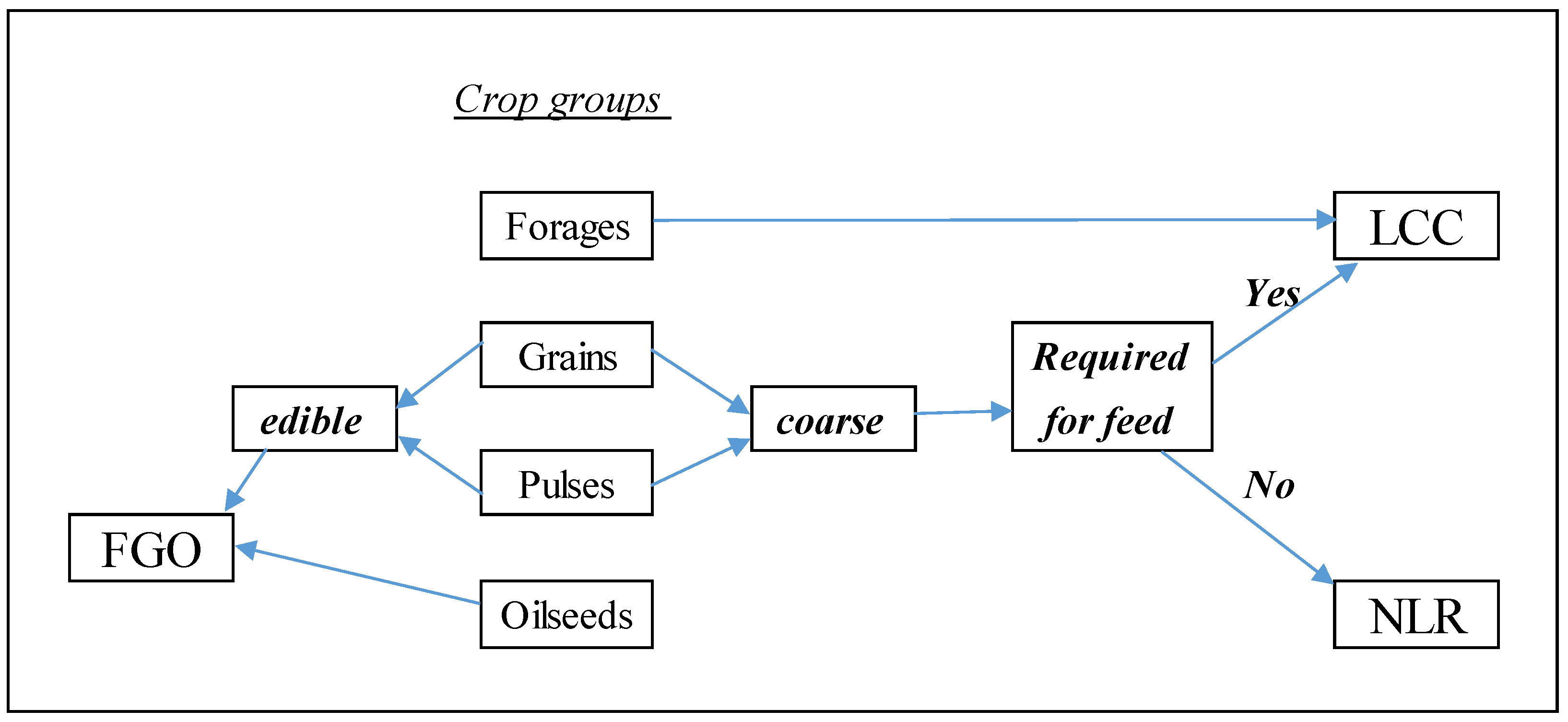
Figure 1 shows the relationships among the three land use categories and four crop groups, comprising forages, grains, pulses and oilseeds. The three land use categories are shown in the lower left (FGO), lower right (NLR) and upper right (LCC) corners of this org-chart. The first decision was whether the grains and pulses were edible (left pathway) or coarse (right pathway), meaning that they were classified as possible livestock feed crops. The second decision point was whether each crop type on the “coarse” side was needed for livestock feed. The areas needed to grow the quantity of coarse grain or pulse crop follow the “Yes” pathway to the LCC if they are required in livestock diets. The quantity that is in excess of (not required in) the livestock diet follows the “No” pathway to the NLR. Forages follow a direct path to the LCC because they were all consumed by ruminant livestock. Similarly, oilseeds follow a direct path to the FGO because of their main product being vegetable oil, even though their meal fraction may be used as livestock feed.

Coarse grains include winter wheat (Triticum aestivum), oats (Avena sativa), barley (Hordeum vulgare), grain corn (Zea mays), and other small grains. The feed pulses include dry peas (Pisum sativum) and soybeans (Glycine max). The forages include hay and alfalfa (Medicago sativa), and silage corn (Zea mays), but exclude pasture. The FGO crops include the edible grains: spring wheat (Triticum aestivum) and Durum wheat (Triticum durum), the edible pulses: lentils (Lens culinaris), chickpeas (Cicer arietinum), white beans (Phaseolus vulgaris), and colour beans (Phaseolus vulgaris), and the oilseeds: flaxseed (Linum usitatissimum), mustard seeds (Brassica juncea), sunflower (Helianthus annuus), and Canola (Brassica napus). Fall rye (Secale montanum) and sugar beets (Beta vulgaris) were also classified as FGO crops. Although soybeans, which supply both oil and livestock feed [22], appear to be an exception to the scheme in Figure 1, they were classified as feed pulses, whereby soybean oil was the by-product. As such, the inclusion of soy oil as part of the FGO would double count the soybean areas.

2.1. The Livestock Crop Complex

The role of the LCC in ULICEES was to include feed crops in livestock GHG emission calculations [6]. The original LCC application allowed the full, upstream cost of livestock products to be assessed without knowing where the land that actually grows the livestock feed was located. The limitation of the LCC concept was that it describes virtual land, and does not specify where the feed crops come from. Hence, it also does not identify which other crops may be in direct competition with the livestock feed sources. The LCC is still a useful tool in evaluating LUC, however, because, at least for livestock, it allows the interactions and competition among commodities for land to be taken into account.

To follow the LCC approach, the GHG emissions associated with growing livestock feed must be assigned to the livestock that consume that feed. But, livestock can live in EDs different from where their feed is grown. Therefore, a comparison of EDs must include the possibility of crop products being moved out of the source ED to be fed to livestock that are housed in another ED. Hence, for this analysis, the LCC assigns the GHG emissions of the feed consumed by livestock to the ED where they reside, instead of to the ED where the feed was grown. This boundary condition was needed so that livestock feed was never double counted as food for humans, since the animals that consume those crops are also consumed by humans. For each livestock type (a), the basic LCC Area (A) calculation from Population (P), diet (V) and the Yield (Y) of each feed crop (c) in ULICEES is as follows:

A_a,c = P_a × V_a,c/Y_c

(1)

The LCC area redistribution calculations at the ED scale were linked to the original ULICEES model [6]. Provincial scale feed consumption factors (F) were generated by ULICEES for 2006 for all of the feed crops in the respective diets. The provincial F factors for each livestock, a, and each crop type, c, were calculated from provincial scale A, Y and P data as:

F_a,c = A_a,c × Y_c/P_a

(2)

The terms and symbols used for these calculations are listed in

Table 1. Variables, terms and subscripts used in area redistribution calculations and weighted averages, used in each Equation Number (Eqn #) from 1 to 6.

Eqn Variables:	Term	Eqn #	Eqn Variables:	Term	Eqn #	Subscripts:	Term	Eqn #
LCC Area	A	1, 2, 3	Deficit feed	D	4	LS type	a	1, 2, 3
Population	P	1, 2, 3	Surplus feed	S	4	Crop type	c	1, 2, 3
Diet	V	1	GHG wt.	E	5	Ecodistrict	ed	4
Crop yield	Y	1, 2, 3	Product wt.	W	6	Province	prov	4
Redistribution	R	4	Binary factor	b	4	Year	y	5, 6

The Livestock (LS) type subscript, ‘a’, can represent any age-gender category for beef cattle, dairy cattle, pigs, poultry or sheep. The subscript, ‘c’ can represent any of the 7 annual feed crops included in ULICEES. The subscripts ‘ed’ and ‘prov’ indicate whether a calculation or its inputs are at the Ecodistrict or Provincial scale, respectively. The subscript, ‘y’ identifies the contribution of each year to the 3-year running averages.

.

As well as providing the basis for crop complex area calculations, the original ULICEES model [6] defined the age-gender categories in all livestock types, and provided the weight (wt) requirements for each crop in the livestock diet for all of these categories [23]. The dry matter (DM) crop yields for those crops were derived from the ICOA database. The latest published ULICEES LCC areas were only available for 2006, based on 2006 census livestock population data, and by province. Hence, the ULICEES-estimated feed consumption factors (F) from 2006 had to be extrapolated to the other years. As well, they had to be interpolated to all EDs and to the population records generated for the limited ICOA livestock categories.

2.2. Calculating the ED Scale LCC

In addition to the coefficients derived from ULICEES, the data extracted from the ICOA database for defining the ED scale LCCs were (1) areas for all farmland for those feed crops that define (i.e., are in) the LCC for all livestock types, (2) their crop yields, and (3) the livestock populations. The actual harvest weights calculated from the areas and yields from the ICOA database were an essential input to the calculations for redistributing LCC areas (described below). The LCC area calculation for each crop, c, and livestock type, a, (Table 1) in each ED was:

A_a,c = F_a,c × P_a/Y_c

(3)

For this calculation, the provincial scale livestock population data were replaced by the ED scale livestock population data provided by the ICOA database for each representative age-gender category, or set of categories, for each livestock type. ED scale crop production weights were then recalculated from the product of the yields and the recalculated crop areas for each ED and crop type.

2.3. Area Redistribution Calculations

To satisfy the “Yes” pathway to the LCC in Figure 1, the resulting ED scale LCC area estimates (needed as livestock feed) were compared to the harvested crop areas at the ED scale from the ICOA database. The total estimated LCC areas must not exceed the total harvested crop areas recorded for each province in the ICOA database. To ensure that the crop areas from the ICOA database would meet LCC feed requirements, the redistribution calculations were based on comparing crop weights, rather than areas. The crop weights calculated from LCC and livestock diets were summed over the livestock types for the feed grain and feed pulse crop groups. The random differences between the actual harvested crop weights and the LCC based crop weights had to be reconciled. The amounts by which the actual crop weights exceeded the crop weights required for the LCC, or the reverse, were calculated in each ED and crop group. The surplus weight data were then factored by a binary tag (b): where there was a surplus crop weight (actual > required), that ED was assigned a ‘1’; the ED was assigned a ‘0’ where the opposite condition was true.

The amount of surplus production to be taken from each surplus ED was proportional to that ED’s share of the total provincial surplus in that ED. That ED share ratio was converted to a required amount of feed by multiplying by the total deficit in that province. To ensure that this quantity for redistribution was only taken from surplus EDs, the binary tags (EDs with zeroes) were used to cancel out the deficit EDs from the provincial surplus calculations. By assuming that the crop weight in each deficit ED would be brought up to the required weight defined by the combined diet of all livestock types in each ED, no such calculation was needed for the deficit EDs. The redistribution function (R) was applied separately to feed grains and feed pulses. The redistributed feed weight from each surplus ED (R_ed) was calculated from the provincial deficit feed weight (D_prov), the surplus feed weight of each ED (S_ed), the provincial surplus feed weight (S_prov), and the binary tag, b (0 or 1), from Table 1 for surplus EDs (b_ed) as:

R_ed = b_ed × D_prov × S_ed/S_prov

(4)

To define the total crop weights after redistribution, the binary form of surplus ED tags (b) was used again. The weight in each ED had to be changed depending on whether that ED started with a surplus or a deficit crop weight, which could be determined from the previous three crop group summaries. Where the ED weight was in surplus, the ED amount of feed to be redistributed was subtracted from the actual harvest weight in that ED. But where the ED weight was in deficit, the required weight for the LCC was assigned to that ED. The binary sorting process determined whether the required LCC weight was taken, or the surplus weight was reduced in each ED. This process was applied separately to feed grains and feed pulses, but not to the forages, because they would only be consumed by livestock. With the exception of feed grain for the beef industry, these redistributed crop weights were ready to use in redefining the LCC crop areas. As well as defining the redistributed ED scale LCC areas, the residual surpluses defined the NLR of each ED.

2.4. Feedlots

Because of the reliance of Canadian beef production on feedlots, as well as its size and complexity, special attention will be given to the beef industry relative to the other major agricultural commodities. Beef is by far the dominant livestock industry in Western Canada, even with the decline in this industry since the mid-2000s, [24]. The beef industry offers a special challenge to the application of the LCC concept. Cattle are moved to different types of operations in their life cycles, where their diets also change [25].

The movement of slaughter cattle from ranch and backgrounding operations to feedlots, where they are fed a high grain/low roughage diet [11,25], meant an extra step in the beef analysis that was not needed for the other livestock commodities. The listings of feedlot operations in Canada published by the Canadian Cattlemen [26] gave the postal codes and the feedlot capacities (in head) for 129 feedlots for the years 2013 and 2015 in Canada. Based on these data,

Table 2. Number of feedlot operations and feedlot cattle populations (based on capacity) for each province and for Canada reported by the Canadian Cattlemen Magazine ¹ in 2013 and/or 2015.

Provinces 2	AP	QC	ON	MN	SK	AB	BC	Canada
Number of feedlots	6	2	5	14	25	75	2	129
head/feedlot	867	203	512	3074	5866	8718	3325	6654

¹, Canada’s Custom Feedlot Guide. Canadian Cattlemen—the Beef Magazine [26]. ², Provinces: AP = Atlantic Provinces, QC = Quebec, ON = Ontario, MN = Manitoba, SK = Saskatchewan, AB = Alberta, BC = British Columbia.

shows the spatial distribution of feedlot cattle populations and operations over provinces. The postal code data linked the feedlots to their ED locations, and confirmed the high concentration of feedlots in south-central Alberta [25].

Just based on the published feedlot capacities taken as an indication of the number of feedlot animals processed per year, a significant number of slaughter cattle are moved from predominantly grazing EDs to feedlots. The big cluster of feedlots in an area northwest of Lethbridge, Alberta [24] means that, even within Alberta, many feedlot cattle are moved from one ED to another. This suggests that additional quantities of grain were also moved from the EDs with no feedlots to EDs with feedlots. The weight of grain needed to feed these feedlot slaughter cattle was then moved from the redistributed grain weights. The grain consumption per head of feedlot cattle was calculated from the inputs to the provincial scale ULICEES calculations of the LCC [6]. The required provincial scale inputs were for slaughter calves, steers, and slaughter heifers, and included the populations of these age-gender categories and the weights of consumed feed grain per head in each category for 2006. Multiplying these provincial factors by the ED level feedlot capacity populations gave the weight of grain required by the feedlots in the feedlot EDs, which were then added to the grain weights in those EDs with feedlots.

To maintain the same overall weight of grain at the provincial level, proportional amounts of grain were subtracted from the EDs that did not have feedlots in a manner similar to the redistribution process used to satisfy the ED-LCC estimates. The ratios of redistributed crop weights to the actual crop weights in the EDs were the culmination of the redistribution process. Assuming that, on a per-weight of DM basis, the consumption of the five feed grains were interchangeable in livestock diets, these ratios were then used to redistribute the crop areas. The required crop areas for the LCC were subtracted from these redistributed areas to give the NLR crop areas.

2.5. Calculating GHG Emissions at the ED Scale

Whereas the ULICEES model [6] was originally aimed at just livestock and the LCC, GHG emission estimates for the FGO and NLR were required for this analysis. Fossil CO₂ emissions for growing the non-feed crops and for supplying both fertilizer and farm machinery [27,28], and barnyard energy use [29] had to be calculated for the FGO and NLR land uses. The fertilizer term by Dyer and Desjardins [28] also allowed for the minor quantities of fossil energy for pesticide production and the supply of potash and phosphate.

In contrast, CH₄ emissions were assigned directly to the livestock populations. The livestock CH₄ emission rates for each livestock type and province were imported from the original ULICEES model [6]. These imported CH₄ emission rates were adapted to the different livestock age-gender categories in the ICOA database, similar to the recalculated diet factors for the ED scale LCC calculations. To index these CH₄ emission estimates to the EDs, the ED level livestock data from the ICOA database for the LCC calculations were used.

The expanded GHG emissions budget also included the N₂O emissions from the FGO and NLR areas. Whereas N must be applied in adequate quantities to all crops, manure can be used as a substitute for commercial N fertilizer [29,30]. The assumed commercial fertilizer applications must account for the total annual sales of the commercial N fertilizer in Canada [31,32]. Manure is generally too bulky to be transported to all crops needing N applications. Hence, FGO crops would all likely receive only commercial N fertilizer. However, once on the field, manure and commercial fertilizer emit N₂O at the same rate per unit of N [30]. Hence, it was assumed that both of these N sources could be evenly distributed over all crops, regardless of whether the crops were used as livestock feed, where manure would more likely be available, or in FGO crop land without livestock. But because of the fossil energy cost of manufacturing commercial N fertilizer [28], it was still necessary to distinguish between the quantities of N from manure separately than from commercial fertilizer. The ICOA database provided the quantities of manure excreted by each livestock type in each ED. Other sources provided the total quantities of commercial N-fertilizer sold by year and province [32]. Crop-specific fertilizer recommendations [33] define the recommended N application rate, regardless of whether the source is manure or commercial fertilizer. These recommendations were the basis of distributing the commercial-manure N source differences to specific crops in order to calculate the commercial N supply energy term [28] at the ED scale.

2.6. Protein Production Dynamics

As the main product of livestock, and given the importance of livestock GHG emissions to this assessment, extra attention was given to protein. The GHG-protein indicator has been used for comparing GHG emission intensities for multiple agricultural industries and commodities [7,18], and the policy relevance of this indicator has been effectively demonstrated [6,14,15,17,34]. In this paper, protein was taken to mean the animal-equivalent protein (AeP) composed of all of the essential amino acids needed in the human diet [35]. The only non-animal derived proteins considered were those that are potential meat substitutes. From a land management basis, pulses that produce these complete proteins are currently the only plants that could potentially displace animal production to any appreciable degree from the perspective of the human diet [7]. Dyer et al. [18] calculated protein supply differently for carcass and non-carcass (milk, eggs and pulses) sources. The carcass-based calculation started with the product of live weight times the slaughter population.

Live weights: Unlike the mid-life live weights used to calculate feed consumption in the original ULICEES calculations [8,9,10,11,12,13], Dyer et al. [18] found that the live weights used to calculate protein production had to reflect the weights at the time of slaughter. Feedlot operators feed cattle destined for slaughter to a target weight of around 635 kilograms [25]. For hogs, a live weight of 117 kg for 2009 [36], was used in this analysis. The Chicken Farmers of Ontario [37] report an average bird size of 2.2 kg. For market lambs, the value used by Dyer et al. [9,17], 48 kg, was used in this new analysis.

Slaughter populations: Beef cows give birth to slightly less than a calf a year. Since the numbers of heifers retained for replacement are about equal to the culled beef cows, the beef cow population gives an approximation of the cattle sent to market from the limited age-gender data available from ICOA. A domestic farm sow averages 10 piglets per litter, and can have two to three litters per year; thus, pig farmers average about 23 piglets per year per breeding sow [38]. Honey [36] gave a similar, but slightly higher, estimate of hog reproduction rates. So a slaughter population of 24 piglets per sow was used. For broilers, 8.21 generations per year [12] was used to inflate the broiler population data from ICOA that were based on only one survey per year.

Pulses and non-carcass protein: The coefficients from Dyer and Vergé [7] for pulses is used in this analysis. Using protein-live weight conversion factors from Dyer et al. [18], the protein contents used for milk was 237 kg per cow per year [10], while for eggs, the protein content was 1.03 kg per layer per year [12].

Canola meal: In spite of being a protein source for livestock [39,40], no allowance for the feed value of canola meal was made in this analysis. With the emergence of Canola as an important industrial export crop [22,41], canola meal has become a more important component of the livestock diet. However, how much feed grains or feed pulses are being displaced by canola meal in the livestock diets is currently too difficult to determine. Also, from the perspective of land use, canola meal is a by-product of an external industry with respect to livestock production. Hence, allowing for the Canola area that provides the meal in the LCC would mean double counting Canola in the area comparisons, since this crop was already accounted for in the FGO crop areas (Figure 1).

2.7. Provincial Farm Product GHG Indicators

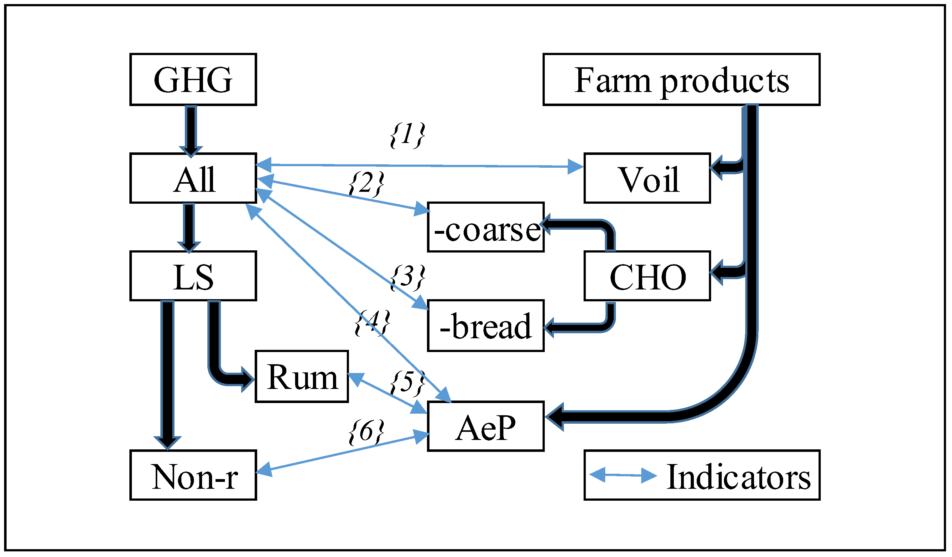
The GHG sources and the interactions with farm product groups that define the CF indicators considered in this paper are shown in Figure 2. Farm products were grouped to reflect the three nutritional components: AeP, vegetable oils (Voil), and carbohydrates (CHO). Since not all CHO is suitable for human consumption, they were separated into two groups: bread quality grains (CHO-bread), and feed grains (CHO-coarse). This distinction corresponds to the edible/coarse differentiation shown in Figure 1. As well as being a biodiesel feedstock that can reduce fossil diesel consumption and offset the global wildlife habitat and biodiversity losses associated with using palm oil as biodiesel feedstock [42], Canola was the most important Voil source in Canada.

Figure 2 also shows the hierarchy among the GHG sources. The expansion of GHG emissions beyond just livestock and the grouping of livestock as either ruminants or non-ruminants differentiated GHG emissions according to four sources: all agricultural activities (All); all Livestock (LS); ruminant Livestock (Rum); and non-ruminant Livestock (Non-r). The LS GHG emissions term is part of the All GHG emissions term, but this term is also the sum of the Rum and Non-r GHG emissions. The All category of GHG emissions was the only GHG term not fully quantified by ULICEES.

The four farm product groups in Figure 2 were assessed as possible components of CF indicators. Their spatial performance was assessed by how they varied among provinces. The reciprocal of the format used by Dyer and Vergé [7] for the GHG-protein indicator was used for Indicators 1 to 4 so that the different farm products could be compared on a common GHG emission cost basis. This basis means that each farm product was assessed against the GHG emissions from all agricultural sources in each ED, not just the GHG emissions from its own production, which facilitated inter-ED CF comparisons.

3. Results

The feedlot data set from the Canadian Cattlemen Magazine (Table 2) shows clearly that most of the feedlots, the largest feedlots, and most of the slaughter cattle are in Alberta. Saskatchewan and Manitoba are respectively, a distant second and third in these rankings. The Eastern feedlot industry is almost non-existent compared to the west. It should be cautioned that these data were for 2013 and 2015, by which time the feedlot industry had undergone a decline from the 2006 baseline year used in this analysis [24].

The livestock GHG emissions from the 2006 ULICEES simulations [7], driven by provincial census statistics, were compared with the GHG emissions from this analysis in

Table 3. Greenhouse gas emissions (GHG) from livestock estimated from provincial census data (Dyer and Vergé, 2015) and from Ecodistrict scale data for Eastern and Western Canada for 2006.

	CH4	N2O	Fossil CO2	All GHG	CH4	N2O	Fossil CO2	All GHG
			TgCO2e			TgCO2e
		From Provincial scale				From ED scale
East
Rum. 1	7.6	4.0	1.5	13.1	7.6	4.6	1.6	13.7
Non-R. 2	2.1	2.2	1.0	5.3	2.3	2.7	1.0	6.0
All LS	9.7	6.3	2.5	18.4	9.9	7.2	2.6	19.7
West
Rum.	19.4	8.5	2.1	30.1	19.4	8.1	2.5	29.9
Non-R.	2.1	1.1	0.8	4.0	2.1	1.1	0.9	4.1
All LS	21.5	9.6	3.0	34.1	21.5	9.1	3.3	34.0
Canada
Rum.	27.0	12.5	3.6	43.1	27.0	12.9	4.0	43.9
Non-R.	4.2	3.4	1.8	9.3	4.4	3.5	1.9	9.8
All LS	31.1	15.9	5.4	52.5	31.4	16.4	5.9	53.7

¹ Ruminant livestock includes dairy and beef cattle, and sheep. ² Non-ruminant livestock includes hogs and poultry.

. Since the provincial scale GHG emissions budget [7] provided a breakdown between ruminant and non-ruminant livestock, Table 3 made the same breakdown for the GHG estimates from this analysis. Most of the individual terms (for GHG type, livestock type and east-west differences) were in agreement within 0.1 to 0.5 TgCO₂e, except for the eastern N₂O, where this analysis over-estimated the Dyer and Vergé [7] value by 0.9 TgCO₂e. The ED scale GHG emission estimates over-estimated all terms from Dyer and Vergé [7], except for the western ruminant N₂O term, which seems to compensate for the relatively large over-estimation of the eastern N₂O from Dyer and Vergé [7], to give a difference nationally over all livestock and GHG types of 1.2 TgCO₂e, or a 2% over-estimation of the provincial scale ULICEES estimates.

The indicators identified as 5 and 6 in Figure 2, GHG emission intensities per unit of protein production from ruminant and non-ruminant livestock, are demonstrated in

Table 4. A comparison of the GHG-protein indicator generated at the ED scale and at the provincial scale for ruminant and non-ruminant livestock for 2006.

Input Scale:	Ecodistricts 1		Provinces 2
	Ruminants	Non-Ruminants	Ruminants	Non-Ruminants
Region:	t GHG/t protein		t GHG/t protein
East	60	18	58	19
West	99	19	110	22

¹ The Ecodistrict scale estimates were derived from the ICOA database, and integrated to Eastern and Western Canada totals. ² The Provincial scale estimates were from Dyer and Vergé, 2015.

. The intensity-based indicators for the other two nutrients (CHO and Voil) were not subjected to a similar test because they have not previously been run at the provincial scale. However, these two nutrient quantities are much easier to calculate from primary input data than protein supply, and are not affected by livestock age-gender category differences.

The two GHG-protein indicators were assessed for 2006 by comparing the east-west sums of these indicators from this analysis with the version of this indicator by Dyer and Vergé [7], which also used the ULICEES model [6]. The principle difference between the two versions was that the Dyer and Vergé [7] version was calculated with provincial inputs, whereas this analysis used ED scale inputs from the ICOA database. The GHG-protein indicator from this analysis and the Dyer and Vergé [7] paper agree to within roughly 4% in the east. The agreement was weaker in the west, with a 10% difference for ruminants and 14% for non-ruminants. However, the differences in Table 4 between the two applications of this indicator were much smaller than the differences between ruminants and non-ruminants. Although for non-ruminants, the east-west differences from this analysis were only 3%, the east-west differences for ruminants from either analysis were much larger than the differences between the two analyses.

To assess historical trends, the second goal of the paper,

Table 5. GHG emissions from all farm types (All), all livestock (LS), ruminant livestock (Rum) and non-ruminant livestock (Non-r) in Eastern and Western Canada over census years.

	All	LS	Rum	Non-r	All	LS	Rum	Non-r
		Eastern Canada				Western Canada
Years		GHG {MtCO2e}				GHG {MtCO2e}
1991	24.0	21.6	15.7	5.9	42.3	24.1	20.7	3.4
1996	23.8	21.9	15.9	6.0	50.2	28.6	24.9	3.6
2001	23.5	21.5	14.4	7.1	52.3	32.7	27.7	5.0
2006	23.2	19.9	13.3	6.5	54.7	34.1	29.1	4.9
2011	22.2	17.7	11.9	5.8	53.6	27.6	23.4	4.2

shows the GHG emissions over five census years from all farm operations and from just livestock production on an east-west basis. An appreciable amount of year to year variability was seen in the GHG emission time series between 1990 and 2013. Therefore, GHG emissions (E) for each census year (y) (Table 1) were calculated by a weighted average (ave) that took account of the years before and after each census year, as:

E_y,ave = (E_y−1 + 2 × E_y + E_y+1) / 4

(5)

The highest GHG emissions in Table 5 were for all farming operations (All) in Western Canada. The livestock GHG emissions (LS) in Western Canada were roughly 60% of the All farm type GHG emissions from all farm operations, but were also above both of the Eastern Canadian GHG time series. Unlike the All level of GHG emissions for the west, however, the western GHG emissions LS and Rum declined appreciably after 2006, reflecting a recent decline in the western beef industry. Although much smaller, the western Non-r GHG emissions did not decrease until after 2006. The eastern GHG emissions for the All category were only just above eastern GHG emissions LS category throughout the period, meaning that livestock caused almost all of the GHG emissions in the east.

Table 5 also shows the differences between GHG emissions from ruminant and non-ruminant livestock over the period defined by the five census years on an east-west basis. GHG emissions from ruminant livestock (Rum) exceeded GHG emissions from non-ruminant livestock (Non-r) in both the east and the west. Even though the Rum GHG emissions in the west declined after 2001, they still exceed the eastern Canadian GHG emissions by Rum, which have also declined steadily since 1996. The eastern Non-r GHG emissions showed little change over the period, with the eastern Non-r GHG emissions just above the western Non-r GHG emissions. In Western Canada the Rum GHG emissions were only about three to five Mt CO₂e below the LS GHG emissions throughout the period.

Table 6. The weight of Animal equivalent Protein (AeP), Carbohydrates (CHO): food quality (CHO-bread), feed or industrial use (CHO-coarse), and Vegetable oils (Voil), from Eastern and Western Canada over five census years.

	AeP	CHO-Bread	CHO-Coarse	Voil	AeP	CHO-Bread	CHO-Coarse	Voil
	Eastern Canada				Western Canada
Years	Mt{product}				Mt{product}
1991	0.7	0.1	3.0	0.1	0.4	24.2	6.9	1.9
1996	1.0	0.2	2.2	0.2	0.5	22.9	11.0	2.4
2001	1.1	0.3	2.3	0.3	0.7	16.0	6.0	2.3
2006	1.2	0.4	4.7	0.4	0.9	18.3	8.0	4.1
2011	1.4	0.3	7.1	0.5	1.0	20.2	7.0	6.6

also supports the second goal of the paper. The changes in the four main farm products in Canada over the same five census years as those used in Table 5 are shown in Table 6. Due to year-to-year fluctuations in growing conditions on the Prairies, some of the products demonstrated annual variability similar to that seen in the GHG emissions (Table 5). Thus, the quantity (weight) of each product (W) was calculated with a three year weighted average similar to the GHG emissions for the census years, as:

W_y,ave = (W_y−1 + 2 × W_y + W_y+1) / 4

(6)

The non-protein products were separated by land use, with CHO-bread and Voil coming from the FGO lands, and the CHO-coarse coming from the NLR lands. CHO-coarse was the dominant farm product in the east (first four rows), more than doubling over the period, and tripling since 1996. The CHO-bread and Voil were almost negligible in the east. Although low by weight, AeP production in the east increased steadily over the period. At least by weight, CHO-bread was the dominant farm product throughout the period in the west (Rows 5 to 8). There was less CHO-coarse produced than CHO-bread in the west. Both CHO products showed similar volatility over the period. The western and eastern protein products followed similar changes, suggesting that carcass output from the western beef industry was more stable than the CHO-coarse (mostly feed grains) changes over census years would indicate. The western Voil output showed a sharp rise from 2001, due mostly to the growth in the export market for canola.

The indicators identified as 1 to 4 in Figure 2 were quantified in

Table 7. The weight of farm products per t of GHG emissions from all farm operations in 2006, and the total GHG emission intensities for all arable land in each province for 2006: AeP = Animal-equivalent Protein; CHO = carbohydrates; bread = food quality; coarse = feed grain or industrial use; Voil = vegetable oil.

	AeP	CHO-Bread	CHO-Coarse	Voil	GHG Intensity 2
Province	kg{product}/tCO2e				tCO2e/ha
A.P. 1	23	18	58	1	4.8
Quebec	35	16	118	4	4.7
Ontario	74	21	284	28	3.2
Manitoba	22	231	64	75	2.5
Saskatchewan	19	586	268	115	1.3
Alberta	10	221	110	50	2.6
B.C. 1	25	17	7	7	8.1
Canada	28	242	165	58	2.3

¹ A.P. = Atlantic Provinces; B.C. = British Columbia. ² weight of GHG emissions per area of all annual crops and harvested perennial forages.

. These four indicators take the form of farm product weights per unit of GHG emissions (W/GHG), or GHG efficiencies. High numbers per unit of GHG emissions for one of these products indicate high GHG efficiencies in those EDs. A low product number per unit of GHG emissions can mean either a low GHG efficiency (high CF) for that product, or a diversity of production in that ED. It was not practical to show all of the spatial differences among 444 agriculturally significant EDs in Canada. Instead, the ED scale output from this analysis was spatially integrated to provincial quantities. Because the total GHG emission intensities vary among the provinces, per-ha GHG emission costs were included as a separate column in Table 7.

Saskatchewan produced the most edible plant products (CHO-bread and Voil) per unit of GHG emissions, while the most GHG-efficient producer of protein was Ontario, followed by Quebec. In the east, the protein GHG emission intensities correspond quite well with the feed grain (CHO-coarse) GHG emission intensities. For both products, Ontario was higher than Quebec, which was higher than the Atlantic Provinces. It was only in the east that the GHG efficiencies of CHO-coarse were higher than those of CHO-bread. The biggest difference between the GHG efficiencies for CHO-bread and CHO-coarse was in Manitoba, which heavily favored CHO-bread. The lowest GHG efficiencies for the total of the three plant product groups were by the two coastal regions (A.P. and B.C.). Although these two regions had relatively high GHG efficiencies for protein, they also had the highest per-ha GHG emission intensities (Column 5), particularly the west coast. The lowest GHG-efficient producer of protein was Alberta, which may partially reflect the diversity of production, since the GHG emission intensity for Alberta was close to the Canada-wide GHG emission intensity. The lowest per-ha GHG emission intensity was in Saskatchewan.

4. Discussion

On a broad regional basis, using quite simple measures, there seems to be quite good agreement between the provincial scale estimates from ULICEES [6,7] and the ED scale estimates summarized to East-West Canada totals for this assessment (Table 2 and Table 3). Some lack of agreement was to be expected because of the differences between the representative livestock age-gender categories used to import feed consumption factors from ULICEES and superimpose the ULICEES-generated LCC onto the available ICOA livestock data. The LCC area redistribution process likely increased the differences, but this effect should be small. Hence, under these caveats, the relationship between the two sets of GHG emission estimates was reasonably close.

The most meaningful evaluation of the level of agreement in Table 3 was determined by how well the two sets of protein estimates in Table 4 agreed. While the largest difference in Table 3 was in the Eastern N₂O terms, the GHG-protein intensities in Table 4 were closer in Eastern Canada than in Western Canada. The differences in the two intensity estimation methods were smaller than the east-west regional differences and the differences between the two types of livestock (ruminants vs. non-ruminants). Since the non-ruminant populations are quite small in comparison to ruminants in both the east and west, the overall performance of the GHG-protein indicator in this analysis appears to be reasonably consistent with that of Dyer and Vergé [7], and is adequate for the ruminant to non-ruminant comparison. Thus, the agreement between ED and provincial methodologies showed that the two goals of the paper were met.

This comparison did not depend on (or determine that) either or both of the methodologies being absolutely correct or accurate. The importance of this comparison was that the provincial scale ULICEES calculations were the benchmark for this model. Much of the difference can be attributed to the respective integration sequences. In the previous ULICEES applications, the input data were integrated from raw census data to provinces before they became inputs for the model calculations, whereas in this analysis, the GHG calculations were run at the ED scale and then the results were integrated to the provinces and the east-west divisions. The importance of this result was that the new estimates based on the ICOA database do not appear to introduce enough bias or distortion to alter the direction of the GHG-protein indicator output.

A guiding principle of this application of the ICOA database was to avoid double counting GHG emissions. In order to achieve this, each crop’s GHG emissions were attributed to either the crop as a food or industrial commodity or to the livestock type to which that crop is fed, but not both. The weakness of this assumption is that, when the farmers who grow feed grains sell their crops to livestock producers, the CF of the crops being sold would equal zero. On the other hand, their net product was also zero, because it was accounted for by the livestock farms on which these crops were fed to livestock. Arguably, undue effort was devoted to how to assign emissions to the feedlots, since there was no specific livestock data to verify where slaughter cattle were moved in the ICOA database.

The main goal of this paper was addressed by Table 7. To achieve this goal, the reciprocal of the GHG-protein intensity indicator used by Dyer et al. [18] and by Dyer and Vergé [7] was an essential modification for comparing commodity groups. Table 7 demonstrated that each farm product group had its own distribution across provinces. The GHG efficiencies for CHO-coarse being higher than the GHG efficiencies for CHO-bread in the east reflected the dominance of the corn-soybean complex and the dairy and pork industries in Ontario and Quebec. The dominance of Spring wheat and Canola in the Prairies was reflected in the high CHO-bread and Voil GHG efficiencies, which also account for the lowest per-ha GHG emission intensities being in Saskatchewan.

The highest GHG emission efficiencies for AeP being in Ontario and Quebec is consistent with the lower CF of dairy and pork compared to beef, as reported by Dyer et al. [18]. The AeP GHG emission efficiency for Alberta was lower than might be expected given the clustering of feedlots in that province, given the low roughage diets for feedlot cattle. This anomaly was likely due to the failure to adequately account for feedlot populations and locations by the ICOA database, and the lack of data on age-gender categories in the cattle populations at the ED scale. But it might also stem from the feedlot cattle being closer Non-r than Rum livestock with respect to GHG emissions (particularly CH₄), due to their low roughage diet. The decline in the Rum GHG emissions after 2006 (Table 5), while western Protein production continued to increase (Table 6), could be the result of shifts in beef diets to less forage and more of the increasingly available canola meal [40], and/or a displacement of beef by pork. The steady increase in protein production in the east (Table 6) was most likely a result of an increasingly efficient dairy industry and a dairy population stabilized by supply management [43].

Although the suite of ED scale indicators was only shown for one year (Table 7), the basis for applying Indicators 1 to 4 from Figure 2 to other years (the second goal of the paper) can be demonstrated from Table 4 and Table 5. For example, there was a sharp rise in CHO-coarse production in Eastern Canada from 2001 to 2011 (Column 3 of Table 6), along with relative stability in the All category of GHG emissions (Column 1 of Table 5) in the east. This suggests that Indicator 2 would show an appreciable increase over this period. For Western Canada, in spite of the relative stability in the All category of GHG emissions (Table 5), the results from Table 6 for the west suggest that after 1996 Indicators 1, 2 and 4 would all increase while Indicator 3 would fluctuate without any clear trend during the period in the west.

5. Conclusions

With 444 agriculturally significant EDs in Canada, it was not practical to show any ED comparisons in this paper. However, a basis for such comparisons has been established. The GHG emissions budget of a whole ED area would have to cover whatever FGO, NLR and LCC croplands are in that ED, instead of individual farms or specific commodities. To avoid double counting of GHG emissions, no area in any ED can be assigned to more than one land-use category. The NLR is a direct residual from the LCC determinations. Furthermore, the LCC in any ED may include cropland from another ED, while also including the GHG emissions from any livestock it housed. A future improvement should be to better calibrate the crop weight/area adjustments for feedlot feed use if additional feedlot diet data can be gathered, including better data on the number of feedlots, and their locations and populations. Acquiring such data would require a direct dialogue with the feedlot operators, with the most likely mode of communication being focus groups. But the algorithm for the adjustment described in this paper should still be applicable.

By accounting for the age-gender categories and the GHG emissions associated with their feed sources and housing of each livestock type [6], ULICEES defined many aspects of the life cycles of these five GHG emission budgets [9,10,11,12,13]. Although this analysis added some increased spatial precision to the movement of the livestock feeds, it did not attempt to improve on these life-cycle functions. It was intended to be a spatial interpolation of these functions, not a stand-alone life-cycle assessment of Canadian livestock production. Since there was no allowance in this paper for changes in soil carbon, another future development should be to investigate the use of the payback period concept used in the ULICEES model [6] to link the CF to the sequestering or discharging of the soil carbon sink.

An important side benefit of this analysis was to demonstrate that ULICEES calculations could be adapted to operate at the ED scale. In some respects, the version of the ULICEES model developed and used in this paper was a meta-model of the original ULICEES [6]. But in addition, ULICEES was only a part of the agricultural GHG emissions model developed in this paper because the ED scale CF included crops and croplands not in the livestock diets. This expansion should be an important new tool in LUC and GHG reduction policy measures, because it demonstrates the hierarchy among the four levels of GHG budgets involved in Canadian agriculture (All, LS, Rum and Non-r (Figure 2)). These four GHG emission levels, together with the three land use categories (Figure 1), provide a unique perspective on the overall CF of Canadian agriculture. The implications for LUC include the encroachment of industrial crops, such as malting barley or biodiesel feedstock, on land used previously for food crops or livestock feed [16]. Also, the almost complete dependence of non-ruminants and beef feedlots on feed grains puts these industries in direct competition with biofuel feedstock production [14,15].

By identifying the EDs in which the LCC areas actually belong, this paper went a step further than the provincial scale ULICEES. However, the techniques for redistributing crops among EDs based on their production and use should be a useful tool for assessing future or current LUC. This process should be applicable to land units defined at scales other than EDs, if appropriate crop and livestock data are available for those land unit scales. Because many countries may not have the equivalent of the Canadian ICOA database, they may not be able to apply the methodology described in this paper exactly as it was applied in Canada. The GHG redistribution process that was applied to EDs in Canada could be applied to a set of administratively defined districts that do not necessarily have agro-ecological uniformity with their boundaries. The LCC is also not just an abstract concept limited to units of virtual land. Instead, the LCC is a tool by which the CF of livestock feed can be reallocated from source growing areas to the land units in which livestock are housed, and at a local scale. Without the LCC approach (reallocating feed crops from where-grown to where-consumed), the distribution of GHG emissions among the four GHG emission levels (defined in Figure 2) would likely have been quite different than presented in this paper.

Of the six indicators introduced in Figure 2, the first four were quantified in Table 7, whereas the last two were quantified in Table 4. Indicators 5 and 6 demonstrate how indicators can be used to monitor GHG emission intensity differences between two commodity groups. For this role, the indicator is best served by a CF estimate based on the same commodity and that includes only the GHG emissions from that commodity. Indicators 1 to 4 (Figure 2) illustrate a better approach to integrating the multi-product impacts on an individual land unit, thus facilitating inter-ED comparisons. These four efficiency indicators used a single GHG emission estimate that includes all of the GHG emitted from each land unit.

The reciprocal format used for the indicators in Table 7 tackle a very complex set of relationships among Canadian farm products and land uses. Firstly, the product groups cannot be compared in terms of their value or total weights. For example, while the weights of protein production are much smaller than those of either CHO product group, protein has a crucial role in the human diet. Secondly, of the three plant product groups, only CHO-bread has a direct, dedicated role in the human food supply. Thirdly, livestock production, as reflected in protein production, has a much greater CF than plant products. But simply shifting farm production away from livestock is currently not a readily available policy option for reducing the CF of Canadian agriculture, as long as the global market for animal products is stronger that the market for edible grains. Finally, the true GHG emission cost of increasing Canola areas (the main Voil product) must account for the impact on other land uses and on the CF of the agriculture sector. The application of CF indicators to the ICOA database, as described in this paper, provides an approach to answer these four LUC questions at a district or regional scale.

There are some possible future scenarios confronting Canadian agriculture for which Indicators 1 to 4 could provide important policy guidance. The dramatic growth in Canola in Western Canada [41] is likely to continue. The recent decline in the beef industry [24] is also likely to continue. If the continuation of supply management which underpins the Canadian dairy industry [43] is threatened by future trade agreements, this industry may also see a major decline. Since the impacts of these and other potential changes may vary considerably even within provinces, an accurate tracking of the CF of Canadian agriculture would require the ED scale spatial precision provided by the methodology described in this paper.