Tools for Optimizing Management of a Spatially Variable Organic Field

Abstract

Geostatistical tools were used to estimate spatial relations between wheat yield and soil parameters under organic farming field conditions. Thematic maps of each factor were created as raster images in R software using kriging. The Geographic Resources Analysis Support System (GRASS) calculated the principal component analysis raster images for soil parameters and yield. The correlation between the raster arising from the PC1 of soil and yield parameters showed high linear correlation (r = 0.75) and explained 48.50% of the data variance. The data show that durum wheat yield is strongly affected by soil parameter variability, and thus, the average production can be substantially lower than its potential. Soil water content was the limiting factor to grain yield and not nitrate as in other similar studies. The use of precision agriculture tools helped reduce the level of complexity between the measured parameters by the grouping of several parameters and demonstrating that precision agriculture tools can be applied in small organic fields, reducing costs and increasing wheat yield. Consequently, site-specific applications could be expected to improve the yield without increasing excessively the cost for farmers and enhance environmental and economic benefits.

1. Introduction

Wheat (Triticum turgidum var. durum) is cultivated over more than 13 million hectares worldwide [1]. In recent years, the management regime of those crops has undergone a series of changes as a result of an increase in average field size. New tools are consequently required to enable a global view of these larger-sized fields and to determine the heterogeneous zones that often appear within them. The use of yield prediction maps is an important tool for the delineation of within-field management zones.

Yield prediction maps are of great importance to ensure that yields are maximized with fewer inputs, less waste and consequently less environmental impact. Accurate estimation of yield can be used for zonal management of the most productive areas, to plan the best time for harvesting and its transport for industrial processing, and to locate any water and nutritional deficiencies in the field [2]. Yield monitoring and mapping have given producers a direct method for measuring spatial variability in yield [1]. Along with yield mapping, producers have expressed increased interest in characterizing soil variability.

Wheat yield is spatially variable because of inherent spatial variability of factors affecting the yield at field scale [3]. Precision agriculture is an emerging management strategy that combine geographic information systems (GIS), global positioning systems (GPS), computer modeling, remote sensing, expert systems, and advanced information processing with the goal of optimizing returns on inputs while preserving resources [4].

Precision agriculture can provide a knowledge-based management of agricultural production to reduce environmental impact and increase profit margins [5]. According to Virgilio et al. [6], the core of precision farming theory is to understand field spatial variation and the relations with crop response, resulting in a substantial increase in the input effectiveness and in the average biomass yield and obtaining economic and environmental benefits. Precision agriculture in conventional agriculture is already recognized, although it is uncommon to see similar research in organic agriculture because of the high heterogeneity of the plant production factors and yield [7].

The yield variability is not an independent phenomenon, and in theory, it should be influenced by the soil variability and by the scarcest resource that controls the growth and not by the sum of all resources available [8]. However, in the field, many production factors conjointly act, and some positive effects may be hidden by the negative ones, such as low water content [9]. GIS is a powerful tool for analyzing spatial data and establishing a process for decision support [10]. Geostatistics offers the possibility to represent the spatial dependence of soil and yield variable distribution [11].

The approach of precision agriculture generates an intensive stream of data, ranging from soil parameters to yield factors that need to be submitted to data mining methodologies so that concrete relations of the several factors influencing the yield can be shifted from the raw data. Raster maps with detailed information on soil properties and yield components have some degree of correlation; thus, principal component analysis can group them in a new and reduced set of images that can be more easily analyzed and understood [12].

Therefore, the present research addresses the following: (i) to estimate the spatial variation of durum wheat yield under organic agriculture field conditions, (ii) to assess the spatial variation of soil properties, (iii) to produce thematic maps of yield and soil parameters using geostatistical kriging approaches to find possible relations between soil parameters and yield, and (iv) to reduce the level of complexity between the measured parameters using principal component analysis.

2. Materials and Methods

2.1. Study Area

The study area was located in the organic farm of Kibbutz Nirim (34°35′ N/31°20′ E) in the North of the Negev Desert in Israel. Average temperature varies between 16 °C in January and 27 °C in August. The average annual rain is 250 mm, and the annual evaporation from class A pan is 1550 mm (30 years of meteorological data). The soil is Loess (Calcic haploxeralf) with an average bulk density of 1320 kg/m³ and pore volume of 0.5 m³/m³; clay, silt, and sand are 150, 300, and 550 g/kg, respectively. The texture is sandy loam, and the cation exchange capacity is 18 cmol/kg.

The research field was in cultivation during data collection and was sowed with wheat (Triticum turgidum var. durum Desf.) on January, which is usual sowing time in Negev Desert, and harvested on 10 June 2004. The grid used to gather the samples followed the characteristics of the yield and was designed in a triangular way, with the objective of maximizing the covered area with the minimum number of samples, fitting the field with 73 samples, an amount in concordance with other studies and authors [13]. In precision agriculture, the rule is to use sampling intervals equal to half of the semivariogram range [14]. To know the optimal grid size, “cross validation” was used to compare the prediction performances of the semivariograms [15]. This grid fitted an area of 1.9 ha, which is enough for a precision agriculture study according to previous studies [16]. Each grid point was determined in the field by the use of GPS.

Soil samples were collected during the emergence at February 17, at 15 March and at 6 June 2004. Those dates represent the initial, middle, and final stages of crop growth prior to harvesting. Soil specific area (SSA), nitrate, soil water content (SWC), and carbon flow (CF) were determined in the upper 0.15 m. SSA was measured with the Ethylene Glycol Monoethyl Ether method [17], nitrate with Ion Specific Probe [18] and SWC with gravimetric method as was described by Gardener [19] using 100 gr of soil measured for their initial and final mass after being dried for 24 h in a 110 °C oven. Measurement of the soil carbon flux was performed using the LI-6400 Soil CO₂ Flux system, which is an InfraRed Gas Analyzer (IRGA) working in a closed system chamber [20]. Measurements were performed several days after harvest. A PVC ring, buried at a depth of about 1 cm, was placed at each sampling point. The LI-6400 gas chamber was then placed on each ring and the soil carbon flux was measured.

Before harvesting of wheat field, yields at the 73 predetermined georeferenced points were measured using the total number of grains and plants, the weight of 1000 kernels as well as the total weight of grain, average weight of one kernel, stems, plants, and grain/plant were determined in a sampling area of 0.2 m² per point [21]. The leaf area index (LAI) measurements were determined only at the two initial dates and were not measured on the last date because the crop was completely dry. LAI was measured with the ΔT—SunScan Canopy Analysis System as described by Welles and Norman [22].

2.2. Data Transformation and Trend Removal

The gathered data were checked for skewness, and data transformation functions of log(x), sqrt(x), inv(x), and sq(x) were applied to bring the skewness closer to zero [23]. After the data were checked for trend using the mean-polish trend removal method [24,25]. This method divides the grid system of the sample into columns and rows and tests for an increase or decrease of data values. The Z(x)−m−r_k−c_l (residual) and (k−k)(l−l) were calculated. The m is the overall mean; r and c are the row and column mean, respectively; and k and l are the mean of number of rows and columns. The values of Z(x)−m−r_k−c_l and (k−k)(l−l) were plotted, and trend line was fitted.

For each parameter, the trend line was tested for slope using an analysis of variance (ANOVA) with F distribution table [26]. A slope equal to zero indicated that there was no trend, whereas a value different from zero indicated a trend in the data. If the ANOVA proved that there was a parameter with trend, then the residual values were used instead of the measured values for the interpolation because residuals are correlated even if the observations are not.

2.3. Interpolation Method

The interpolation method used for raster creation was ordinary kriging, which is a common method for data interpolation [27]. This method is based on the creation of a semivariogram graphic and from the information contained in the best-fitted model [28,29].

The models used were gathered from common geostatistics publications [30,31]. The semivariogram is a plot between the distances of ordered data and their value of semi variance; this plot explains the spatial relation between the samples and is given by Equation (1).

$$\gamma \left(h\right)=\frac{1}{2\text{N(h)}}{\displaystyle \sum {\left[Z_i-Z_{i+h}\right]}^2}$$

(1)

The most related samples have lower values of semi variance (γ(h)). N(h) is the number of samples that can be grouped using vector h, Z_i represents the value of the sample, and Z_i+h is the value of another sample located at a distance h from the initial sample Z_i. The semivariogram is a point graphic with points plotted at specific distance intervals. Because there is a need to know the semi-variance value at distances not defined in the plot, a model was fitted using the lowest possible root square error.

The fitted model provided two important parameters to determine if the samples are spatially correlated, which were the Nugget (N) and Sill (S). The “nugget/sill ratio” (N/S) was introduced by Cambardella et al. [32] as a measure to quantify the level of spatial structure. A low N/S ratio (<0.25) indicates that the samples are spatially correlated, while a high N/S ratio (>0.75) means that the samples have a very low spatial correlation.

According to Issaks and Srivastava [31], kriging tries to have a mean residual error equal to zero with the lowest possible value of the standard deviation of the error and, at the same time, estimates the weighted linear combinations (wi) of the available data for the interpolation result (Equation (2)).

$$z(x_0)={\displaystyle \sum _{i=1}^n{w}_i}\hspace{0.17em}.\hspace{0.17em}z(x_i)\hspace{1em}\hspace{1em}\wedge \hspace{1em}\hspace{1em}{\displaystyle \sum _{i=1}^n{w}_i}=1$$

(2)

The linear weight necessary for the interpolation is obtained by the ordinary kriging system (Equation (3))

$$\begin{array}{c}\hspace{0.17em}\hspace{0.17em}\hspace{1em}\hspace{0.17em}\hspace{1em}C\hspace{1em}\text{.}\hspace{1em}w\hspace{1em}=\hspace{0.17em}D\\ \left[\begin{array}{llll}{C}_{11}\hfill & \cdots \hfill & C_{1\text{n}}\hfill & 1\hfill \\ ⋮\hfill & \ddots \hfill & ⋮\hfill & \cdots \hfill \\ C_{n1}\hfill & \cdots \hfill & C_{nn}\hfill & 1\hfill \\ 1\hfill & \cdots \hfill & 1\hfill & 0\hfill \end{array}\right]\hspace{1em}\text{.}\hspace{1em}\left[\begin{array}{l}{w}_1\hfill \\ ⋮\hfill \\ w_n\hfill \\ \mu \hfill \end{array}\right]\hspace{1em}=\hspace{1em}\left[\begin{array}{l}{C}_{10}\hfill \\ ⋮\hfill \\ C_{n0}\hfill \\ 1\hfill \end{array}\right]\hspace{1em}\\ \hspace{1em}\left(n+1\right)\ast \left(n+1\right)\hspace{1em}\hspace{0.17em}\hspace{1em}\hspace{1em}\left(n+1\right)\ast 1\hspace{1em}\left(n+1\right)\ast 1\end{array}$$

(3)

The matrix C contains the covariance from all the samples surrounding the sample to be interpolated. The matrix w contains the weights as well as the parameter called Lagrange parameter. The matrix D contains the covariance from the sample to be determined and the surrounding ones. The final objective is to determine matrix w.

2.4. Principal Component Analysis

Principal component analysis (PCA) is a linear transformation of a set of numerical variables (or images), which creates a new variable set (or images), called principal components (PCs). In this framework, the new variables are uncorrelated and ordered in terms of the amount of variance explained from the original data [33]. The advances made in the last years concerning PCA and image analysis can be useful when there is sufficient spatial information in agricultural fields, mainly, raster images that can be generated by sampling and interpolation using geostatistics [34,35].

Each PC is a combination of the original images with coefficients equal to the eigenvector of the covariance matrix [36]. Aside from the eigenvector, the eigenvalues are also obtained and can be used to determine how well the PC can explain the variability of the original values. It can therefore be useful in determining the number of PCs necessary for in-depth analysis.

To begin the transformation, a covariance matrix $\overrightarrow{C}$ of the original data has to be found. Using the covariance matrix, the eigenvalues ${\text{λ}}_i$ and the eigenvectors ${\overrightarrow{e}}_i$ are obtained from the following equation (Equation (4)).

$$\left|\overrightarrow{C}-{\lambda }_i\overrightarrow{I}\right|=0\hspace{1em}\equiv \hspace{1em}\left(\overrightarrow{C}-{\lambda }_i\overrightarrow{I}\right)\hspace{0.17em}{\overrightarrow{e}}_i=0$$

(4)

where i ϵ [1,2,3….n], n is the total number of images, and $\overrightarrow{I}$ is the identity matrix. The PC images are then given by Equation (5):

$$\overrightarrow{P}C=\overrightarrow{T}\hspace{0.17em}°\hspace{0.17em}DN$$

(5)

where $\overrightarrow{D}N$ is the digital number matrix of the original images and $T$ is the transformation matrix given by Equation (6):

$$\overrightarrow{T}\hspace{1em}\equiv \left[\begin{array}{lll}{e}_{11}\hfill & \cdots \hfill & e_{1\text{n}}\hfill \\ ⋮\hfill & \ddots \hfill & ⋮\hfill \\ e_{n1}\hfill & \cdots \hfill & e_{nn}\hfill \end{array}\right]$$

(6)

where e_nm is the value of the values of the eigenvectors.

The generated PC images are uncorrelated. The transformed data points are linear combinations of their original data values weighed by the eigenvectors. The percentage in each of the components is given by the next equation (Equation (7)).

$$Varianc{e}_i=\frac{{\text{λ}}_i\ast 100}{{\displaystyle \sum _{i=1}^n{\text{λ}}_i}}$$

(7)

where ${\text{λ}}_i$ is the calculated eigenvalues obtained in Equation (4).

By computing the correlation of each original band with each PC, it is possible to determine how the images (and therefore, the parameters that they represent) are associated with each principal component. This enables determining which of the actual variables are more important, as well as the relation between them. One of the contributions of this study was the conversion of PCs into actual variables.

The variables required for the calculation of the correlation between the map and a PC are as allows: the eigenvalue (${\lambda }_i$), the variance of the image ($Va{r}_i$), and the eingenvector value for image i and component p ($e_{ip}$) (Equation (8)).

$$R_{ip}=e_{ip}\frac{\sqrt{{\lambda }_i}}{\sqrt{Va{r}_i}}$$

(8)

GRASS (Geographic Resources Analysis Support System) and R software were used as tools for the present study. For the spatial analysis and semivariogram creation it was used the “sgeostat” software (Iowa State University). The initial data were imported from the spreadsheet (after it was processed for trend and skewness), using a comma-separated value (CSV) file format. For the semivariogram estimation, a lag of 10 and a maximal range of 100 were used. The lag and range values were obtained after several simulations of estimated semivariogram creation. For interpolation and export to GRASS, it was necessary that R run from inside GRASS so that the spatial information of the study area can be imported to R (projection, grid resolution, mask, etc.) and then be exported and integrated on the GRASS database [37].

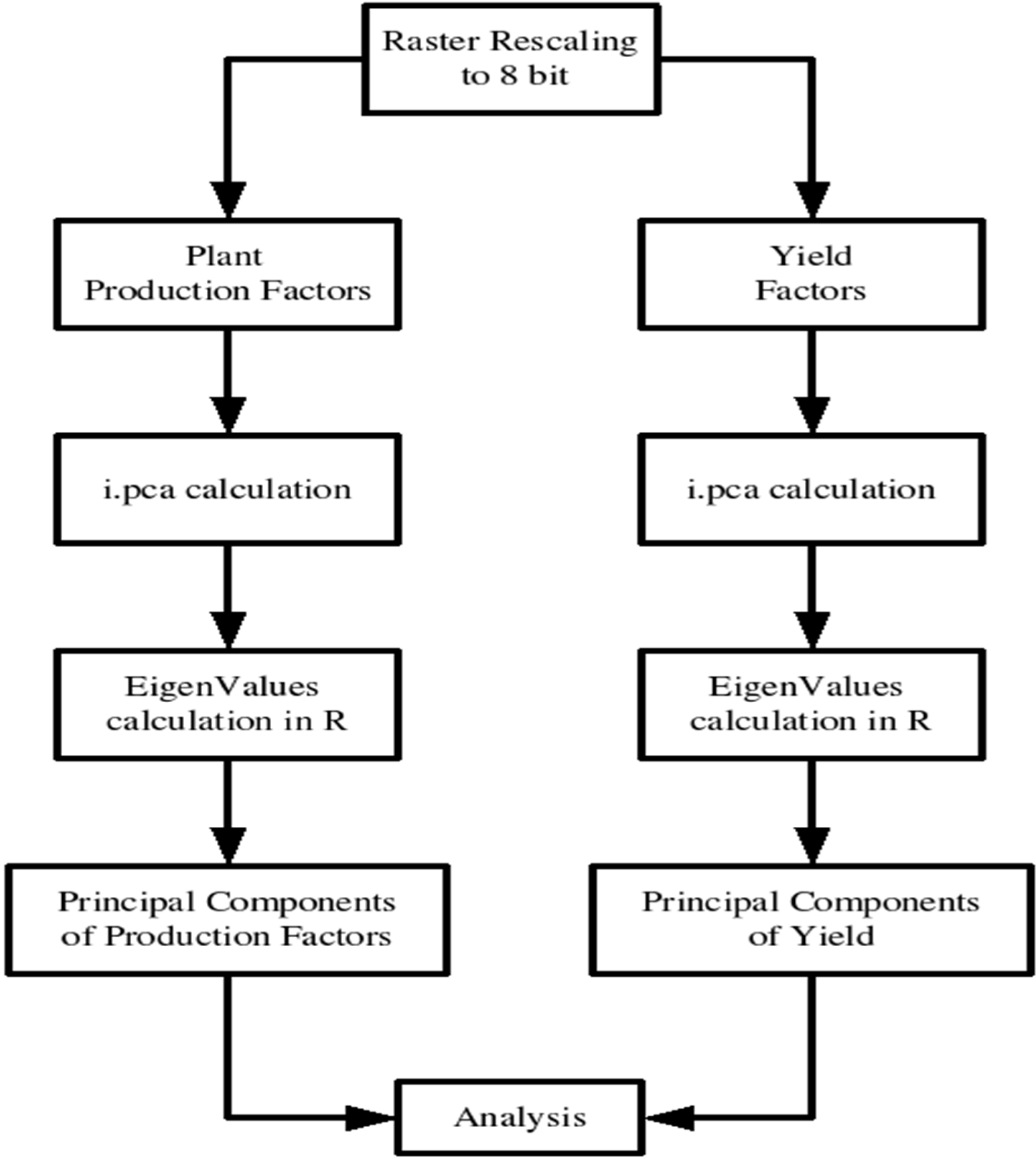
Figure 1 presents the flowchart describing the PCA calculation methodology using the raster maps produced from geostatistics. The raster images created with geostatistics were imported from R software and rescaled from their original values to an 8-bit scale using the module r.rescale. At the rescale, the minimal interpolated value represented by 0 digital number (DN) and the maximal interpolated value was represent by 255 DN. This rescale was necessary to confirm all the rasters and to ease their analysis [38]. For the PCA calculation, the i.pca module was used; this module processes n input raster map layers and produces n output raster map layers containing the principal component in decreasing order of variance and also output of the eigenvector matrix.

Afterward, the raster images were separated into the two groups of plant production factors and yield factors. For each group, a PCA was conducted, obtaining the PC rasters and the eigenvector. To calculate the eigenvalues, the covariance array was passed to R software and using the eigenfunctions, the eigenvalues were obtained. From Equation (8), it was determined which factor contributed the most for each of the principal components because the most important factors will have the highest correlation with the principal component to where they belong.

Figure 1. Flowchart describing the PCA calculation methodology using the raster maps produced from geostatistics.

Figure 1. Flowchart describing the PCA calculation methodology using the raster maps produced from geostatistics.

3. Results

The trend analysis revealed that only the nitrate recorded on February 17 had a trend for a 10% confidence interval. This parameter was detrended, and the residuals were used for the semivariogram creation and interpolation. The majority of the parameters had a moderate-strong or moderate-weak spatial correlation (Table 1). The number of plants had a null spatial relation between samples, which was caused by the random sowing procedure.

Table 1. Basic statistics of the parameters, results of the semivariograms, and spatial dependence.

Parameter	Min.	Max.	Mean	CV	SK	Nugget	Sill	Range (m)	Model	N/S	Spatial Dep.
Soil specific area (m2/g)	67.5	104.7	82.17	11.12	0.51	7.94 × 10−7	1.86 × 10−6	50	spherical	0.43	Moderate
Nitrate in February (ppm)	2.78	22.83	5.94	52.9	2.82	1.22 × 10−3	4.83 × 10−3	15.85	exponential	0.25	Mod.-strong
Nitrate in March (ppm)	2.92	16.67	6.01	39.96	1.89	2.42 × 10−3	3.60 × 10−3	64.25	exponential	0.67	Mod.-weak
Nitrate in June (ppm)	2.39	20.16	5.25	58.31	2.17	0.01	0.02	796.2	exponential	0.48	Moderate
SWC in. February (%)	6.92	11.99	10.21	9.47	−0.55	131.19	388.02	11.88	exponential	0.34	Mod.-strong
SWC in March (%)	6.99	11.99	10.16	9.48	−0.39	239.74	394.7	39.33	exponential	0.61	Mod.-weak
SWC in June (%)	1.91	6.97	4.03	24.52	0.78	0.02	0.06	10.79	exponential	0.35	Mod.-strong
Carbon flux (μmol m−2·s−2)	0.16	2.35	0.96	47.06	1.08	0.19	0.22	48.59	exponential	0.88	weak
LAI in February	1.3	4.2	2.56	26.14	0.41	0.02	0.05	43.14	exponential	0.3	Mod.-strong
LAI in March	2	4.6	3.55	20.42	−0.62	7.06	24.45	13.76	exponential	0.29	Mod.-strong
Number of grains	430	1247	713.2	21.44	0.27	4.91	9.41	59.75	spherical	0.52	Moderate
Number of plants	7	36	20.4	33.17	0.33	0.55	—	—	nugget	—	None
Weight of 1000 grains (g)	31.67	72.49	53.42	12.73	−0.6	1.00 × 10−6	494634	6.58	exponential	0.00	Strong
Total weight of grain (g)	22.22	56.87	37.68	20.07	−0.06	48.56	69.72	158.64	spherical	0.69	Mod.-weak
Weight of kernel (g)	8.85	42.18	19.63	40.46	1.08	0.05	0.2	48.89	exponential	0.25	Mod.-strong
Weight of stems (g)	6.74	58.52	24.95	48.78	0.8	0.66	1.39	12.01	exponential	0.48	Moderate
Weight of plants (g)	22.22	56.84	37.68	42.43	0.92	0.08	0.18	19.08	exponential	0.42	Mod.-strong
Weight grain/plant (g)	0.31	2.4	0.99	43.34	0.68	0.08	0.22	60.69	spherical	0.35	Mod.-strong

Table 1. Basic statistics of the parameters, results of the semivariograms, and spatial dependence.

Parameter	Min.	Max.	Mean	CV	SK	Nugget	Sill	Range (m)	Model	N/S	Spatial Dep.
Soil specific area (m2/g)	67.5	104.7	82.17	11.12	0.51	7.94 × 10−7	1.86 × 10−6	50	spherical	0.43	Moderate
Nitrate in February (ppm)	2.78	22.83	5.94	52.9	2.82	1.22 × 10−3	4.83 × 10−3	15.85	exponential	0.25	Mod.-strong
Nitrate in March (ppm)	2.92	16.67	6.01	39.96	1.89	2.42 × 10−3	3.60 × 10−3	64.25	exponential	0.67	Mod.-weak
Nitrate in June (ppm)	2.39	20.16	5.25	58.31	2.17	0.01	0.02	796.2	exponential	0.48	Moderate
SWC in. February (%)	6.92	11.99	10.21	9.47	−0.55	131.19	388.02	11.88	exponential	0.34	Mod.-strong
SWC in March (%)	6.99	11.99	10.16	9.48	−0.39	239.74	394.7	39.33	exponential	0.61	Mod.-weak
SWC in June (%)	1.91	6.97	4.03	24.52	0.78	0.02	0.06	10.79	exponential	0.35	Mod.-strong
Carbon flux (μmol m−2·s−2)	0.16	2.35	0.96	47.06	1.08	0.19	0.22	48.59	exponential	0.88	weak
LAI in February	1.3	4.2	2.56	26.14	0.41	0.02	0.05	43.14	exponential	0.3	Mod.-strong
LAI in March	2	4.6	3.55	20.42	−0.62	7.06	24.45	13.76	exponential	0.29	Mod.-strong
Number of grains	430	1247	713.2	21.44	0.27	4.91	9.41	59.75	spherical	0.52	Moderate
Number of plants	7	36	20.4	33.17	0.33	0.55	—	—	nugget	—	None
Weight of 1000 grains (g)	31.67	72.49	53.42	12.73	−0.6	1.00 × 10−6	494634	6.58	exponential	0.00	Strong
Total weight of grain (g)	22.22	56.87	37.68	20.07	−0.06	48.56	69.72	158.64	spherical	0.69	Mod.-weak
Weight of kernel (g)	8.85	42.18	19.63	40.46	1.08	0.05	0.2	48.89	exponential	0.25	Mod.-strong
Weight of stems (g)	6.74	58.52	24.95	48.78	0.8	0.66	1.39	12.01	exponential	0.48	Moderate
Weight of plants (g)	22.22	56.84	37.68	42.43	0.92	0.08	0.18	19.08	exponential	0.42	Mod.-strong
Weight grain/plant (g)	0.31	2.4	0.99	43.34	0.68	0.08	0.22	60.69	spherical	0.35	Mod.-strong

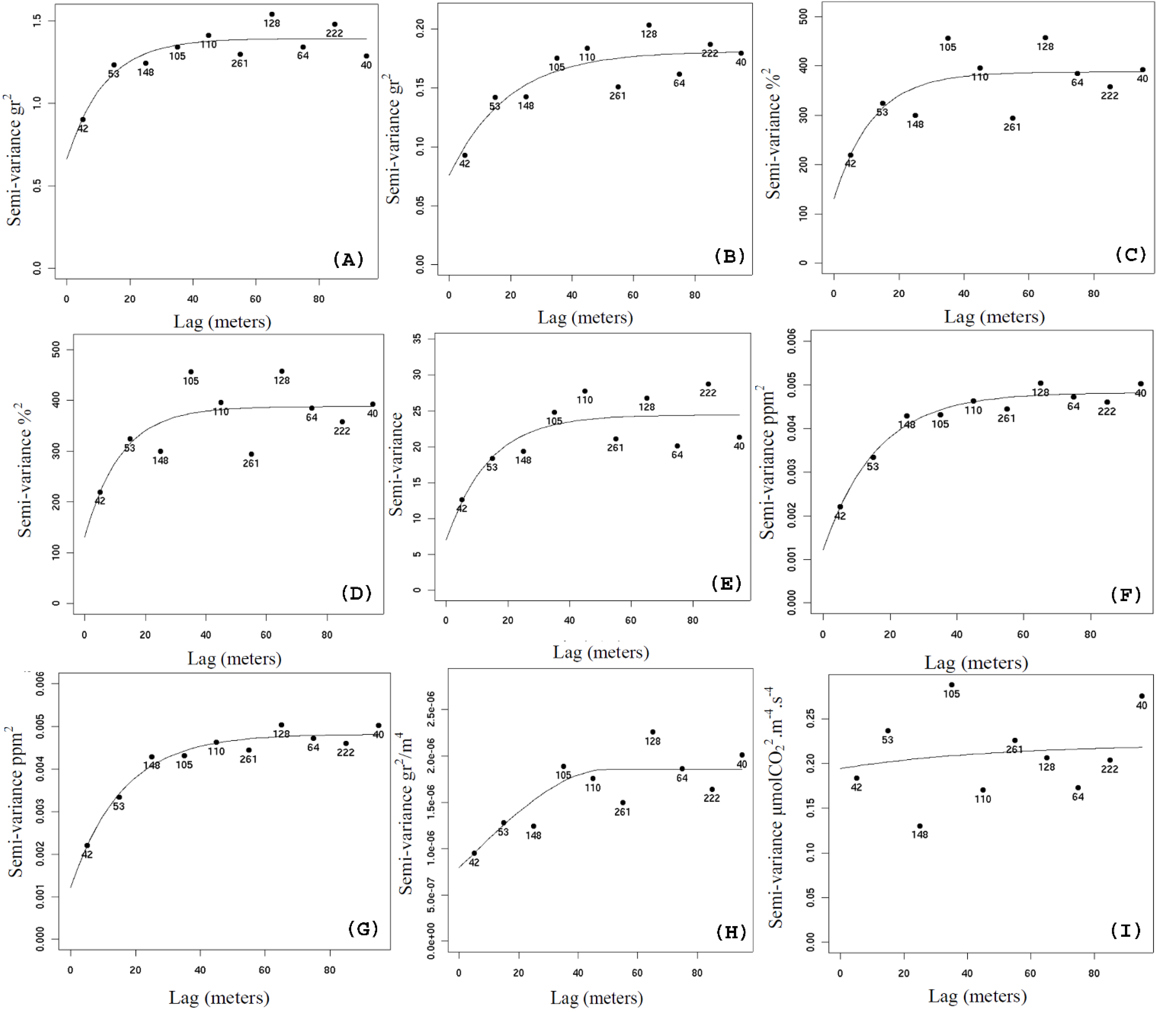
Figure 2 shows the semivariograms of the main parameters studied. The parameter weight of stems is moderate-strong spatial correlated with semi-variogram showing a spatial range below 20 meters. The parameter weight of plants is moderate-strong spatial correlated, but despite the slow increase of the sill of the model, the majority of the spatial correlation is on the first three bins, which is a range a bit over 20 meters. The semivariogram for Nitrate on February 17, which is the only parameter that has shown a non-stationary behavior, shows a very good model fitting.

Figure 2. Results of semivariogram and model fitting for the parameter weight of stems (A); weight of plants (B); the soil water content recorded in February 17 (C); the soil water content recorded in June 6 (D); leaf area index recorded March 15 (E); Nitrate in February 17 (F); SSA (G); total weight of grain (H); Carbon flux (I).

Figure 2. Results of semivariogram and model fitting for the parameter weight of stems (A); weight of plants (B); the soil water content recorded in February 17 (C); the soil water content recorded in June 6 (D); leaf area index recorded March 15 (E); Nitrate in February 17 (F); SSA (G); total weight of grain (H); Carbon flux (I).

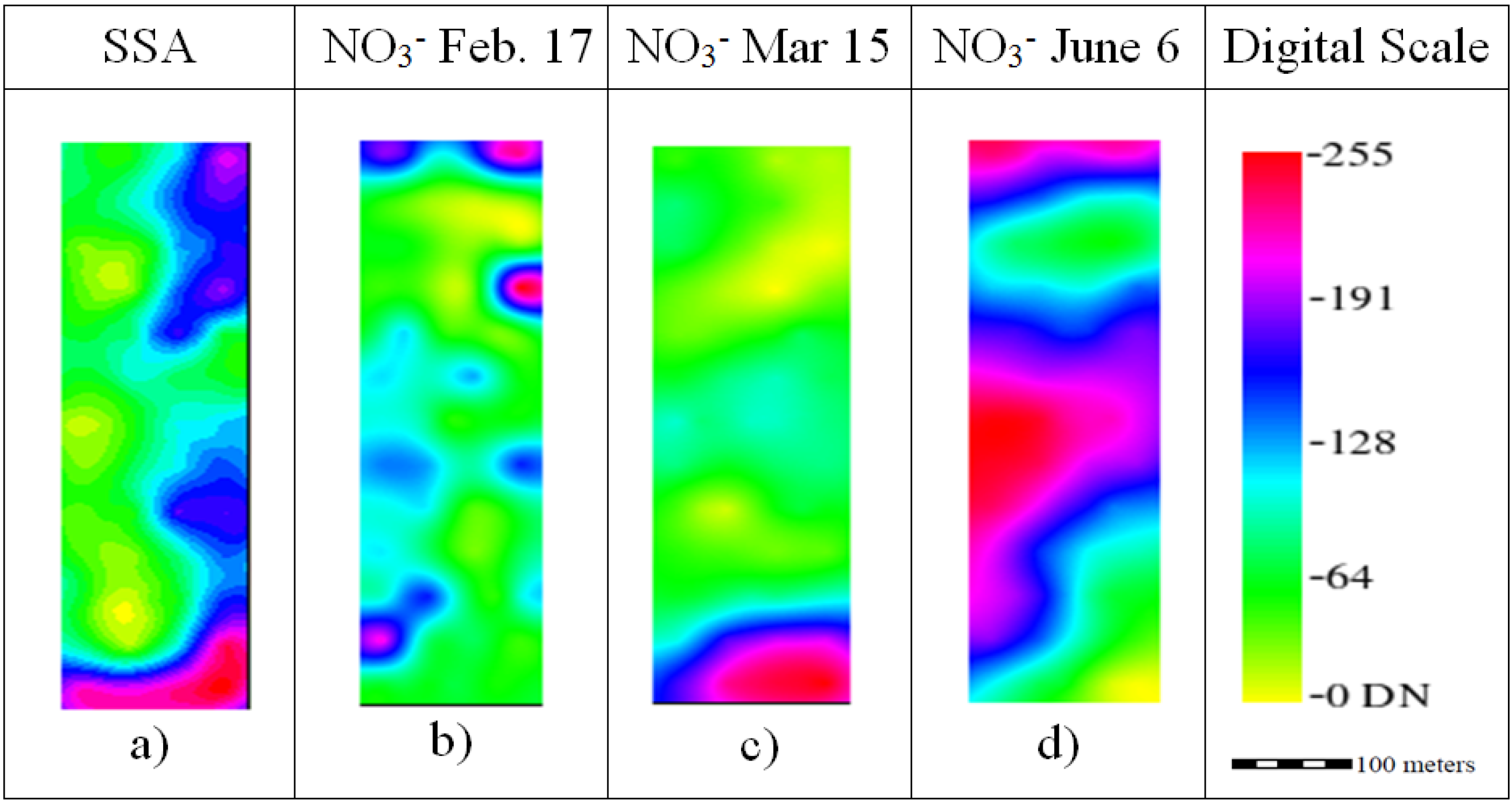
The spatial distribution of the interpolated maps is caused by the behavior of the semivariogram and the interpolation method. The SSA ranged from 73.20 to 95.17 m²/g (Figure 3a) using the average value of 81.29 ± 4.91 m²/g and the general equations from the work of Banin and Amiel [39] for Israeli soils; it was determined that the soil had a 16.65% ± 3.45% clay content, and this corresponds to a bulk density of 1.46 g/cm³ (considering a 55% sand content). The spatial behavior of the nitrate was somehow irregular; this is caused by the ability of this nutrient to move because it is not well adsorbed by the soil particles. Nevertheless, the average nitrate values decreased as the crop developed from 8.24 ± 4.30 ppm in February and 5.42 ± 0.72 ppm in March (Figure 3c) to 4.21 ± 0.21 ppm.

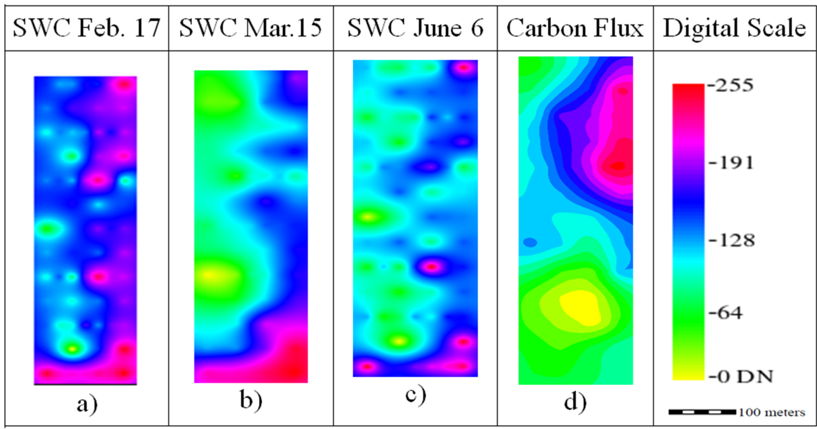
The SWC maps had a similar spatial distribution (Figure 4a–c), with increasing water contents from east to west. The average SWC values decreased from 11.46% ± 0.40% in February (Figure 4a), to 11.20% ± 0.40% in March (Figure 4b) to 3.91% ± 0.37% in June (Figure 4c). The carbon flux had the average measured value of 0.98 ± 0.34 μmol CO₂ m⁻²·s⁻², and the distribution of the carbon flux indicates that the upper right part of the field had more organic matter.

Figure 3. Ordinary kriging raster images rescaled to digital number (DN) range for the production factors Soil Specific Area (SSA) and Nitrate.

Figure 3. Ordinary kriging raster images rescaled to digital number (DN) range for the production factors Soil Specific Area (SSA) and Nitrate.

Figure 4. Ordinary kriging raster images rescaled to digital number (DN) range for the production factors Soil Water Content (SWC) and Carbon flux.

Figure 4. Ordinary kriging raster images rescaled to digital number (DN) range for the production factors Soil Water Content (SWC) and Carbon flux.

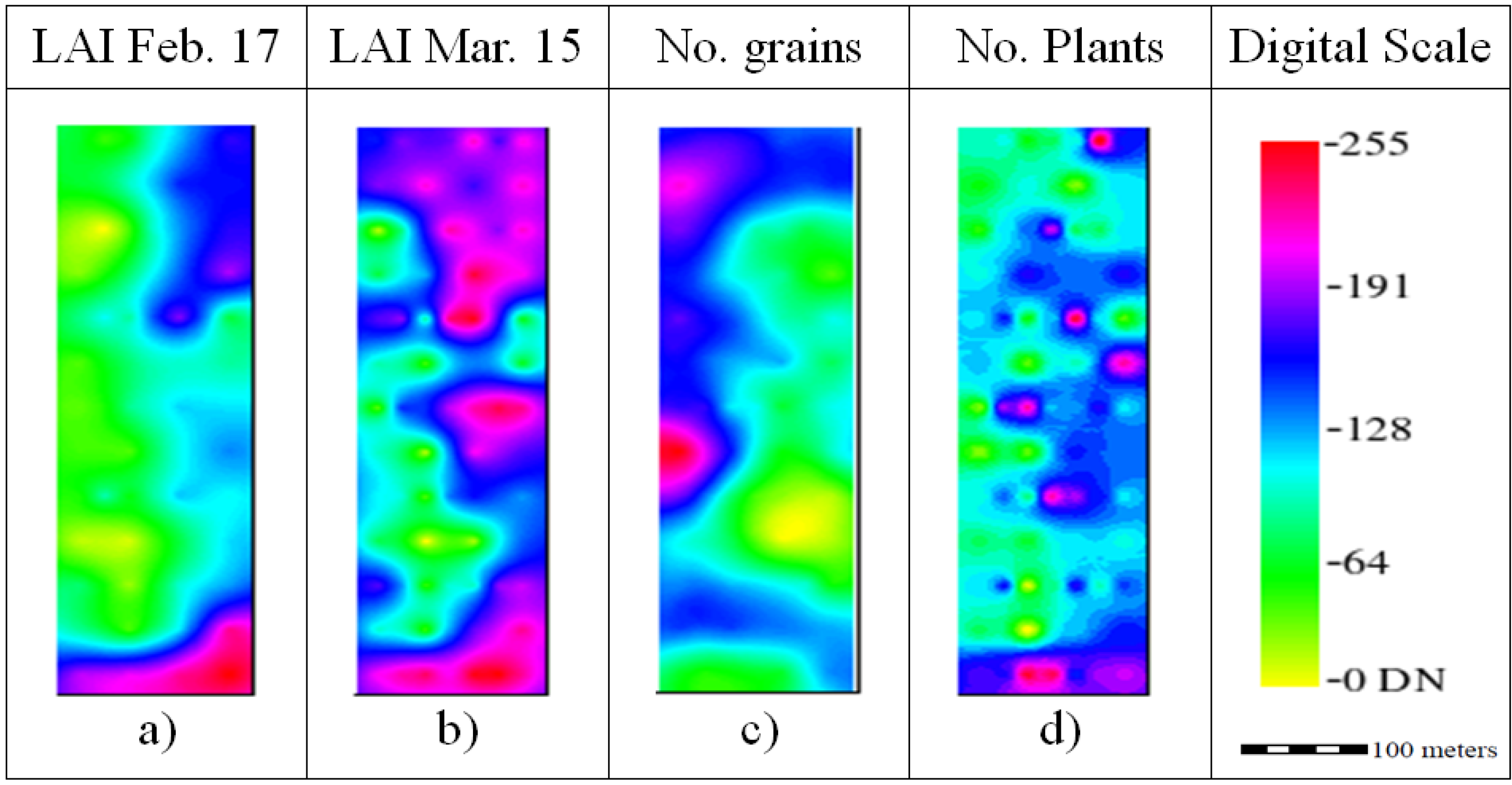
The LAI for February and March (Figure 5a,b) had similarities to SSA and SWC. In fact, the LAI increased from 2.51 ± 0.41 in February (Figure 5a) to 3.56 ± 0.35 in March (Figure 5b) and from east to west. The average number of grains was 3547.3 ± 399.25 n/m² (Figure 5c), and the average number of plants was 503.25 plants/m² (Figure 5d). These two yield parameters seem to be inversely related, with areas of high number of grain density related to low plant density areas.

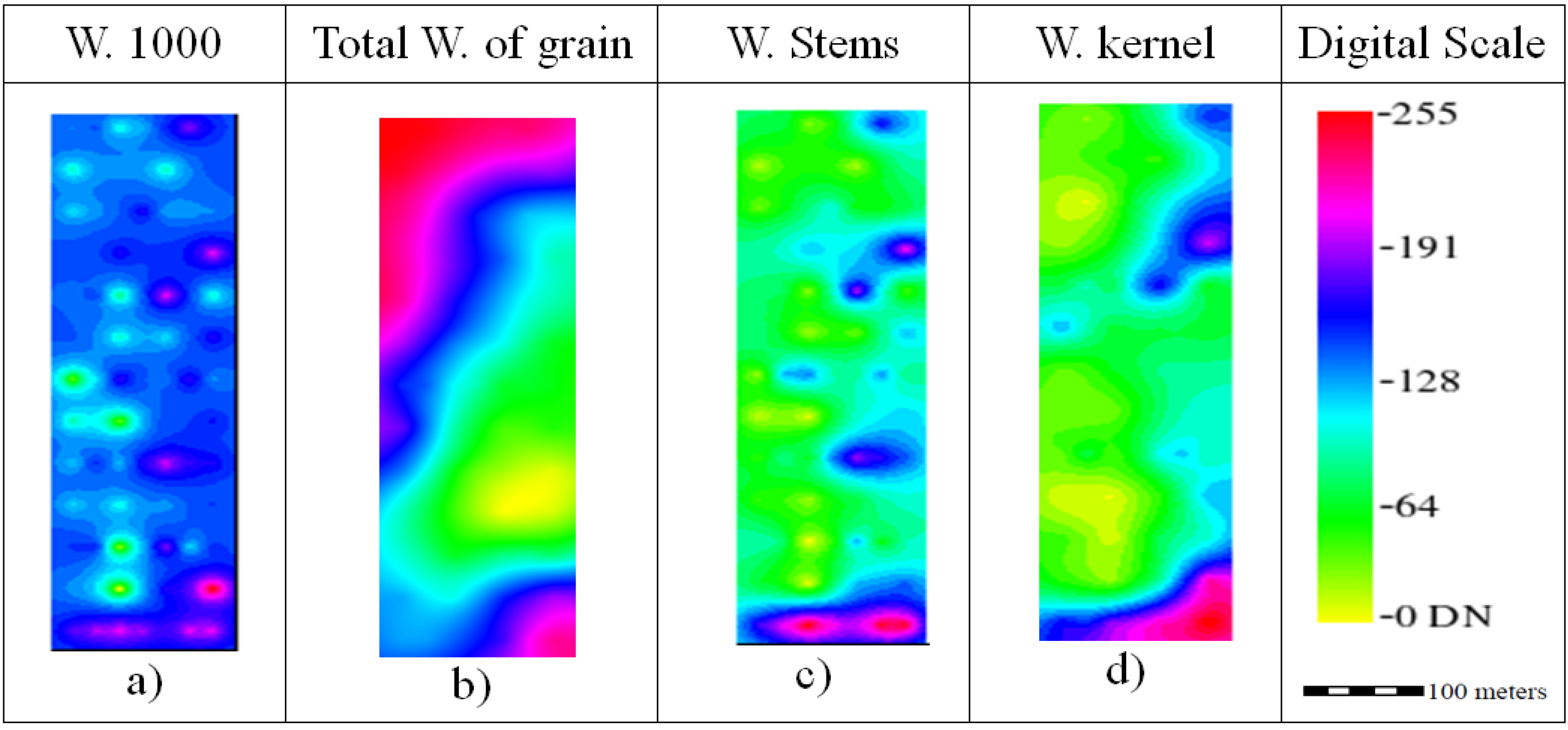
The average weight of 1000 kernels was 37.6 ± 2.75 g (Figure 6a). As indicated by the nugget/sill ratio (Table 1), this trait showed a strong spatial correlation, and the range of the semivariogram is small; the map that was obtained had some “bull eyes”, a feature that is more typical of IDW. The total weight of grain (Figure 6b) is the most important yield parameter because it represents the actual economic production; the average value was 1.88 ± 0.11 t/ha.

The weight of stems (Figure 6c) and kernel (Figure 6d) shared the same behavior because they represent the lower and upper biomass of the plant; the average weight of the stem was 0.93 ± 0.21 t/ha, and the average weight of the kernel was 1.16 ± 0.21 t/ha.

Figure 5. Ordinary kriging raster images rescaled to digital number (DN) range for the yield components Leaf Area Index (LAI), Number of grains and Number of plants.

Figure 5. Ordinary kriging raster images rescaled to digital number (DN) range for the yield components Leaf Area Index (LAI), Number of grains and Number of plants.

Figure 6. Ordinary kriging raster images rescaled to digital number (DN) range for the yield components weight of 1000 grains, weight of stems and weight of kernel.

Figure 6. Ordinary kriging raster images rescaled to digital number (DN) range for the yield components weight of 1000 grains, weight of stems and weight of kernel.

Principal Component Analysis Results

The data show that durum wheat yield is strongly affected by variability in soil parameters (soil water content recorded in 17 February 2004, soil water content recorded in June 6, Nitrate in February 17, CF and, SSA), and thus, the average production can be substantially lower than its potential. However, the objective of this research is to give a mechanistic explanation of the yield variation, something that depends on the conjoint effects of several contrasting or additive factors. PCA results could adequately investigate which main production factors affect yield spatial variation. In this research, it was shown that areas with the lowest biomass production were also those characterized by low carbon flux and high SSA and SWC, parameters that were all significantly related to the yield. Therefore, the use of an appropriate site-specific practice may be expected to substantially increase the average yield. Surprisingly, the effect of nitrate on the crop yield was low because the SWC was a limiting factor.

Correlation coefficients based on kriged maps are presented on Table 2 and Table 3. The correlation coefficient of the PCA from the production factors is given in Table 2. The cumulative results of PC1, PC2, and PC3 account for 85.52% of the data variance. The PC1 explained 48.50% of the data variance, whereas PC2 and PC3 explained 23.53% and 13.48%, respectively. This high cumulative result indicates that these three maps should contain sufficient information to explain internal relations between different producing factors.

Table 2. Correlation coefficient between each production factor and each principal component.

Parameters	PC1	PC2	PC3
Carbon flux	−0.02	0.94	−0.11
Nitrate recorded March 15	−0.65	−0.57	−0.16
Nitrate recorded February 17	0.3	−0.19	−0.74
Nitrate recorded June 6	0.78	−0.07	−0.57
Soil specific area	−0.89	0.23	−0.26
Soil water content recorded March 15	−0.89	−0.13	−0.19
Soil water content recorded February 17	−0.82	0.27	−0.28
Soil water content recorded June 6	−0.81	0.2	−0.28

Table 2. Correlation coefficient between each production factor and each principal component.

Parameters	PC1	PC2	PC3
Carbon flux	−0.02	0.94	−0.11
Nitrate recorded March 15	−0.65	−0.57	−0.16
Nitrate recorded February 17	0.3	−0.19	−0.74
Nitrate recorded June 6	0.78	−0.07	−0.57
Soil specific area	−0.89	0.23	−0.26
Soil water content recorded March 15	−0.89	−0.13	−0.19
Soil water content recorded February 17	−0.82	0.27	−0.28
Soil water content recorded June 6	−0.81	0.2	−0.28

Table 3. Correlation coefficient between each yield factor and each principal component.

Parameters	PC1	PC2	PC3
LAI recorded March 15	−0.78	−0.39	−0.36
LAI recorder February 17	−0.94	−0.17	−0.16
Number of grains	0.55	−0.75	−0.01
Number of plants	−0.78	0.09	0.47
Weight of 1000 grains	−0.8	−0.04	0.34
Weight of kernel	−0.94	−0.14	0.02
Weight of stems	−0.89	0.03	0.38
Total weight of grain	0.10	−0.98	0.11

Table 3. Correlation coefficient between each yield factor and each principal component.

Parameters	PC1	PC2	PC3
LAI recorded March 15	−0.78	−0.39	−0.36
LAI recorder February 17	−0.94	−0.17	−0.16
Number of grains	0.55	−0.75	−0.01
Number of plants	−0.78	0.09	0.47
Weight of 1000 grains	−0.8	−0.04	0.34
Weight of kernel	−0.94	−0.14	0.02
Weight of stems	−0.89	0.03	0.38
Total weight of grain	0.10	−0.98	0.11

The correlation coefficient of PCA for the yield is given in Table 3. The performance of the PCA of the yield was slightly better than the PCA of the production factor because PC1, PC2, and PC3 explained 92.04% of the data’s variability. The PC1 explained 51.52% of the data variance and showed a specific grouping of biological parameters: LAI; number of plants; weight of kernel, stem, and weight of 1000 grains. The major economic yield parameter (total weight of grain) was in PC2 together with the number of grains. The PCA results and the accumulative percentage of explained variance from both production factor and yield were acceptable, and the three PCs from the two groups were sufficient for data analysis of the rasters and their relations.

Factor Loading

Analysis of correlation between the PC and the factors responsible for its creation was used to determine the most important rasters for the creation of each PC. This analysis is called factor loading. By determining which input maps were important for each PC, it was possible to determine the relation between several factors.

SWC and SSA were the parameters that exerted the most influence among all the production factors in PC1. Nitrate had some influence in PC1, but the result was unclear because of different signs and a high correlation of one of the nitrate dates in PC3. The most influencing production factor in PC2 was the carbon flux. All the results for PC3 have a negative value of correlation coefficient; normally, each PC has factors that influence the cloud of points in one direction or another, but in this case, all the factors had a negative correlation, meaning that all push the cloud only in one direction [40].

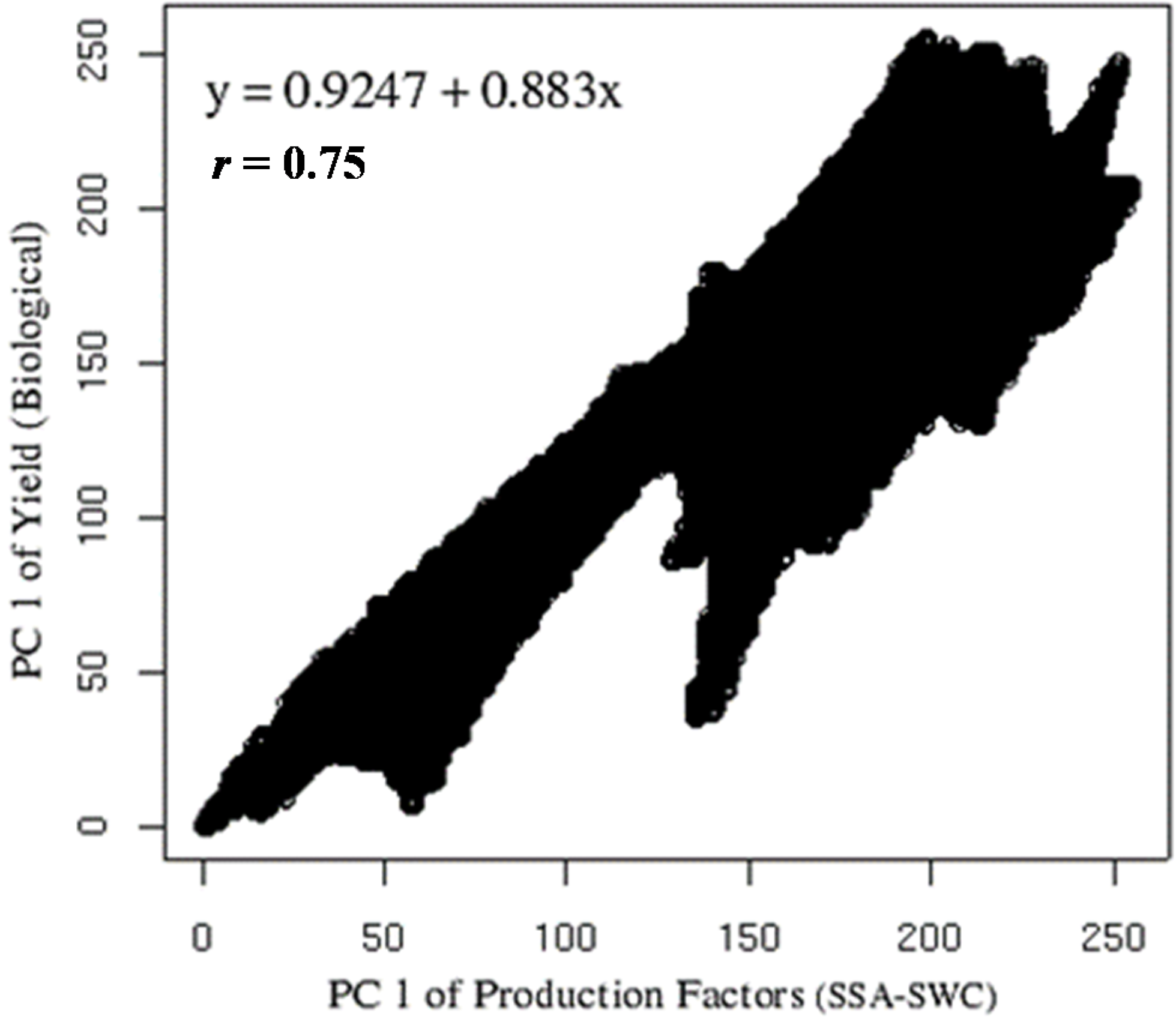
The majority proved that PCA can be used to study the relation between soil properties and that all the different yield factors can be obtained by a correlation between the different PCs of each group. Figure 7 present the correlation between the two rasters, one belonging to the production factor group and the other from yield parameters. It showed a very high coefficient of determination (r = 0.75) with an almost linear behavior (y = 0.9247 + 0.833x). Despite the relation between SSA-SWC with biological yield, this is less important than the relation of economic yield with production factors; therefore there is the need to see how yield parameters are related to SSA-SWC.

Figure 7. Correlation between PC1 of production factors (Soil Specific Area and Soil Water Content) and PC1 of yield components (Leaf Area Index, weight of kernel and stems). Data rescaled to digital number (DN) range of 0–255.

Figure 7. Correlation between PC1 of production factors (Soil Specific Area and Soil Water Content) and PC1 of yield components (Leaf Area Index, weight of kernel and stems). Data rescaled to digital number (DN) range of 0–255.

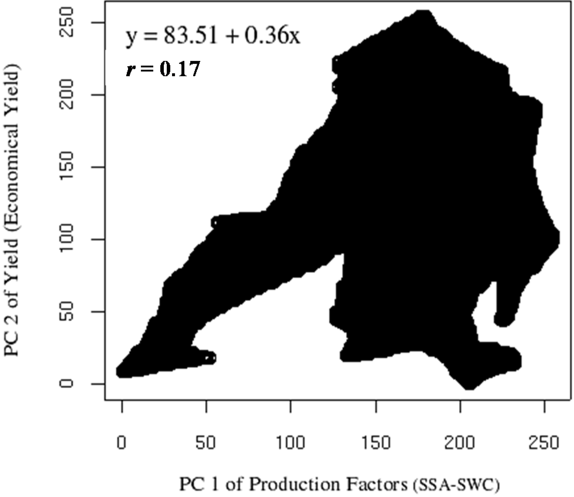
Figure 8 presents the correlation between the PC1 of production factors SSA and SWC and PC2 of yield (total weight and number of grains). This correlation was weak r = 0.17 (y = 83.51 + 0.36x). In the same correlation, it was observed that until the value of 125 DN range, the correlation was high (r = 0.91) and almost linear, but the correlation became null after this value. This change of behavior around the value of 125 DN range also exists on the biological yield correlation, where one part of the cloud starts to divert from the almost perfect linearity. According to Webster and Oliver [41], this behavior may indicate biological saturation response, where above certain threshold, the effect of one or several of the parameters decreases or stop having an impact.

Figure 8. Correlation between PC1 of production factors (Soil Specific Area and Soil Water Content) and PC2 of yield components (total weight and number of grains). Data rescaled to digital number (DN) range of 0–255.

Figure 8. Correlation between PC1 of production factors (Soil Specific Area and Soil Water Content) and PC2 of yield components (total weight and number of grains). Data rescaled to digital number (DN) range of 0–255.

4. Discussion

The use of precision agriculture tools and PCA in plant production factors and yield of an organic field helped reduce the level of complexity between the measured parameters, eliminating data redundancy and resulting in feasible relations. According to Lopez-Granados et al. [42], knowledge on spatial dependence helps to calculate the sampling interval and develop an accurate site-specific application scheme. Therefore, the feasibility of precision farming applications may increase with the degree of spatial dependence.

Data analysis showed a wide variability within the organic field, resulting in inefficient use of resources. Therefore, the use of an appropriate site-specific practice may be expected to substantially increase the average yield [43]. In fact, some parameters change gradually across the field, whereas others show a patchy distribution. The carbon flux, SWC, and nitrate recorded in March were weakly spatially dependent; thus, additional samples at smaller lag-distances may be needed for those parameters. Nonetheless, higher sampling density could be uneconomic.

Instead of having several data rasters, the PCA “compressed” the information in a reliable way, facilitating further analysis. The PCA results showed the relation between multiple parameters as well as which plant production factors were explanatory of the yield results. The carbon flux does not relate to any other parameter; therefore, it had a specific PC. Nitrate had two parameter associated to PC3, but the behavior of nitrate is not clear because it also integrates in part PC1. The most important plant production factor was SWC followed by SSA.

For yield factor, the weight of 1000 grains was grouped in PC1, concluding that when the biomass of the crop increases, the weight per grain also increases. The major economic yield parameter (total weight of grains) in PC2 indicated the distinctive behavior between the biomass and the total grain production. Also, an analysis to the different signs showed that the higher the biomass, the lower was the number of grains and total weight of grain. Therefore, the increase of weight per grain caused by an increase of biomass is not sufficient to increase total production.

The correlation (r) between the biological yield parameters and the PC of SSA-SWC was high, further proving the proper arrangement of plant production factors and yield according to the most important PCs, the influence of SWC-SSA as the major influencing factor for biomass.

The PC1 also showed a different cloud orientation for the group of biological yield, such as total weight and number of grains. This indicates that when LAI and weight of kernel, stem, and weight of 1000 grains are higher, there should be a decrease on the number of grains and total weight of grain (economic yield) and vice versa. This indicates that higher biological biomass will produce less grain, but heavier (because the weight of 1000 grains will be higher), and a lower economic yield. Similar results were found by Dong et al. [44] when wheat cultivars were grown in a dry year and without irrigation.

5. Conclusions

The data show that durum wheat yield is strongly affected by soil parameter variability, and thus, the average production can be substantially lower than its potential. From the Principal component analysis raster images for soil parameters and yield, PC1 explained 48.50% of the data variance. The correlation between the rasters arising from the PC1 of soil and yield parameters showed high linear correlation (r = 0.75). The objective of reducing the number of raster necessary to analyze the reasons behind the specific yield was achieved and still preserving a high percentage of useful information. Soil water content was the limiting factor to grain yield and not nitrate as in other similar studies.

The use of precision agriculture tools and PCA helped reduce the level of complexity between the measured parameters by the grouping of several parameters in the different PC, creating a sort of “compression”, eliminating data redundancy, and resulting in feasible relations. The present research shows that precision agriculture tools can be applied in small organic fields, reducing costs and increasing average wheat yield. Consequently, some site-specific applications could be expected to improve the yield without increasing excessively the cost for farmers and, at the same time, enhance environmental and economic benefits [45]. For example the carbon flux distribution indicates that the upper right part of the field had more organic matter and with this knowledge it can be saved money when applying manure. Also, it can be provided more water in the areas of the field that have lowest soil water content using precision irrigation and by using less manure at the southern part of the field that presented high nitrate in March (Figure 3c).