A Standardized Framework for Cleaning Non-Normal Yield Data from Wheat and Barley Crops, and Validation Using Machine Learning Models for Satellite Imagery

Abstract

Modern combine harvesters can collect real-time geolocated yield data, but it is subject to errors. Various protocols have been proposed to clean this data, each with varying levels of complexity. This data is valuable for precision agriculture to implement site-specific management and to train models to predict yield using remote sensing data. Machine learning and deep learning techniques have shown their potential for precision agriculture, and their performance shows no significant differences between models trained with data cleaned using a computationally demanding protocol or a simpler one, such as parametric filtering. However, parametric filtering approaches primarily rely on statistics that are highly sensitive to data distribution and do not effectively filter inliers. The objective of this study is to develop a data-cleansing method that leverages robust statistical measures, specifically the median and interquartile range, to effectively identify and filter outliers and inliers while retaining valid observations in datasets collected from combine harvesters, thereby minimizing the influence of non-normal data distributions. Different levels of data cleaning were applied to a total of 7399 ha of wheat and barley crops, and the quality of each cleaning level was compared. The selected protocol improved the spatial structure of the data, deleting up to 42% and 33% of the data at the polygon level, for wheat and barley, respectively. It increased the mean and median, and decreased the standard deviation and coefficient of variation of the data. Between 78.7% and 82.9% of the fields showed a normal distribution after applying the selected method, and machine learning performance improved compared with the raw data. Compared with previous data cleaning studies, the present work proposes an automatic, low-computational, parametric filtering method that uses robust statistics for non-normal distributions. In addition, its scalability has been demonstrated by applying the method to a large dataset, improving data quality and the performance of yield-prediction ML models in all cases.

1. Introduction

As the world population is expected to reach 10.3 billion by the mid-2080 [1], increasing food production is essential to meet the food requirements of this rapidly growing society. Until now, the increase in final production has been achieved thanks to the combination of variety breeding, an increase in cultivation area, and the great use of inputs. However, since many crops are nearing their maximum physiological yield [2], the negative effects of excessive fertilizer application are undeniable in the environment [3], and natural resources are increasingly limited.

In view of these limitations, precision agriculture (PA) has been presented in the last few decades as a solution that allows site-specific crop management (SSCM) [4] to improve productive potential and efficiency of farm inputs [5].

Within PA, some of the most important sources of information are yield maps and their precise location data, provided by yield monitors installed in combine harvesters and their Global Positioning Systems (GPS) [6]. Using these data for SSCM and the creation of yield prediction models. Nevertheless, even as more growers adopt these technologies, these data are often underused by growers and the industry [7], mainly because of existing anomalies that could jeopardize future decisions based on these data. These errors can be classified into four groups [8]: harvest dynamics (lag time, filling and emptying time), measurement errors related to yield and moisture observations, positioning system accuracy, and harvester operator (speed, harvest turns, and headlands).

In this regard, several authors have highlighted the need to detect and filter these errors prior to any subsequent data analysis. Numerous methodologies have been proposed, most of which have been tested in only a limited number of fields and production areas. Overall, two main approaches are commonly employed:

• Global filtering, in which outliers are removed from the dataset [9]. In the literature, global filtering comprises several types of filters, including the use of complementary harvest data (e.g., moisture measurements, harvester speed, or harvesting pass), biological limits of the crop, and parametric filtering criteria.
• Local, post-processing filtering, where a neighborhood of observations is defined, and inliers are subsequently removed [4,6,8,10]. Local filtering can be performed through different approaches, such as the application of the Local Moran’s spatial correlation index (LM) [6,11], clustering algorithms [7,12], or expert-based manual filtering [13].

In both cases, interpolation techniques such as the Block Kriging and Inverse Distance Weighting (IDW) methods are commonly used to replace the removed data points.

Nevertheless, data-cleaning protocols that rely on complementary harvest information are limited by the fact that such ancillary data are not always available [14]. Similarly, parametric filters based on statistical descriptors such as the mean and standard deviation may be unsuitable for large, multi-location datasets with a large number of fields, as the proportion of fields with non-normal distributions tends to increase. Conversely, local filtering techniques are typically characterized by high computational demands, which do not necessarily yield superior performance when the cleaned data are subsequently used to train ML models [15], and many of these approaches lack full automation.

In this sense, researchers in other domains have recommended data transformations, such as the logarithmic transformation, the min-max method, or z-score normalization [16], to obtain a dataset with a normal distribution. Even so, these techniques are not helpful for all datasets and may be difficult to interpret in agriculture. Another feasible option is to use other parameters that are more reliable in non-normal distributions for the filtering process, such as the median or the interquartile range (IQR) [17].

For this purpose, in this paper, the non-normality of raw yield datasets is tested and validated for a large dataset, including two different crops (wheat and barley), five locations, and four different growing seasons. Once this statement is verified, the paper aims to select a new data-cleaning protocol that can be easily automated with low computational expense. This study proposes global and local filtering, using the median and interquartile range as robust statistics to clean skewed data, along with different combinations of coefficient limits. The selection of the optimized data cleaning method is based on an analysis of the data’s internal structure and on enhancing the performance of the machine learning model trained on Sentinel-2 reflectance data and filtered yield data. The proposed method is applied in 7399 ha of wheat and barley.

2. Materials and Methods

2.1. Site of Study

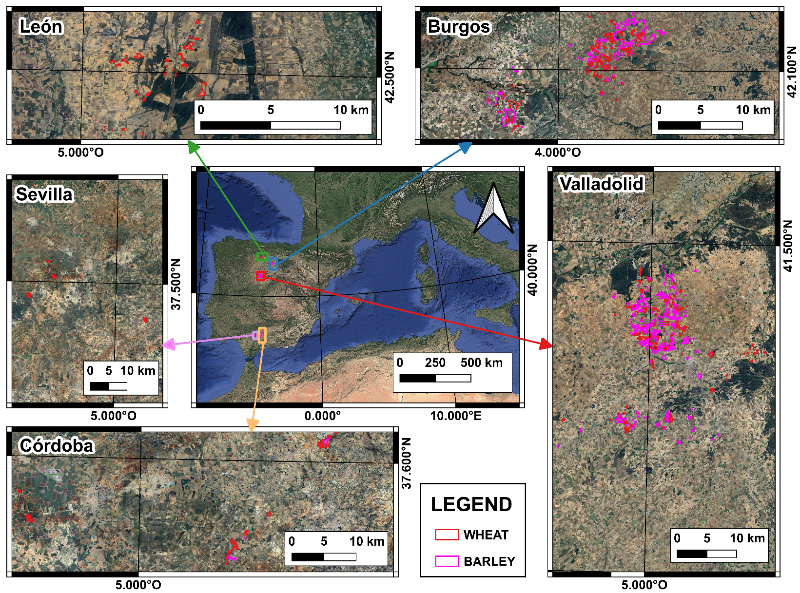
The study was conducted using yield data from five of the main wheat and barley production areas in Spain (Figure 1): Burgos, Córdoba, León, Sevilla, and Valladolid. A total surface of 7399 ha of yield data was used in the data cleaning study (3178 ha and 4221 ha for wheat and barley, respectively), distributed in 648 fields (309 and 339 fields for wheat and barley, respectively) over 4 crop seasons (from 2020 to 2023). On the side of wheat, data from the 5 different locations were available, while in barley, only three locations had available yield data (Burgos, Córdoba, and Valladolid). The available yield data corresponds to winter wheat and barley crops, which were sown in November. The crop management of wheat and barley fields in Spain follows the recommendation of López-Bellido et al. [18,19].

According to the Köppen Climate Classification (KCC), the studied areas have different characteristic climates. Therefore, the climate for each location is: Temperate oceanic climate (Cfb) for Burgos, Semiarid climate (BSh) for Córdoba, warm-summer Mediterranean climate (Csb) for León, hot-summer Mediterranean climate (Csa) for Sevilla, and arid steppes (BSk) for Valladolid. The soil type for these areas is calcimorphic, except for the León area, which presents an umbrisol soil type [20].

2.2. Satellite Data

The satellite data were obtained from a Multi-Spectral Instrument (MSI) on board two twin satellites (Sentinel-2A and Sentinel-2B) that fly in the same orbit but are phased 180°, allowing the acquisition of wide-swath, high-resolution images with a 5-day time frequency [21]. The optical instrument sampled 13 spectral bands, 10 of which were used (

Table 1. Characteristics of the Sentinel-2 used bands.

Sentinel-2 Band	Central Wavelength (nm)	Spatial Resolution (m)
B02-Blue	450	10
B03-Green	560	10
B04-Red	665	10
B05-Vegetation Red-Edge	705	20
B06-Vegetation Red-Edge	740	20
B07-Vegetation Red-Edge	783	20
B08-NIR	842	10
B8A-Narrow NIR	865	20
B11-SWIR	1610	20
B12-SWIR	2190	20

). Only cloud-free images were used, downloaded from ESA’s official Copernicus Browser platform. The downloaded images were level 2A products that provide Bottom-of-Atmosphere (BOA) reflectance data.

2.3. Yield Data Acquisition

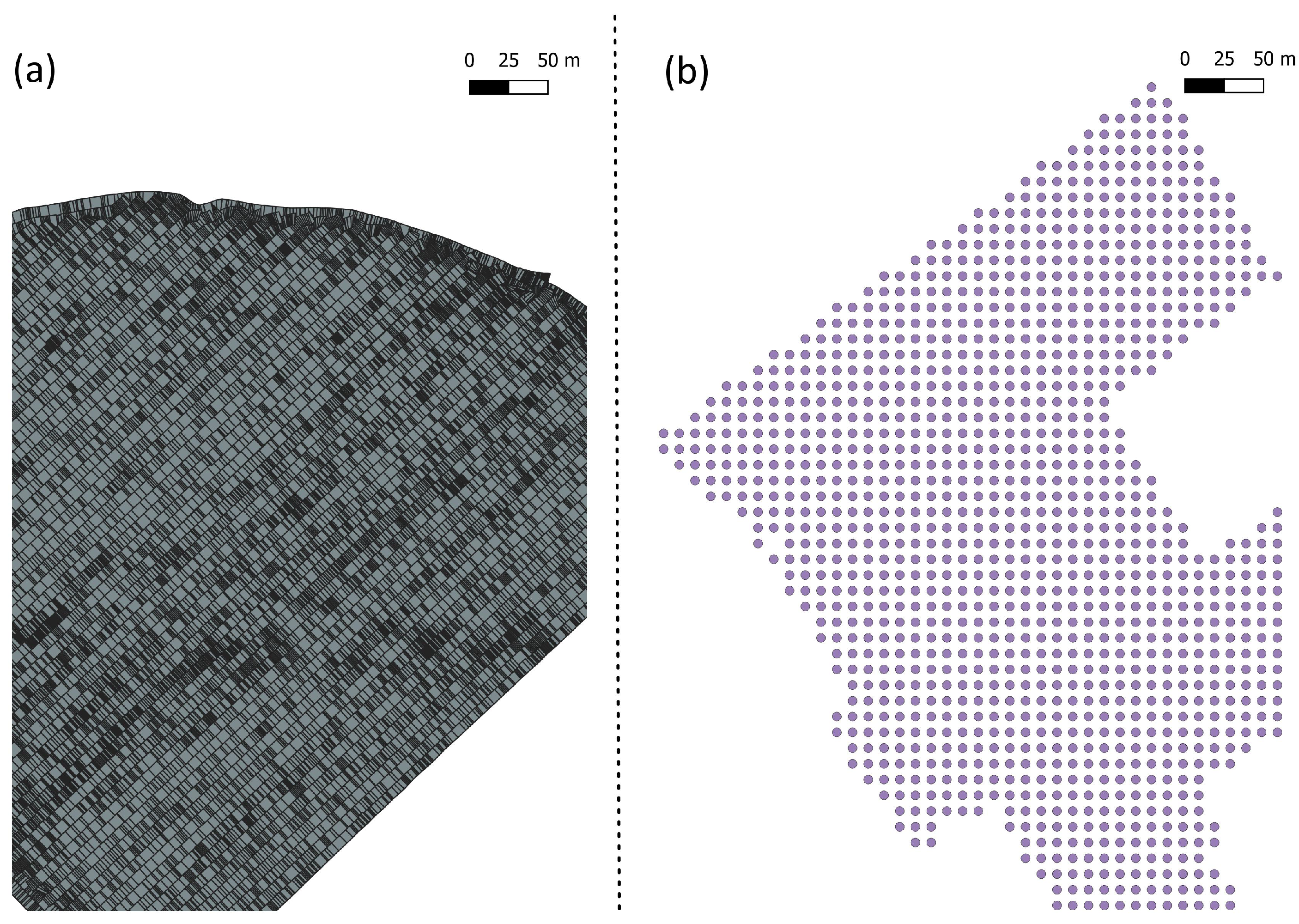
The crops’ final yield data was recorded using two different Yield Track software, one installed by TOPCON Corporation (Tokyo, Japan) and the other by Trimble company (Westminster, CO, USA). A total of three combine harvesters were used for data acquisition. Both companies’ measurement systems are based on volumetric grain flow estimates from optical sensors before the grain enters the combine harvester hopper. The software that generates yield maps includes internal calibration based on the crop type, so combine operators select the grain type to be harvested and calibrate the sensors before starting. However, the representation of the data in the resulting shapefiles differs. TOPCON (Yieldtrakk YM-1) (Topcon Positioning Systems, Inc., Livermore, CA, USA) creates a layer composed of polygons with an irregular surface and a constant width that matches the cutting width (7.5 m for wheat and barley crops) of the combine (Figure 2a), whereas Trimble (Trimble Ag) (Trimble Inc., Westminster, CO, USA) creates a layer of points (Figure 2b). The yield maps of Córdoba, León, Sevilla, and Valladolid were created using TOPCON software, while the Burgos yield maps used Trimble software. TOPCON yield maps were downloaded directly from the combine harvester, while the Trimble yield maps were obtained from the company. These datasets were already preprocessed and free of yield values outside the biological limits of the crops.

2.4. Study of Data and Data Processing

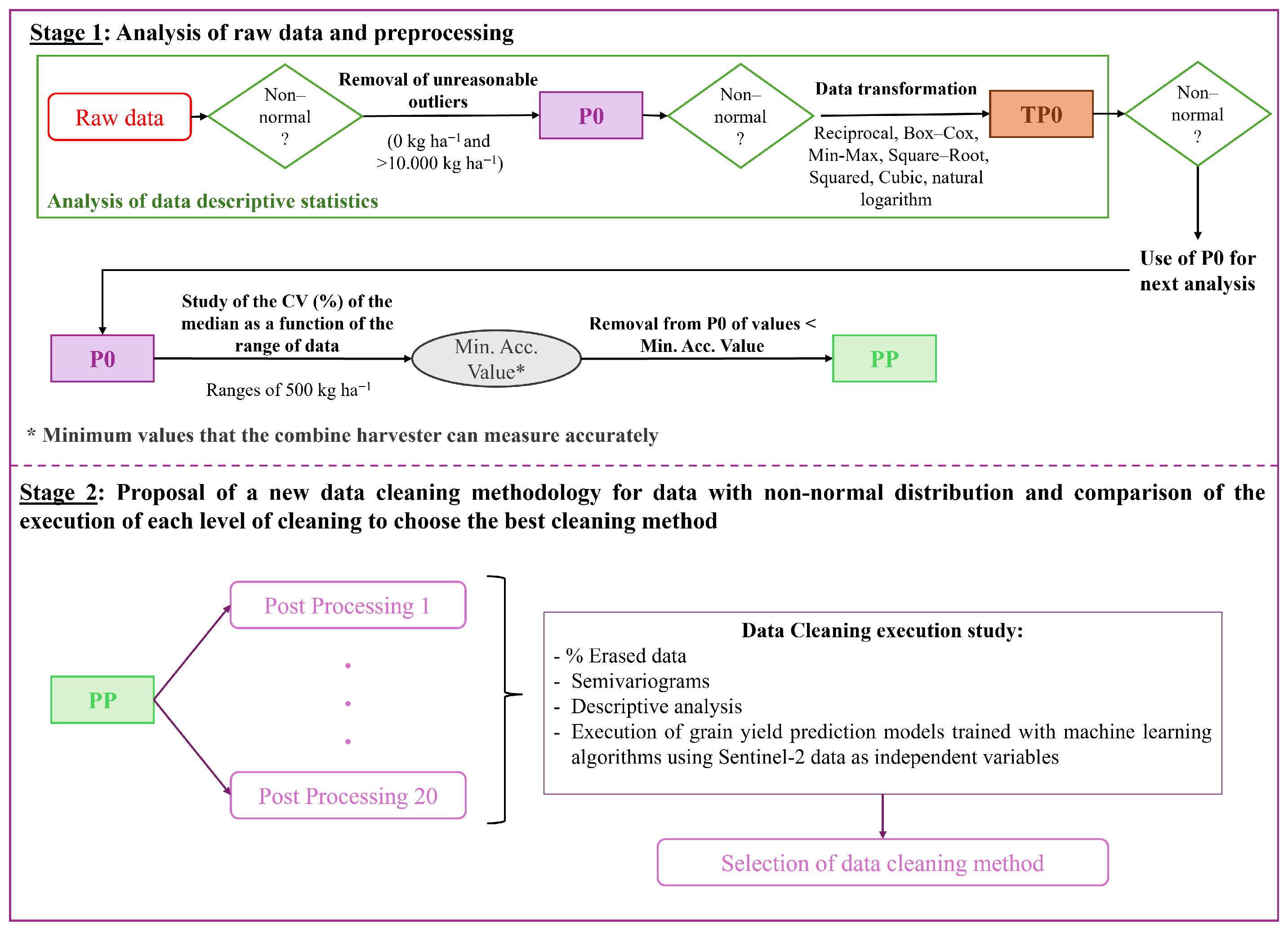
Figure 3 shows the following workflow for the data cleaning study. It’s composed of two stages. Stage 1 defines the starting point for the analysis by filtering the raw performance data at P0 (biological limits), evaluating the distribution/transformations, determining the minimum precision threshold value, and providing a preprocessed database (PP). Stage 2 cleans the PP data (Figure 4), using 4 global combinations (G1.0–G2.5) and 16 final combinations (G × L). The optimal cleaning level is selected by comparing the performance maps obtained with the statistical indicators described in Section 3 (percentage of data removed, dispersion, normality metrics, and spatial distribution).

2.4.1. Analysis of Raw Data and Preprocessing

A descriptive analysis of the data was carried out in the original (raw) and preprocessed (P0) data. The P0 datasets were obtained by deleting from the raw data the measured values outside the biological limits of wheat and barley crops (0–10,000 kg ha⁻¹). The selected statistics for the descriptive analysis were the minimum (Min) and maximum (Max) values, the Mean, the median, the coefficient of variation (CV), the Fisher-Pearson coefficient of skewness (Skew), and Pearson’s coefficient of kurtosis (Kurt). In this study, normality was examined using asymmetry and kurtosis thresholds in accordance with descriptive statistical criteria. Subsequently, the percentage of fields that presented a normal distribution of yield data was calculated for each location and crop. The dataset was considered normally distributed when its skew was within the range of −0.5 to 0.5, and its kurtosis was within the range of −2.0 to 2.0.

Once the normality of the P0 data is tested, several methods of data transformation [17,22,23] are applied to determine is the percentage of the field that presents a normal distribution increases with respect to P0, and transformed data should be used for the next analysis step; otherwise, P0 data will be used. The selected transformations were 7, chosen after reviewing the existing literature: Reciprocal (${\displaystyle \frac{1}{x_i}}$), Box-Cox, Min-Max, Square Root ($\sqrt{x_i}$), Squared ($x_i^2$), Cubic ($x_i^3$), and common logarithm (log₁₀(x_i)). Afterward, to determine the minimum value that the combine harvester can measure with accuracy (Min. Acc. Value), the data is segmented into groups in function of the yield range (ranges of 500 kg ha⁻¹), and the study of a robust coefficient of variation (CV_median) based on the median and the Median Absolute Deviation (MAD) is made. CV_median values were obtained for each crop, and the two monitoring systems were calibrated on each harvester following the instructions of [10]. The minimum threshold value was considered using a conservative criterion to standardize the methodology across all groups. The decision to use CV_median (Equation (1), where X = $\{x_1,x_2,\dots ,x_i\}$ being $i=1,\dots ,N$) instead of the CV of the mean was made due to the tendency to non-normal distribution that not-cleaned yield data presents, widely presented by other authors [7,24], and this CV analog is more robust to outliers when relative dispersion needs to be measured. Once the range CV_median is calculated, excessively high values in the low ranges of yield, compared to the adjacent ranges, were selected as a sign of low accuracy of the combine harvester. Those value ranges highlighted as low-accuracy were deleted, yielding the PP data, which will be used as base data for applying the data cleaning protocols (stage 2).

$${\mathrm{CV}}_{median}={\displaystyle \frac{\mathrm{MAD}}{\mathrm{Median}}}\times 100={\displaystyle \frac{\mathrm{Median}\left(\right|x_i-\mathrm{Median}\left(\mathrm{X}\right)\left|\right)}{\mathrm{Median}\left(\mathrm{X}\right)}}\times 100$$

(1)

where $C{V}_{\mathrm{median}}$ represents the coefficient of variation based on the median; MAD denotes the median absolute deviation, computed as the median of $|x_i-\mathrm{Median}\left(\mathrm{X}\right)|$, where $x_i$ corresponds to each observation and $\mathrm{Median}\left(\mathrm{X}\right)$ is the median of the dataset. The absolute value operator $|·|$ measures the deviation from the median, and the factor $\times 100$ converts the resulting ratio into a percentage.

Given the unusually high dispersion of data in the lower-yield range, the threshold of 500 kg ha⁻¹ is used as a criterion for data quality rather than as a general physiological bias of the plant. Low yield values may be due not only to crop management anomalies but also to grain flow within the harvester system itself. Consequently, these values are considered to have little validity for processing and modeling.

2.4.2. Proposal of Data Cleaning Methodology and Execution Comparison with Other Data Cleaning Methods

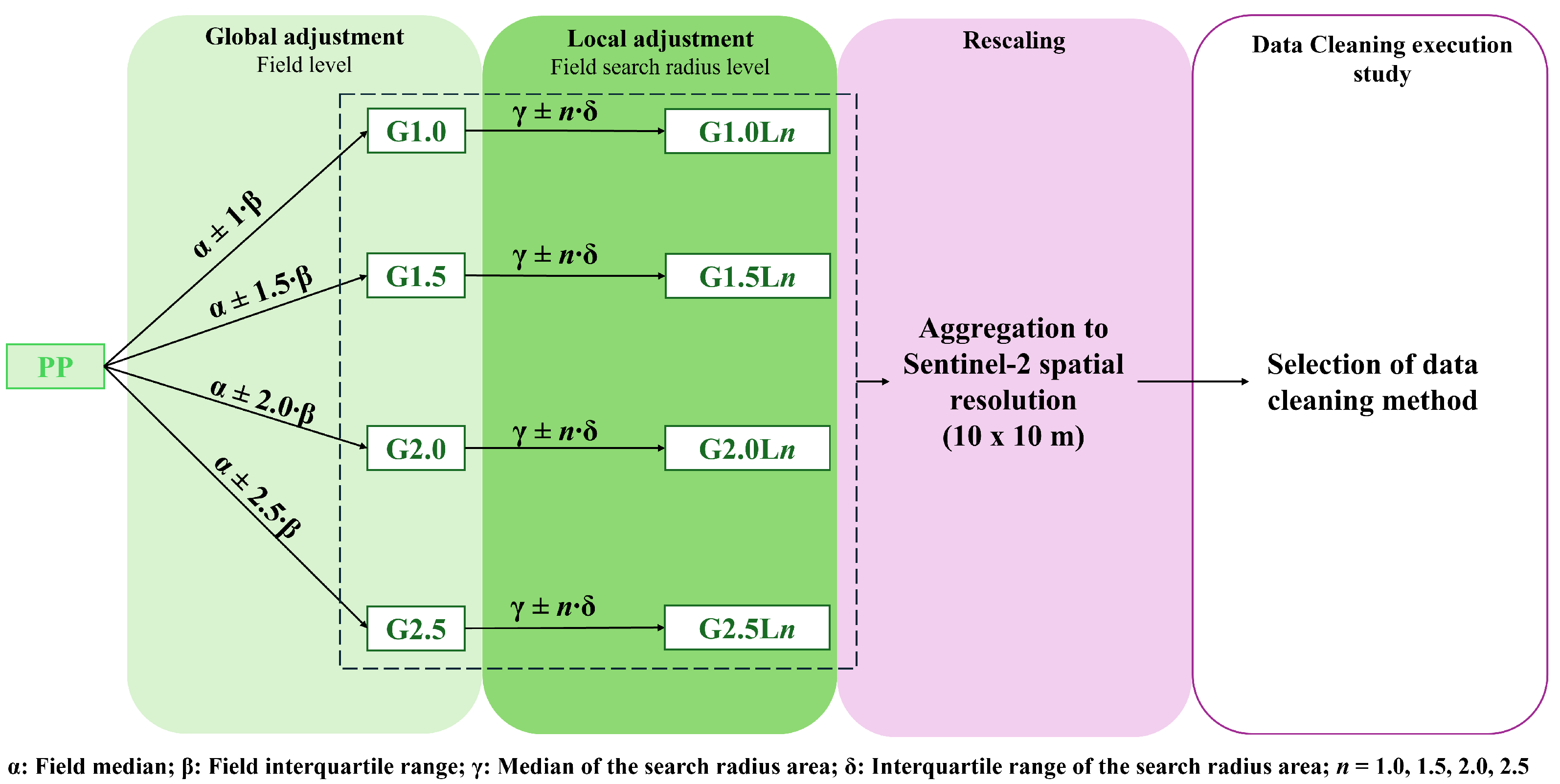
The proposed data-cleaning methodology was introduced with two key objectives: ensuring applicability across all yield datasets and minimizing computational cost. Figure 4 illustrates the proposed approach in detail. For the proposed method to be applied to all yield datasets, the only truth data required for the cleaning process are the yield maps generated by the Yield Track system, as other measurements, such as harvesting speed and grain moisture, may not always be available [14]. The PP level of data obtained at stage 1 was subjected to three levels of processing (global adjustment, local adjustment, and rescaling) before obtaining the final product, which will be used for PA purposes.

1.

Global adjustment: A parametric filtering was carried out at the field level to delete the remaining outliers. It’s based on delimiting a range of yield values for the field and deleting the data points that fall outside the predefined bounds. The upper and lower limits of the range were established using Equations (2) and (3). Four types of global filtering were tested (G1.0–G2.5) based on the coefficient limit (n). The selected n values were 1.0, 1.5, 2.0, and 2.5.

$$\mathrm{Upper}\mathrm{limit}=\alpha +n·\beta$$

(2)

$$\mathrm{Lower}\mathrm{limit}=\alpha -n·\beta$$

(3)

where $\alpha$ denotes the field median; $\beta$ represents the field interquartile range. The parameter n takes the values $1.0,1.5,2.0,$ and $2.5$.

2.

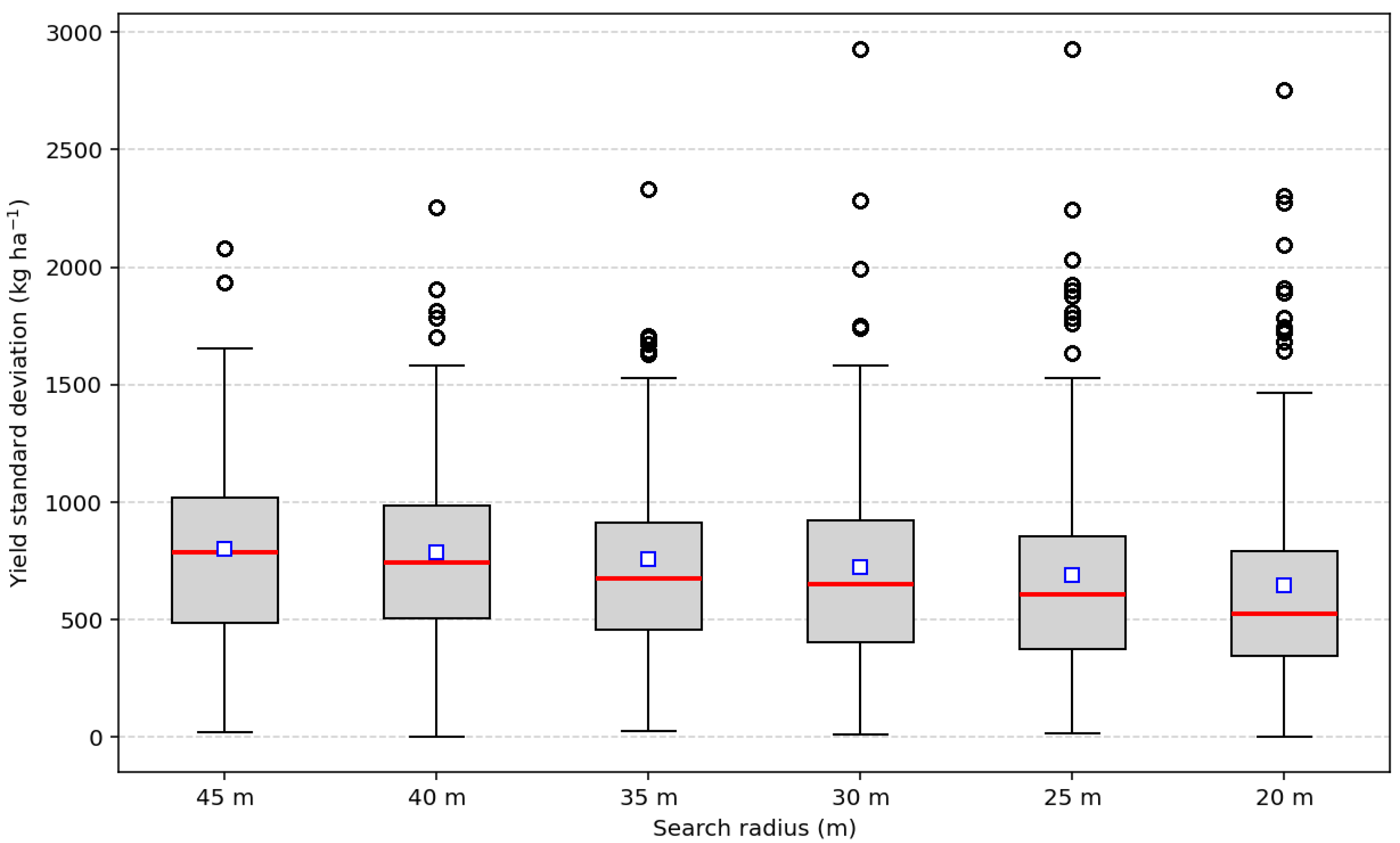
Local adjustment: Once the global adjustment was made, another parametric filtering was carried out within each field to delete the remaining inliers. For this second filtering, a search radius of 40 m [6,10] was used to create distinct neighborhoods within each field. The search radius was set to neighborhoods populated with data from each direction of the combine harvester, with at least one repetition, including 5 harvester passes for TOPCON data and 4 for Trimble data. To verify that the selected search radius was not over-smoothing the data, an analysis of the standard deviation of yield in function of different search radius was made (Figure 5). As the search radius increases, the SD mean approaches the median, and the percentage of anomalous data and the CV decrease, indicating that smaller radii are more strongly influenced by noise. Nevertheless, between 40 and 45 m search radius, the improvement is minimal, indicating that increasing the search radius more than 40 m will be over-smoothing data. Upper (Equation (4)) and lower (Equation (5)) limits were established for each neighborhood, and data points that fell outside the bounds were deleted. For each resulting map of the tested global filtering, four types of local filtering (L1.0–L2.5) were tested, depending on the used n. The selected n values were 1.0, 1.5, 2.0, and 2.5.

$$\mathrm{Upper}\mathrm{limit}=\gamma +n·\delta$$

(4)

$$\mathrm{Lower}\mathrm{limit}=\gamma -n·\delta$$

(5)

where $\gamma$ corresponds to the median within the search-radius area; and $\delta$ denotes the interquartile range of the search-radius area. The parameter n takes the values $1.0,1.5,2.0,$ and $2.5$.

3.

Rescaling: All the maps resulting from global filtering (4 levels), and global+local filtering (16 levels) were rescaled into a 10 × 10 m grid, corresponding to Sentinel-2 higher spatial resolution. The 10 m grid is projected in EPSG:32630-WGS 84/UTM zone 30N and explicitly aligned to the Sentinel–2 grid, ensuring that pixel boundaries coincide exactly with the Sentinel–2 10 m bands to prevent spatial shifts. The 10 m gridding was performed by aggregating polygon values using an area-weighted mean based on their spatial overlap with each pixel, while a simple mean of the multiple points falling within the same pixel was made to obtain the pixel yield value.

A parametric filtering procedure was proposed for both global and local filters to obtain a data-cleaning protocol that can be easily industrialized at low computational cost. An automatic cleaning procedure is necessary because it allows use across different contexts without resorting to empirical knowledge. In the literature, parametric global filters have been widely used, but most of the cleaning protocols used mean and standard deviation as filtering statistics [4,6,8,10]. However, these statistics are heavily influenced by data distribution and can lead to an increase in deleted data, erasing data that may not be outliers. Therefore, the proposed protocol relies on statistics that are less sensitive to data distribution, such as the median and the IQR [15,24]. The selection of n values was made based on the existing literature; the most commonly used n values are 3 and 2.5, in accordance with the three-sigma rule. Although the yield monitor data tend to be skewed by harvesting artifacts, the reduction of n to 1.5 has also been applied [4]. Consequently, the value of 3 was omitted, and it was decided to test n values from 1.0 to 2.5 to determine which n combination improved the final data quality the most. The decision to use a parametric local filter rather than other local filtering techniques, such as applying clustering algorithms to detect anomalous data points within established neighborhoods, is justified on the basis of the computational expense. Clean yield data is used as ground truth information for training models that allow PA. Those models are being created using ML and deep learning (DL) algorithms, which are characterized by being less sensitive to anomalous data. In this sense, it has been observed that data cleaned with parametric and more complex filters show similar performance when used to train yield prediction models [15], thus the use of filters with lower computational expense is preferable.

Once the data were cleaned, the proposed levels were compared with the raw and PP data to determine which cleaning level performed better. The comparison began with the study of the percentage of deleted data at the polygon and pixel levels. This was followed by the construction of semivariograms to examine how the different cleaning levels affected the spatial structure of the datasets. A descriptive analysis was also performed, studying the changes in mean, median, SD, CV, Skew, Kurt, and the percentage of fields that present a normal distribution of yield, since raw yield maps often exhibit skewness due to systematic harvester errors or human mistakes, and proper data cleaning allows the distribution of yield data to more closely resemble a normal distribution [25]. Finally, the data was used in conjunction with Sentinel-2 data to train the final yield prediction models, comparing the impact of the level of cleaning on the models’ performance. To train the prediction models, two ML algorithms were used, specifically, PLSR and XGBoost. The employed hyperparameters for PLSR training were 30 components and no variable scaling. In the case of XGBoost, the hyperparameters were 50 trees, a maximum tree depth of 3, a learning rate of 0.05, and a random seed of 0. An independent model was trained for each level of cleaning, location, year, and crop. Each independent dataset was split randomly using a ratio of 80–20%. All models were cross-validated using the test dataset, which was not used during training, using the hold-out validation method. The performance of the models was evaluated using R², the Mean Absolute Error (MAE), and the Root Mean Squared Error (RMSE).

Finally, the selected cleaning level will be compared with the most used data filtering method in the bibliography. Specifically, the 3SD method will be applied, which consists of a global filtering that deletes all the yield measurements that fall outside of the threshold of ${\mathrm{mean}}_{\mathrm{field}}\pm 3·{\mathrm{SD}}_{\mathrm{field}}$ [6,8,13,25,26].

2.5. Software

The processing of yield maps, nitrogen maps, and Sentinel-2 data was carried out using QGIS 3.34.6. Descriptive data analysis and semivariogram computation were performed with the scikit-gstat 1.0.19 and pykrige 1.7.2 libraries. The PLSR models were trained and tested, and model performance metrics were calculated using scikit-learn 1.2.2. The training and testing of the XGBoost algorithm were performed with the xgboost 3.0.5 library. A summary of the software used is provided in

Table 2. Software and libraries used in the study.

Software/Library	Version	Developer/Organization	Official URL
QGIS	3.34.6	QGIS Development Team	https://qgis.org                   (accessed on 12 January 2025)
scikit-gstat	1.0.19	M. Mälicke & contributors	https://scikit-gstat.readthedocs.io (accessed on 25 April 2025)
pykrige	1.7.2	PyKrige Developers	https://pykrige.readthedocs.io (accessed on 30 April 2025)
scikit-learn	1.2.2	scikit-learn Developers	https://scikit-learn.org             (accessed on 31 August 2025)
xgboost	3.0.5	XGBoost Developers	https://xgboost.readthedocs.io (accessed on 1 September 2025)

.

3. Results

3.1. Study of the Data

3.1.1. Raw and Preprocessed Data

A descriptive analysis of the raw and P0 yield data was carried out to determine whether it followed a normal distribution (

Table A1. Yield descriptive statistics of original (Raw) and preprocessed (P0) data of wheat crops. Being n the number of data, Min the minimum value, Max the maximum value, Mdn the median value.

Loc.	Year	Type	n	Min	Max	Mean	Mdn	CV	Skew	Kurt
				kg ha−1				%
BUR	2021	P0	15,255	3	9988	4170	4362	34.9	−0.2	0.3
	2022	P0	13,181	2	9810	2580	2537	37.4	0.9	3.5
COR	2020	Raw	22,570	0	37,770	5056	5483	43.8	0.7	12.9
		P0	21,773	1	10,000	5128	5516	35.9	−0.7	0.2
	2021	Raw	109,299	0	32,284	3453	3579	41.6	0.6	10.9
		P0	106,812	1	9838	3511	3605	37.0	−0.1	0.6
	2022	Raw	22,699	0	32,960	3755	3899	44.9	1.7	26.9
		P0	22,065	1	9734	3820	3933	37.2	−0.4	0.4
	2023	Raw	230,611	0	385,276	1621	805	399.6	25.8	1001.2
		P0	217,274	1	9992	1189	829	98.2	2.8	11.5
LEO	2023	Raw	79,893	0	4,461,868	10,134	2795	424.1	22.1	1547.6
		P0	60,265	1	9994	3278	2798	47.4	1.9	3.9
SEV	2020	Raw	5722	0	50,593	3483	3935	51.1	4.5	107.2
		P0	5523	1	9926	3547	3952	38.6	−0.9	1.5
	2021	Raw	58,847	0	43,886	2053	2064	47.4	3.2	81.4
		P0	56,610	1	9938	2099	2086	40.2	0.8	5.0
VALL	2020	Raw	161,369	0	57,030	4331	4026	60.4	0.8	5.6
		P0	157,237	1	10,000	4360	4066	56.5	0.3	−0.9
	2021	Raw	48,900	0	399,669	3464	3298	186.1	41.1	2253.6
		P0	44,992	1	9941	3392	3416	55.2	0.1	−0.7
	2022	Raw	297,140	0	783,500	1696	1373	221.8	84.2	13,859.8
		P0	279,970	1	9911	1640	1432	66.2	1.5	4.6
	2023	Raw	344,669	0	295,365	1555	1171	221.6	35.0	1763.3
		P0	314,039	1	9997	1548	1270	77.0	1.2	2.1

and

Table A2. Yield descriptive statistics of original (Raw) and preprocessed (P0) data of barley crops. Being n the number of data, Min the minimum value, Max the maximum value, Mdn the median value.

Loc.	Year	Type	n	Min	Max	Mean	Mdn	CV	Skew	Kurt
				kg ha−1				%
BUR	2021	P0	13,612	8	9980	3936	3899	34.4	0.0	0.5
	2022	P0	15,292	1	9616	2666	2540	36.7	1.3	4.6
COR	2021	Raw	17,711	0	26,992	3154	2698	54.8	1.0	5.4
		P0	17,290	1	9890	3217	2737	50.7	0.6	−0.2
	2022	Raw	2540	0	10,657	2232	2440	50.7	0.5	4.1
		P0	2404	1	8231	2346	2494	42.2	0.3	2.2
	2023	Raw	95,048	0	539,489	1912	1267	362.9	38.4	1973.9
		P0	89,612	1	9816	1650	1352	85.1	1.2	2.0
VALL	2020	Raw	155,085	0	53,320	3657	3587	56.0	1.0	10.8
		P0	150,975	1	9999	3713	3648	51.6	0.3	−0.5
	2021	Raw	459,268	0	2,910,450	3892	3429	287.5	108.8	22,414.3
		P0	412,130	1	10,000	3738	3627	54.2	0.4	−0.3
	2022	Raw	865,854	0	2,910,450	2922	2125	300.1	141.5	36,038.5
		P0	795,430	1	10,000	2743	2250	71.8	1.0	0.6
	2023	Raw	490,984	0	727,859	1563	1114	229.7	65.0	8145.7
		P0	442,432	1	9997	1602	1234	91.7	1.9	4.4

of the Appendix A). Regarding the results, both in wheat and barley, deleting the biological outliers improved the values of CV, skewness, and kurtosis. However, not all the data presented a normal distribution anyway. In the case of wheat, removing the biological outliers resulted in 53.8% of the data exhibiting a normal distribution, compared to 7.7% of the raw data set. Slightly worse results were observed in the barley datasets, increasing the percentage of data with a normal distribution from 11.1% to 33.3%.

On the other hand,

Table 3. Percentage of fields that present a normal distribution of yield data (%) in function of the location (Loc.), type of data (Type), and crop.

Location	Crop	Type	%
Burgos	Barley	P0	33.3
	Wheat	P0	32.3
Córdoba	Barley	Raw	25.0
		P0	25.0
	Wheat	Raw	6.9
		P0	13.8
León	Wheat	Raw	0.0
		P0	8.2
Sevilla	Wheat	Raw	0.0
		P0	16.7
Valladolid	Barley	Raw	12.2
		P0	36.9
	Wheat	Raw	7.9
		P0	22.2

shows the percentage of fields inside the datasets of both crops that present a normal distribution. In this sense, the percentage of fields with final production data that is normally distributed ranges from 8.2% to 36.9%.

3.1.2. Transformed Data

The P0 data were subjected to several transformations to obtain normally distributed data. In this regard,

Table 4. Percentage of fields that present a normal distribution of yield data (%) in function of the location (Loc.), crop, and used transformation (Trans.).

Loc.	Crop	Transf.	%	Loc.	Crop	Transf.	%
BUR	Barley	1/$x_i$	4.9	LEO	Wheat	1/$x_i$	12.2
		B–Cox	29.4			B–Cox	22.5
		M–M	33.3			M–M	8.2
		$\sqrt{x_i}$	16.7			$\sqrt{x_i}$	26.5
		$x_i^2$	31.4			$x_i^2$	0.0
		$x_i^3$	8.8			$x_i^3$	0.0
		${log}_{10}\left(x_i\right)$	9.8			${log}_{10}\left(x_i\right)$	12.2
	Wheat	1/$x_i$	5.1	SEV	Wheat	1/$x_i$	0.0
		B–Cox	25.3			B–Cox	16.7
		M–M	32.3			M–M	16.7
		$\sqrt{x_i}$	23.2			$\sqrt{x_i}$	0.0
		$x_i^2$	22.2			$x_i^2$	0.0
		$x_i^3$	8.1			$x_i^3$	0.0
		${log}_{10}\left(x_i\right)$	9.1			${log}_{10}\left(x_i\right)$	0.0
COR	Barley	1/$x_i$	0.0	VALL	Barley	1/$x_i$	0.0
		B–Cox	50.0			B–Cox	28.3
		M–M	25.0			M–M	36.9
		$\sqrt{x_i}$	25.0			$\sqrt{x_i}$	23.6
		$x_i^2$	0.0			$x_i^2$	8.6
		$x_i^3$	0.0			$x_i^3$	1.3
		${log}_{10}\left(x_i\right)$	0.0			${log}_{10}\left(x_i\right)$	1.3
	Wheat	1/$x_i$	0.0		Wheat	1/$x_i$	0.0
		B–Cox	48.3			B–Cox	30.2
		M–M	13.8			M–M	22.2
		$\sqrt{x_i}$	13.8			$\sqrt{x_i}$	25.4
		$x_i^2$	10.3			$x_i^2$	4.0
		$x_i^3$	0.0			$x_i^3$	3.2
		${log}_{10}\left(x_i\right)$	27.6			${log}_{10}\left(x_i\right)$	3.2

B–Cox is the abbreviation for Box–Cox data transformation; M–M is the abbreviation for Min–Max data transformation; BUR is the abbreviation for Burgos; COR is the abbreviation for Córdoba; LEO is the abbreviation for León; SEV is the abbreviation for Sevilla; VALL is the abbreviation for Valladolid; $x_i$ is the yield value for a data point.

shows the percentage of fields with normally distributed yield data for each location, crop type, and applied transformation. After data transformation, the datasets showed percentages of fields with normally distributed data ranging from 0 to 50%, indicating that the transformation did not normalize the final production data.

3.1.3. Variance of Data as a Function of the Range of Yields

Table 5. Median coefficient of variance and percentage of total P0 yield data for each yield range and studied crops.

Range of Yields	Wheat		Barley
(kg ha−1)	CVmedian (%)	% of Total Data	CVmedian (%)	% of Total Data
$0<x_i\le 500$	44.4	12.1	53.7	9.8
$500<x_i\le 1000$	16.4	15.9	16.3	11.7
$1000<x_i\le 1500$	10.0	14.3	10.0	12.5
$1500<x_i\le 2000$	7.2	11.1	7.2	10.8
$2000<x_i\le 2500$	5.5	9.7	5.6	9.4
$2500<x_i\le 3000$	4.6	8.2	4.6	7.9
$3000<x_i\le 3500$	3.9	6.7	3.9	6.8
$3500<x_i\le 4000$	3.3	5.5	3.3	6.0
$4000<x_i\le 4500$	3.0	4.3	2.9	5.4
$4500<x_i\le 5000$	2.6	3.1	2.6	4.8
$5000<x_i\le 5500$	2.4	2.1	2.4	4.1
$5500<x_i\le 6000$	2.2	1.7	2.1	3.1
$6000<x_i\le 6500$	2.0	1.3	2.0	2.2
$6500<x_i\le 7000$	1.8	1.0	1.9	1.6
$7000<x_i\le 7500$	1.8	0.8	1.7	1.2
$7500<x_i\le 8000$	1.6	0.7	1.6	0.9
$8000<x_i\le 8500$	1.5	0.6	1.5	0.6
$8500<x_i\le 9000$	1.4	0.5	1.5	0.4
$9000<x_i\le 9500$	1.3	0.3	1.4	0.3
$9500<x_i\le 10,000$	1.3	0.1	1.3	0.2

shows, for each of the crops studied, the results of the coefficient of variance of the median for each yield range, as well as the percentage that represents each range with respect to the total dataset. The CV_median values were calculated for each crop, using all locations and years, selecting a conservative minimum threshold of 500 $\mathrm{kg}{\mathrm{ha}}^{-1}$ for all systems and data collection combinations to standardize the subsequent data cleaning steps. For both crops, the range of 0 to 500 $\mathrm{kg}{\mathrm{ha}}^{-1}$ presents a surprisingly high value, indicating that in that range the yield values are not distributed in a homogeneous way. Therefore, the minimum yield value that the combine harvester can accurately measure can be the range of 0–500 kg ha⁻¹ that showed an unexpectedly high median CV. Consequently, it was considered appropriate that 500 kg ha⁻¹ was a low confidence threshold for this dataset, which affected approximately 12% (wheat) and 10% (barley) of observations.

3.2. Comparison of Raw and Cleaned Data

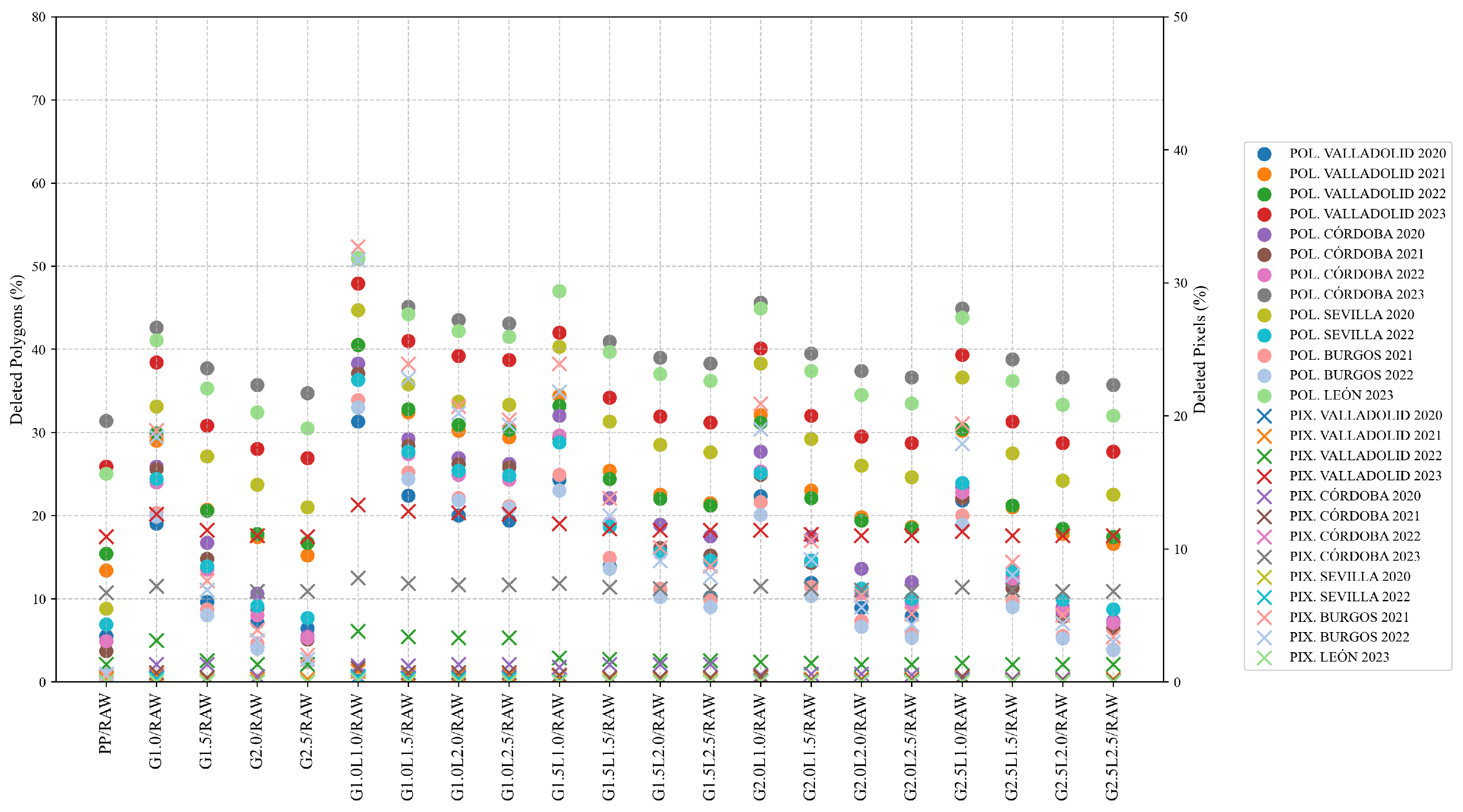
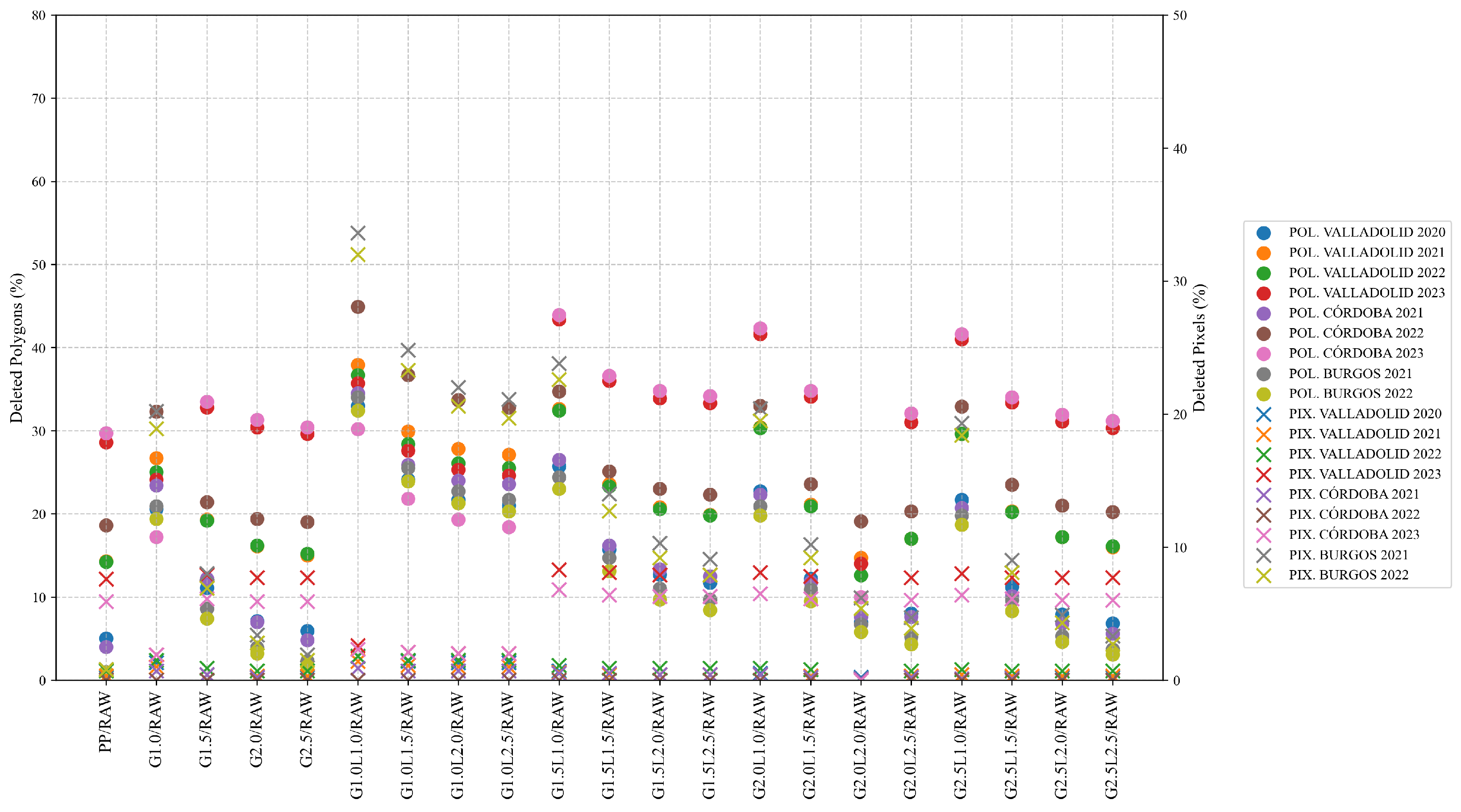
Different levels of data cleaning were applied to all available datasets. Figure 6 and Figure 7 show the percentage of data removed after the cleaning process. In the case of wheat (Figure 6), erasing outliers related to potential yield and combine harvester measurement limitations (PP) translated into elimination of 0.5% and 31.4% at the polygon level and 0% and 10.9% at the pixel level. Among the remaining data-cleaning levels, G1.0L1.0 was the most restrictive, removing between 31.3% and 51.0% of the data at the polygon level and up to 32.7% at the pixel level. The same trend can be observed for barley datasets (Figure 7), erasing 0.9% and 29.7% at the polygon level and 0% and 7.6% at the pixel level in the PP level and erasing the more restrictive level of cleaning (G1.0L1.0) between 30.8% and 44.9% of the data at polygon level and a maximum 33.6% at pixel level.

Although some cleaning filters remove a large proportion of polygon-level observations, the loss is less after resampling to a standard 10 × 10 m grid (pixel level), because the yield layers in polygons correspond to irregular segments, and consideration at the pixel level homogenizes the spatial resolution, reducing the influence of the reduced segments.

The CVs of the raw yield datasets ranged from 34.9% to 424.1% in wheat datasets and 34.4% to 362.9% in barley datasets. After applying the different cleaning levels, the CV ranged from 4.9% to 80.1% and 12.6% to 74.9% for wheat and barley datasets, respectively. The effect of data cleaning is equal across both crops in all datasets studied, increasing the mean and median values while reducing the CV and standard deviation.

Table 6. Summary of statistics for each type of yield data of wheat in Córdoba (2021).

Type	Mean	Median	SD	CV	Skew	Kurt
Raw	3453.3	3579.4	1300.7	41.6	0.6	10.9
PP	3559.7	3622.5	1246.4	35.0	−0.1	0.6
G1.0	3943.3	3889.0	700.5	17.8	0.5	0.3
G1.5	3949.3	3894.0	771.9	19.5	0.5	0.5
G2.0	3932.8	3883.0	811.7	20.6	0.4	0.8
G2.5	3915.3	3874.0	834.3	21.3	0.3	0.9
G1.0L1.0	3944.3	3890.5	688.0	17.4	0.5	0.2
G1.0L1.5	3946.8	3891.0	699.3	17.7	0.5	0.3
G1.0L2.0	3945.1	3891.0	701.0	17.8	0.5	0.3
G1.0L2.5	3944.1	3889.5	700.8	17.8	0.5	0.3
G1.5L1.0	3949.8	3891.0	742.8	18.8	0.5	0.5
G1.5L1.5	3953.1	3895.0	764.2	19.3	0.5	0.5
G1.5L2.0	3952.1	3896.0	769.5	19.5	0.5	0.5
G1.5L2.5	3950.5	3894.0	770.8	19.5	0.5	0.5
G2.0L1.0	3939.3	3885.0	773.8	19.6	0.5	0.8
G2.0L1.5	3943.6	3889.0	796.8	20.2	0.4	0.8
G2.0L2.0	3941.2	3888.0	805.0	20.4	0.4	0.8
G2.0L2.5	3938.2	3887.5	808.6	20.5	0.4	0.8
G2.5L1.0	3928.3	3877.0	789.1	20.1	0.4	0.9
G2.5L1.5	3932.7	3883.0	813.8	20.7	0.4	0.9
G2.5L2.0	3928.3	3881.0	825.8	21.0	0.3	0.9
G2.5L2.5	3924.4	3881.0	830.3	21.2	0.3	0.9

and

Table 7. Summary of statistics for each type of yield data of barley in Valladolid (2020).

Type	Mean	Median	SD	CV	Skew	Kurt
Raw	3657.4	3587.3	2050.0	56.1	1.0	10.8
PP	3797.6	3718.0	1858.3	48.9	0.3	−0.5
G1.0	4030.5	4150.0	1593.9	39.5	0.1	−0.8
G1.5	4021.0	4138.0	1627.2	40.5	0.1	−0.7
G2.0	4009.6	4107.0	1633.6	40.7	0.1	−0.7
G2.5	4003.3	4093.0	1633.3	40.8	0.1	−0.7
G1.0L1.0	4033.6	4142.0	1601.2	39.7	0.1	−0.8
G1.0L1.5	4033.6	4149.0	1600.6	39.7	0.1	−0.8
G1.0L2.0	4033.0	4151.0	1597.6	39.6	0.1	−0.8
G1.0L2.5	4031.9	4150.0	1596.0	39.6	0.1	−0.8
G1.5L1.0	4023.3	4145.0	1629.6	40.5	0.1	−0.8
G1.5L1.5	4025.3	4140.0	1630.7	40.5	0.1	−0.7
G1.5L2.0	4024.5	4143.0	1630.1	40.5	0.1	−0.7
G1.5L2.5	4023.4	4140.0	1628.7	40.5	0.1	−0.7
G2.0L1.0	4011.6	4115.0	1635.9	40.8	0.0	−0.8
G2.0L1.5	4015.1	4115.0	1637.7	40.8	0.1	−0.8
G2.0L2.0	4014.1	4115.0	1637.2	40.8	0.1	−0.7
G2.0L2.5	4012.7	4113.0	1635.7	40.8	0.1	−0.7
G2.5L1.0	4007.0	4106.0	1634.1	40.8	0.1	−0.8
G2.5L1.5	4009.8	4106.0	1636.4	40.8	0.1	−0.7
G2.5L2.0	4008.0	4100.0	1636.4	40.8	0.1	−0.7
G2.5L2.5	4006.2	4097.0	1635.1	40.8	0.1	−0.7

show an example of a summary of statistics for wheat and barley, respectively. When compared to the raw dataset, the cleaning process translates into an increase in the mean (ranging from 13.4% to 15.5%, and 9.5% to 10.3% for the wheat and barley presented examples) and median (ranging from 8.2% to 8.8%, and 14.1% to 15.7% for the wheat and barley presented examples), and a decrease in the standard deviation (ranging from 35.9% to 47.1%, and 20.1% to 22.2% for the wheat and barley presented examples) and CV (ranging from 48.8% to 58.1%, and 27.2% to 29.4% for the wheat and barley presented examples).

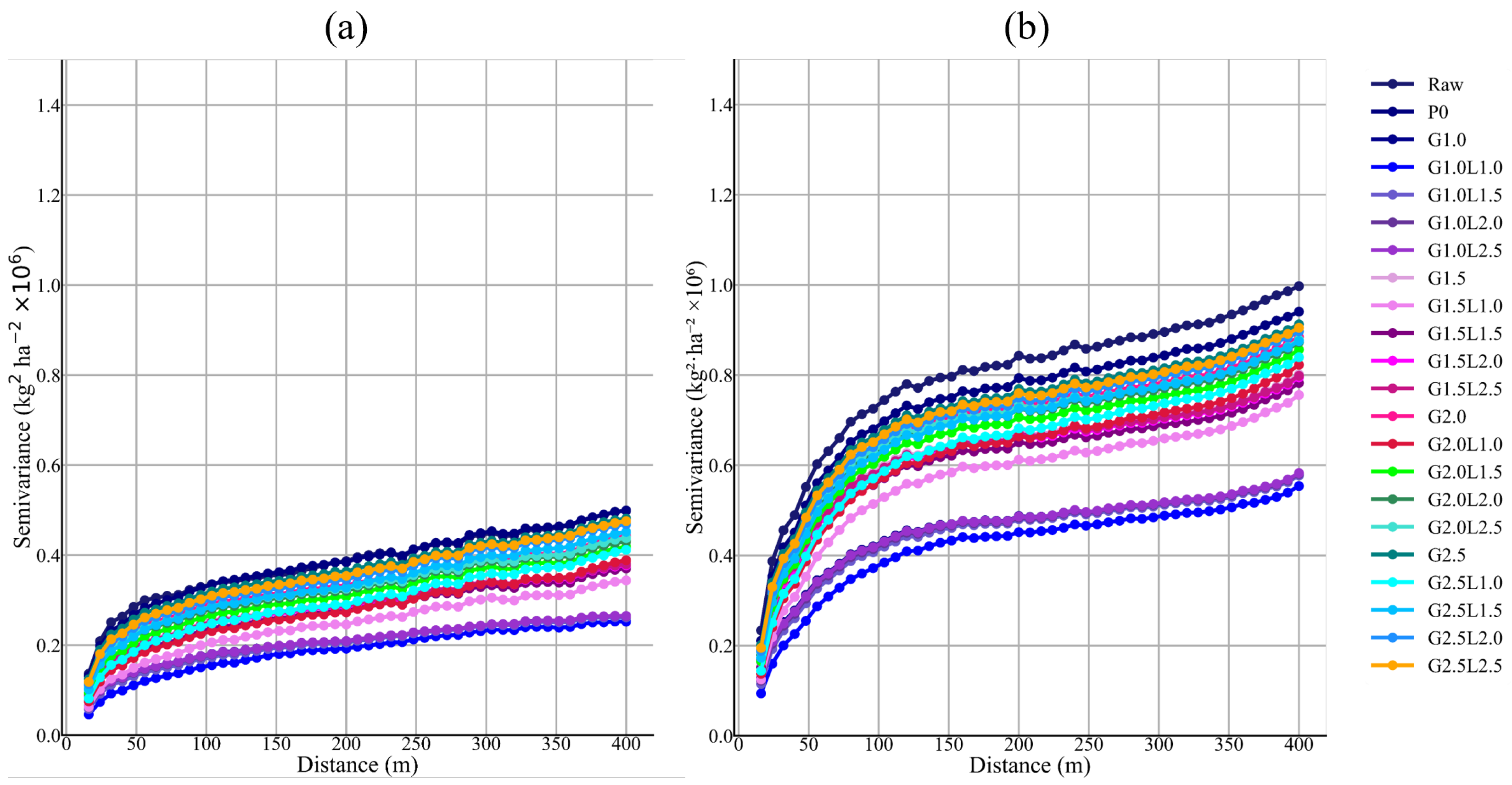
Concerning the spatial structure of the datasets, the structure of the data improved in all the datasets as the cleaning process was more restrictive, being the levels of cleaning process that incorporated a global filtering, with an n value of 1.0 (G1.0 family of cleaning), the ones that improved the spatial structure of the yield datasets the most. Figure 8 shows two examples of semivariograms, one for the wheat dataset (Figure 8a) and another for the barley dataset (Figure 8b). In both examples, it is evident that there were two separate groups in terms of spatial structure. However, the cleaning level G1.5L1.0 is between the two groups, so it should be carefully considered.

The results of this study highlight how restrictive cleaning levels reduce both nugget and sill, demonstrating the importance of cleaning protocols for improving measurement consistency and motivating researchers to consider these factors in their work. Additionally, it is noteworthy that the estimated range remains comparable between the different cleaning protocols, maintaining the spatial dimension of yields.

The improvement in spatial structure was reflected in a progressive increase in the fields normally distributed in the datasets. In this sense, P0 48% of the wheat fields and 50% of the barley fields presented a normal distribution. After applying the less restrictive level of cleaning (G2.5), these percentages increased to 64.8% and 56.1% for wheat and barley, respectively. The most restrictive cleaning level (G1.0L1.0), presented a percentage of normal field distribution of 79.4% in wheat and 73.5% in barley. The levels G1.0L2.5 and G1.5L1.0 presented, respectively, percentages of 82.9% and 71.9% in wheat, and 78.7% and 66.1% in barley. Among all the proposed cleaning levels, G1.0L2.5 was the one that increased the percentage of fields with a normal distribution the most.

In view of all these results, some of the levels of cleaning can be discarded, having to decide on the most suitable cleaning process, comparing the final map quality of five levels of cleaning: the G1.0 level with local filtering and G1.5L1.0.

3.3. Validation of Final Yield Quality

Two ML models were evaluated: partial least squares regression (PLSR), a multivariate statistical technique that combines principal component analysis and multiple linear regression, using Sentinel-2 bands and the yield of the two crops; and XGBoost, an open-source ML model that implements gradient-boosted decision tree algorithms. In this study, PLSR was fitted using 30 components (without scaling), while XGBoost used 50 trees with a maximum depth of 3 and a learning rate of 0.05 (random seed = 0).

Table 8. Performance of the trained models using PLSR and XGBoost algorithms for Raw, PP, and the preselected cleaning levels for wheat in Córdoba (2021).

Data Type		PLSR			XGBoost
		R2	MAE	RMSE	R2	MAE	RMSE
			kg ha−1			kg ha−1
Raw	Training	0.74	292.79	420.31	0.76	285.90	399.38
	Testing	0.68	343.40	473.48	0.65	364.90	497.48
PP	Training	0.73	299.86	426.56	0.76	292.20	401.94
	Testing	0.67	359.49	477.59	0.66	364.66	485.83
G1.0L1.0	Training	0.84	204.99	273.65	0.84	203.48	266.03
	Testing	0.81	226.01	300.80	0.81	240.47	305.48
G1.0L1.5	Training	0.82	218.83	291.61	0.83	215.64	281.63
	Testing	0.79	240.87	319.30	0.81	234.25	305.93
G1.0L2.0	Training	0.81	223.70	297.42	0.83	219.37	286.13
	Testing	0.79	246.38	325.81	0.80	240.33	312.99
G1.0L2.5	Training	0.81	224.98	298.74	0.83	219.92	286.62
	Testing	0.78	247.55	327.63	0.80	242.28	314.58
G1.5L1.0	Training	0.81	229.46	317.81	0.82	230.10	309.10
	Testing	0.80	239.65	335.17	0.77	260.39	355.59

and

Table 9. Performance of the trained models using PLSR and XGBoost algorithms for Raw, PP, and the preselected cleaning levels for barley in Valladolid (2020).

Data Type		PLSR			XGBoost
		R2	MAE	RMSE	R2	MAE	RMSE
			kg ha−1			kg ha−1
Raw	Training	0.82	511.68	687.35	0.84	484.09	651.87
	Testing	0.83	512.16	681.57	0.84	488.50	652.91
PP	Training	0.84	493.28	655.74	0.85	465.44	618.57
	Testing	0.83	506.20	652.82	0.85	470.50	619.50
G1.0L1.0	Training	0.89	415.78	530.90	0.90	389.38	497.80
	Testing	0.88	424.23	545.37	0.90	396.23	507.98
G1.0L1.5	Training	0.88	428.74	545.60	0.90	402.11	512.71
	Testing	0.88	425.79	542.82	0.89	405.71	517.73
G1.0L2.0	Training	0.88	430.49	547.14	0.90	404.17	514.29
	Testing	0.88	429.90	553.44	0.89	417.02	532.90
G1.0L2.5	Training	0.88	431.49	549.02	0.89	405.34	516.34
	Testing	0.88	430.26	553.91	0.89	417.72	534.57
G1.5L1.0	Training	0.87	441.99	573.70	0.89	416.84	541.11
	Testing	0.87	443.58	586.74	0.88	424.47	557.62

show examples of the performance of trained models using the final yield as the target variable and the data of the reflectance bands of Sentinel-2 for all available dates. The tendency observed in the results of the presented examples can be extrapolated to the remaining datasets. Only the results of the models trained for the pre-selected cleaning levels, as well as the PP and Raw data, are shown. In both crops, the XGBoost algorithm achieved the best performance during training, followed by the PLSR models, whose results were remarkably similar to those of XGBoost. The performance of the PLSR and XGBoost models on the test dataset is similar to that on the training dataset. Comparing the results for both crops, the R² values in the barley models are higher, while the RMSE and MAE values are higher than in the wheat cases.

Regarding the quality of the final yield datasets, the different cleaning levels presented a similar performance. So, the less restrictive levels (G1.0L2.5 and G1.5L1.0) presented in Table 8 and Table 9 must be more convenient for data erasure.

3.4. Comparison of Selected Cleaning Level with Common Yield Cleaning Method

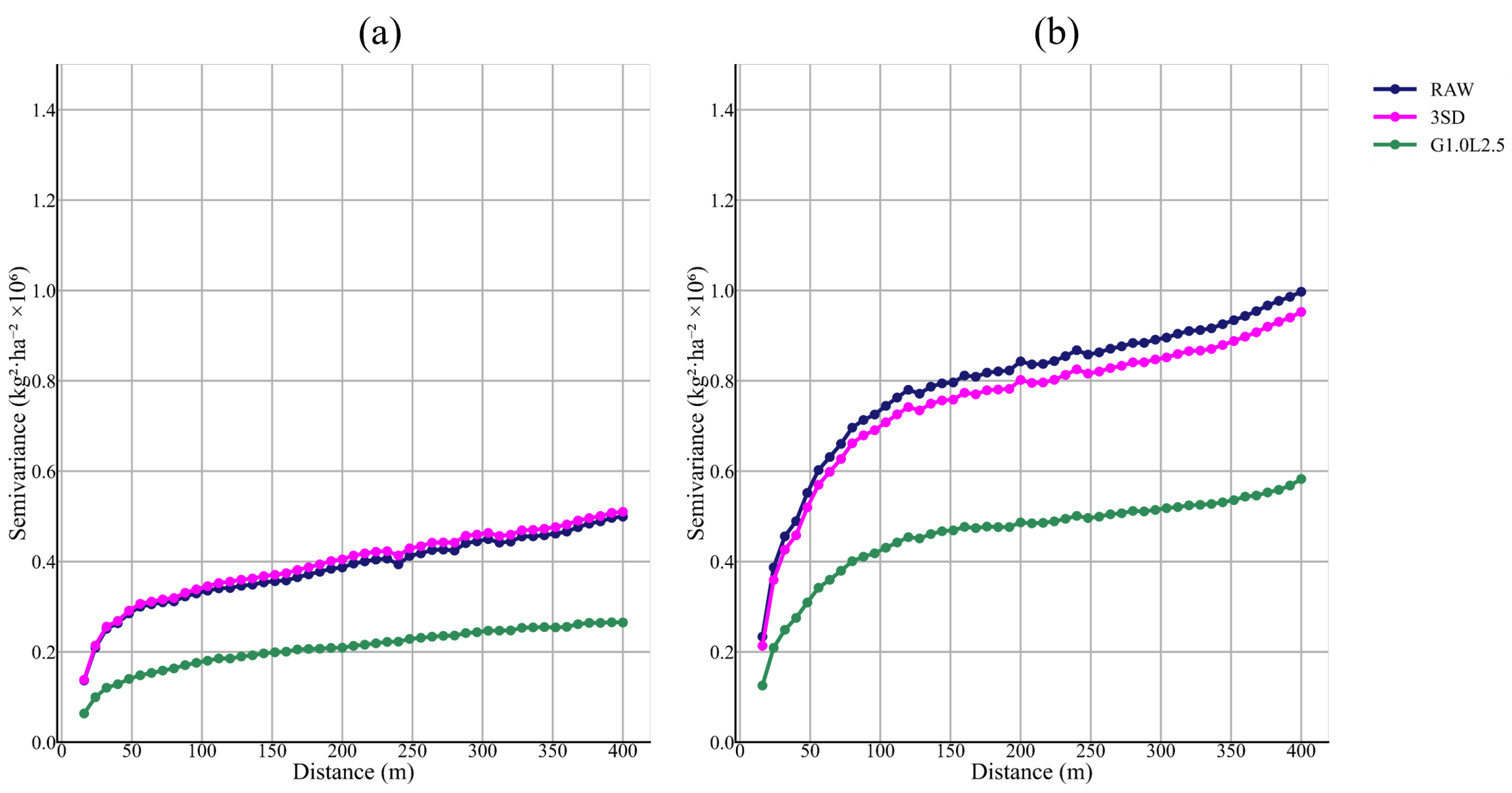
The selected data cleaned level (G1.0L2.5) and the RAW data were compared with a yield cleaning method commonly used in the literature (3SD). In terms of summary of statistics, it can be seen how for wheat (

Table A3. Comparison of statistics RAW, 3SD, and G1.0L2.5 yield data of wheat in Córdoba (2021).

Type	Mean	Median	SD	CV	Skew	Kurt
Raw	3453.3	3579.4	1300.7	41.6	0.6	10.9
3SD	3895.6	3866.5	859.9	22.1	0.2	1.1
G1.0L2.5	3944.1	3889.5	700.8	17.8	0.5	0.3

of Appendix B) and barley (

Table A4. Comparison of statistics RAW, 3SD, and G1.0L2.5 yield data of barley in Valladolid (2020).

Type	Mean	Median	SD	CV	Skew	Kurt
Raw	3657.4	3587.3	2050.0	56.1	1.0	10.8
3SD	3988.9	4075.0	1644.1	41.2	0.1	−0.7
G1.0L2.5	4031.9	4150.0	1596.0	39.6	0.1	−0.8

of Appendix B), the conservative method (3SD) has a higher mean and median, and a lower SD and CV when compared with the raw data, but the statistics are slightly better for the selected cleaning level, especially in terms of SD. In the 3SD method, the % of deleted data improves compared to G1.0L2.5, deleting 3SD by 2.7 and 3.1%, and G1.0G2.5 by 25.8 and 22.4% for wheat and barley, respectively. However, in the case of spatial structure (Figure A1 of Appendix B), it can be seen that 3SD does not improve spatial structure much compared to the RAW data. Regarding ML model execution, 3SD performed better than RAW, but G1.0L2.5 had the highest R² values and the lowest RMSE and MAE for both training and testing. Finally, after the 3SD method, 44.0% and 55.6% of the fields showed a normal distribution, a significantly lower percentage than that achieved by the proposed and selected cleaning method in this study.

4. Discussion

The results of the descriptive analysis of the datasets justify the non-normal distribution of the Raw datasets. It also confirms that removing combine harvester overlaps, GPS errors, and yield values outside the possible biological range improves the distribution, increasing the number of fields with a normal distribution in the datasets (from 8.2% to 36.9% of fields, depending on location and crop type). In view of these results, other authors, such as Aworke et al. [27], have applied data transformations (e.g., logarithmic transformation) to obtain a dataset with a normal distribution. However, those transformations are usually used with small datasets containing few fields. When these transformations are applied to large datasets, as shown in Table 4, it is evident that this method cannot be applied to all datasets. Therefore, the use of the preprocessed datasets (P0) for the proposed data cleaning processes is highly recommended. The non-normal distribution of the datasets is accounted for, as the proposed approach uses statistics that are not overly influenced by extreme values (Sainani, 2012) [17].

Other authors like Blasch et al. [9], Sun et al. [4], Ping et al. [12], Robinson and Metternicht [25], and Gozdowski et al. [11] have emphasized that the combine harvester has a minimum value of yield that it can measure accurately. For winter cereals such as wheat and barley, the minimum value has been set in the range of 100 and 1000 kg ha⁻¹, but the criteria to set one value or another have not yet been explained. The study of the CV_median for each range of yield (Table 5) helped to set this minimum in 500 kg ha⁻¹. This decision can be explained from a mathematical point of view: for an increasing range of values, the mean tends to increase while the standard deviation remains similar, resulting in a higher CV_median and yield ranges with lower yields. However, the CV_median of the range of yield from 0 to 500 kg ha⁻¹ is too high when compared to the next studied range (500 to 1000 kg ha⁻¹), indicating an unusually high standard deviation.

In terms of total erased data at polygon level, the results obtained are aligned with those obtained by other authors, deleting a percentage of data between 10% and 50% [4,6,7,11,12,24,26]. However, if the cleaned yield data is resampled and used with Sentinel-2 at higher spatial resolution, the percentage of deleted data decreases, reaching a maximum of 33.6% of the 10 × 10 m pixels (pixel level). Given concerns about potential bias, the proposed filtering protocol is applied to each field using the median and interquartile range at the global and 40 m neighborhood levels, with the aim of reducing inconsistent values. To validate this measure, not only were statistical indicators used, but semivariograms and validation tests were also reported.

The removal of global outliers and local inliers significantly modified the summary of statistics of the datasets by lowering the CV (34.4–424.1% in the Raw dataset to 4.9–80.1% after cleaning) and standard deviation (22–64%) and increasing the value of mean (9.5–15.5%) and median (8.2–15.7%). Vega et al. [6] reported a similar decrease in CV, with the datasets’ CV ranging from 88% to 213% before cleaning and from 34% to 46% after cleaning. Other authors have also reported increases of 6–15% in the mean and decreases of 22–64% in the standard deviation, similar to Lyle et al. [28], who reported increases of 11% and decreases of 47% in the mean and standard deviation, respectively. The increase in the median was also revealed in different crops, reducing the differences between mean and median yield [12,24], observing in winter wheat differences < 160 kg ha⁻¹ [7]. Considering that a good cleaning method should increase the normality of the distribution of the yield data [14,24,25], these reduced differences between mean and median yield were reflected in the rise of studied yields that present a normal distribution of data, with a maximum value of 82.9% and 78.7% (G1.0L2.5 cleaning level) of the total wheat and barley fields, respectively. Although the proposed protocols cause an increase in elements that meet normality criteria (skewness, −0.5 and 0.5; kurtosis, −2 and 2), another significant group remained outside these thresholds in the most effective method (G1.0L2.5). Residual non-normality does not indicate a sensor or processing system effect, since the yield image values may reflect the influence of the field’s physical environment and crop management on crop productivity. Consequently, anomalous and obvious data could be eliminated using statistical indicators that do not assume strict normality. Moreover, the uncertainty has been reduced after applying the cleaning protocol to the yield datasets, as shown by a substantial reduction in the nugget value [25] in each proposed cleaned level, being the levels of cleaning of the G1.0 family with local filtering, and G1.5L1.0 the ones that better improved the spatial structure of the yield datasets. In addition, lag distance at which the sill is achieved in the semivariograms is consistent across all proposed cleaning levels, presenting a downward shift in the total semivariance, as observed by Sun et al. [4]. Therefore, the downward shift in the semivariance is consistent with the elimination of error. At the same time, the semivariogram’s stable range indicates that the spatial dimension of the yield distribution is maintained.

Yield data is a precious source of information for precision agriculture, and therefore, proper cleaning is fundamental to its reliable use. In this context, its use to develop yield prediction models is a common practice. The use of ML to develop prediction models has shown good results, and these techniques are less affected by errors than regression models [29]. The execution of the two applied ML algorithms helped achieve a balance between cleaning level and prediction quality, as other authors have reported [15]. All the preselected cleaning levels performed similarly during training for both algorithms, yielding better results than the models trained with Raw and PP yield data. In addition, when the models’ performance is evaluated on the test data, it is evident that R² values decrease, while RMSE and MAPE increase substantially in the Raw and PP models, indicating clear overfitting and highlighting the poor quality of the data. The performance of the models trained with the pre-selected cleaning levels remains similar when applied to the test data. The good execution of the models in training and testing, along with the similar results obtained between preselected cleaning levels, indicates that the less restrictive preselected cleaning levels (G1.0L2.5 and G1.5L1.0) are the most suitable protocols for cleaning yield data, as they also erase a lower percentage of yield data (maximum percentage of erased polygons of 42% in wheat and 33% in barley for G1.0L2.5, and maximum of 48% in wheat and 35% in barley for G1.5L1.0). In addition, the range of values continues being similar, while R² increases, also reflecting the improvement of the spatial structure of the data, while the RMSE and MAPE values decrease when compared with the crude data, but not substantially, highlighting that the behavioral patter of the data has not changed maintaining the real variability of yield data, and, subsequently, the cleaning process has not introduced bias in the data.

Between G1.0L2.5 and G1.5L1.0 levels of cleaning, the G1.0L2.5 is chosen as the better protocol for cleaning yield data, as the semivariograms have shown that the spatial structure of the cleaned data is better, and the percentage of fields presented a normal distribution is maximum when it is applied (82.9% in wheat and 78.7% in barley for G1.0L2.5, and maximum of 71.9% in wheat and 66.1% in barley for G1.5L1.0.

After choosing the better cleaning protocol, the results were compared with the ones obtained when a more conservative method, commonly found in the literature, is applied, the 3SD method. When both methods were compared, the G1.0L2.5 method significantly improved the spatial structure of the data and significantly increased the percentage of fields with a normal distribution of yield data.

The presented framework for yield data cleaning is proposed as an easily applied approach for cleaning yield data error measurements. As the protocol includes both global and local filtering, both outliers and inliers will be erased. The framework employs a parametric approach at both the global and local levels. However, since the unfiltered datasets do not follow a normal distribution, the median and interquartile range are used as filtering statistics, as the data distribution has less influence on them. The proposed cleaning method was tested on a large dataset across different locations, growing seasons, and two crops, yielding good results. It has lower computational requirements than more complex methods, and the cleaned data was used to train ML models with good results as a form of validation. Future studies should focus on applying the selected data-cleaning method to other locations and crops to assess the quality of the cleaned data and determine whether the same cleaning level can be applied to conditions not included in the present work.

5. Conclusions

The presented study proposes a data-cleaning methodology for yield data in wheat and barley crops, applied to a large dataset. Only georeferenced yield data was used in the proposed methodology, allowing the application to all yield maps generated by the YieldTrack software. Firstly, biological outliers and measurements below 500 kg ha⁻¹ are deleted. Secondly, low-computational-expense parametric global and local filtering is applied, using statistics robust to non-normally distributed data (median and interquartile range). Four different limit coefficients were used for global and local filtering, yielding in 20 cleaning levels, which were compared to select the optimal one. The percentage of deleted data, the spatial structure, a descriptive analysis of the data, and the performance of machine learning models trained and tested on clean data and Sentinel-2 reflectance data were used to select the best approach.

The selected level was the G1.0L2.5. This cleaning method was among the most effective in improving the spatial structure of the data and the predictive performance of machine learning models. The maximum percentage of polygons deleted was 42% and 33% for wheat and barley, respectively, and the percentage of fields that showed a normal distribution after filtering was highest at 82.9% and 78.7% for wheat and barley, respectively. The use of the selected method increased the mean and median of the datasets, and decreased the standard deviation and CV values.

Future work will focus on applying the selected cleaning method to other locations and crops, as well as to the Yield Track software, and on evaluating the quality of the cleaned data not included in the present study. In addition, the results of the present work will enable the development of early yield-prediction models that producers can use to implement site-specific crop management and apply correction measures when necessary.

This approach will enable the training of predictive models for advanced phenological stages, which can be applied to estimate cereal production. These estimations contribute to Sustainable Development Goal 2 (Zero Hunger) by improving food security and agricultural planning, and to Sustainable Development Goal 8 (Decent Work and Economic Growth) by reducing market uncertainty and facilitating risk management.

References

1. Nations, U. Population, 2025. Available online: https://www.un.org/en/global-issues/population (accessed on 19 October 2025).
2. Bruinsma, J. World Agriculture: Towards 2015/2030; Routledge: London, UK, 2017. [Google Scholar] [CrossRef]
3. Billen, G.; Lassaletta, L.; Garnier, J. A biogeochemical view of the global agro-food system: Nitrogen flows associated with protein production, consumption and trade. Glob. Food Secur. 2014, 3, 209–219. [Google Scholar] [CrossRef]
4. Sun, W.; Whelan, B.; McBratney, A.B.; Minasny, B. An integrated framework for software to provide yield data cleaning and estimation of an opportunity index for site-specific crop management. Precis. Agric. 2013, 14, 376–391. [Google Scholar] [CrossRef]
5. Arizo-García, P.; Castiñeira-Ibáñez, S.; Tarrazó-Serrano, D.; Franch, B.; Rubio, C.; San Bautista, A. Use of Sentinel-2 Images to Elaborate a VRT Sensor-Based and Map-Based Nitrogen Fertilization in Wheat and Barley Crops. Appl. Sci. 2025, 15, 11646. [Google Scholar] [CrossRef]
6. Vega, A.; Córdoba, M.; Castro-Franco, M.; Balzarini, M. Protocol for automating error removal from yield maps. Precis. Agric. 2019, 20, 1030–1044. [Google Scholar] [CrossRef]
7. Leroux, C.; Jones, H.; Clenet, A.; Dreux, B.; Becu, M.; Tisseyre, B. A general method to filter out defective spatial observations from yield mapping datasets. Precis. Agric. 2018, 19, 789–808. [Google Scholar] [CrossRef]
8. Córdoba, M.A.; Bruno, C.I.; Costa, J.L.; Peralta, N.R.; Balzarini, M.G. Protocol for multivariate homogeneous zone delineation in precision agriculture. Biosyst. Eng. 2016, 143, 95–107. [Google Scholar] [CrossRef]
9. Blasch, G.; Li, Z.; Taylor, J.A. Multi-temporal yield pattern analysis method for deriving yield zones in crop production systems. Precis. Agric. 2020, 21, 1263–1290. [Google Scholar] [CrossRef]
10. Fita, D.; Rubio, C.; Franch, B.; Castiñeira-Ibáñez, S.; Tarrazó-Serrano, D.; San Bautista, A. Improving harvester yield maps postprocessing leveraging remote sensing data in rice crop. Precis. Agric. 2025, 26, 33. [Google Scholar] [CrossRef]
11. Gozdowski, D.; Samborski, S.; Dobers, E.S. Evaluation of Methods for the Detection of Spatial Outliers in the Yield Data of Winter Wheat. In Proceedings of the Colloquium Biometricum. Uniwersytet Przyrodniczy w Lublinie, Katedra Zastosowań Matematyki i Informatyki, 2010, Number 40. Available online: https://bibliotekanauki.pl/articles/9643 (accessed on 15 December 2023).
12. Ping, J.L.; Dobermann, A. Processing of Yield Map Data. Precis. Agric. 2005, 6, 193–212. [Google Scholar] [CrossRef]
13. Sudduth, K.A.; Drummond, S.T. Yield Editor: Software for Removing Errors from Crop Yield Maps. Agron. J. 2007, 99, 1471–1482. [Google Scholar] [CrossRef]
14. Natale, A.; Antognelli, S.; Ranieri, E.; Cruciani, A.; Boggia, A. A Novel Cleaning Method for Yield Data Collected by Sensors: A Case Study on Winter Cereals. In Computational Science and Its Applications – ICCSA 2020; Springer International Publishing: Cham, Switzerland, 2020; pp. 684–691. [Google Scholar] [CrossRef]
15. Sanchez, C.; Pathak, D.; Miranda, M.; Charfuelan, M.; Helber, P.; Nuske, M.; Bischke, B.; Habelitz, P.; Rahman, N.; Mena, F.; et al. Influence of Data Cleaning Techniques on Sub-Field Yield Predictions. In Proceedings of the IGARSS 2023-2023 IEEE International Geoscience and Remote Sensing Symposium, Pasadena, CA, USA, 16–21 July 2023; IEEE: Piscataway, NJ, USA, 2023; Volume 13, pp. 4852–4855. [Google Scholar] [CrossRef]
16. Jain, S.; Shukla, S.; Wadhvani, R. Dynamic selection of normalization techniques using data complexity measures. Expert Syst. Appl. 2018, 106, 252–262. [Google Scholar] [CrossRef]
17. Sainani, K.L. Dealing with Non-normal Data. PM&R 2012, 4, 1001–1005. [Google Scholar] [CrossRef]
18. López-Bellido, L. Cereales, Cultivos Herbáceos; Escuela Técnica Superior de Ingenieros Agrónomos, Universidad de Córdoba: Córdoba, Spain, 1991; Volume 1. [Google Scholar]
19. López-Bellido, R.J.; López-Bellido, L.; Benítez-Vega, J.; López-Bellido, F.J. Tillage system, preceding crop, and nitrogen fertilizer in wheat crop: II. Water utilization. Agron. J. 2007, 99, 66–72. [Google Scholar] [CrossRef]
20. IGME. Web Map Viewer, 2023. Available online: https://igme.maps.arcgis.com/home/webmap/viewer.html?useExisting=1 (accessed on 26 September 2025).
21. European Space Agency. Sentinel-2 User Handbook. Technical Report, ESA, 2015. ESA Standard Document. Available online: https://sentinels.copernicus.eu/documents/247904/685211/Sentinel-2_User_Handbook (accessed on 15 December 2025).
22. Kappal, S. Data Normalization Using Median & Median Absolute Deviation (MMAD) based Z-Score for Robust Predictions vs. Min–Max Normalization. Lond. J. Res. Sci. Nat. Form. 2019, 19, 39–44. [Google Scholar] [CrossRef]
23. Atkinson, A.C.; Riani, M.; Corbellini, A. The Box–Cox Transformation: Review and Extensions. Stat. Sci. 2021, 36, 239–255. [Google Scholar] [CrossRef]
24. Maldaner, L.F.; Molin, J.P. Data processing within rows for sugarcane yield mapping. Sci. Agric. 2020, 77, e20180391. [Google Scholar] [CrossRef]
25. Robinson, T.; Metternicht, G. Comparing the performance of techniques to improve the quality of yield maps. Agric. Syst. 2005, 85, 19–41. [Google Scholar] [CrossRef]
26. Řezník, T.; Herman, L.; Trojanová, K.; Pavelka, T.; Leitgeb, Š. Interpolation of Data Measured by Field Harvesters: Deployment, Comparison and Verification. In Environmental Software Systems. Data Science in Action; Springer International Publishing: Cham, Switzerland, 2020; pp. 258–270. [Google Scholar] [CrossRef]
27. Aworka, R.; Cedric, L.S.; Adoni, W.Y.H.; Zoueu, J.T.; Mutombo, F.K.; Kimpolo, C.L.M.; Nahhal, T.; Krichen, M. Agricultural decision system based on advanced machine learning models for yield prediction: Case of East African countries. Smart Agric. Technol. 2022, 2, 100048. [Google Scholar] [CrossRef]
28. Lyle, G.; Bryan, B.A.; Ostendorf, B. Post-processing methods to eliminate erroneous grain yield measurements: Review and directions for future development. Precis. Agric. 2013, 15, 377–402. [Google Scholar] [CrossRef]
29. Neutatz, F.; Chen, B.; Alkhatib, Y.; Ye, J.; Abedjan, Z. Data Cleaning and AutoML: Would an Optimizer Choose to Clean? Datenbank-Spektrum 2022, 22, 121–130. [Google Scholar] [CrossRef]
Figure 1. Location of the studied data. The fields studied are outlined in red for wheat and pink for barley, for each location and growing season presented.
Agronomy 16 00386 g001
Figure 2. Representation of the yield data in (a) TOPCON software and (b) Trimble software.
Agronomy 16 00386 g002
Figure 3. Two-stage workflow used in this study. Stage 1: Raw to P0 (biological limits), distribution/transformations to PP. Stage 2: PP to global (G) and local (L) filtering, combinations (GL), and comparison of cleaning levels to select the optimal protocol.
Agronomy 16 00386 g003
Figure 4. Proposed parametric cleaning procedure applied to PP data. Global adjustment uses field median ( α ) and IQR ( β ) to define bounds (Equations (2) and (3)) for n = 1.0–2.5 (G1.0–G2.5). Local adjustment uses neighborhood median ( γ ) and IQR ( δ ) within a 40 m radius (Equations (4) and (5)) to test L1.0–L2.5, producing 16 G × L combinations. All outputs are rescaled to a 10 × 10 m grid by averaging values within each pixel. The dotted box indicates that all the levels of cleaned data within it were rescaled, not only those obtained after applying the local adjustment.
Agronomy 16 00386 g004
Figure 5. Box-whisker plots of datasets yield the standard deviation as a function of the local adjustment search radius at a field example. Red lines indicate the median standard deviation for each box-whisker; white boxes indicate the mean standard deviation for each group; and black circles represent anomalous data.
Agronomy 16 00386 g005
Figure 6. Percentage of erased data in the different cleaning levels at polygon and pixel level for wheat datasets.
Agronomy 16 00386 g006
Figure 7. Percentage of erased data in the different cleaning levels at polygon and pixel level for barley datasets.
Agronomy 16 00386 g007
Figure 8. Semivariograms for all proposed cleaning levels using an example dataset: (a) wheat (Córdoba, 2021) and (b) barley (Valladolid, 2020).
Agronomy 16 00386 g008