Article

Monitoring Wolfberry (Lycium barbarum L.) Canopy Nitrogen Content with Hyperspectral Reflectance: Integrating Spectral Transformations and Multivariate Regression

1
School of Civil and Hydraulic Engineering, Ningxia University, Yinchuan 750021, China
2
Institute of Agricultural Economy and Information Technology, Ningxia Academy of Agriculture and Forestry Sciences, Yinchuan 750002, China
3
Ningxia Research Center for Smart Agriculture Engineering and Technology, Yinchuan 750002, China
4
Department of Water Resources, China Institute of Water Resources and Hydropower Research, Beijing 100038, China
5
Ningxia Academy of Building Research Co., Ltd., Yinchuan 750021, China
*
Authors to whom correspondence should be addressed.
Agronomy 2025, 15(9), 2072; https://doi.org/10.3390/agronomy15092072
Submission received: 2 July 2025 / Revised: 18 August 2025 / Accepted: 26 August 2025 / Published: 28 August 2025
(This article belongs to the Section Precision and Digital Agriculture)

Abstract

Accurate monitoring of canopy nitrogen content in wolfberry (Lycium barbarum L.) is essential for optimizing fertilization management, improving crop yield, and promoting sustainable agriculture. However, the sparse, architecturally complex canopy of this perennial shrub—featuring coexisting branches, leaves, flowers, and fruits across maturity stages—poses significant challenges for canopy spectral-based nitrogen assessment. This study integrates methods across canopy spectral acquisition, transformation, feature spectral selection, and model construction, and specifically explores the potential of hyperspectral remote sensing, integrated with spectral mathematical transformations and machine learning algorithms, for predicting canopy nitrogen content in wolfberry. The overarching goal is to establish a feasible technical framework and predictive model for monitoring canopy nitrogen in wolfberry. In this study, canopy spectral measurements are systematically collected from densely overlapping leaf regions within the east, south, west, and north orientations of the wolfberry canopy. Spectral data undergo mathematical transformation using first-derivative (FD) and continuum-removal (CR) techniques. Optimal spectral variables are identified through correlation analysis combined with Recursive Feature Elimination (RFE). Subsequently, predictive models are constructed using five machine learning algorithms and three linear regression methods. Key results demonstrate that (1) FD and CR transformations enhance the correlation with nitrogen content (max correlation coefficient (r) = −0.577 and 0.522, respectively; p < 0.01), surpassing original spectra (OS, −0.411), while concurrently improving model predictive capability. Validation tests yield maximum R2 values of 0.712 (FD) and 0.521 (CR) versus 0.407 for OS, confirming FD’s superior performance enhancement. (2) Nonlinear machine learning models, by capturing complex canopy-light interactions, outperform linear methods and exhibit superior predictive performance, achieving R2 values ranging from 0.768 to 0.976 in the training set—significantly outperforming linear regression models (R2 = 0.107–0.669). (3) The Random Forest (RF) model trained on FD-processed spectra achieves the highest accuracy, with R2 values of 0.914 (training set) and 0.712 (validation set), along with an RPD of 1.772. This study demonstrates the efficacy of spectral transformations and nonlinear regression methods in enhancing nitrogen content estimation. It establishes the first effective field monitoring strategy and optimal predictive model for canopy nitrogen content in wolfberry.

1. Introduction

Wolfberry, scientifically named Lycium barbarum L., is a perennial deciduous shrub characterized by its continuous flowering throughout its growth cycle. While it is distributed globally, it is predominantly cultivated in the arid and semi-arid regions of northwest China [1]. Owing to its remarkable ecological adaptability, wolfberry has emerged as a key cash crop in northwest China [2]. Its exceptional nutritional and medicinal properties further enhance its value. The Ningxia Hui Autonomous Region in northwest China is the species’ origin and main cultivation area. As Ningxia’s most distinctive agricultural industry, wolfberry plays a crucial role in addressing rural employment, increasing economic income, and maintaining environmental sustainability [3]. It also serves as Ningxia’s “red business card” both nationally and globally. Consequently, the sustainable development of the wolfberry industry has garnered significant attention from local authorities and communities.
Nitrogen is an essential component of chlorophyll, the green pigment that facilitates photosynthesis. Extensive research indicates a close correlation between nitrogen content in vegetation and photosynthetic efficiency and intensity, which are fundamental for biomass accumulation and crop yield and quality formation [4,5]. For wolfberry (Lycium barbarum L.), a high fertilizer-responsive cash crop with high demand for water and fertilizer inputs, nitrogen directly influences chlorophyll synthesis, leaf area development, and photosynthetic rate, thereby regulating fruit yield and quality [3,6]. Research demonstrates that optimal nitrogen application significantly enhances dry fruit production across diverse habitats. However, excessive application elevates production costs while inducing soil nutrient imbalance and environmental pollution, ultimately reducing both yield and fruit quality [3,6]. Thus, implementing effective nitrogen fertilization management strategies is imperative to promote reproductive growth, ensure high yields while maintaining superior quality, and enable cost-effective, eco-friendly cultivation. Accurate and rapid monitoring of nitrogen content in wolfberry tissues, particularly canopy nitrogen content, remains crucial for scientific fertilization.
The conventional approach to determining nitrogen content involves the Kjeldahl method, necessitating field sampling and laboratory processing (drying, weighing, grinding, sifting, and analysis) [7]. While accurate, this chemical analysis is inherently time-consuming, labour-intensive, costly, and inefficient; it cannot support rapid, non-destructive, real-time nitrogen monitoring [7]—underscoring the urgent need for advanced alternatives. To address these limitations, several techniques have been explored: SPAD sensors provide rapid leaf-level nitrogen estimates [8] but lack spatial coverage, as single-point measurements fail to represent whole-plant variability. Multispectral remote sensing offers broader coverage but limited spectral resolution, struggling to differentiate subtle nitrogen-related spectral variations [9]. Drone-based RGB imaging is cost-effective for large-scale monitoring but relies on indirect vegetation indices [10], which are easily confounded by environmental factors (e.g., lighting, canopy structure). Among these alternatives, hyperspectral remote sensing stands out for non-destructive monitoring of crop biophysical parameters. Its high spectral resolution (numerous contiguous narrow bands) enables differentiation of subtle spectral variations in vegetation [11], a capability unmatched by broader-spectrum techniques. For example, while SPAD sensors or multispectral systems might miss nuanced nitrogen signals, hyperspectral data can capture fine-scale spectral features associated with nitrogen content. Additionally, unlike leaf-scale assessments (e.g., SPAD measurements), canopy-scale hyperspectral measurements provide a more comprehensive representation of whole-plant nitrogen status [12]—critical for accurate field-scale nitrogen management. Thus, hyperspectral remote sensing balances precision, coverage, and practicality, addressing key limitations of both traditional laboratory methods and other proximal/remote sensing tools. This justifies its growing prominence in crop nitrogen monitoring.
Multiple strategies have been developed to suppress noise and enhance vegetation signatures in canopy spectra. Mathematical transformations (e.g., derivatives, continuum removal) applied to raw canopy reflectance data effectively reduce background interference, amplify spectral absorption features, and improve signal-to-noise ratio (SNR) and model accuracy [13,14,15,16]. Spectral indices, constructed by combining two or more characteristic bands through ratio-based or composite formulas, effectively enhance spectral absorption features associated with foliar biochemical concentrations [17,18]. Numerous studies have focused on screening sensitive spectral information and developing detection models to improve the prediction accuracy of crop nitrogen status [19].
Linear regression models continue to be the most prevalent approach for estimating crop physiological traits, owing to their simplicity and low computational requirements [18,20]. While these statistical regression methods effectively correlate nitrogen levels with canopy spectral data, advancements in computing power in recent years have facilitated the broader application of machine learning in precision agriculture [21]. Furthermore, given the great potential of machine learning algorithms to capture the complex relationships between spectra and nitrogen, their use in crop parameter estimation has become increasingly widespread [11,12,13,14,15,17,21]. An examination of relevant research findings reveals that prior research has predominantly concentrated on annual field crops, including rice [12,15], wheat [13,18,21,22], maize [23,24,25], cotton [4,17], potato [26], and soybean [11]. Although there are reports on apple [7,14] and litchi [27], research on perennial cash crops remains relatively scarce overall. In the case of wolfberries, Adria et al. employed hyperspectral imaging technology to detect and analyze the moisture content of dried wolfberries, demonstrating the feasibility of rapid, non-destructive detection of moisture levels in wolfberries using this technology [28]. Meanwhile, Zhao et al. utilized hyperspectral technology to estimate the canopy water content of wolfberries [29]. Their study employed simple linear regression alongside four multivariate statistical analysis algorithms—specifically ridge regression, least absolute shrinkage and selection operator, principal component regression, and partial least squares regression—to develop a monitoring model for wolfberry canopy water content, with a subsequent evaluation of modelling accuracy. We developed an optimized leaf-scale monitoring model for wolfberry nitrogen content using hyperspectral sensing [30]. To the best of our knowledge, there are currently no research reports on predicting wolfberry nitrogen content at the canopy scale using hyperspectral technology. To address this research gap in wolfberry nitrogen monitoring, the present study integrates both linear and nonlinear modelling approaches. Specifically, we employ three linear regression methods—Gradient Descent Linear Regression (GDLR), Ordinary Least Squares Linear Regression (OLSLR), and Ridge Regression (RR)—to capture potential linear relationships between spectral variables and nitrogen content. Additionally, five machine learning algorithms—Random Forest (RF), Adaptive Boosting (AdaBoost), Extremely Randomized Trees (Extra Trees), Categorical Boosting (CatBoost), and Extreme Gradient Boosting (XGBoost)—are utilized to explore nonlinear patterns, given their demonstrated effectiveness in handling complex spectral data and enhancing prediction accuracy for crop biophysical parameters [12,18]. By comparing the performance of these linear and nonlinear models, we aim to identify the optimal approach for estimating wolfberry canopy nitrogen content, thereby providing a robust methodological basis for practical applications.
Given the potential of hyperspectral sensing for agricultural nitrogen management and the critical need for science-based fertilizer regulation in economically significant wolfberry cultivation, this study proposes a practical strategy. This strategy aims to monitor wolfberry nitrogen content in the field using canopy hyperspectral reflectance and is implemented in five steps: (1) acquisition of canopy hyperspectral data and measurement of nitrogen content; (2) mathematical preprocessing of canopy hyperspectral data and comparative analysis of spectral characteristics; (3) identification of spectral features with high sensitivity to nitrogen content; (4) development of a multivariate regression model using the selected spectral features as predictors for estimating wolfberry leaf nitrogen content; (5) evaluation of model performance and predictive accuracy, followed by selection of the optimal model.

2. Materials and Methods

2.1. Study Area and Field Observation

The study areas are located in Zhongning County, within the Weining irrigation zone, and Nuanquan Farm in the northern part of Yinchuan City. These regions are recognized as primary wolfberry cultivation areas and are designated as the National Geographical Indication Product Protection Zone for Ningxia wolfberries. The region experiences a middle temperate arid climate, characterized by abundant light and thermal resources: annual sunshine duration of 2500–3000 h, solar radiation of 5925.3 MJ m−2 yr−1, effective accumulated temperatures (≥10 °C) of 2500–3000 °C, and significant diurnal temperature variations during the wolfberry growth period (daily range: 12.9–16.5 °C). These unique photothermal conditions significantly enhance photosynthesis, sugar accumulation, fruit coloration, and flavour development in wolfberries, contributing to their distinctive quality. As shown in Figure 1, the recorded meteorological data support these observations. The soil comprises irrigated silt or light calcareous soils, with a pH of 7.5–8.5, organic matter content >5 g kg−1, and total salt content <5 g kg−1. Its deep, fertile, and well-structured nature facilitates efficient irrigation and drainage, providing optimal conditions for wolfberry growth.
To comprehensively understand the growth dynamics of wolfberry trees throughout their phenological stages—a critical prerequisite for accurately monitoring the nitrogen nutrition levels of wolfberry plants—field observations were conducted in two distinct cultivation regions. Table 1 summarizes the phenological characteristics of selected wolfberry trees, which were chosen based on uniformity in variety and standardized cultivation practices. The study focused on “Ningqi No. 7”, a variety widely cultivated in Ningxia, with a planting configuration of 3 m row spacing and 1 m plant spacing. A drip irrigation system was installed, with pipes positioned 15 cm above ground level, supplying water sourced from the Yellow River and local wells. Field management practices, including pruning, weeding, fertilization, and irrigation, were carried out in accordance with local traditional agricultural practices.

2.2. Data Acquisition and Preprocessing

2.2.1. Canopy Hyperspectral Reflectance Acquisition

Canopy spectra were collected using a portable ASD FieldSpec® 3 spectroradiometer (Analytical Spectral Devices Inc., Boulder, CO, USA), capturing spectral reflectance across wavelengths from 350 nm to 2500 nm via an optical fibre probe with a field-of-view angle of twenty-five degrees (25°). Wolfberry trees were randomly selected as samples for canopy spectrum collection between mid-May and mid-August, during their flowering and fruiting stage of the summer fruit; collections occurred on sunny days without clouds and wind speeds not exceeding level 3 on the Beaufort scale. The time frame for collection was strategically chosen between 11:30 and 14:30 Beijing Time (UTC+8) to mitigate abnormal fluctuations in spectral reflectance caused by oblique sunlight incidence. Every measurement took place post-harvest to minimize interference from fruits on canopy spectra measurements. Additionally, to reduce the influence of spectral reflection from the lower surface, a total of four dense overlapping leaf areas were selected around each sampled tree’s canopy from four directions: east, south, west, and north, for spectral determination purposes. Ten spectral values were recorded in each direction, and after removing outliers, the average value was calculated as the final raw spectral data for each sample tree. Before each measurement, a standard reference panel was used to calibrate the spectrometer to mitigate environmental influences as well as the variability of the instrument. During hyperspectral reflectance collection, the probe was held vertically above the central overlap areas of canopy leaves.

2.2.2. Canopy Nitrogen Content (CNC) Determination

The collection of wolfberry leaves was conducted simultaneously with spectral determination. Within the canopy spectra measurement range, leaves of the wolfberry were collected for nitrogen content determination. The leaves were carefully placed in labelled bags, sealed, and then stored in small portable refrigerators filled with ice packs for transportation to the laboratory. Upon arrival at the laboratory, all leaf samples were promptly dried in an oven at 105 °C for 30 min, and then further dried to a constant weight at 70 °C. Subsequently, the nitrogen content was determined using the Kjeldahl method [32].

2.2.3. Spectral Data Preprocessing

In this study, outliers were removed, and the Savitzky–Golay (S-G) smoothing method was applied to the measured raw spectral data. Subsequently, the S-G smoothed data underwent continuum removal transformation and first-derivative transformation. As a result, the original spectral data (OS), continuum removal spectral data (CRS), and the first-derivative spectral data (FDS) were obtained, which facilitated subsequent mathematical modelling and analysis.
The Continuum Removal Method (CRM) is a normalization technique for spectral curves proposed by Roush and Clark, wherein absorption or reflection peaks are connected by straight lines based on wavelength variations, ensuring that the outer angles of all peaks exceed 180°, thereby forming a continuum line. Following processing through CRM, reflectance values range from 0 to 1; specifically, relative reflectance at peaks is 1, while values at other points remain below this threshold [33].
The formula for continuum removal spectral reflectance is as follows:
R cr = R / R C
where Rcr represents the continuum removal spectral reflectance; R denotes the original spectral reflectance; and Rc is the continuum linear reflectance.
Differential technology is one of the most widely used and effective preprocessing techniques for hyperspectral data [34]. The formula for calculating the first-derivative spectral reflectance is as follows:
R λ i =   ( R λ i + 1 R λ i 1 ) / ( R λ i + 1 + R λ i 1 )
where R’ represents the first-derivative spectrum; R denotes the original spectral reflectance; λ is the wavelength; and i is the spectral channel.

2.3. Spectral Variables and Extraction Method

2.3.1. Spectral Variables

In this study, three types of spectral variables were employed to predict the nitrogen content in wolfberry tree leaves: the first type includes published vegetation indices (PVIs) derived from existing literature; the second type comprises sensitive wavelengths screened from the original spectral dataset (OS), continuum removal spectral dataset (CRS), and first-derivative spectral dataset (FDS); and the third type is novel spectral indices developed based on these screened sensitive wavelengths. Various vegetation indices are widely used in crop remote sensing monitoring, each demonstrating unique capabilities for indicating biochemical parameters. To assess the applicability of PVIs for estimating nitrogen content in wolfberry trees, 28 vegetation indices were compiled from previous studies on various crops, as summarized in Table 2. Additionally, this study developed a ratio spectral index (RSI, Ratio Spectral Index) using a wavelength combination-based method, with the following calculation formula:
R S I = R λ i / R λ j ,
where R λ i and R λ j represent the spectral reflectance at wavelengths λi and λj, respectively.

2.3.2. Feature Spectral Variable Extraction Method

Variable selection is essential for reducing hyperspectral data dimensionality, mitigating overfitting, and enhancing model accuracy and generalization capabilities [57]. During the process of variable selection, it is crucial to evaluate the explanatory power of variables in relation to target variables. Recursive Feature Elimination (RFE) is an effective feature selection technique that recursively removes features with lesser contributions to model performance, ultimately selecting an optimal subset of features to improve predictive performance. This approach identifies the most influential features for prediction outcomes, thereby enabling efficient feature selection.
In this study, to avoid the potential inclusion of irrelevant information in the feature extraction results, correlation analysis combined with RFE was employed to screen the feature spectra. The details are as follows:
Spearman’s rank correlation analysis was performed between spectral variables and nitrogen content. Spectral variables failing to reach p < 0.01 significance in their monotonic relationship with nitrogen content were excluded.
Significant variables (p < 0.01) were retained as independent variables, with nitrogen content serving as the dependent variable. Recursive Feature Elimination (RFE) was then applied to extract feature variables through the following four steps:
Step 1: Train a machine learning model using all spectral variables.
Step 2: Calculate the feature importance of all input variables for the current model.
Step 3: Identify and remove the least important feature.
Step 4: Repeat Steps 1–3 until the number of remaining features reaches a predetermined value or meets a termination condition. In this study, the number of characteristic variables was uniformly set to 10.
The research finally extracted 7 feature spectral variables, respectively, derived from the original spectra (OS), continuum removal spectra (CRS), first—derivative spectra (FDS), published vegetation indices (PVIs), ratio spectral indices based on the original spectra (RSI—OS), ratio spectral indices based on the continuum removal spectra (RSI—CRS), and ratio spectral indices based on first—derivative spectra.

2.4. Prediction Models

The statistical analysis of the measured nitrogen content in wolfberry trees is presented in Table 3. The statistical evaluation of the entire dataset revealed that the nitrogen content ranged from 2.9 to 4.66, with a mean value of 4.084. The standard deviation (SD) and coefficient of variation (CV) were 0.374 and 9.158%, respectively. The dataset was partitioned into training and test sets at a ratio of 3:1. This partitioning strategy ensures an adequate training dataset for model development while allowing rigorous evaluation of the model’s performance on unseen data from the same dataset, which helps assess its basic predictive stability. Utilizing the selected feature spectral variables as input, eight algorithms—namely, Random Forest (RF), Adaptive Boosting (AadBoost), Extremely Randomized Trees (Extra Trees), Categorical Boosting (CatBoost) Extreme Gradient Boosting (XGBoost), Gradient Descent Linear Regression (GDLR), Ordinary Least Squares Linear Regression (OLSLR) and Ridge Regression (RR)—were employed for modelling. A total of 56 multivariate regression models were developed to predict the nitrogen content in wolfberry canopies. Each model utilized consistent data segmentation techniques and an identical number of input spectral variables, enabling systematic comparisons of spectral transformation effects, model performance, and accuracy, ultimately facilitating the selection of the optimal model. Modelling and parameter optimization were performed using the SpssPro data analysis platform in China.
The performance of the models was evaluated using the coefficient of determination (R2), root mean square error (RMSE), mean absolute error (MAE), and ratio of performance to deviation (RPD). The equations for R2, RMSE, MAE, and RPD are as follows:
R 2 = i = 1 n Y i Y i 2 / i = 1 n Y ¯ Y i 2 ,
R M S E = i = 1 n Y i Y i 2 / n   ,
M A E = i = 1 n X i Y i / n ,
R P D = SD / RMSE ,
where Y i represents the measured values, Y i represents the predicted values, Y ¯ represent the average of the measured values, SD is the standard deviation the measured values. Higher R2 values and lower RMSE and MAE values indicate better model accuracy. Similarly, larger RPD values correspond to improved predictive performance. An RPD value less than 1.4 suggests poor predictive performance, while values between 1.4 and 1.8 indicate a good estimation capability, and values greater than 1.8 demonstrate excellent predictive ability [58].

3. Results

3.1. Canopy Spectral Analysis of Wolfberry Tree

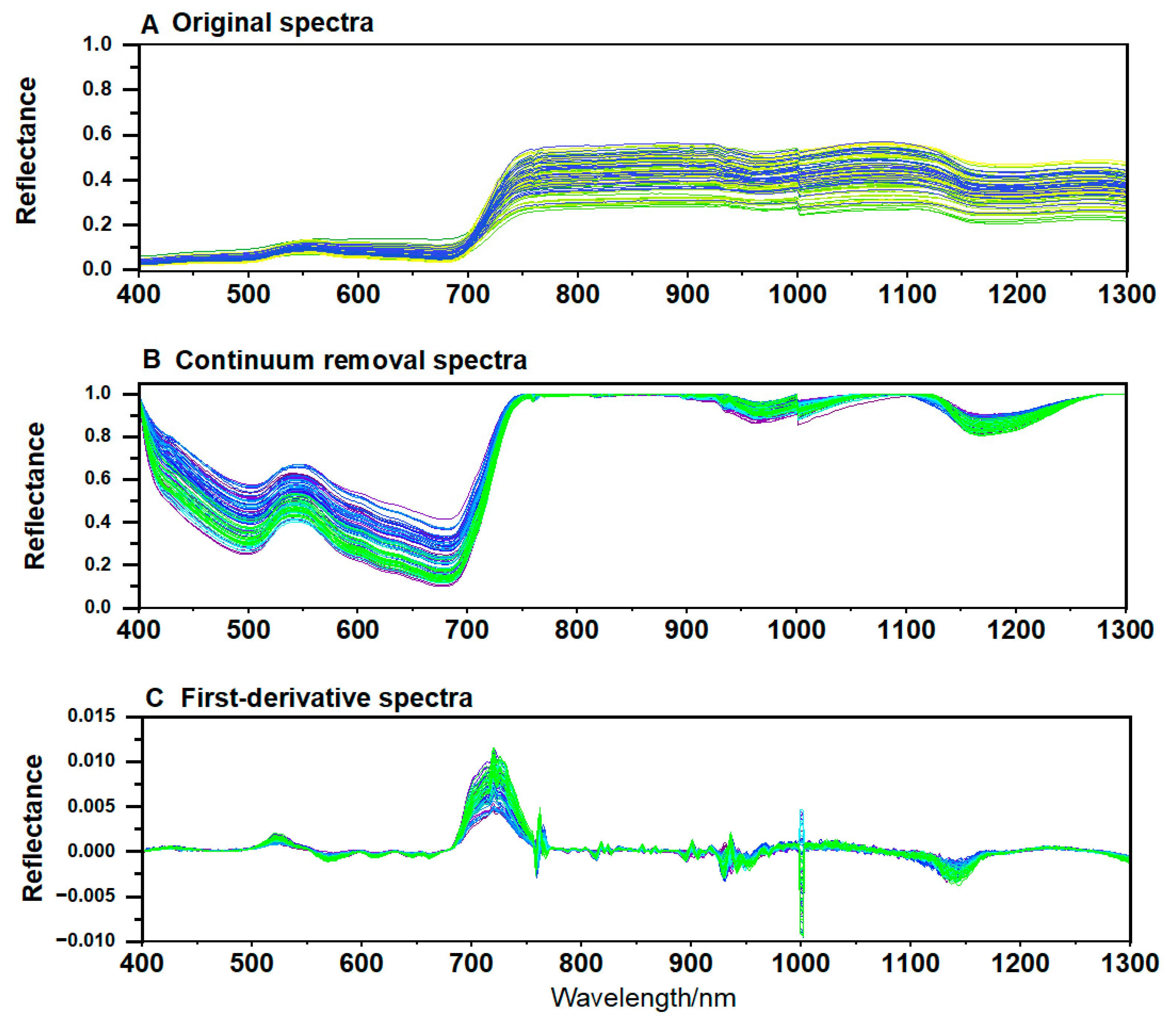
OS, CRS and FDS of the wolfberry tree canopy are presented in Figure 2, and the spectral changes resulting from different transformations are compared and analyzed. the variation characteristics of the original spectral reflectance of the wolfberry trees aligned with those of typical green plants, with the red edge feature being particularly prominent. In the visible light (VIS) wavelength range (400–680 nm) of the OS, two distinct regions of low reflectance are observed near the blue (400–480 nm) and red (600–680 nm) wavelengths, while minor reflection peaks occur around the green wavelength. The spectral reflectance remains below 20%, and the contrast between peaks and valleys is relatively weak in the VIS range. In the red edge region (680–750 nm), the spectral reflectance increases sharply, reaching a maximum value of approximately 60%. In the near-infrared (NIR) range (750–1300 nm), the reflectance is generally high, with water absorption features identified near 970 nm and 1200 nm.
CRS and OS exhibit similar trends; however, the gradient of waveform changes is more pronounced in CRS, leading to enhanced contrast between the depth of absorption valleys and the height of reflection peaks. This feature is particularly evident in the VIS range, where the red edge slope becomes steeper. Furthermore, the peak-to-valley contrast of CRS is still significant compared to FDS. However, it is noteworthy that the number of reflection peaks and absorption valleys in CRS is fewer than that in FDS.
After the first-derivative transformation, the slope of the red edge disappears and is replaced by a significant reflection peak, and the spectral curve exhibits distinct fluctuations with numerous small peaks and valleys, distinguishing it from both OS and CRS. Outside the red edge region, FDS shows similar reflectance values in both the VIS and NIR wavelength ranges, ranging from −0.0025 to 0.0025.

3.2. Correlation Analysis Between Spectra Variables and Nitrogen Content

3.2.1. Correlation Between Spectral Wavelengths and Nitrogen Content

A correlation analysis was conducted between the OS, FDS, and CRS with nitrogen content, and the distribution of correlation coefficients is illustrated in Figure 3. In general, when considering the coefficient distribution trend in the range of 400–1300 nm, the correlation coefficients for the OS and CRS were similar (i.e., the visible light bands all show negative correlation, while some of the near-infrared bands show positive correlation), while the correlation coefficients of the FDS fluctuate significantly.
In the OS, all wavelengths except for those at 735–955 nm and 1119–1134 nm exhibited a negative correlation with nitrogen content. Within the NIR range, the correlation coefficients were minimal and showed no correlation with nitrogen content. Conversely, in the red edge region, wavelengths at 709 nm, 710 nm, and 711 nm displayed weak correlation with nitrogen content, meeting only the significance threshold of p < 0.1. In the VIS region, wavelengths around 700 nm and 500 nm demonstrated strong correlations with nitrogen content, passing the p < 0.05 significance test. Additionally, all other visible light wavelengths (a total of 267) were statistically significant at the p < 0.01 level, with correlation coefficients ranging from −0.411 to −0.264.
In the VIS and red-edge regions, CRS revealed a negative correlation with nitrogen content, with nearly all wavelengths (a total of 355) exhibiting significant correlations with nitrogen content at the p < 0.01 level—correlation coefficients ranged from −0.354 to −0.286. In the NIR band, the correlation coefficients exhibited considerable variability, ranging from −0.512 to 0.522. Within this region, a total of 108 wavelengths were significantly correlated with nitrogen content at the p < 0.01 level, and they were mainly distributed around 750 nm, 800 nm, 1105–1115 nm, and 1256–1283 nm. Although the number of bands passing the p < 0.01 significance test was greater in the VIS region than in the NIR region, the strength of correlation was lower compared to that in the NIR region.
The relationship between FDS and nitrogen content exhibits considerable variability across different wavelengths. In the VIS region, there are 100 wavelengths that meet the threshold of p < 0.01, with correlation coefficients ranging from −0.454 to −0.265. In contrast, within the NIR region, there are 120 wavelengths exhibiting correlation coefficients between −0.577 and 0.488. This indicates that correlations in the NIR are stronger than those found in the VIS, which is similar to the CRS.
In summary, through correlation analysis, the initial 901 bands were reduced to 267 for the OS, 463 for the CRS, and 220 spectral windows for the FDS to further screen the characteristic spectral variables used for modelling. Moreover, based on the correlation coefficients, both the CRS and the FDS show improvement compared to the OS, especially in the NIR band.

3.2.2. Correlation Between PVIs and Nitrogen Content

The correlation between the PVIs and nitrogen content was evaluated using Spearman’s rank correlation (Table 4). The analysis revealed that RVI (D705,D722) (rs = −0.041, p > 0.05) and RVI (D730 D706) (rs = 0.158, p > 0.05) showed negligible correlations and were not statistically significant. In contrast, DD(rs = 0.202), NPCI(rs = 0.205), and CCI (rs = 0.223) demonstrated significant but weak correlations (p < 0.05). Furthermore, all 23 remaining vegetation indices demonstrated statistically significant correlations, exceeding our pre-specified screening threshold (p < 0.01) for feature selection. Among them, the strongest correlation was identified between PRI and nitrogen content, with a correlation coefficient of −0.367. Notably, the significance of weak correlations reflects the high statistical power of Spearman’s test with our sample size (n = 95) rather than model overfitting.

3.2.3. Correlation Between Ratio Spectral Index and Nitrogen Content

Figure 4 presents a heat map of correlation coefficients between the RSI and nitrogen content. By counting the number of RSI that passed the significance test at p < 0.01, we found that among the RSI-OS, a total of 32 passed the significance test at the 0.01 level, with correlation coefficients ranging from −0.377 to 0.345. Meanwhile, RSI-CRS and RSI-FDS had 38 and 20 significant RSI, respectively, with correlation coefficients ranging from −0.525 to 0.497 and from −0.456 to 0.388.
Clearly, RSI-CRS outperformed RSI-OS and RSI-FDS in both the number of RSI passing the significance test at the 0.01 level and the strength of correlation. Specifically, RSI808/1280 exhibited the strongest negative correlation with nitrogen content, with a correlation coefficient of −0.525. It is worth noting that although the number of RSI passing the 0.01 significance test in FDS is fewer than that in OS, their correlation coefficients with nitrogen content are stronger than those of OS.

3.3. Feature Spectral Variables Selection

Figure 5 shows the variable importance of spectral features. The results indicate that in the OS, the spectral wavelengths with high feature importance scores are primarily concentrated around 400 nm, 520 nm, 560 nm, and 690 nm in the VIS region. In the CRS, the wavelengths near 800 nm, 1100 nm, and 1280 nm in the NIR region exhibit high scores. As for the FDS, the wavelengths with high scores are distributed around 780 nm, 870 nm, 1100 nm, and 1250 nm in the NIR region, which is similar to the distribution observed in the CRS.
As depicted in Figure 6, the selected feature variables from the PVIs encompass PRI, NDVI2, NDVIgb, NDRE, NRI, PPR, VOG1, GI, SR (550, 670), and RVI1. Most of them exhibit wavelengths that fall within the VIS range. For instance, the wavelengths of NDVIgb, PPR, and PRI are situated in the green and blue bands; those of SR (550–670), RVI1, GI, and NRI reside in the green and red-edge bands; while VOG1 and NDRE have their wavelengths located within the red-edge band. Notably, only one wavelength from NDVI2 is positioned in the NIR range.
For the RSI-OS feature variable set, all sensitive wavelengths selected from the original spectra (OS) are included, except for 675 nm and 702 nm. Similarly, for the RSI-CRS feature spectral variable set, all sensitive wavelengths selected from the continuum-removed spectra (CRS) are included, except for 1118 nm. Finally, for the RSI-FDS feature spectral variable set, all sensitive wavelengths selected from the first-derivative spectra (FDS) are included, except for 1112 nm. In summary, the feature indices selected from the ratio spectral indices did not include all the sensitive bands identified from the spectral dataset.

3.4. Multivariate Regression Model

3.4.1. Model Construction

Seven feature spectral variables were utilized as inputs to predict the nitrogen content in wolfberry canopy using various methods, including RF, AdaBoost, ExtraTrees, CatBoost, XGBoost, GDLR, OLSLR, and Ridge Regression (RR) (Figure 7). The main parameters of the model are shown in Table 5.
Analysis of the input feature variables showed that the R2 for models based on FDS ranged from 0.341 to 0.976, all exceeding those of OS-based models, which ranged from 0.107 to 0.897. Additionally, the RMSE values for FDS-based models varied between 0.061 and 0.307 while MAE values ranged from 0.026 to 0.223; both metrics were lower than those observed in OS-based models. The RMSE of OS-based models ranged from 0.143 to 0.361, and the MAE spanned from 0.058 to 0.274. For CRS-based models, except for the XGBoost model, the R2 of the other models ranged from 0.297 to 0.945, which were higher than those of the OS-based models. The RMSE and MAE values of the CRS-based models ranged from 0.084 to 0.317 and 0.049 to 0.224, respectively, which were lower than those of the OS-based models. This performance pattern is consistent with that exhibited by FDS-based models; thus, it can be concluded that both CRS- and FDS-based modelling approaches demonstrate superior performance compared to OS-based methodologies.
Compared to the models based on RSI-OS and PVIs, the models based on RSI-CRS and RSI-FDS demonstrate superior performance, as evidenced by their higher R2 and lower values for RMSE and MAE. The R2 for the RSI-CRS and RSI-FDS models ranged from 0.282 to 0.941 and 0.350 to 0.929, respectively, while their RMSE and MAE values ranged from 0.096 to 0.320 and 0.106 to 0.308, as well as from 0.041 to 0.230 and 0.048 to 0.230, respectively. In contrast, the R2 for the models utilizing RSI-PVIS ranged from 0.159 to 0.870, with corresponding RMSE and MAE values ranging from 0.128 to 0.349 and 0.068 to 0.319, respectively. Although the R2 for the AdaBoost model based on RSI-OS is marginally higher than that of both the RSI-CRS and RSI-FDS models, it is noteworthy that other models relying on RSI-OS exhibit lower R2 values compared to those derived from either RSI-CRS or RSI-FDS frameworks. Furthermore, their RMSE and MAE metrics are also higher than those associated with the latter two models. Overall, it is evident that the performance of both the RSI-CRS and RSI-FDS models surpasses that of their counterparts based on either RSI-OS or PVIs methodologies.
As shown in Figure 7, the R2 of the linear regression models—GDLR, OLSLR, and RR—are significantly lower than those of the nonlinear regression models, including RF, AdaBoost, ExtraTrees, CatBoost, and XGBoost. Additionally, the RMSE and MAE values of the linear regression models are considerably higher than those of the nonlinear regression models. Specifically, the R2 values for the linear regression models range from 0.107 to 0.669, with RMSE and MAE values ranging from 0.208 to 0.361 and 0.149 to 0.319, respectively. In contrast, the R2 values for the nonlinear regression models range from 0.768 to 0.976, with RMSE and MAE values ranging from 0.061 to 0.171 and 0.026 to 0.132, respectively. These results clearly demonstrate that the performance of all nonlinear regression models is significantly superior to that of the linear regression models.

3.4.2. Model Validation

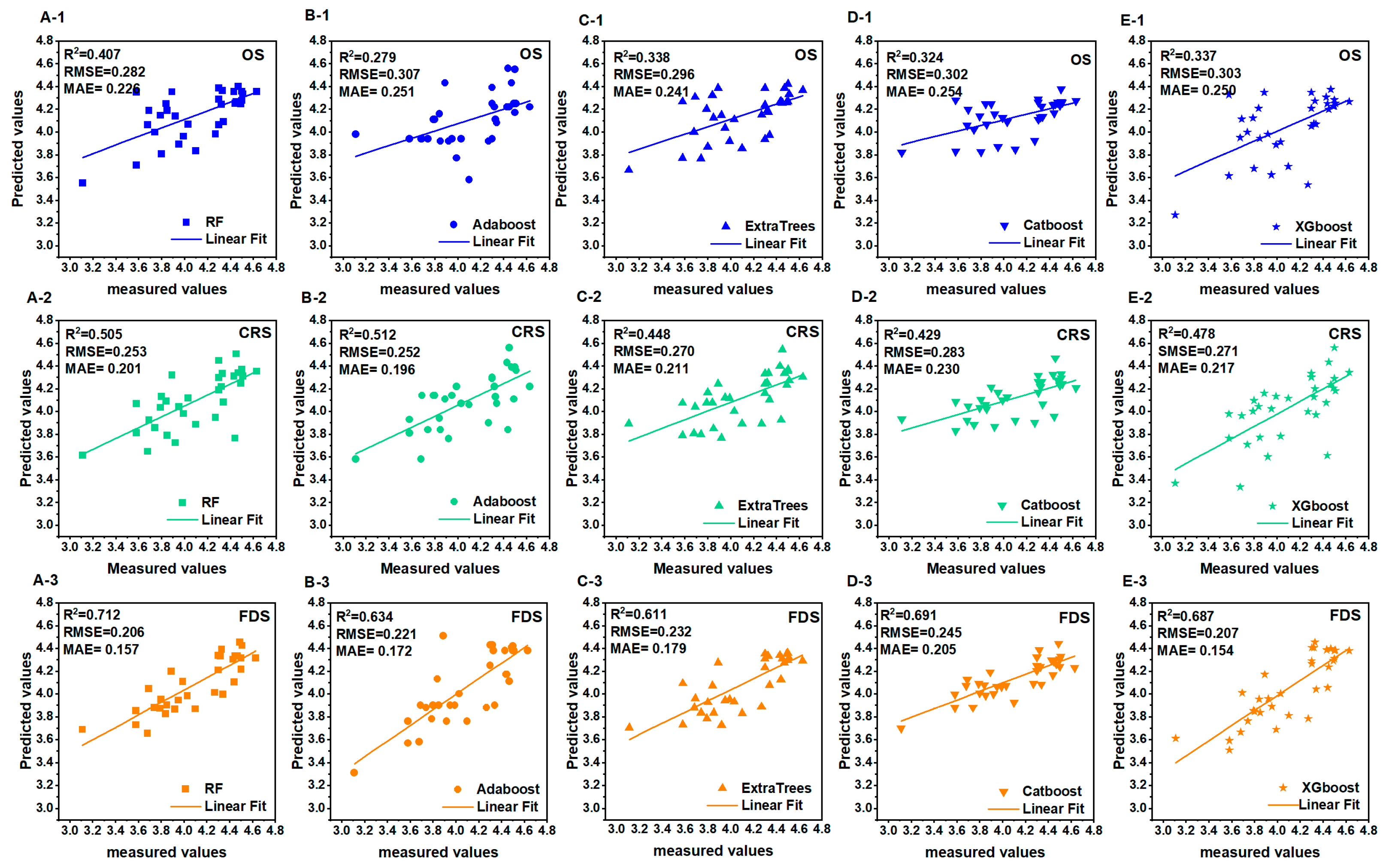
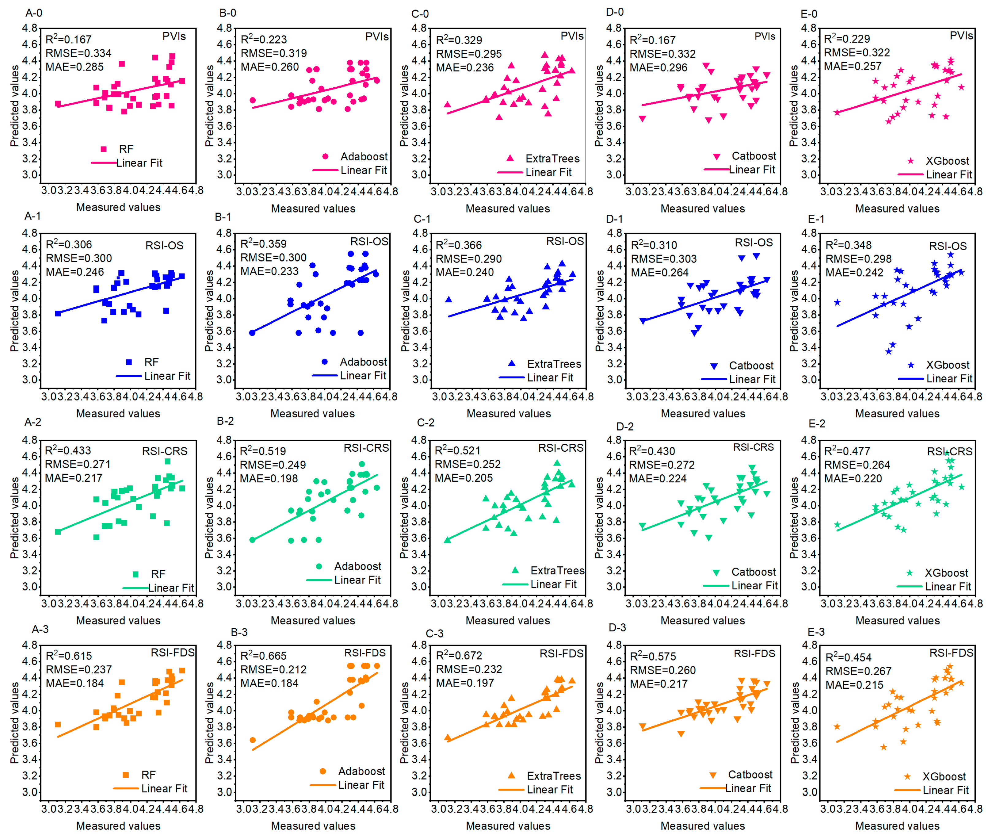
To explore the potential of spectral transformation combined with nonlinear regression methods for estimating nitrogen content in wolfberry canopies, the predictive performance of nonlinear regression models was evaluated using the test dataset (Figure 8 and Figure 9).
The performance of the models based on three types of sensitive wavelengths in estimating nitrogen content varied significantly (Figure 8). The OS-based models exhibited the weakest explanatory ability for nitrogen content, with R2 values of 0.279–0.407. The CRS-based models showed moderate performance, with R2 values of 0.429–0.512, while the FDS-based models demonstrated the strongest performance, with R2 values ranging from 0.611 to 0.712. These results indicate that the predictive ability of the CRS-based and FDS-based models was significantly improved compared to the OS-based models. Specifically, the RF model based on FDS exhibited the strongest explanatory power for nitrogen variation, with an R2 of 0.712, RMSE of 0.206, and MAE of 0.157.
The performance of the models based on four types of feature indices in estimating nitrogen content varied significantly (Figure 9). The PVIs-based models exhibited the weakest explanatory ability for nitrogen content, with R2 values of 0.167–0.329. The RSI-OS-based models showed slightly better performance, with R2 values of 0.306–0.366. The models based on RSI-CRS-based exhibited stronger performance, with R2 values of 0.430–0.521. The RSI-FDS-based models demonstrated the best performance, with R2 values of 0.454–0.672. These results indicate that using PVIs to predict nitrogen content in wolfberry canopies is not feasible. By comparison, the predictive ability of the RSI-CRS-based and RSI-FDS-based models was significantly improved compared to the RSI-OS-based models. Specifically, the ExtraTrees model based on RSI-FDS exhibited the highest prediction ability, with an R2 of 0.672, RMSE value of 0.232, and MAE value of 0.197.
Analysis of the models presented in Figure 8 and Figure 9 revealed a clear ranking in terms of their R2 values. The PIVs-based models exhibited the lowest R2 values, ranking first. OS-based and RSI-OS models were closely related, sharing the second rank. CRS-based models followed in third place, while RSI-CRS-based models ranked fourth. RSI-FDS-based models came in fifth, and FDS-based models had the highest R2 values, ranking last. This sequence indicates that first-derivative and continuum removal transformation significantly enhance the predictive performance for nitrogen content in wolfberry canopies, with the first-derivative transformation showing the greatest improvement.

3.4.3. Model Accuracy Comparison

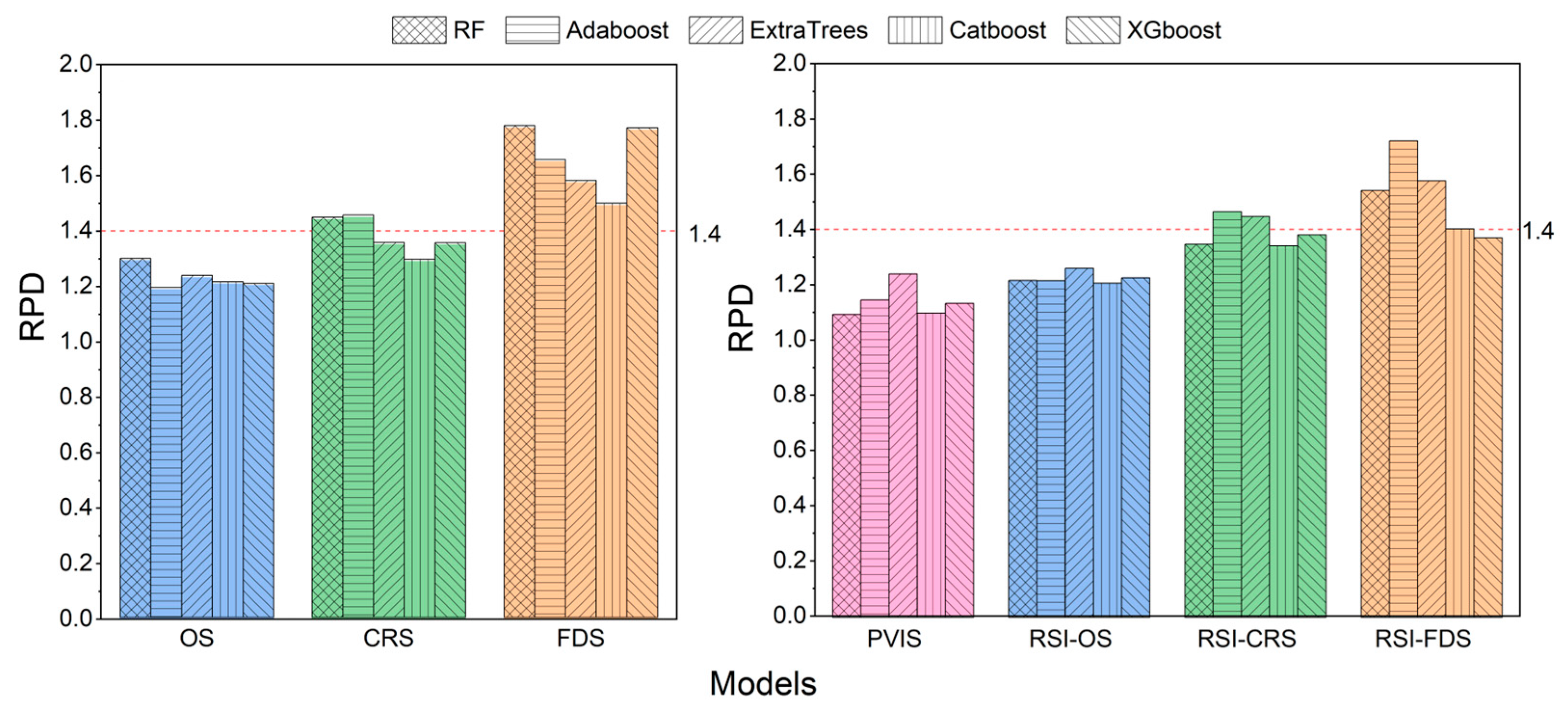
As can be seen in Figure 10, among the five models (RF, AdaBoost, ExtraTrees, CatBoost, and XGBoost), all PVIs-based models exhibited the lowest RPD values. Although the PVIs-based ExtraTrees model had the highest RPD value among these models, it was only 1.238, and its R2 value on the test dataset was also only 0.330.
When using OS, although the RPD values of both OS-based and RSI-OS-based models exceeded those of PVIs-based models, all values remained below 1.4. Specifically, in OS-based models, the maximum RPD value was only 1.293, with an R2 value of 0.407 for the validation set. Similarly, in RSI-OS-based models, the highest RPD value was only 1.259, with an R2 value of 0.365 for the validation set. These results indicate that neither PVIs-based models nor models based on OS feature variables (sensitive wavelengths and ratio spectral indices) are reliable for predicting nitrogen content in wolfberry canopy.
In the continuum-removal transform spectra, the RF and AdaBoost models based on CRS sensitive wavelengths, along with the Adaboost and ExtraTrees models based on RSI-CRS, achieved RPD values of 1.441, 1.448, 1.464, and 1.446, respectively, all exceeding the threshold of 1.4. The corresponding R2 for the test dataset were 0.505, 0.512, 0.519, and 0.521. These results indicate that the four continuum-removal-based models exhibit moderate explanatory power for predicting nitrogen content in the wolfberry canopy. They only account for slightly over 50% of the variation in nitrogen content.
In the first-derivative transform spectra, all multivariate nonlinear regression models based on FDS sensitive wavelengths achieved RPD values exceeding the threshold of 1.4. Similarly, all models based on RSI-FDS, except for the XGboost model, also surpassed this threshold. Specifically, the CatBoost models based on RSI-FDS and FDS demonstrated RPD values of 1.492 and 1.401, respectively. The ExtraTrees model based on FDS, the RF model based on RSI-FDS, and the ExtraTrees model based on RSI-FDS achieved RPD values of 1.574, 1.539, and 1.575, respectively. The AdaBoost model based on FDS recorded an RPD of 1.650, while the AdaBoost, XGBoost, and RF models based on FDS achieved RPD values of 1.718, 1.764, and 1.772, respectively. These findings highlight that the combination of first-derivative transformation and nonlinear regression methods offers high prediction accuracy for nitrogen content in wolfberry canopy. Notably, the RF model based on FDS delivered the best performance, with an RPD of 1.772, a modelling set R2 of 0.914, and a test set R2 of 0.712.

4. Discussion

Accurate monitoring of canopy nitrogen content is critical for optimizing fertilization management in wolfberry cultivation, and hyperspectral remote sensing offers a promising non-destructive approach. This study integrated spectral transformations, feature selection, and multivariate regression models to explore the potential of canopy hyperspectral data for nitrogen estimation in wolfberry, with key findings providing insights into both methodological and practical implications.

4.1. Selection of the Research Spectral Range

Canopy spectra can effectively reflect the overall nitrogen status of plants [12]. In the field of agricultural remote sensing, analyzing canopy spectral reflectance to assess crop nitrogen status is a critical focus area [59]. Precise monitoring of canopy nitrogen status through canopy spectral reflectance primarily relies on the response of crop leaf biophysical components to canopy spectral reflectance [60]. Spectral reflectance of canopies across different wavelength ranges reflects distinct characteristics of ground objects. The wavelengths sensitive to fresh leaf nitrogen content are primarily located in the NIR plateau and the VIS region. Previous studies on the screening of nitrogen-sensitive wavelengths and the estimation of nitrogen content in rice have demonstrated that nitrogen inversion wavelengths at the canopy scale are predominantly distributed within the 400–900 nm range, with only a few scattered wavelengths in the vicinity of 950–1200 nm and 2100 nm [12]. Research by Fu et al. also indicates that the nitrogen status in crop leaves can be estimated using visible and near-infrared bands [61]. Additionally, studies by He et al. and Wan et al. have shown that near-infrared reflectance is less sensitive to sunlight and shadows, making it advantageous for nitrogen estimation [62,63]. Shu et al. further demonstrated that incorporating near-infrared reflectance data significantly enhances the accuracy of nitrogen estimation [25].
The shortwave infrared range (1300–2500 nm) contains two strong water absorption regions (around 1450 nm and 1940 nm) [64], where intense water absorption often masks nitrogen absorption features. This complicates the relationship between shortwave infrared reflectance and nitrogen content, making it challenging for nitrogen diagnosis under standard field conditions. However, studies have demonstrated that with advanced correction techniques, meaningful nitrogen-related signals can still be extracted from these longer wavelengths in certain contexts [5]. This capability arises because changes in the shortwave infrared spectrum are driven by moisture, dry matter, protein, and cellulose content, and protein content is closely linked to leaf nitrogen content. Therefore, leaf nitrogen content can be characterized by shortwave infrared reflectance [65,66]. Methods such as Competitive Adaptive Reweighted Sampling (CARS), Successive Projection Algorithm (SPA), and Random Frog Algorithm can extract nitrogen-sensitive spectral features from the shortwave infrared band of apple canopy spectra [57]. These approaches represent a viable pathway for future research.
Our decision to exclude SWIR bands prioritized developing a parsimonious field monitoring tool for wolfberry, emphasizing practicality over extended spectral coverage. Additionally, comparative analysis of wolfberry canopy reflectance revealed exceptionally high noise levels in the 350–400 nm and 2400–2500 nm wavelength ranges. Despite implementing mathematical transformations for noise reduction, results remained unsatisfactory, rendering these spectral regions ineffective for nitrogen monitoring. Consequently, these bands were excluded from further analysis, yielding a refined effective range of 400–1300 nm encompassing 901 sampled wavelengths. Notably, feature wavelengths selected from CRS and FDS in this study are predominantly concentrated in the NIR region, and the models developed based on these NIR feature wavelengths exhibit strong performance in estimating nitrogen content in wolfberry canopy, which aligns with the conclusions of previous studies [25,62,63].

4.2. Application of Mathematical Transformations

The application of mathematical transformation methods to spectral data can reduce noise, enhance spectral features, and improve the accuracy of predictive models [67]. Continuum removal transformation mitigates the influence of background spectra and effectively highlights the absorption and reflection characteristics of spectral curves [68]. Differential transformation partially eliminates the effects of atmospheric conditions, shadows, and soil—factors related to the vegetation environment—on the baseline, while capturing abrupt changes in the spectrum [7]. Research by Tang et al. has demonstrated that first-derivative transformation can effectively decompose the red-edge spectrum and enhance the characteristics of the red-edge band [11].
In this study, after applying continuum removal transformation to the original spectra, the differences in the VIS band were significantly enhanced. Following the first-derivative transformation, the red-edge spectrum was effectively decomposed. The maximum absolute values of the correlation coefficients between continuum-removed spectra and nitrogen content increased by 27%, while those between first-derivative spectra and nitrogen content increased by 43%, compared with those of the original spectra. Consequently, both spectral transformations improved the relationship between spectral variables and nitrogen content to some extent. Models constructed based on these two transformed spectra outperformed those based on the original spectra, with the maximum R2 in the validation sets increasing by 26.8% and 73.2%, respectively. This indicates that mathematical transformations positively impact the estimation of nitrogen content in the wolfberry canopy. Both continuum removal and first-derivative transformations achieved strong results in this study. Similar conclusions were reported by Arkin Ansarin et al., who used continuum removal and first-derivative transformations to estimate chlorophyll content in long-staple cotton leaves via hyperspectral techniques [69].

4.3. Feature Spectral Variable Screening

Hyperspectral remote sensing, with its high spectral resolution and continuous band coverage, enables precise nitrogen status diagnosis for specific crops. However, the high dimensionality of hyperspectral data poses significant challenges in developing robust estimation models, as not all spectral bands contribute equally to crop nitrogen assessment. Previous studies have demonstrated that incorporating all spectral bands in nitrogen estimation models may introduce noise and increase the risk of overfitting, consequently compromising model predictive accuracy. Feature selection through spectral band reduction has been shown to mitigate overfitting while enhancing regression model performance [55].
In this study, we implemented a hybrid approach integrating correlation analysis with Recursive Feature Elimination (RFE) for optimal spectral feature selection. This methodology effectively reduced dimensionality while preserving biochemically relevant spectral variables, enhancing model robustness. For FDS and CRS transformations, selected features were predominantly concentrated in the near-infrared (NIR) region—consistent with established literature demonstrating NIR reflectance’s lower sensitivity to environmental noise (e.g., solar angle variations) and stronger association with foliar biochemistry [25,62,63]. Conversely, OS-derived features were dominated by visible bands exhibiting weaker correlations, highlighting the critical role of spectral transformations in extracting meaningful biological signals. Validation performance confirmed this advantage: CRS and FDS models achieved maximum R2 values of 0.512 and 0.712, respectively, significantly surpassing the OS model’s 0.407. Furthermore, ratio spectral indices (RSI) derived from transformed spectra (RSI-FDS, RSI-CRS) outperformed published vegetation indices (PVIs), with RSI-FDS models attaining validation R2 up to 0.672 (Section 3.4.2). This demonstrates that data-driven indices tailored to wolfberry’s unique spectral characteristics provide superior predictive capability compared to generalized PVIs developed for other crops.

4.4. Superiority of Nonlinear Machine Learning Models

Our results demonstrate the clear superiority of nonlinear machine learning models (RF, AdaBoost, ExtraTrees, CatBoost, XGBoost) over linear regression approaches (GDLR, OLSLR, RR) for predicting wolfberry nitrogen content. Nonlinear models achieved training R2 values of 0.768–0.976, significantly outperforming linear models (0.107–0.669). This substantial performance gap originates from inherent complexities in wolfberry canopy systems. As a perennial shrub with continuous flowering and fruiting, wolfberry develops heterogeneous canopies where leaves, branches, flowers, and fruits behaviour coexist [31]. This architectural complexity, combined with low canopy coverage in arid/semi-arid environments [2], generates nonlinear spectral interactions. Even when targeting dense leaf clusters, residual influences from soil background reflectance and environmental variables (e.g., solar geometry variations, dust) introduce non-additive noise that violates linear assumptions. This results in a strong non—linear relationship between the spectral characteristics of the wolfberry canopy and the nitrogen content. Nonlinear models employing ensemble learning techniques are better equipped to handle high-dimensional spectral data and decode these complexities [13,21]. In contrast, linear models are fundamentally constrained by their assumption of additive relationships, which restricts their ability to capture the non—linear relationships between nitrogen and spectra. Our results align with previous studies demonstrating the superior performance of machine learning over traditional regression analysis in estimating biophysical parameters from hyperspectral data.
While all nonlinear models outperformed linear methods, the Random Forest (RF) model utilizing feature wavelengths derived from first-derivative spectra demonstrated optimal performance. This model achieved training and validation R2 values of 0.914 and 0.712, respectively, with a Residual Prediction Deviation (RPD) of 1.772. RF’s superiority over other ensemble methods stems from its algorithmic alignment with dataset characteristics: dual randomization mechanisms (Bootstrap resampling and random feature selection) effectively suppress spectral noise while providing implicit data augmentation under small-sample conditions (n = 95). The multi-tree decision strategy comprehensively captures complex nonlinear responses between nitrogen content and near-infrared (NIR) bands (750–1300 nm), with default parameters exhibiting high inherent robustness. In contrast, AdaBoost amplifies measurement errors through noise weight accumulation during iterative boosting, XGBoost/CatBoost exhibit unstable gradient optimization due to sample constraints, and ExtraTrees diminishes key wavelength contributions through excessive randomization of splits.

4.5. Comparison with Existing Literature and Study Significance

Most prior studies on spectral nitrogen estimation focus on annual crops (e.g., rice [12], wheat [13,21], and maize [25]) or select fruit trees (e.g., apple [6], litchi [27]), with limited research on perennial shrubs like wolfberry. Our study addresses this gap by demonstrating that hyperspectral techniques, when integrated with FD transformation and RF modelling, can reliably estimate wolfberry canopy nitrogen (RPD = 1.772, approaching the “excellent” prediction threshold defined by [52]). Compared with the studies on lychees [27] and apples [6]—where the reported nitrogen estimation validation R2 values are less than 0.8— our RF-FDS model achieves comparable accuracy while offering a more practical framework: integrating: (1) canopy spectral measurement, (2) first-derivative spectral transformation, (3) hybrid feature selection combining correlation and RFE, and (4) random forest regression. Crucially, this framework utilizes a ground-based portable spectrometer for on-site monitoring, circumventing the costs and operational complexities of aerial or satellite platforms. This approach is particularly suitable for smallholder farms in Ningxia, the primary global wolfberry-producing region.

4.6. Future Perspectives

Despite the promising results of using hyperspectral remote sensing combined with machine learning for estimating wolfberry canopy nitrogen content, several directions to enhance practical applicability and expand research depth warrant further exploration:
The current optimal model (Random Forest based on first-derivative spectra) was validated primarily in the arid and semi-arid regions of Ningxia, with a focus on the summer flowering and fruiting stage. To improve its universality, future research should extend validation to other major wolfberry-growing regions (e.g., Xinjiang, Qinghai), which feature diverse soil types, microclimates, and cultivars beyond “Ningqi No. 7.” Notably, such expansion should include systematic calibration for regional differences—for example, adjusting for soil background interference in high-salinity areas of Xinjiang or light intensity variations in Qinghai’s plateau environments. Incorporating multi-region datasets will refine the model’s generalization capability, ensuring stable performance across complex field scenarios.
Additionally, nitrogen dynamics in wolfberries vary significantly across phenological stages. Expanding the model to cover the entire growth cycle—particularly critical periods such as sprouting (early April) and autumn fruiting (mid-August to September)—will improve its temporal adaptability and enable dynamic tracking of nitrogen demand. This temporal extension would support seasonal fertilization management, aligning nutrient supply with crop growth stages to achieve more precise and efficient fertilization.
Overall, advancing these research directions will strengthen the robustness and practicality of the hyperspectral-based nitrogen monitoring framework, facilitating its broader application in wolfberry cultivation. By bridging regional and temporal limitations, the model can better support sustainable agricultural practices and provide references for optimizing fertilizer use across diverse growing conditions.

5. Conclusions

This study proposes an integrated framework combining canopy spectral measurements, spectral mathematical transformations, feature variable selection, and machine learning modelling. The research highlights the potential of hyperspectral remote sensing integrated with mathematical transformations and machine learning algorithms for accurate and rapid nitrogen content estimation. Results demonstrate that spectral transformations significantly enhance spectral-nitrogen relationships, thereby improving model performance. Compared with original spectra, the maximum absolute correlation coefficients between nitrogen content and continuum-removed spectra, as well as first-derivative spectra, increased by 27.0% and 40.4%, respectively, while validation set R2 values improved by 27.96% and 74.88%. Machine learning-based nonlinear models outperformed conventional linear regression models, indicating a strong nonlinear relationship between spectral features and nitrogen content. Specifically, the Random Forest (RF) model trained on first-derivative spectra (FDS) achieved the highest accuracy, with R2 values of 0.914 for the training set and 0.712 for the validation set, and a ratio of performance to deviation (RPD) of 1.772, highlighting the efficacy of this integrated methodology. However, it is important to emphasize that the current validation was conducted solely within the arid/semi-arid region of Ningxia during the summer flowering and fruiting stage. While the proposed framework exhibits strong potential for operational field monitoring of wolfberry nitrogen status, its broader applicability and immediate operational deployment require rigorous validation across diverse geographical regions (e.g., Xinjiang, Qinghai) featuring different soil types, microclimates, and cultivars, as well as across the entire phenological cycle (as detailed in Section 4.6). Successfully addressing these validation needs will be crucial to unlock the full potential of this approach for enabling dynamic, precision nitrogen management in diverse wolfberry production systems.

Author Contributions

Conceptualization, H.W. and H.Z.; methodology, H.Z. and Y.L.; software, Y.L. and L.Z.; validation, Y.L. and L.Z.; formal analysis, W.X. and Y.L.; investigation, Y.L., L.Z. and W.X.; writing—original draft preparation, Y.L.; writing—review and editing, Y.L., L.Z. and H.Z.; visualization, Y.L.; supervision, H.W.; project administration, Y.L.; funding acquisition, Y.L. All authors have read and agreed to the published version of the manuscript.

Funding

This research was funded by the Ningxia Natural Science Fund of China, funding number 2023AAC02054, 2022AAC03432 and 2020AAC03294.

Data Availability Statement

Data are contained within the article.

Conflicts of Interest

Author Ligen Zhang was employed by the company Ningxia Academy of Building Research Co., Ltd. The remaining authors declare that the research was conducted in the absence of any commercial or financial relationships that could be construed as a potential conflict of interest.

Abbreviations

RFERecursive Feature Elimination
OSoriginal spectra
CRScontinuum-removed spectra
FDSfirst-derivative spectra
PVIspublished vegetation indices
RSIratio spectral index
RSI-OSratio spectral indices from original spectra
RSI-CRSratio spectral indices from continuum-removed spectra
RSI-FDSratio spectral indices from first-derivative spectra

References

  1. Ma, Y.P.; Wang, Z.J.; Li, Y.M.; Feng, X.R.; Song, L.H.; Gao, H.D.; Cao, B. Fruit morphological and nutritional quality features of goji berry (Lycium barbarum L.) during fruit development. Sci. Hortic. 2023, 308, 111555. [Google Scholar] [CrossRef]
  2. Yin, Z.R.; Huang, J.C.; Gui, L.G.; Zhao, Y.; Lei, J.Y. Characteristics of soil water movement in wolfberry fields under different drip irrigation amounts. Acta Agric. Boreali-Occident. Sin. 2020, 29, 1695–1702. [Google Scholar]
  3. Deng, Z.; Yin, J.; Eeswaran, R.; Gunaratnam, A.; Wu, J.; Zhang, H. Interacting effects of water and compound fertilizer on the resource use efficiencies and fruit yield of drip-fertigated Chinese wolfberry (Lycium barbar. L.). Technol. Hortic. 2024, 4, e019. [Google Scholar] [CrossRef]
  4. Li, L.; Li, F.; Liu, A.Y.; Wang, X.Y. The prediction model of nitrogen nutrition in cotton canopy leaves based on hyperspectral visible-near infrared band feature fusion. Biotechnol. J. 2023, 18, e2200623. [Google Scholar] [CrossRef]
  5. Peanusaha, S.; Pourreza, A.; Kamiya, Y.; Fidelibus, M.W.; Chakraborty, M. Nitrogen retrieval in grapevine (Vitis vinifera L.) leaves by hyperspectral sensing. Remote Sens. Environ. 2024, 302, 113966. [Google Scholar] [CrossRef]
  6. Han, M.X.; Zhang, L. Effects of fertilization methods and nitrogen content application on soil water and nitrogen distribution under microporous ceramic root irrigation of Lycium barbarum. Water Sav. Irrig. 2021, 1, 60–64. [Google Scholar]
  7. Li, M.X.; Zhu, X.C.; Li, W.; Tang, X.Y.; Yu, X.Y.; Jiang, Y.M. Retrieval of nitrogen content in apple canopy based on unmanned aerial vehicle hyperspectral images using a modified correlation coefficient method. Sustainability 2022, 14, 1992. [Google Scholar] [CrossRef]
  8. Shivashankar, K.; Potdar, P.M.; Gawdiya, S.; Golshetti, A.; Kanade, A.K.; Balol, G.; Biradar, D.P.; Math, K.K.; Al-Ansari, N.; El-Hendawy, S.; et al. SPAD dynamics in maize crop with precision nitrogen management under rain-fed and irrigated conditions. Sci. Rep. 2025, 15, 22842. [Google Scholar] [CrossRef] [PubMed]
  9. Yang, J.; Jiang, J.; Fu, Z.; Wang, W.; Cao, Q.; Tian, Y.; Zhu, Y.; Cao, W.; Liu, X. Integrating phenology information with UAV multispectral data for rice nitrogen nutrition diagnosis. Eur. J. Agron. 2025, 169, 127696. [Google Scholar] [CrossRef]
  10. Ghazal, S.; Kommineni, N.; Munir, A. Comparative Analysis of Machine Learning Techniques Using RGB Imaging for Nitrogen Stress Detection in Maize. AI 2024, 5, 1286–1300. [Google Scholar] [CrossRef]
  11. Tang, Z.J.; Wang, X.; Xiang, Y.Z.; Liang, J.P.; Guo, J.J.; Li, W.Y.; Lu, J.S.; Du, R.Q.; Li, Z.J.; Zhang, F.C. Application of hyperspectral technology for leaf function monitoring and nitrogen nutrient diagnosis in soybean (Glycine max L.) production systems on the Loess Plateau of China. Eur. J. Agron. 2024, 154, 127098. [Google Scholar] [CrossRef]
  12. Wang, J.J.; Song, X.Y.; Mei, X.; Yang, G.J.; Li, Z.H.; Li, H.L.; Meng, Y. Sensitive bands selection and nitrogen content monitoring of rice based on Gaussian regression analysis. Spectrosc. Spectr. Anal. 2021, 41, 1722–1729. [Google Scholar]
  13. Fan, K.; Li, F.L.; Chen, X.K.; Li, Z.F.; Mulla David, J. Nitrogen balance index prediction of winter wheat by canopy hyperspectral transformation and machine learning. Remote Sens. 2022, 14, 3504. [Google Scholar] [CrossRef]
  14. Peng, Y.F.; Zhu, X.C.; Xiong, J.L.; Yu, R.Y.; Liu, T.L.; Jiang, Y.M.; Yang, G.J. Estimation of nitrogen content on apple tree canopy through red-edge parameters from fractional-order differential operators using hyperspectral reflectance. J. Indian Soc. Remote Sens. 2020, 49, 377–392. [Google Scholar] [CrossRef]
  15. Yu, F.H.; Bai, J.C.; Jin, Z.Y.; Zhang, H.G.; Yang, J.X.; Xu, T.Y. Estimating the rice nitrogen nutrition index based on hyperspectral transform technology. Front. Plant Sci. 2023, 14, 1118098. [Google Scholar] [CrossRef]
  16. Peng, Z.G.; Lin, S.Z.; Zhang, B.Z.; Wei, Z.; Liu, L.; Han, N.N.; Cai, J.B.; Chen, H. Winter Wheat Canopy Water Content Monitoring Based on Spectral Transforms and “Three-edge” Parameters. Agric. Water Manag. 2020, 240, 106306. [Google Scholar] [CrossRef]
  17. Zhou, X.T.; Yang, M.; Chen, X.Y.; Ma, L.L.; Yin, C.X.; Qin, S.Z.; Wang, L.; Lv, X.; Zhang, Z. Estimation of cotton nitrogen content based on multi-angle hyperspectral data and machine learning models. Remote Sens. 2023, 15, 955. [Google Scholar] [CrossRef]
  18. Song, X.; Xu, D.Y.; Huang, S.M.; Huang, C.C.; Zhang, S.Q.; Guo, D.D.; Zhang, K.K.; Yue, K. Nitrogen content inversion of wheat canopy leaf based on ground spectral reflectance data. J. Appl. Ecol. 2020, 31, 1636–1644. [Google Scholar]
  19. Li, H.; Li, D.; Xu, K.; Cao, W.; Jiang, X.; Ni, J. Monitoring of Nitrogen Indices in Wheat Leaves Based on the Integration of Spectral and Canopy Structure Information. Agronomy 2022, 12, 833. [Google Scholar] [CrossRef]
  20. Verrelst, J.; Camps-Valls, G.; Muñoz-Marí, J.; Rivera, J.P.; Veroustraete, F.; Clevers, J.G.P.W.; Moreno, J. Optical remote sensing and the retrieval of terrestrial vegetation bio-geophysical properties—A review. ISPRS J. Photogramm. Remote Sens. 2025, 108, 273–290. [Google Scholar] [CrossRef]
  21. Sahoo, R.N.; Rejith, R.G.; Gakhar, S.; Ranjan, R.; Meena, M.C.; Dey, A.; Mukherjee, J.; Dhakar, R.; Meena, A.; Daas, A.; et al. Drone remote sensing of wheat N using hyperspectral sensor and machine learning. Precis. Agric. 2023, 25, 704–728. [Google Scholar] [CrossRef]
  22. Yang, F.Q.; Dai, H.Y.; Feng, H.K.; Yang, G.J.; Li, Z.H.; Chen, Z.X. Hyperspectral estimation of plant nitrogen content based on Akaike’s information criterion. Trans. Chin. Soc. Agric. Eng. 2016, 32, 161–167. [Google Scholar]
  23. Feng, J.; Lu, Z.Y.; Ma, X.Y.; Chen, S.L.; Zhao, Q.H.; Wang, S.W. Crop canopy nitrogen inversion based on hyperspectral corn field geese model. J. Agric. Mech. Res. 2020, 42, 4–11. [Google Scholar]
  24. Wen, P.F.; Shi, Z.J.; Li, A.; Ning, F.; Zhang, Y.H.; Wang, R.; Li, J. Estimation of the vertically integrated leaf nitrogen content in maize using canopy hyperspectral red edge parameters. Precis. Agric. 2020, 22, 984–1005. [Google Scholar] [CrossRef]
  25. Shu, M.Y.; Zhu, J.Y.; Yang, X.H.; Gu, X.H.; Li, B.G.; Ma, Y.T. A spectral decomposition method for estimating the leaf nitrogen status of maize by UAV-based hyperspectral imaging. Comput. Electron. Agric. 2023, 212, 108100. [Google Scholar] [CrossRef]
  26. Alfadhl, A.; Townsend, P.A.; Wang, Y. Remote sensing for monitoring potato nitrogen status. Am. J. Potato Res. 2023, 100, 1–14. [Google Scholar] [CrossRef]
  27. Li, D.; Wang, C.Y.; Liu, W.; Peng, Z.P.; Huang, S.Y.; Huang, J.C.; Chen, S.S. Estimation of litchi (Litchi chinensis Sonn.) leaf nitrogen content at different growth stages using canopy reflectance spectra. Eur. J. Agron. 2016, 80, 182–194. [Google Scholar] [CrossRef]
  28. Adria, N.; Jun, S.; Zhong, Y. A Rapid Non-destructive Detection Method for Wolfberry Moisture Grade Using Hyperspectral Imaging Technology. J. Nondestruct. Eval. 2023, 42, 45. [Google Scholar]
  29. Zhao, J.; Liang, X.; Kang, X.; Li, Y.; An, W. Estimation of goji berry (Lycium barbarum L.) canopy water content based on optimal spectral indices. Sci. Hortic. 2024, 337, 113589. [Google Scholar] [CrossRef]
  30. Li, Y.; Wang, H.; Zhao, H.; Zhang, L. Predicting leaf nitrogen content in wolfberry trees by hyperspectral transformation and machine learning for precision agriculture. PLoS ONE 2024, 19, e0306851. [Google Scholar] [CrossRef]
  31. Zhang, B.; Dai, G.; Qin, K.; Huang, T.; He, X.R.; Zhao, Q.F. Phenological characteristics of 42 wolfberry germplasm resources. Non-Wood For. Res. 2021, 39, 85–96. [Google Scholar]
  32. Abhiram, G.; Grafton, M.; Jeyakumar, P.; Bishop, P.; Davies, C.E.; McCurdy, M. The Nitrogen Dynamics of Newly Developed Lignite-Based Controlled-Release Fertilisers in the Soil-Plant Cycle. Plants 2022, 11, 3288. [Google Scholar] [CrossRef]
  33. Luo, S.J.; He, Y.B.; Duan, D.D.; Wang, Z.Z.; Zhang, J.K.; Zhang, Y.T.; Zhu, Y.Q.; Yu, J.K. Analysis of hyperspectral variation of different potato cultivars based on contiuum removed spectra. Spectrosc. Spectr. Anal. 2018, 38, 3231–3237. [Google Scholar]
  34. Luo, S.J.; He, Y.B.; Li, Q.; Jiao, W.H.; Zhu, Y.Q.; Yu, J.K.; Zhao, C.; Xu, R.Y.; Zhang, S.; Xu, F.; et al. Assessment of unified models for estimating potato leaf area index under water stress conditions across ground-based hyperspectral data. J. Appl. Remote Sens. 2020, 14, 014517. [Google Scholar] [CrossRef]
  35. Pearson, R.L.; Miller, L.D. Remote mapping of standing crop biomass for estimation of the productivity of the shortgrass prairie. Remote Sens. Environ. 1972, 1, 1355. [Google Scholar]
  36. Gitelson, A.A.; Merzlyak, M.N. Remote estimation of chlorophyll content in higher plant leaves. Int. J. Remote Sens. 1997, 18, 2691–2697. [Google Scholar] [CrossRef]
  37. Gitelson, A.A.; Merzlyak, M.N. Spectral reflectance changes associated with autumn senescence of Aesculus hippocastanum L. and Acer platanoides L. leaves spectral features and relation to chlorophyll estimation. J. Plant Physiol. 1994, 143, 286–292. [Google Scholar] [CrossRef]
  38. López-Granados, F.; Peña-Barragán, J.M.; García-Torres, L.; Gómez-Casero, M.T.; Jurado-Expósito, M.; Fernández-Escobar, R. Assessing nitrogen and potassium deficiencies in olive orchards through discriminant analysis of hyperspectral data. J. Am. Soc. Hortic. Sci. 2007, 132, 611–618. [Google Scholar] [CrossRef]
  39. Vogelmann, J.E.; Moss, D.M. Spectral reflectance measurements in the genus sphagnum. Remote Sens. Environ. 1993, 45, 273–279. [Google Scholar] [CrossRef]
  40. Gitelson, A.A.; Merzlyak, M.N. Remote sensing of chlorophyll concentration in higher plant leaves. Adv. Space Res. 1998, 22, 689–692. [Google Scholar] [CrossRef]
  41. Zhu, Y.; Yao, X.; Tian, Y.; Liu, X.; Cao, W. Analysis of common canopy vegetation indices for indicating leaf nitrogen accumulations in wheat and rice. Int. J. Appl. Earth Obs. Geoinf. 2008, 10, 1–10. [Google Scholar] [CrossRef]
  42. Zarco-Tejada, P.J.; Berjón, A.; López-Lozano, R.; Miller, J.R.; Martín, P.; Cachorro, V.; González, M.R.; Frutos, A. Assessing vineyard condition with hyperspectral indices: Leaf and canopy reflectance simulation in a row-structured discontinuous canopy. Remote Sens. Environ. 2005, 99, 271–287. [Google Scholar] [CrossRef]
  43. Zarco-Tejada, P.J.; Pushnik, J.C.; Dobrowski, S.; Ustin, S.L. Steady-state chlorophyll a fluorescence detection from canopy derivative reflectance and doublepeak red-edge effects. Remote Sens. Environ. 2003, 84, 283–294. [Google Scholar] [CrossRef]
  44. Sims, D.A.; Luo, H.Y.; Hastings, S.; Oechel, W.C.; Rahman, A.F.; Gamon, J.A. Parallel adjustments in vegetation greenness and ecosystem CO2 exchange in response to drought in a Southern California chaparral ecosystem. Remote Sens. Environ. 2006, 103, 289–303. [Google Scholar] [CrossRef]
  45. Datt, B. Visible/near infrared reflectance and chlorophyll content in Eucalyptus leaves. Int. J. Remote Sens. 1999, 20, 2741–2759. [Google Scholar] [CrossRef]
  46. Hansen, P.M.; Schjoerring, J.K. Reflectance measurement of canopy biomass and nitrogen status in wheat crops using normalized difference vegetation indices and partial least squares regression. Remote Sens. Environ. 2003, 86, 542–553. [Google Scholar] [CrossRef]
  47. Metternicht, G. Vegetation indices derived from high-resolution airborne videography for precision crop management. Int. J. Remote Sens. 2003, 24, 2855–2877. [Google Scholar] [CrossRef]
  48. Garbulsky, M.F.; Peñuelas, J.; Gamon, J.; Inoue, Y.; Filella, I. The photochemical reflectance index (PRI) and the remote sensing of leaf, canopy and ecosystem radiation use efficiencies. Remote Sens. Environ. 2010, 115, 281–297. [Google Scholar] [CrossRef]
  49. Gitelson, A.A.; Merzlyak, M.N. Signature analysis of leaf reflectance spectra: Algorithm development for remote sensing of chlorophyll. J. Plant Physiol. 1996, 148, 494–500. [Google Scholar] [CrossRef]
  50. Peñuelas, J.; Gamon, J.A.; Fredeen, A.L.; Merino, J.; Field, C.B. Reflectance indices associated with physiological changes in nitrogen-and water-limited sunflower leaves. Remote Sens. Environ. 1994, 48, 135–146. [Google Scholar] [CrossRef]
  51. Schleicher, T.D.; Bausch, W.C.; Delgado, J.A. Evaluation and refinement of the nitrogen reflectance index (NRI) for site-specific fertilizer management. In Proceedings of the ASAE Annual International Meeting, Sacramento, CA, USA, 30 July–1 August 2001; p. 011151. [Google Scholar]
  52. Penuelas, J.; Baret, F.; Filella, I. Semi-empirical indices to assess cartotenoids/chlorophyll-a ratio from leaf spectral reflectance. Photosynthetica 1995, 31, 221–230. [Google Scholar]
  53. Hurcom, S.J.; Harrison, A.R. The NDVI and spectral decomposition for semi-arid vegetation abundance estimation. Int. J. Rem. Sens. 1998, 19, 3109–3125. [Google Scholar] [CrossRef]
  54. Rouse, J.; Haas, R.; Schell, J.; Deering, D.; Harlan, J. Monitoring the Vernal Advancement of Retrogradation of Natural Vegetation; NASA/GSFC: Greenbelt, MD, USA, 1974; pp. 1–371. [Google Scholar]
  55. Sims, D.A.; Gamon, J.A. Relationships between leaf pigment content and spectral reflectance across a wide range of species, leaf structures and developmental stages. Remote Sens. Environ. 2002, 81, 337–354. [Google Scholar] [CrossRef]
  56. Fitzgerald, G.J.; Rodriguez, D.; Christensen, L.K.; Belford, R.; Sadras, V.O.; Clarke, T.R. Spectral and thermal sensing for nitrogen and water status in rainfed and irrigated wheat environments. Precis. Agric. 2006, 7, 233–248. [Google Scholar] [CrossRef]
  57. Chen, S.M.; Hu, T.T.; Luo, L.H.; He, Q.; Zhang, S.W.; Li, M.Y.; Cui, X.L.; Li, H.X. Rapid estimation of leaf nitrogen content in apple-trees based on canopy hyperspectral reflectance using multivariate methods. Infrared Phys. Technol. 2020, 111, 103542. [Google Scholar] [CrossRef]
  58. Thorp, R.K. vegspec: A compilation of spectral vegetation indices and transformations in Python. SoftwareX 2024, 28, 101928. [Google Scholar] [CrossRef]
  59. Li, F.; Miao, Y.X.; Feng, G.H.; Yuan, F.; Yue, S.C.; Gao, X.W.; Liu, Y.Q.; Liu, B.; Ustin, S.L.; Chen, X.P. Improving estimation of summer maize nitrogen status with red edge-based spectral vegetation indices. Field Crops Res. 2014, 157, 111–123. [Google Scholar] [CrossRef]
  60. Song, L.; Wang, L.Y.; Yang, Z.Q.; He, L.; Feng, Z.H.; Duan, J.Z.; Feng, W.; Guo, T.C. Comparison of algorithms for monitoring wheat powdery mildew using multi-angular remote sensing data. Crop J. 2022, 10, 1312–1322. [Google Scholar] [CrossRef]
  61. Fu, Y.Y.; Yang, G.J.; Pu, R.L.; Li, Z.H.; Li, H.L.; Xu, X.G.; Song, X.Y.; Yang, X.D.; Zhao, C.J. An overview of crop nitrogen status assessment using hyperspectral remote sensing: Current status and perspectives. Eur. J. Agron. 2021, 124, 126241. [Google Scholar] [CrossRef]
  62. He, L.; Song, X.; Feng, W.; Guo, B.B.; Zhang, Y.S.; Wang, Y.H.; Wang, C.Y.; Guo, T.C. Improved remote sensing of leaf nitrogen concentration in winter wheat using multi-angular hyperspectral data. Remote Sens. Environ. 2016, 174, 122–133. [Google Scholar] [CrossRef]
  63. Wan, L.; Zhou, W.J.; He, Y.; Wanger, T.C.; Cen, H.Y. Combining transfer learning and hyperspectral reflectance analysis to assess leaf nitrogen concentration across different plant species datasets. Remote Sens. Environ. 2022, 269, 112826. [Google Scholar] [CrossRef]
  64. Elvanidi, A.; Katsoulas, N.; Bartzanas, T.; Ferentinos, K.P.; Kittas, C. Crop water status assessment in controlled environment using crop reflectance and temperature measurements. Precis. Agric. 2017, 18, 332–349. [Google Scholar] [CrossRef]
  65. Berger, K.; Verrelst, J.; Féret, J.-B.; Wang, Z.; Wocher, M.; Strathmann, M.; Danner, M.; Mauser, W.; Hank, T. Crop nitrogen monitoring: Recent progress and principal developments in the context of imaging spectroscopy missions. Remote Sens. Environ. 2020, 242, 111758. [Google Scholar] [CrossRef] [PubMed]
  66. Féret, J.-B.; Berger, K.; de Boissieu, F.; Malenovský, Z. PROSPECT-PRO for estimating content of nitrogen-containing leaf proteins and other carbon-based constituents. Remote Sens. Environ. 2021, 252, 112173. [Google Scholar] [CrossRef]
  67. Wang, C.; Qiao, X.X.; Li, G.X.; Feng, M.C.; Xie, Y.K.; Sun, H.; Zhang, M.J.; Song, X.Y.; Xiao, L.J.; Anwar, S.; et al. Hyperspectral estimation of soil organic matter and clay content in loess plateau of China. Agron. J. 2021, 113, 2506–2523. [Google Scholar] [CrossRef]
  68. Wei, H.; Grafton, M.; Bretherton, M.; Irwin, M.; Sandoval, E. Evaluation of Point Hyperspectral Reflectance and Multivariate Regression Models for Grapevine Water Status Estimation. Remote Sens. 2021, 13, 3198. [Google Scholar] [CrossRef]
  69. Ansardin, A.; Mamat, S.; Li, J.Z. Estimation of Chlorophyll Content of Long-Staple Cotton Based on Canopy Spectrum Characteristics. Laser Optoelectron. Prog. 2022, 59, 0530001. [Google Scholar]
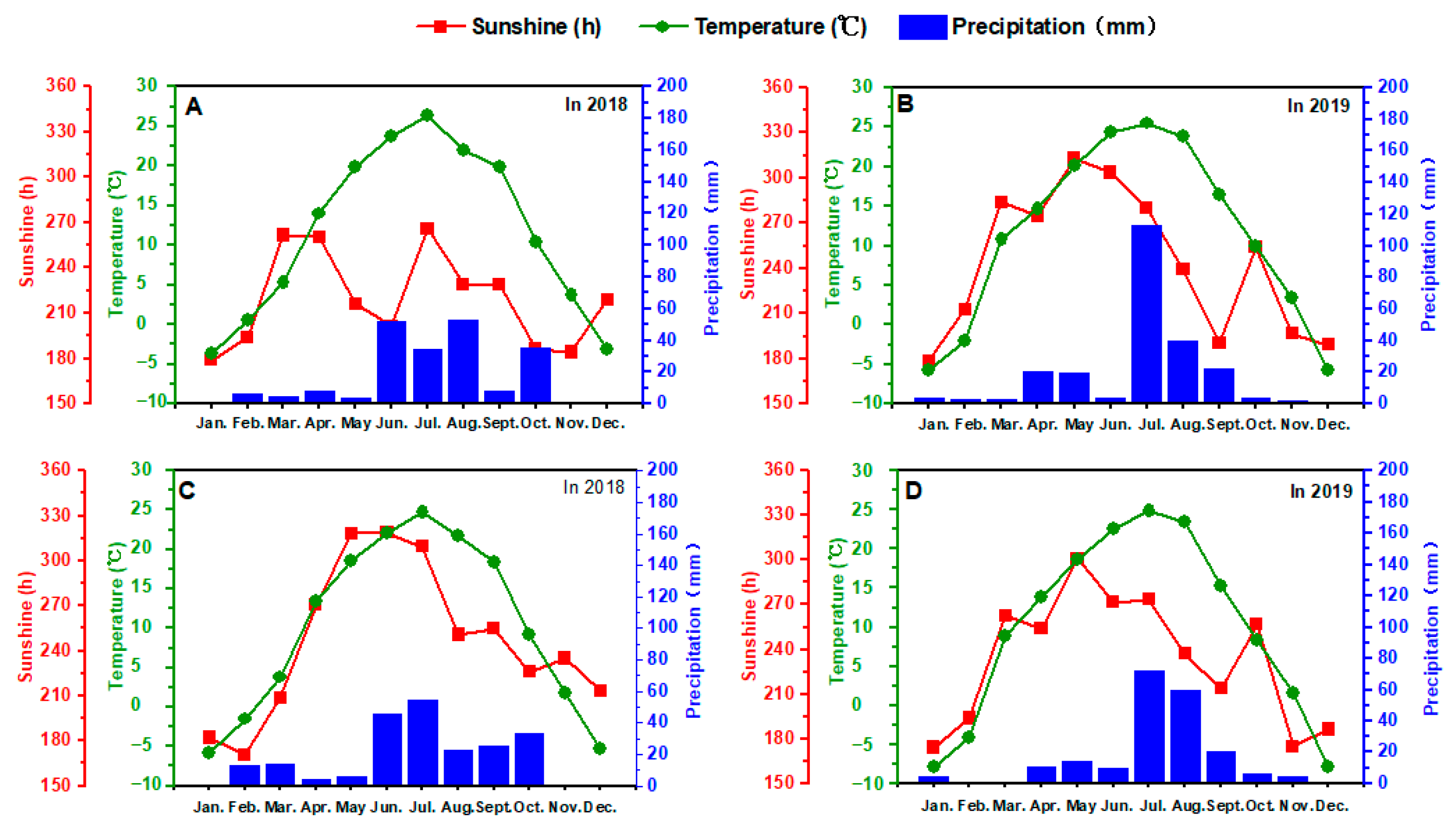
Figure 1. Temporal distribution of monthly average temperature, precipitation, and sunshine hours. (A,B) represent the meteorological data of the Zhongning County study area in 2018 and 2019, respectively. (C,D) represent the meteorological data of the Nuanquan Farm study area in 2018 and 2019, respectively.
Agronomy 15 02072 g001
Figure 2. Reflectance curves of OS, FDS, and CRS of the wolfberry canopy from 400 nm to 1300 nm. OS presents the original spectra; FDS presents the first-derivative spectra; CRS presents the continuum-removal spectra (maximum value = 1). Each coloured line represents a sample reflectance curve, with a total of 95 samples in total.
Agronomy 15 02072 g002
Figure 3. Distribution of correlation coefficients between canopy spectral reflectance and nitrogen content. (A–C) represent the correlation coefficients of the original spectra (OS), continuum-removed spectra (CRS), and first-derivative spectra (FDS) with nitrogen content, respectively.
Agronomy 15 02072 g003
Figure 4. Heat maps of correlation coefficients between the ratio spectral index (RSI) and nitrogen content. (AC) represent the original spectra (OS), continuum-removed spectra (CRS), and first-derivative spectra (FDS), respectively.
Agronomy 15 02072 g004
Figure 5. Feature significance of the spectral variables significantly correlated with nitrogen content at the 0.01 level. (AC) represent the original spectra (OS), continuum-removed spectra (CRS), and first-derivative spectra (FDS), respectively.
Agronomy 15 02072 g005
Figure 6. Feature significance of the spectral variables significantly correlated with nitrogen content at the 0.01 level. (AD) correspond to the published vegetation indices (PVIs), the ratio spectral indices derived from the original spectra (RSI-OS), the ratio spectral indices derived from the continuum-removed spectra (RSI-CRS), and the ratio spectral indices derived from the first-derivative spectra (RSI-FDS), respectively.
Agronomy 15 02072 g006
Figure 7. Performance metrics of the multivariate regression models based onthe training dataset. (AC) correspond to the coefficient of determination (R2), root mean square error (RMSE), and mean absolute error (MAE) for models using original, continuum-removal, and first-derivative spectra, respectively. (DF) represent R2, RMSE, and MAE for models using ratio spectral indices derived from original spectra (RSI-OS), continuum-removal spectra (RSI-CRS), and first-derivative spectra (RSI-FDS), respectively.
Agronomy 15 02072 g007
Figure 8. Distribution of measured and predicted values of the nonlinear multivariate regression models for the test dataset using different spectral preprocessing techniques. (a) Models developed from original spectra (OS): (A-1) (RF), (B-1) (Adaboost), (C-1) (Extra Trees), (D-1) (CatBoost), and (E-1) (XGBoost). (b) Models developed from continuum-removal spectra (CRS): (A-2) (RF), (B-2) (Adaboost), (C-2) (Extra Trees), (D-2) (CatBoost), and (E-2) (XGBoost). (c) Models developed from first-derivative spectra (FDS): (A-3) (RF), (B-3) (Adaboost), (C-3) (Extra Trees), (D-3) (CatBoost), and (E-3) (XGBoost).
Agronomy 15 02072 g008
Figure 9. Distribution of measured and predicted values for nonlinear multivariate regression models for the test dataset based on different spectral indices. (a) Models based on published vegetation indices (PVIs): (A-0) (RF), (B-0) (Adaboost), (C-0) (Extra Trees), (D-0) (CatBoost), and (E-0) (XGBoost). (b) Models based on ratio spectral indices derived from original spectra (RSI-OS): (A-1) (RF), (B-1) (Adaboost), (C-1) (Extra Trees), (D-1) (CatBoost), and (E-1) (XGBoost). (c) Models based on ratio spectral indices derived from continuum-removal spectra (RSI-CRS): (A-2) (RF), (B-2) (Adaboost), (C-2) (Extra Trees), (D-2) (CatBoost), and (E-2) (XGBoost). (d) Models based on ratio spectral indices derived from first-derivative spectra (FDS): (A-3) (RF), (B-3) (Adaboost), (C-3) (Extra Trees), (D-3) (CatBoost), and (E-3) (XGBoost).
Agronomy 15 02072 g009
Figure 10. RPD distribution of the multivariate nonlinear regression methods. The red dashed line indicates the threshold of RPD = 1.4, distinguishing poor predictive performance (RPD < 1.4) from good estimation capability (1.4 ≤ RPD < 1.8), as defined by the RPD evaluation criteria in Section 2.4.
Agronomy 15 02072 g010
Table 1. Phenological characteristics of the wolfberry tree [31].
DatePhenological Characteristics
Early AprilThe wolfberry tree begins to sprout and develop new leaves.
Late April to early MayNew branches exhibit vigorous growth, with the emergence of buds and a few flowers.
Late May to early AugustThe period marks the flowering and fruiting phase for summer fruits.
Mid-August to SeptemberAs old leaves begin to fade, new buds open, and fresh branches extend, the plant enters the autumn flowering and fruiting stage.
October to NovemberPlants shed leaves and transition into dormancy.
Table 2. Summary of published vegetation indices used for nitrogen content estimation. Rλ and Dλ refer to the original spectral reflectance and the first-derivative spectral reflectance at wavelength λ nm, respectively.
Vegetation IndicesCalculation FormulaReference
RVIR800/R670[35]
GMR750/R700[36]
SR705R750/R705[37]
SR550,670R550/R670[38]
Ratio vegetation index (VOG1)R740/R720[39]
Ratio vegetation index (GM1)R750/R550[40]
Ratio vegetation index (RVI1)R950/R660[41]
RVI (R780,R550)R780/R550[38]
RVI (R780,R670)R780/R670[38]
GI (Greenness index)R554/R677[42]
RVI (D705,D722)D705/D722[43]
RVI (D730,D706)D730/D706[43]
Canopy chlorophyll index (CCI)D720/D700[44]
Datt derivative (DD)D755/R705[45]
ND705(R750 − R705)/(R750 + R705)[37]
NDVIgb(R573 − R440)/(R573 + R440)[46]
PPR(R550 − R450)/(R550 + R450)[47]
PRI(R570 − R531)/(R570 + R531)[48]
GNDVI(R750 − R550)/(R750 + R550)[49]
NPCI(R430 − R680)/(R430 + R680)[50]
NRI(R570 − R670)/(R570 + R670)[51]
SIPI(R810 − R460)/(R810 + R460)[52]
NDVI(R800 − R670)/(R800 + R670)[53]
Normalized difference vegetation index(NDVI1)(R790 − R670)/(R790 + R670)[54]
Normalized difference vegetation index (NDVI2)(R1220 − R710)/(R1220 + R710)[41]
Revised normalized difference vegetation index (ReNDVI)(R755 − R705)/(R755 + R705)[55]
Normalized difference red edge index (NDRE)(R790 − R720)/(R790 + R720)[56]
NDI(R780 − R670)/(R780 + R670)[38]
Table 3. Descriptive Statistics of Nitrogen Content in Samples.
Sample SizenMaximumMinimumMeanStandard DeviationCoefficient of Variation
Total set954.6602.9004.0840.3749.158%
Training set634.6602.9004.0770.3819.345%
Test set324.6303.1104.0980.3658.907%
Table 4. Correlation coefficients of published vegetation indices with nitrogen content. *** and ** represent significant correlation at the p < 0.01 and p < 0.05 levels, respectively.
Vegetation IndexCorrelation CoefficientVegetation IndexCorrelation Coefficient
RVI0.321 ***ND7050.319 ***
GM0.322 ***NDVIgb0.366 ***
SR7050.319 ***PPR0.356 ***
SR(550 670)0.335 ***PRI−0.367 ***
VOG10.284 ***GNDVI0.297 ***
GM10.297 ***NPCI0.205 **
RVI10.323 ***NRI0.336 ***
RVI (R780 R550)0.300 ***SIPI0.314 ***
RVI (R780 R670)0.323 ***NDVI0.321 ***
GI (Greenness index)0.333 ***NDVI10.321 ***
RVI (D705 D722)−0.041NDVI20.282 ***
RVI (D730 D706)0.158ReNDVI0.319 ***
CCI0.223 **NDRE0.270 ***
DD0.202**NDI0.323 ***
Table 5. The main parameters of the models.
ModelModel Parameters
RFn_estimators = 100, max_depth = 10, min_samples_split = 2, min_samples_leaf = 1
AdaBoostn_estimators = 100, learning_rate = 1, Loss function = square, base_estimator = Decision Tree Classifier
ExtraTreesn_estimators = 100, max_depth = 10, min_samples_split = 2, min_samples_leaf = 1
CatBoostIterations = 100, learning_rate = 0.06, depth = 10, l2_leaf_reg = 5
XGBoostmax_depth = 10, learning_rate = 0.06, n_estimators = 100, l2_leaf_reg = 5
GDLRlearning_rate = 0.05, max_iter = 100, batch_size = BGD, penalty = ‘l2’, alpha = 0.05, fit_intercept = True, tol = 1 × 10⁻⁴,
OLSLRfit_intercept = True, normalize = False, copy_X = True, positive = False,
RRalpha = 0.5, fit_intercept = True, max_iter = 300, solver = ‘cholesky’, tol = 1 × 10⁻⁴
Disclaimer/Publisher’s Note: The statements, opinions and data contained in all publications are solely those of the individual author(s) and contributor(s) and not of MDPI and/or the editor(s). MDPI and/or the editor(s) disclaim responsibility for any injury to people or property resulting from any ideas, methods, instructions or products referred to in the content.