Spectral Estimation of Nitrogen Content in Cotton Leaves Under Coupled Nitrogen and Phosphorus Conditions

Abstract

With the increasing application of hyperspectral technology, rapid and accurate monitoring of cotton leaf nitrogen concentrations (LNCs) has become an effective tool for large-scale areas. This study used Tahe No. 2 cotton seeds with four nitrogen levels (0, 200, 350, 500 kg ha⁻¹) and four phosphorus levels (0, 100, 200, 300 kg ha⁻¹). Spectral data were acquired using an ASD FieldSpec HandHeld2 portable spectrometer, which measures spectral reflectance covering a band of 325–1075 nm with a spectral resolution of 1 nm. LNCs determination and spectral estimation were conducted at six growth stages: squaring, initial bloom, peak bloom, initial boll, peak boll, and boll opening. Thirty-seven spectral indices (SIs) were selected. First derivative (FD), standard normal variate (SNV), multiplicative scatter correction (MSC), and Savitzky–Golay (SG) were applied to preprocess the spectra. Feature bands were screened using partial least squares discriminant analysis (PLS–DA), and support vector machine (SVM) and random forest (RF) models were used for accuracy validation. The results revealed that (1) LNCs initially increased and then decreased with growth, peaking at the full-flowering stage before gradually declining. (2) The best LNC recognition models were SVM–MSC in the squaring stage, SVM–FD in the initial bloom stage, SVM–FD in the peak bloom stage, SVM–FD in the initial boll stage, RF–SNV in the peak boll Mstage, and SVM–FD in the boll opening stage. FD showed the best performance compared with the other three treatments, with SVM outperforming RF in terms of higher R² and lower RMSE values. The SVM–FD model effectively improved the accuracy and robustness of LNCs prediction using hyperspectral leaf spectra, providing valuable guidance for large-scale information production in high-standard cotton fields.

1. Introduction

Cotton (Gossypium hirsutum) is a highly valuable cash crop [1]. In Xinjiang, with suitable lighting conditions, advanced planting management technology, and large-scale high-standard farmland, Xinjiang has become the largest high-quality cotton production area in China. It is particularly important to apply fertilizer reasonably, further prevent soil salinization, and maintain the sustainable development of efficient farmland. However, the blind increase in the current application of chemical fertilizers not only leads to a rise in production costs but also triggers a series of environmental problems. Therefore, precisely monitoring the nutrient requirements during the growth process of cotton is particularly crucial for achieving precise fertilization and sustainable agricultural development.

Nitrogen is an elemental nutrient that has a decisive effect on crop yield, growth, and quality. Its key role in cotton development has been widely recognized [2]. Nitrogen content significantly affects the chlorophyll concentration in leaves, thereby altering the light absorption and reflection in the visible and near-infrared regions. Phosphorus is a sensitive element of cotton [3]. Fluctuations in phosphorus levels can obviously affect the growth, development, and yield of cotton. Continuous excessive application of phosphate fertilizer can increase the soil phosphorus content, thereby increasing production costs, causing environmental pollution [4], and restricting the sustainable development of cotton production. Phosphorus deficiency can lead to structural and physiological changes in leaves, thereby affecting leaf reflectance. An appropriate level of phosphorus can enhance the efficiency of nitrogen fertilizer utilization, thereby altering the spectral performance of nitrogen in plant tissues. The traditional methods for monitoring the nitrogen concentration in crop leaves mainly rely on destructive determination means such as chemical analysis, for example, the Kjeldahl nitrogen determination method. These methods are not only cumbersome to operate, time-consuming, and labor-intensive, but also, due to the need for sampling and sample processing, it is difficult to achieve large-scale rapid monitoring. The monitoring range is limited and cannot meet the demands of modern agricultural production for real-time and large-scale nutrient monitoring [5,6]. With the continuous development of remote sensing technology, hyperspectral remote sensing technology has the advantages of hyperspectral resolution, wide coverage, convenient data acquisition, etc., and has shown crucial potential in monitoring crop leaf nitrogen concentrations (LNCs) changes [7]. With the continuous popularization and promotion of hyperspectral remote sensing technology, it has become an effective means to rapidly diagnose LNCs and other indicators of crop leaves [8,9,10,11]. By analyzing the relationship between spectral characteristics and nitrogen content, it can achieve non-destructive and rapid diagnosis of the nitrogen nutritional status of crops, which is of great significance for guiding precise fertilization.

In addition, in previous studies on the spectral estimation of the crop LNCs, a spectral index (SI) was constructed by the sum, difference, and ratio of the spectral reflectances of two or more bands that are highly correlated with the crop LNCs [12,13,14]. Wang et al. [15] constructed a new multiangle blue edge absorption vegetation index (MBEAVI) by collecting spectral data of cotton leaves at different growth stages and at different leaf inclination angles through hyperspectral imaging technology combined with the cotton leaf nitrogen concentrations (LNCs) measured in the laboratory. The MBEAVI model, which is based on multiangle spectral data, had greater accuracy and stability in predicting cotton LNCs than the single-angle model. The R² value of the MBEAVI model reached 0.812, which was significantly greater than the value of 0.735 of the optimized red-edge absorption (OREA) model. The R² value of the MBEAVI model in the interannual test was 0.789. Many studies have shown that for the monitoring of crop LNCs, the extraction of sensitive bands by means of pretreatment [16,17], SI [18,19], and screening algorithms [20,21] can enhance the correlation of the original spectra and thus improve the precision of crop nitrogen content determination via a series of inversion models. This provides an effective means for crop LNC monitoring. Many mature studies have monitored crop LNCs by hyperspectral remote sensing technology. Moreover, machine learning algorithms have been widely used in the construction of hyperspectral monitoring models, and monitoring crop growth has attracted the attention of scholars [22,23,24,25]. Moreover, machine learning algorithms have been continuously applied in modern agriculture, injecting great impetus into the development of agricultural informatization. Most studies have focused on the extraction of cotton canopy feature information, monitoring of diseases and pests in cotton fields, and evaluating cotton growth [21,26,27]. However, there have been few reports on the different growth stages and the coupling modes of nitrogen and phosphorus in cotton fields by hyperspectral techniques. Therefore, the spectral characteristics of cotton leaves and the coupling of nitrogen and phosphorus in different growth stages can potentially be studied via hyperspectral technology.

In summary, this study investigated the variation in LNCs and leaf spectral curves of cotton at different growth stages under different nitrogen and phosphorus application amounts. By integrating SI and partial least square discriminant analysis (PLS–DA) to extract the variable importance projection (VIP) values between 325 and 1075 nm and identify the optimal band, a support vector machine (SVM) and random forest (RF) were used to establish the optimal cotton LNCs model. This study provides a theoretical basis for realizing large-area remote sensing monitoring of nitrogen and phosphorus applications in cotton. The main aims of this study are as follows: (1) clarify the variation in cotton LNCs under different nitrogen and phosphorus coupling conditions at different growth stages and provide a scientific basis for nutrient management of cotton in precision agriculture; (2) establish a diagnostic model of cotton nitrogen and phosphorus nutrition under different pretreatments at different growth stages on the basis of the combination of spectral characteristics and PLS–DA and formulate an optimal model under different pretreatments at different growth stages to realize rapid and nondestructive monitoring of cotton growth and nutrient requirements.

2. Materials and Methods

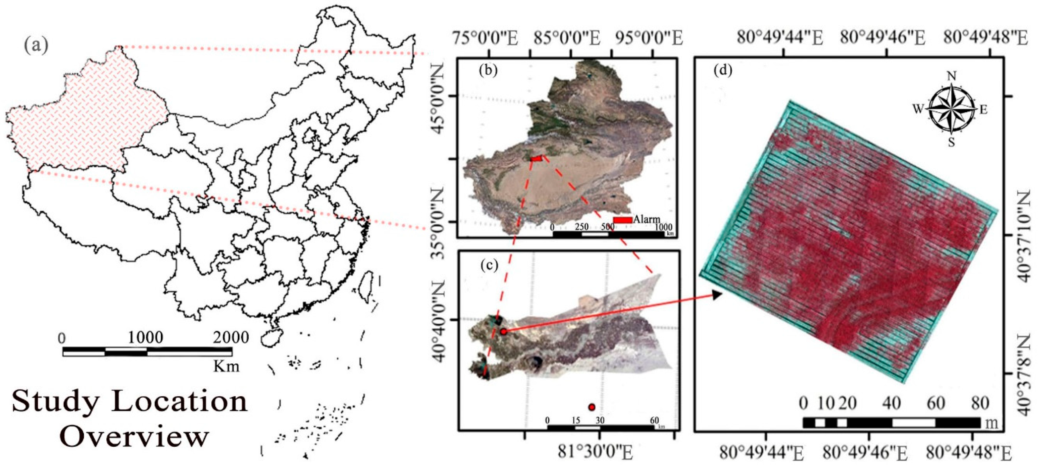
2.1. Overview of the Study Area

The research area was located at the Aksu National Field Scientific Observation and Research Station for Farmland Ecosystem, Chinese Academy of Sciences, Xinjiang, with geographical coordinates of 80°49′ W, 40°37′ N and an altitude of 1028 m. The station was located in the plain desert-oasis area near the junction point of the three sources of the Tarim River. The climate is warm temperate arid, the temperature is high in summer and low in winter, and the temperature changes sharply in spring and autumn. The annual average precipitation is 45.7 mm, which means that the area mainly relies on alpine precipitation and ice and snow melting to supply water. The annual average temperature is 11.2 °C, the frost-free period is 207 days, the annual sunshine duration is 2940 h, and the annual average wind speed is 2.4 m/s. After the application of cotton field base fertilizer, fertilization was carried out in late June and early August 2024. Urea was used for nitrogen fertilizer, potassium dihydrogen phosphate was used for phosphate fertilizer, and potassium sulfate was used for potassium fertilizer. The application was divided into 6 steps at each of the 6 growth stages. The research area is shown in Figure 1.

2.2. Experimental Design

The Batuan National Field Scientific Observation and Research Station in Aksu District of Xinjiang was selected as the test site for the salinized cotton field. The selected cotton variety was Tahe II. Different levels of nitrogen and phosphorus were set for different gradients, and four water types were set for nitrogen application: 0 (N₀) kg ha⁻¹, 200 (N₁) kg ha⁻¹, 350 (N₂) kg ha⁻¹, and 500 (N₃) kg ha⁻¹. Four levels of phosphorus application were set, namely, 0 (P₀) kg ha⁻¹, 100 (P₁) kg ha⁻¹, 200 (P₂) kg ha⁻¹, and 300 (P₃) kg ha⁻¹, and potassium sulfate 169 kg ha⁻¹, in a total of 16 plots, and each plot was repeated 6 times. Each plot had three membranes, and three rows of cotton were planted on each membrane. The experiment selected 6 cotton stages for determination, namely, the squaring stage, initial bloom stage, peak bloom stage, initial boll stage, peak boll stage, and boll opening stage. Cotton samples and data were collected under the above different nitrogen and phosphorus application gradients. A total of 96 samples were collected during each growth period, from which 2/3 of the samples were randomly selected as the training set and the remaining samples were used as the verification set. The SVM and RF were used to establish the cotton LNCs prediction model, and the accuracy of the model was tested by analysis and comparison.

2.3. Data Acquisition

2.3.1. Collection and Determination of Cotton Samples

Cotton samples were sown in early April and collected from June to August 2024. The total area of cotton fields in the test area was 0.33 ha. The cotton variety used was Tahe No. 2, and the planting mode included three rows of film in each plot, with six rows of cotton planted on each film. The samples were collected at the squaring stage, initial bloom stage, peak bloom stage, initial boll stage, peak boll stage and boll opening stage, and the collected cotton plants were packed into an incubator, brought back to the laboratory, and placed in a constant-temperature drying oven. After the temperature in the box was raised to 105 °C, the cotton plants were allowed to grow for half an hour and then dried to a constant weight at 85 °C. After the dry matter was weighed, the samples were ground and boiled with H₂SO₄-H₂O₂. The LNCs was determined by a Kjeldahl nitrogen analyzer, and its calculation formula is as follows:

$$\omega \left(N\right)=(c\left(V-V_0\right)\times 0.014\times D\times 100)/\mathrm{m}$$

(1)

where $\omega \left(N\right)$ is the total nitrogen content of the leaf sample, in %; c is the concentration of an acid standard solution (usually sulfuric acid), in mol/L; V is the volume of acid standard solution used in the titration, in mL; V₀ is the volume of acid standard solution used when titrating the blank, in mL; 0.014 is the molar mass of nitrogen, in kg/mol; D is the ratio of the constant volume (V₁) (mL) of the boiling liquid to the volume (V₂) (mL) of the absorption measurement, that is, the dilution multiple; 100 is used to convert the value to %; and m is the mass of the sample, in g.

2.3.2. Determination of the Spectral Data of the Cotton Leaf

The cotton samples were collected in clear and windless weather. In this study, an ASD FieldSpecHandHeld2 portable ground object spectrometer was used to obtain the spectral information of the sampled cotton leaves. The instrument was used to measure spectral reflectance covering a band of 325–1075 nm, and the spectral resolution was 1 nm. The reflectance obtained was derived from the cotton leaf, which had no pests or diseases, no lack of seedlings or ridges, and a uniform growth state. After the spectral values of 5 cotton leaves at each point were measured, the average value was taken as the average reflectance of the point.

2.4. Data Processing and Analysis

2.4.1. Screening Feature Band

Most studies have shown that data fusion can reduce data limitations and thus increase target accuracy [28,29]. After smoothing the original waveband through Savitzky–Golay (SG) [30] convolution and then pretreatment with first derivation (FD), standard normal variate (SNV), multiplicative scatter correction (MSC) and SG, four pretreated leaves spectral reflectances were obtained. Furthermore, the first 20 bands with VIP values > 1 between 325 and 1075 nm were extracted via PLS–DA at different growth stages, and the LNCs of cotton and the SI with a p-value < 0.01 were fused. The characteristic variables extracted by these two methods were combined as input vectors for modeling.

The VIP value in PLS–DA was used to evaluate the degree of contribution of different independent variables to the dependent variables in multivariate statistical analysis to help select the optimal set of independent variables and to reflect the importance of each independent variable by calculating its degree of contribution to the PLS model [31]. PLS-DA can not only effectively extract the feature variables highly correlated with the target variable but also retain the main features and information of the data while reducing the dimension. The larger the VIP value is, the greater the contribution of the independent variable to the dependent variable. Therefore, the independent variable with a higher VIP value can be preferentially selected for establishing the model. In practice, variables with VIP values greater than 1 are usually reserved. In this study, the top 20 variables with high VIP values were extracted as characteristic variables.

The SI is an index calculated on the basis of remote sensing data by combining and comparing spectral features, such as the reflectance and emissivity in different wavelength ranges [32]. They can be used to characterize land cover type, growth state, vegetation content, soil properties and other information and are often used in the research and monitoring of agriculture, the ecological environment, water resources and other fields. This study selected 37 SIs, as shown in

Table 1. SI formulas.

Spectral Index	Formula	Document Source
DVI	R 800−R 680	Richardson et al. [33]
mND705	(R750 − R705)/(R750 + R705 − 2 × R445)	Sims et al. [34]
mSR705	(R750 − R445)/(R705 − R445)	Sims et al. [34]
PRI	(R570 − R531)/(R570 + R531)	Gamon et al. [35]
MTCI	(R750 − R710)/(R710 − R680)	Dash et al. [36]
MCARI	[(R700 − R670) − 0.2 × (R700 − R550)] × (R700/R 670)	Dash et al. [36]
OSAVI	(1 + 0.16) × (R800 − R670)/(R800 + R670 + 0.16)	Rondeaux et al. [37]
TCARI	3 × [(R700 − R670) − 0.2 × (R700 − R550)] × (R700/R670)	Haboudane et al. [38]
NDVI705	(R750 − R705)/(R750 + R705)	Gitelson et al. [39]
NDVI550	(R750 − R550)/(R750 + R550)	Gamon et al. [35]
VOG1	R740/R720	Zarco-Tejada et al. [40]
VOG2	(R734 − R 747)/(R715 + R 726)	Zarco-Tejada et al. [40]
VOG3	(R734 − R747)/(R715 + R 720)	Zarco-Tejada et al. [40]
VOG4	R780/R740	Wang et al. [41]
SR1	R985/R745	Schlerf et al. [42]
SR2	R675/R700	Liang et al. [43]
VARI	(R555 − R680)/(R580 + R680 + R480)	Wang et al. [41]
CIred edge	R750/R705 − 1	Hong et al. [44]
RI-half	R747/R708	Hong et al. [44]
Carte1	R695/R420	Liang et al. [43]
Carte2	R695/R760	Liang et al. [43]
Carte3	R710/R760	Liang et al. [43]
Datt1	(R850 − R710)/(R850 + R680)	Liang et al. [43]
Datt2	R850/R710	Liang et al. [43]
Datt3	R754/R704	Liang et al. [43]
NVI	(R777 − R747)/R673	Liang et al. [43]
NRI	(R570 − R670)/(R570 + R670)	Fu et al. [45]
Lichtenthaler	R440/R690	Sun et al. [46]
ND	(R935 − R705)/(R935 + R705)	Sun et al. [46]
CIgreen	R800/R550 − 1	Sun et al. [46]
GARI	[R800 − [R550 − 1.7 × (R470 − R670)]]/ [R800 + [R550 − 1.7 × (R470 + R670)]]	Chen et al. [47]
REP	700 + 40 × [(R670 + R780)/2-R700]/(R740 − R700)	Liang et al. [43]
SPVI	0.4 × 3.7 × (R670 − R550) − 1.2 × |R530 − R670|	Liang et al. [43]
SPVI2	0.4 × 3.7 × (R800 − R670) − 1.2 × |R550 − R670|	Liang et al. [43]
RVSI	(R714 + R752)/2 − R733	Naidu et al. [48]
HI	(R534 − R698)/(R534 + R698) − 0.5R704	Mahlein et al. [49]
NSRI	R890/R780	Liu et al. [50]

.

2.4.2. Model Construction and Accuracy Checking

The data processing software R 4.3.2 was used for data analysis and graph drawing. MATLAB R2022a was used to preprocess the original spectral data, run the SVM and RF models, and then establish the optimal cotton LNCs model.

SVM is a powerful classification algorithm that differentiates different classes of data by finding an optimal hyperplane in the feature space. This hyperplane maximizes the spacing between the two classes to improve the generalization ability of the model. SVMs can also handle nonlinear problems and map data to high-dimensional spaces through kernel techniques to achieve more complex boundary partitioning [51].

RF is an ensemble learning algorithm that improves the accuracy and stability of a model by building multiple decision trees and combining their predictions. It constructs each tree by randomly selecting samples and features, reduces overfitting, and is suitable for classification and regression problems [52].

The model accuracy evaluation mainly includes the determination coefficient (R²), root mean square error (RMSE), and Lin’s concordance correlation coefficient (LCCC) [53]. LCCC is a statistical indicator used to assess the consistency between the predicted results of the model and the true value. It not only measures the linear relationship between the predicted and the true value but also takes into account the bias and scale changes, which can more comprehensively assess the accuracy and accuracy of the model. The larger the R² is, the smaller the RMSE is, and the higher the LCCC is, the better the prediction effect. The formulas are as follows:

$${\mathrm{R}}^2=1-{\displaystyle \frac{\sum _{i=0}^n{{(LNC}_i-{LNCP}_i)}^2}{{\sum }_{i=0}^n{({LNC}_i-\overline{{LNC}_i})}^2}}$$

(2)

$$\mathrm{RMSE}=\sqrt{{\displaystyle \frac{{\sum }_{i=0}^n{{(LNC}_i-{LNCP}_i)}^2}{n}}}$$

(3)

$$\mathrm{LCCC}={\displaystyle \frac{2r{S_{LNC}S}_{LNCP}}{{S^2}_{LNC}+{S^2}_{LNCP}+{(\overline{{LNC}_i}-\overline{{LNCP}_i)}}^2}}$$

(4)

where LNCs is the measured value of the total nitrogen content in cotton leaves; LNCP is the predicted value of the model for estimating the total nitrogen content in cotton leaves; $\overline{{LNC}_i}$ and $\overline{{LNCP}_i}$ are the average values of the measured and predicted total nitrogen contents in the cotton leaves, respectively; n represents the number of cotton leaf samples; r represents the correlation coefficient between the measured and predicted total nitrogen contents in the cotton leaves; and $S_{LNC}$ and $S_{LNCP}$ are the variances of the measured and predicted values, respectively.

3. Results

3.1. Cotton LNCs Variations at Different Growth Stages Under Different Nitrogen and Phosphorus Coupling Conditions

The cotton LNC variations under different nitrogen and phosphorus coupling conditions represent the changes in the LNCs of all the sampled cotton plants under different nitrogen and phosphorus coupling conditions.

As shown in Figure 2, the overall LNC content of cotton tended to first increase but then decrease through the different growth stages, among which the LNCs were highest at the full flowering stage and then tended to decrease. Under varying nitrogen and phosphorus conditions, the LNC content was highest at the N₃P₁ treatment during the squaring stage (1.16%), at the N₃P₀ treatment during the initial bloom stage (1.30%), at the N₂P₂ treatment during the peak bloom stage (1.60%), at the N₂P₂ treatment during the initial boll stage (1.24%), at the N₀P₃ treatment during the peak boll stage (1.16%), and at the N₃P₂ treatment during the boll opening stage (1.12%).

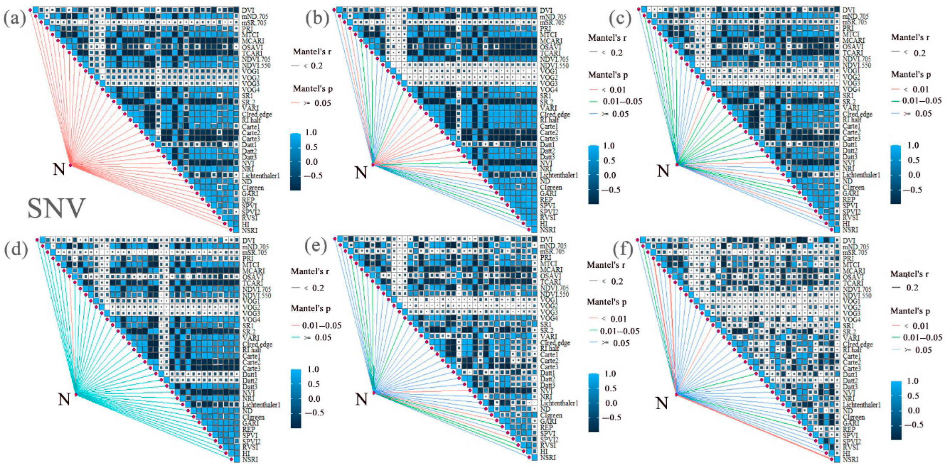
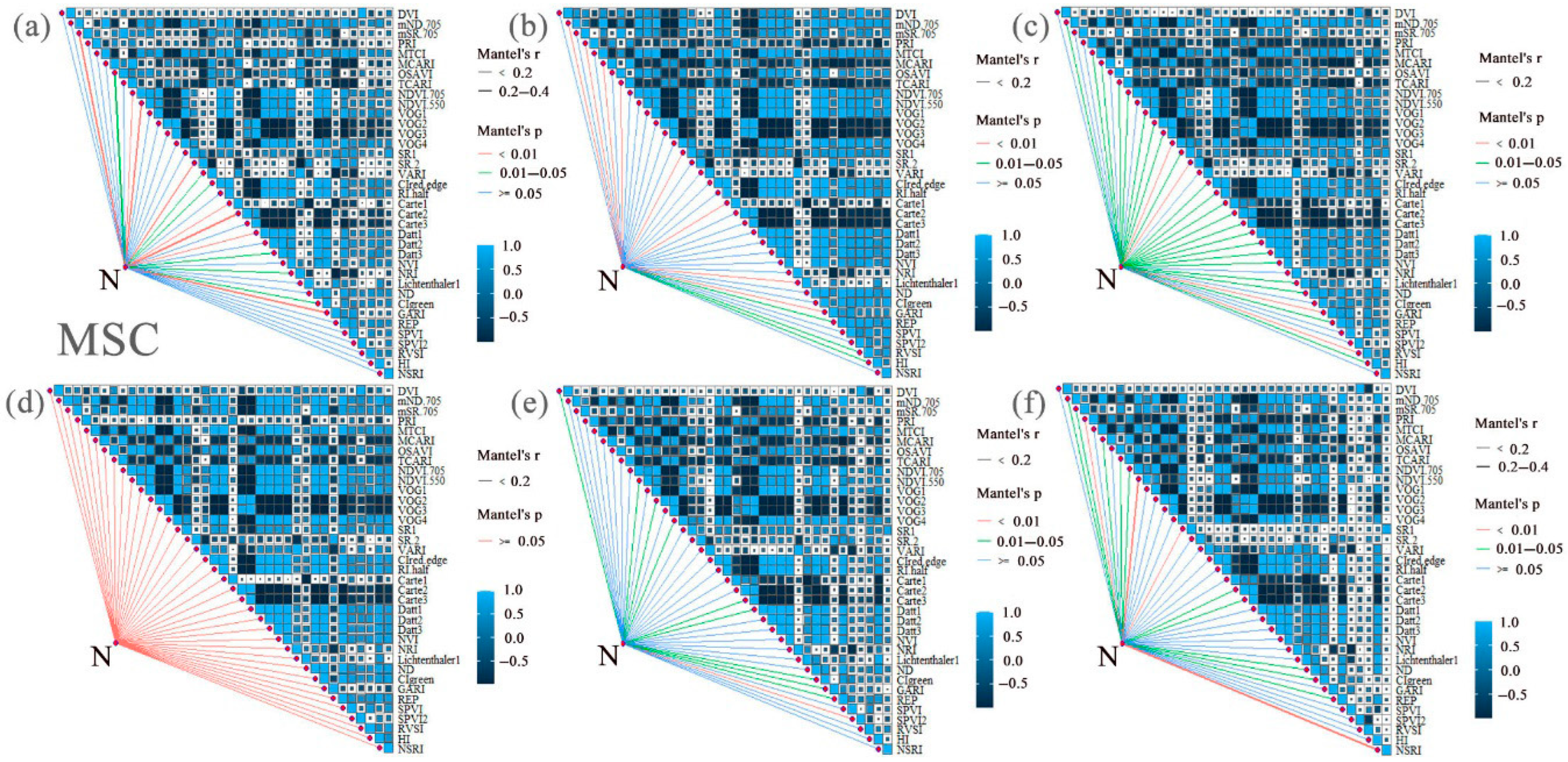
3.2. Correlation Analysis and Extraction of LNCs and SIs from Cotton Under Different Nitrogen and Phosphorus Coupling Conditions

All the original spectra were smoothed via Savitzky–Golay smoothing with MATLAB, and then FD, SNV and MSC preprocessing treatments were adopted. R 4.3.2 software was used to conduct Mantel test heatmap analysis and map the LNCs and SIs of cotton at different growth stages. The heatmap analysis after FD preprocessing is shown in Figure 3.

As shown in Figure 3, after FD pretreatment, the initial bloom stage showed the highest correlation, with seven SIs having a p-value < 0.01, with SRI exhibiting the highest R value (0.51). As shown in Figure 4, after SNV pretreatment, the initial bloom stage also demonstrated the highest correlation, with 13 SIs having a p-value < 0.01, particularly SR2 (R value 0.51). As shown in Figure 5 and Figure 6, following MSC and SG pretreatments, the initial bloom stage generally performed better than other stages, but the differences in peak bloom, peak boll, and boll opening stages were not significant.

In summary, the SIs with a p-value < 0.01 in the different growth stages under FD, SNV, MSC, and SG pretreatment were selected as the integration vectors for subsequent modeling, as shown in

Table 2. SIs extracted at different growth stages under different pretreatment conditions.

SP	Stage	Spectral Index
FD	Squaring	/
	Initial bloom	mND705, PRI, MCARI, TCARI, SRI, Lichtenthaler1, GARI
	Peak bloom	VOG4, SR2, GARI, RVSI
	Initial boll	/
	Peak boll	SPVI2
	Boll opening	PRI, NDVI550, SR1, NSRI
SNV	Squaring	/
	Initial bloom	mND705, PRI, SP1, SR2, Clred edge, RI-half, Carte1, Carte2, Carte3, Datt2, Datt3, Lichtenthaler1, ND
	Peak bloom	VOG4, NVI, ND, RVSI
	Initial boll	SPVI2
	Peak boll	NVI, GARI, SPVI
	Boll opening	PRI, OSAVI, SR1, NSRI
MSC	Squaring	mSR705, NDVI705, NDVI550, SR2, Clarte1, Carte2, Datt1, GARI
	Initial bloom	mND705, PRI, MCARI, TCARI, SR1, Carte1, Lichtenthaler1, GARI
	Peak bloom	VOG4, SR2, GARI, RVSI
	Initial boll	/
	Peak boll	SPVI2
	Boll opening	PRI, NDVI550, SR1, NSRI
SG	Squaring	NDVI705, NDVI550, SR2, Clarte1, Carte2, Datt1, GARI
	Initial bloom	mND705, PRI, MCARI, TCARI, SR1, Carte1, Lichtenthaler1, GARI
	Peak bloom	VOG4, SR2, GARI, RVSI
	Initial boll	/
	Peak boll	SPVI2
	Boll opening	PRI, NDVI550, SR1, NSRI

Note: “/” indicates no SI at the p-value < 0.01.

:

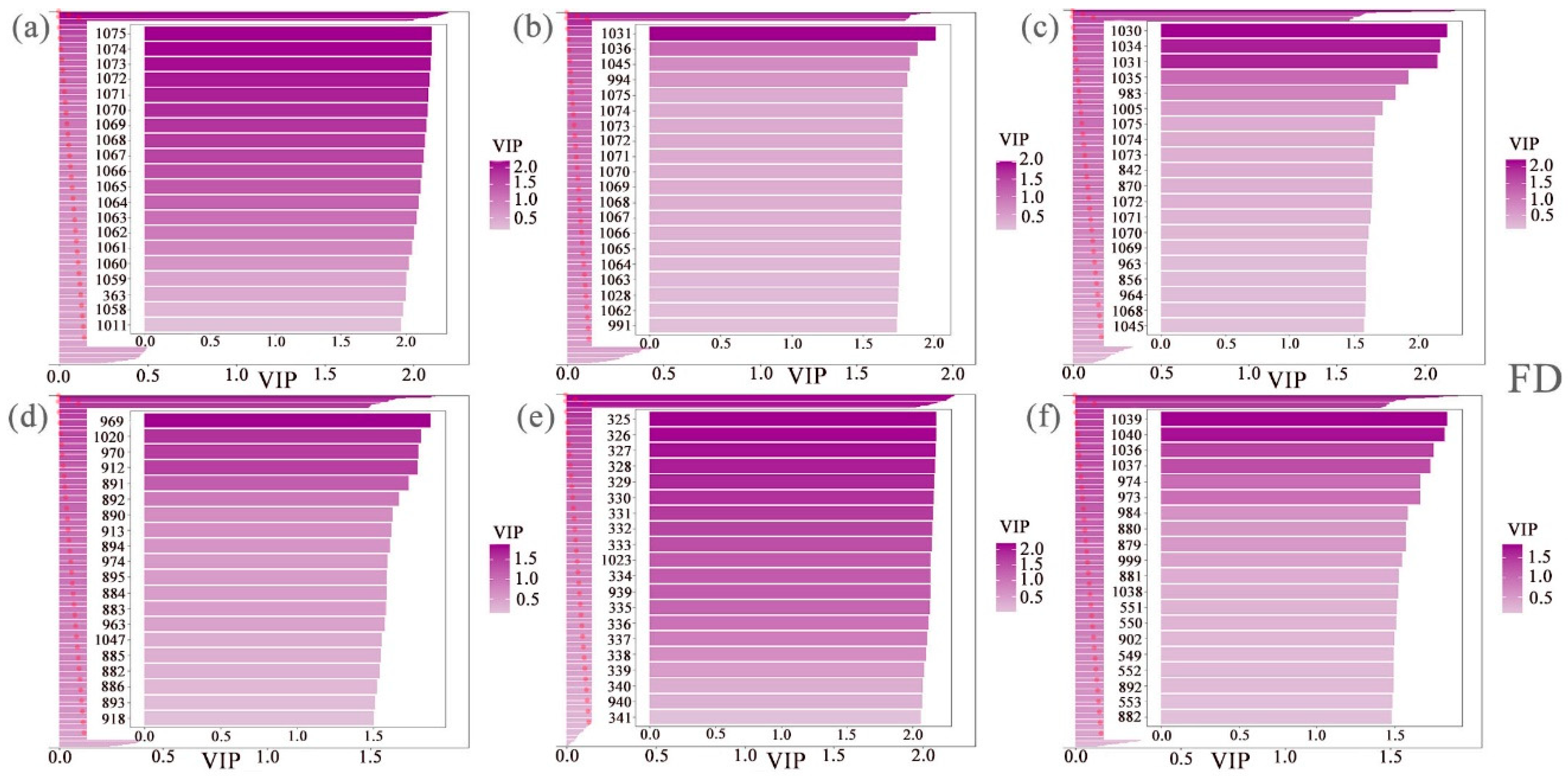
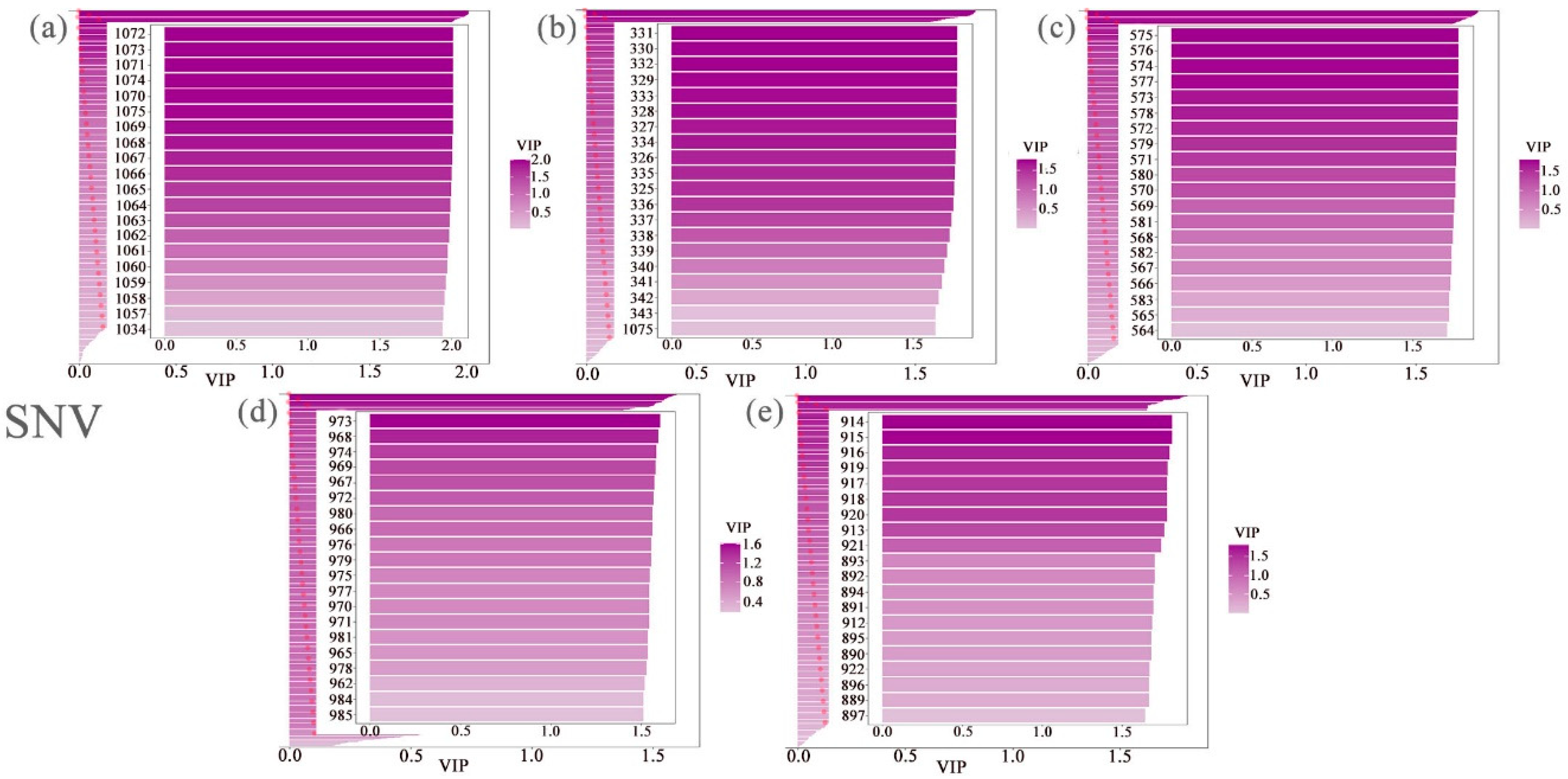
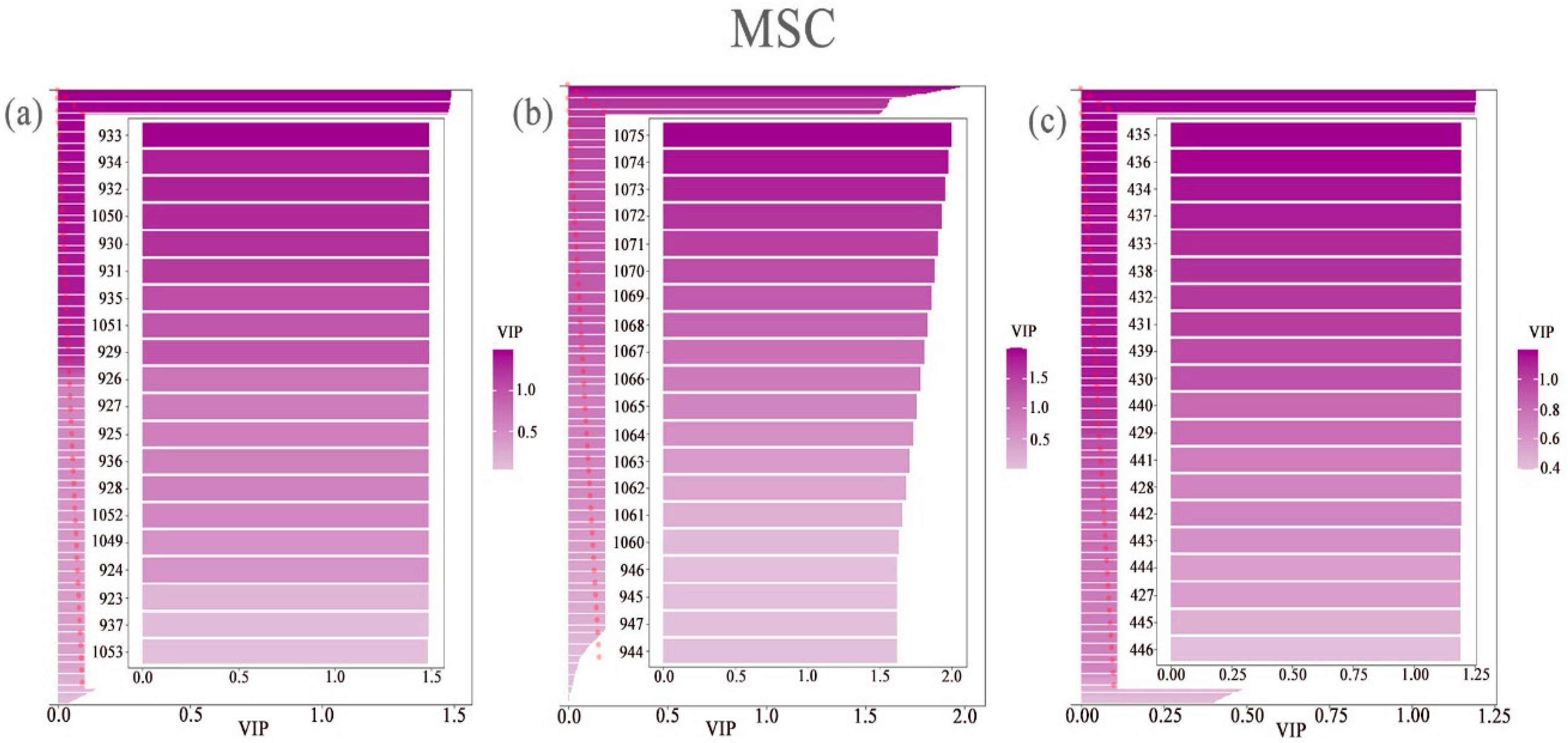
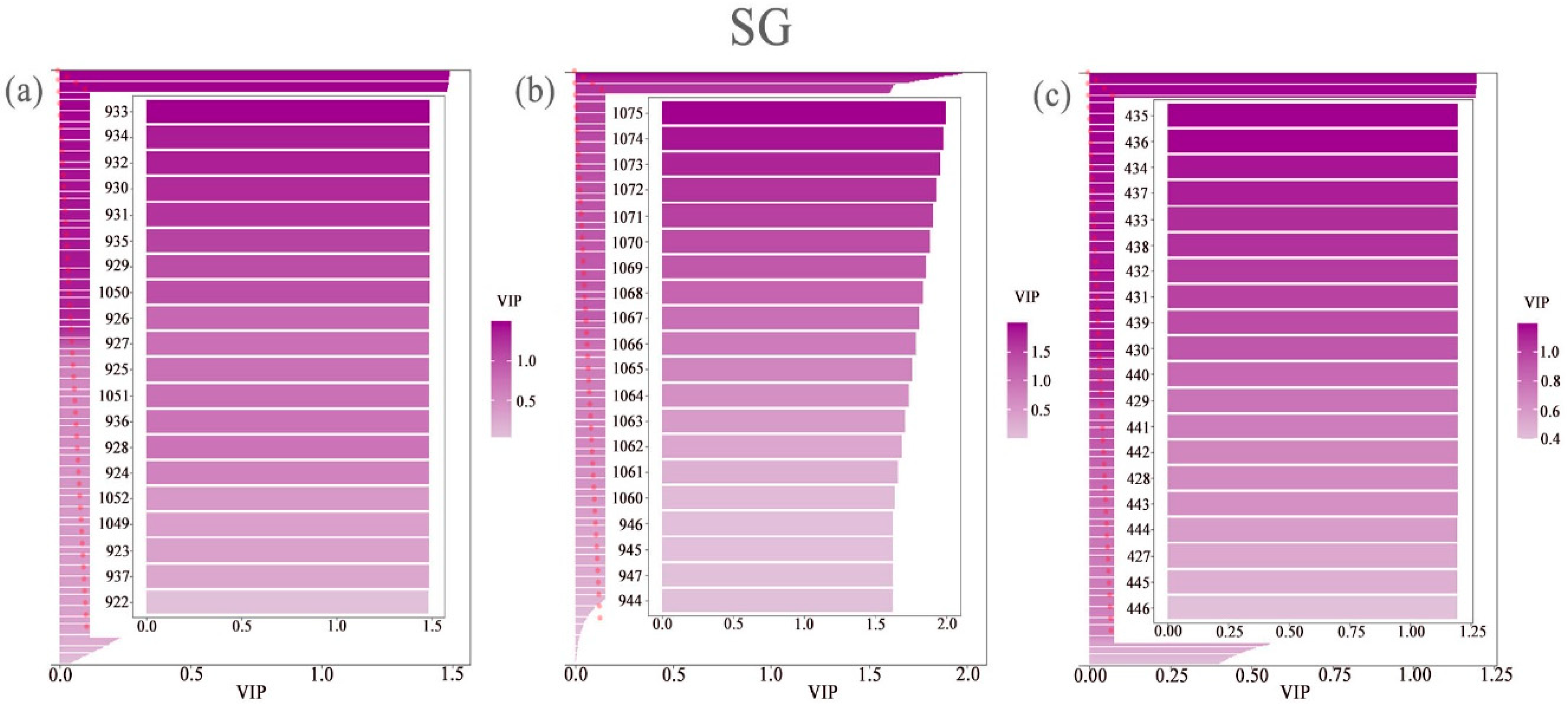
3.3. Extraction of the Spectral Reflectance of Cotton Leaves Under Different Nitrogen and Phosphorus Coupling Conditions Via PLS–DA

R 4.3.2 software was used to extract the characteristic bands of the cotton spectral data at different growth stages according to the VIP values obtained Via PLS. After FD, SNV, MSC and SG preprocessing, the characteristic bands were extracted by PLS–DA analysis, as shown in Figure 7, Figure 8, Figure 9 and Figure 10.

The feature bands selected on the basis of the PLS–VIP values greatly alleviated the complexity of the spectral data. The twenty highest VIP values were extracted at the squaring stage, initial bloom stage, peak bloom stage, initial boll stage, peak boll stage and boll opening stage, and the number of extracted feature bands (20) accounted for only 2.66% of the original spectral bands (band range 325–1075). As shown in Figure 7, Figure 8, Figure 9 and Figure 10, the results of the MSC and SG treatments based on PLS–DA were most similar. In the first component analysis, the peak bloom stage, peak boll stage, and boll opening stage were not significantly different and did not perform well. However, the FD treatment performed best throughout the growth period, followed by the SNV treatment. This shows that the original spectrum was better for FD and SNV after SG smoothing. Detailed validation values and exhaustive value listings are provided in the Supplementary Materials.

3.4. Modeling of Cotton LNCs via Hyperspectral Technology

By combining Figure 7, Figure 8, Figure 9 and Figure 10 and Table 2, the SIs with a p-value < 0.01 were combined as input vectors for modeling to construct a cotton LNCs prediction model on the basis of PLS–DA-screened feature bands. SVM and RF analysis methods were used for inversion modeling, and the data were divided into a training set and verification set to invert the cotton LNCs, as shown in

Table 3. Cotton LNC estimation model based on SVM.

Model	SP	Stage	Training Set			Validation Set
			R2	RMSE	LCCC	R2	RMSE	LCCC
SVM	FD	Squaring	0.6358	0.1250	0.3051	0.5800	0.1732	0.6979
		Initial bloom	0.9960	0.0084	0.9943	0.6270	0.1412	0.4561
		Peak bloom	0.9850	0.0073	0.9891	0.7360	0.0870	0.4290
		Initial boll	0.9777	0.0015	0.9822	0.7281	0.1168	0.4648
		Peak boll	0.6915	0.0638	0.7000	0.6318	0.0211	0.1653
		Boll opening	0.9815	0.0064	0.9670	0.6211	0.0012	0.7766
	SNV	Squaring	0.6044	0.0256	0.6188	0.5935	0.1045	0.4497
		Initial bloom	0.8901	0.1046	0.9003	0.6118	0.1695	0.7158
		Peak bloom	0.6778	0.0392	0.7191	0.6271	0.0526	0.6981
		Initial boll	0.7265	0.0054	0.6657	0.6605	0.0807	0.3650
		Peak boll	0.7127	0.0068	0.6966	0.6410	0.0620	0.6323
		Boll opening	0.5405	0.1257	0.4323	0.5579	0.0434	0.2579
	MSC	Squaring	0.9596	0.0120	0.9719	0.5059	0.0023	0.6443
		Initial bloom	0.9087	0.0396	0.9474	0.6025	0.0131	0.7245
		Peak bloom	0.5678	0.0313	0.6049	0.6099	0.0677	0.3734
		Initial boll	0.6025	0.0314	0.6863	0.6944	0.0126	0.1865
		Peak boll	0.5372	0.1246	0.5569	0.5848	0.0401	0.6055
		Boll opening	0.6589	0.2829	0.6603	0.6459	0.0957	0.5395
	SG	Squaring	0.9121	0.0138	0.9256	0.5572	0.1594	0.5931
		Initial bloom	0.9311	0.0085	0.9132	0.5790	0.0443	0.4599
		Peak bloom	0.6389	0.0158	0.7386	0.5757	0.1312	0.5850
		Initial boll	0.6903	0.0719	0.7439	0.6080	0.0093	0.3196
		Peak boll	0.5399	0.1143	0.6116	0.6290	0.0106	0.6947
		Boll opening	0.6709	0.0537	0.6179	0.6090	0.0599	0.5930
RF	FD	Squaring	0.6709	0.0562	0.6052	0.5153	0.1484	0.5373
		Initial bloom	0.8137	0.1412	0.6575	0.6036	0.1427	0.6518
		Peak bloom	0.8382	0.0023	0.7445	0.7002	0.0637	0.4286
		Initial boll	0.7720	0.1704	0.5237	0.5730	0.0589	0.7182
		Peak boll	0.7400	0.1157	0.5017	0.6444	0.0294	0.5554
		Boll opening	0.7865	0.1214	0.5110	0.6101	0.0804	0.6816
	SNV	Squaring	0.6047	0.0432	0.4451	0.5576	0.1334	0.5384
		Initial bloom	0.7810	0.0160	0.7063	0.6194	0.0486	0.7120
		Peak bloom	0.7272	0.0183	0.5269	0.6605	0.0237	0.6530
		Initial boll	0.7406	0.0534	0.5477	0.6444	0.0844	0.5421
		Peak boll	0.8003	0.0551	0.6737	0.6532	0.0846	0.6309
		Boll opening	0.6721	0.2389	0.4867	0.6027	0.0146	0.6787
	MSC	Squaring	0.7697	0.1599	0.6164	0.6848	0.0151	0.6272
		Initial bloom	0.7661	0.0193	0.7428	0.6697	0.0734	0.3307
		Peak bloom	0.6130	0.0163	0.5172	0.5719	0.0355	0.2448
		Initial boll	0.6716	0.0402	0.6047	0.6214	0.0030	0.5684
		Peak boll	0.6322	0.0130	0.6243	0.5141	0.1211	0.5907
		Boll opening	0.7051	0.0026	0.5818	0.6387	0.0186	0.3511
	SG	Squaring	0.7620	0.0434	0.7122	0.6989	0.0122	0.8213
		Initial bloom	0.7776	0.0928	0.7099	0.6097	0.0569	0.5353
		Peak bloom	0.6558	0.0008	0.5082	0.5022	0.0546	0.2203
		Initial boll	0.5888	0.1348	0.4363	0.5637	0.1058	0.3990
		Peak boll	0.5390	0.0190	0.5498	0.5149	0.0648	0.6034
		Boll opening	0.6987	0.0987	0.5627	0.5250	0.1271	0.5165

and

Table 4. Cotton LNC estimation model based on RF.

Model	SP	Stage	Training Set			Validation Set
			R2	RMSE	LCCC	R2	RMSE	LCCC
RF	FD	Squaring	0.6709	0.0562	0.6052	0.5153	0.1484	0.5373
		Initial bloom	0.8137	0.1412	0.6575	0.6036	0.1427	0.6518
		Peak bloom	0.8382	0.0023	0.7445	0.7002	0.0637	0.4286
		Initial boll	0.7720	0.1704	0.5237	0.5730	0.0589	0.7182
		Peak boll	0.7400	0.1157	0.5017	0.6444	0.0294	0.5554
		Boll opening	0.7865	0.1214	0.5110	0.6101	0.0804	0.6816
	SNV	Squaring	0.6047	0.0432	0.4451	0.5576	0.1334	0.5384
		Initial bloom	0.7810	0.0160	0.7063	0.6194	0.0486	0.7120
		Peak bloom	0.7272	0.0183	0.5269	0.6605	0.0237	0.6530
		Initial boll	0.7406	0.0534	0.5477	0.6444	0.0844	0.5421
		Peak boll	0.8003	0.0551	0.6737	0.6532	0.0846	0.6309
		Boll opening	0.6721	0.2389	0.4867	0.6027	0.0146	0.6787
	MSC	Squaring	0.7697	0.1599	0.6164	0.6848	0.0151	0.6272
		Initial bloom	0.7661	0.0193	0.7428	0.6697	0.0734	0.3307
		Peak bloom	0.6130	0.0163	0.5172	0.5719	0.0355	0.2448
		Initial boll	0.6716	0.0402	0.6047	0.6214	0.0030	0.5684
		Peak boll	0.6322	0.0130	0.6243	0.5141	0.1211	0.5907
		Boll opening	0.7051	0.0026	0.5818	0.6387	0.0186	0.3511
	SG	Squaring	0.7620	0.0434	0.7122	0.6989	0.0122	0.8213
		Initial bloom	0.7776	0.0928	0.7099	0.6097	0.0569	0.5353
		Peak bloom	0.6558	0.0008	0.5082	0.5022	0.0546	0.2203
		Initial boll	0.5888	0.1348	0.4363	0.5637	0.1058	0.3990
		Peak boll	0.5390	0.0190	0.5498	0.5149	0.0648	0.6034
		Boll opening	0.6987	0.0987	0.5627	0.5250	0.1271	0.5165

.

As shown in Table 3, the SVM model underwent four types of pretreatments, and the higher R² values and lower RMSE values were the best under the SVM–FD treatment at different growth stages. The R² values of the training set at the initial bloom stage, peak bloom stage, initial boll stage, and boll opening stage reached 0.9960, 0.9850, 0.9777, and 0.9815, respectively. The RMSE reached 0.0084, 0.0073, 0.0015, and 0.0064, and the LCCC reached 0.9943, 0.9891, 0.9822, and 0.9670, respectively. The R² value of the verification set reached 0.6270, 0.7360, 0.7281, and 0.6211; the RMSE reached 0.1412, 0.0870, 0.1168, and 0.0012; and the LCCC reached 0.4561, 0.4290, 0.4648, and 0.7766, respectively. Second, the effects of the SVM–MSC and SVM-SG treatments on the squaring stage and initial bloom stage were significant, with R² values exceeding 0.9000 and RMSE and LCCC values ranging from 0.0085 to 0.0396 and from 0.5569 to 0.9719, respectively. The R², RMSE, and LCCC values of the validation sets ranged from 0.5059 to 0.6025, 0.0023 to 0.1594, and 0.4599 to 0.7245, respectively. However, the SVM–SNV treatment did not perform well. As shown in Table 4, RF–FD also had the higher R² values and lower RMSE values. The R² values of the training sets at the initial bloom stage, peak bloom stage, initial boll stage, and boll opening stage all exceeded 0.7700, and the RMSE, and LCCC values ranged from 0.0023 to 0.1704 and from 0.5110 to 0.7445, respectively. The R², RMSE and LCCC values of the verification sets ranged from 0.5730 to 0.7002, 0.0589 to 0.1427, and 0.4286 to 0.7182, respectively. Among them, RF–SNV was more effective than the RF–MSC and RF–SG treatments, and the training set R² values were mostly above 0.7000. The RMSE and LCCC values were 0.0160–0.2389 and 0.4451–0.7063, respectively. The R², RMSE, and LCCC values of the verification sets ranged from 0.5576 to 0.6605, 0.0146 to 0.1337, and 0.5421 to 0.7120, respectively. The inversion effects of RF–MSC and RF–SG were similar.

In combination with Figure 7, Figure 8, Figure 9 and Figure 10 and Table 2, it can be seen from Table 3 and Table 4 that regardless of the use of the SVM model or the RF model, the combination of SIs and PLS–DA-extracted feature bands with a p-value < 0.01 can greatly improve the accuracy of the model [26]. Under the FD treatment in the two models, the inversion effects of the initial bloom stage, peak bloom stage, and boll opening stage with the combination of the two models were obviously better than those of the other growth stages. Under the SNV treatment, the higher R² values and lower RMSE values of the squaring stage and boll opening stage by a single characteristic band or single SI were obviously worse than those of the other growth stages combined with the two methods. The inversion results of the MSC and SG methods were similar under the two models, but the results of the SG treatment were slightly better, and the inversion results of the squaring stage and initial bloom stage were significantly better than those of the other growth stages. Combined with the higher R² values and lower RMSE values of the six growth stages of cotton, SVM–MSC in the squaring stage, SVM–FD in the initial bloom stage, SVM–FD in the peak bloom stage, SVM–FD in the initial boll stage, RF–SNV in the peak boll stage, and SVM–FD in the boll opening stage can be used as the cotton LNCs recognition models, as shown in Figure 11. According to Table 3 and Table 4, from the test effect of the model, FD showed the best performance compared with the other three treatments; the SVM model had higher R² values and lower RMSE values than the RF model.

4. Discussion

4.1. The Influence of Nitrogen-Phosphorus Coupling on LNCs in Cotton

Nitrogen and phosphorus are the key factors influencing cotton growth and leaf nitrogen concentration [54]. Reasonable nitrogen and phosphorus fertilization can significantly enhance the nitrogen absorption and yield of cotton [55]. This study shows that the effect of the nitrogen-phosphorus ratio on the nitrogen concentration of cotton leaves presents significant phased and interactive effects at different growth stages. In the early stage of cotton squaring growth, moderate application of nitrogen combined with appropriate application of phosphorus can significantly promote the absorption of nitrogen by cotton, laying a foundation for its subsequent growth. During the bloom period, a higher nitrogen level combined with a balanced phosphorus supply can further promote nitrogen accumulation, which is related to the high nutrient demand of cotton at this stage. However, during the boll stage of cotton, excessive nitrogen application inhibits further nitrogen absorption, indicating that the sensitivity of cotton to nitrogen and phosphorus varies with the growth stage. Previous studies have also shown that the interaction between nitrogen and phosphorus has a significant impact on cotton yield and nitrogen fertilizer utilization efficiency [55]. Although the application of nitrogen and phosphorus has a positive effect on cotton yield, the interaction effect between the two is not always significant. When optimizing nitrogen and phosphorus management strategies, it is necessary to take into account the nutrient requirements at different growth stages in order to maximize nitrogen absorption and yield. Therefore, in precision agriculture, fertilization strategies should be tailored to the growth stage and nutrient requirements of cotton to enhance resource utilization efficiency and crop productivity.

4.2. Potential of Spectral Pretreatment Techniques for Crop LNC Estimation

The conversion of cotton LNCs parameters via the hyperspectral technique is one of the main means used to study the nitrogen status of cotton. Original spectral data often contain noise and nonlinear features, and preprocessing can improve data quality, enhance features, reduce noise, optimize model performance, and improve analysis accuracy and efficiency [56]. Therefore, preprocessing and data transformation of the original spectrum are important steps for effectively improving the accuracy of the model. Many studies have shown that a model established using different forms of spectral transformation is better than that established using the original spectrum. This fast, simple, and easy-to-implement method mainly solves the problem of spectral collinearity through feature screening and directly builds a model by selecting wavelengths with less redundant information [57,58]. The original spectral characteristic parameters can be extracted effectively by transforming the form, and the accuracy of the model can be improved. In this study, four pretreatment methods were adopted, and PLS–DA was used to extract the characteristic parameters of the original spectrum to explore the higher R² values and lower RMSE values during different growth stages of cotton. Among them, the SVM–FD model had the highest accuracy in the four growth stages of cotton; most of the training set R² values exceeded 0.9000, the RMSE values ranged from 0.0015 to 0.1250, and the LCCC values ranged from 0.3051 to 0.9943. The R², RMSE, and LCCC values of the verification sets ranged from 0.5800 to 0.7360, 0.0012 to 0.1732, and 0.1653 to 0.7766, respectively, and the conclusion was that the FD had higher R² values and lower RMSE values, which was the best consistent with previous research results [59,60,61]. This is attributed to the fact that SVM has a stronger ability to handle nonlinear relationships and high-dimensional data than RF, especially when dealing with complex spectral data.

4.3. Advantages of Spectral Fusion in Estimating Crop LNCs

With the development of remote sensing technology, multimodal data fusion, especially hyperspectral technology fusion, has become an important research direction in many application fields, and data fusion has become a promising solution for improving model accuracy [62]. However, many studies have shown that SI monitoring of cotton leaf nitrogen content is essential for improving crop yield and quality. These SIs reflect the close relationship between nitrogen availability and the photosynthetic efficiency of cotton leaves. Higher nitrogen content usually increases chlorophyll synthesis and enhances light absorption and photosynthetic rate, which in turn affects the spectral reflectance of specific wavelength regions captured by these SIs. By analyzing the leaf reflection spectrum, the nitrogen status can be accurately evaluated, precise fertilization can be guided, fertilizer waste can be reduced, and the cost can be reduced [23,63]. Rajaei et al. [64] proposed a self-supervised spectral super-resolution (SSSR) technique for fast fusion of hyperspectral (HIS) and multispectral (MSI) images. The method estimates the spectra of high-resolution pixels from the spectra of MSI pixels by training a small deep neural network, which does not require high-resolution training data but is manually generated from the spatial degradation model of the input observed images. Therefore, this study incorporated cotton LNCs and SIs with a p-value < 0.01 to build models on the basis of the first 20 feature variables determined via PLS–DA and extracted from the original spectrum with a VIP value greater than 1. Compared with that of the RF model, the higher R² values and lower RMSE values of the SVM model in different growth stages under different pretreatments were better. This finding indicates that the SVM model performs well [65,66,67]. Moreover, combined with Figure 7, Figure 8, Figure 9 and Figure 10 and Table 2, Table 3 and Table 4, it shows that in the two models, the higher R² values and lower RMSE values of the growth period with the SIs integrated under different pretreatments were significantly better than those of the other growth periods, especially the squaring stage and initial bloom stage. This finding shows that spectral data fusion combined with PLS–DA screening of feature variables has great potential for improving the accuracy of the cotton LNCs model, especially under SVM–FD processing. Among them, the fusion model significantly improved the R², RMSE, and LCCC indicators, thus improving the accuracy of cotton LNCs inversion and contributing to the accurate and rapid monitoring of cotton LNCs, which is similar to the results of Ma et al. [68].

Compared with the research results of similar crops, the effectiveness of PRI and NDVI in estimating nitrogen status in wheat is consistent with the results of this study [69,70]. However, this study found that at different growth stages of cotton, the optimal combination of SIs and spectral bands varies. For instance, during the Peak bloom period, VOG4 and RVSI show a relatively high correlation, which may be related to the physiological characteristics of cotton at this crucial reproductive stage. This indicates that although the general principles of spectral nitrogen estimation apply to a variety of crops, to achieve the best accuracy, models tailored to specific crops and growth stages may be required.

The use of hybrid fusion technology can result in strong anti-interference ability and significantly improve the accuracy of nitrogen content inversion. Under the same algorithm framework, a fusion model is more accurate than the single data source model, especially a hybrid fusion model, which has the best performance. This proves that data fusion by combining SIs and extracted characteristic spectral bands has obvious advantages for estimating cotton LNCs. Although this study has achieved positive results, there are still some limitations. Firstly, data collection was limited to one year and one location, which might have restricted the universality of the model, as the differences in environmental conditions among different years and locations could affect the growth and spectral characteristics of cotton. Secondly, the performance of the validation set shows high variability, which may be related to insufficient sample representativeness or the model’s sensitivity to specific data features. Future research can enhance the robustness of the model by expanding the time and location range of data collection, further optimize the model to reduce the variability of validation set performance, and adjust and optimize the feature screening and model construction methods to provide guidance and new ideas for the implementation of precision agriculture.

5. Conclusions

(1)

Under the conditions of nitrogen and phosphorus coupling, cotton LNC predictions performed better under N₃P₁, N₃P₀, N₂P₂, N₂P₂, N₀P₃, and N₃P₂ at the squaring stage, initial bloom stage, peak bloom stage, initial boll stage, peak boll stage, and boll opening stage, respectively, showing a trend of first increasing and then decreasing, and the LNCs reached a maximum at the peak bloom stage.

(2)

The results revealed that SVM–MSC in the squaring stage, SVM–FD in the initial bloom stage, SVM–FD in the peak bloom stage, SVM–FD in the initial boll stage, RF–SNV in the peak boll stage, and SVM–FD in the boll opening stage could be used as LNC recognition models for cotton. FD showed the best performance compared with the other three treatments, and the SVM model had a higher R² value and lower RMSE value than the RF model.

References

1. Dai, J.; Kong, X.; Zhang, D.; Li, W.; Dong, H. Technologies and theoretical basis of light and simplified cotton cultivation in China. Field Crops Res. 2017, 214, 142–148. [Google Scholar] [CrossRef]
2. Ata-Ul-Karim, S.T.; Cang, L.; Wang, Y.; Zhou, D. Effects of soil properties, nitrogen application, plant phenology, and their interactions on plant uptake of cadmium in wheat. J. Hazard. Mater. 2020, 384, 121452. [Google Scholar] [CrossRef]
3. Ma, J.; He, P.; Xu, X.; He, W.; Liu, Y.; Yang, F.; Chen, F.; Li, S.; Tu, S.; Jin, J.; et al. Temporal and spatial changes in soil available phosphorus in China (1990–2012). Field Crops Res. 2016, 192, 13–20. [Google Scholar] [CrossRef]
4. Lemercier, B.; Gaudin, L.; Walter, C.; Aurousseau, P.; Arrouays, D.; Schvartz, C.; Saby, N.P.A.; Follain, S.; Abrassart, J. Soil phosphorus monitoring at the regional level by means of a soil test database. Soil Use Manag. 2008, 24, 131–138. [Google Scholar] [CrossRef]
5. Sonobe, R.; Hirono, Y. Carotenoid Content Estimation in Tea Leaves Using Noisy Reflectance Data. Remote Sens. 2023, 15, 4303. [Google Scholar] [CrossRef]
6. Falcioni, R.; Antunes, W.C.; Demattê, J.A.M.; Nanni, M.R. A Novel Method for Estimating Chlorophyll and Carotenoid Concentrations in Leaves: A Two Hyperspectral Sensor Approach. Sensors 2023, 23, 3843. [Google Scholar] [CrossRef]
7. Yang, Z.; Tian, J.; Zhang, L.; Zan, O.; Yan, X.; Feng, K. Spectral detection of leaf carbon and nitrogen as a proxy for remote assessment of photosynthetic capacity for wheat and maize under nitrogen stress. Comput. Electron. Agric. 2024, 224, 109174. [Google Scholar] [CrossRef]
8. Li, D.; Hu, Q.; Zhang, J.; Dian, Y.; Hu, C.; Zhou, J. Leaf Nitrogen and Phosphorus Variation and Estimation of Citrus Tree under Two Labor-Saving Cultivation Modes Using Hyperspectral Data. Remote Sens. 2024, 16, 3261. [Google Scholar] [CrossRef]
9. Li, J.; Shi, L.; Mo, X.; Hu, X.; Su, C.; Han, J.; Deng, X.; Du, S.; Li, S. Self-correcting deep learning for estimating rice leaf nitrogen concentration with mobile phone images. Comput. Electron. Agric. 2024, 227, 109497. [Google Scholar] [CrossRef]
10. Hu, W.; Tang, W.; Li, C.; Wu, J.; Liu, H.; Wang, C.; Luo, X.; Tang, R. Handling the Challenges of Small-Scale Labeled Data and Class Imbalances in Classifying the N and K Statuses of Rubber Leaves Using Hyperspectroscopy Techniques. Plant Phenomics 2024, 6, 0154. [Google Scholar] [CrossRef] [PubMed]
11. Furlanetto, R.H.; Crusiol, L.G.T.; Gonçalves, J.V.F.; Nanni, M.R.; Junior, A.d.O.; de Oliveira, F.A.; Sibaldelli, R.N.R. Machine learning as a tool to predict potassium concentration in soybean leaf using hyperspectral data. Precis. Agric. 2023, 24, 2264–2292. [Google Scholar] [CrossRef]
12. Jin, X.; Xu, L.; Feng, H.; Wang, K.; Niu, J.; Su, X.; Chen, L.; Zheng, H.; Huang, J. Optimizing Multidimensional Spectral Indices and Ensemble Learning Methods for Estimating Nitrogen Content in Torreya grandis Leaves Based on UAV Hyperspectral. Forests 2024, 16, 40. [Google Scholar] [CrossRef]
13. Wang, J.; Li, Z.; Jin, X.; Liang, G.; Struik, P.C.; Gu, J.; Zhou, Y. Phenotyping flag leaf nitrogen content in rice using a three-band spectral index. Comput. Electron. Agric. 2019, 162, 475–481. [Google Scholar] [CrossRef]
14. Yang, S.; Li, J.; Li, J.; Zhang, X.; Ma, C.; Liu, Z.; Ren, M. Estimating the Canopy Nitrogen Content in Maize by Using the Transform-Based Dynamic Spectral Indices and Random Forest. Sustainability 2024, 16, 8011. [Google Scholar] [CrossRef]
15. Wang, J.; Wang, H.; Tian, T.; Cui, J.; Shi, X.; Song, J.; Li, T.; Li, W.; Zhong, M.; Zhang, W. Construction of spectral index based on multi-angle spectral data for estimating cotton leaf nitrogen concentration. Comput. Electron. Agric. 2022, 201, 107328. [Google Scholar] [CrossRef]
16. Lu, M.; Wang, H.; Xu, J.; Wei, Z.; Li, Y.; Hu, J.; Tian, S. A Vis/NIRS device for evaluating leaf nitrogen content using K-means algorithm and feature extraction methods. Comput. Electron. Agric. 2024, 225, 109301. [Google Scholar] [CrossRef]
17. Tan, J.; Ding, J.; Wang, Z.; Han, L.; Wang, X.; Li, Y.; Zhang, Z.; Meng, S.; Cai, W.; Hong, Y. Estimating soil salinity in mulched cotton fields using UAV-based hyperspectral remote sensing and a Seagull Optimization Algorithm-Enhanced Random Forest Model. Comput. Electron. Agric. 2024, 221, 109017. [Google Scholar] [CrossRef]
18. Yang, H.; Yin, H.; Li, F.; Hu, Y.; Yu, K. Machine learning models fed with optimized spectral indices to advance crop nitrogen monitoring. Field Crops Res. 2023, 293, 108844. [Google Scholar] [CrossRef]
19. Qin, S.; Ding, Y.; Zhou, T.; Zhai, M.; Zhang, Z.; Fan, M.; Lv, X.; Zhang, Z.; Zhang, L. “Image-Spectral” fusion monitoring of small cotton samples nitrogen content based on improved deep forest. Comput. Electron. Agric. 2024, 221, 109002. [Google Scholar] [CrossRef]
20. Sun, Q.; Gu, X.; Chen, L.; Qu, X.; Zhang, S.; Zhou, J.; Pan, Y. Hyperspectral estimation of maize (Zea mays L.) yield loss under lodging stress. Field Crops Res. 2023, 302, 109042. [Google Scholar] [CrossRef]
21. Wang, J.; Tian, T.; Wang, H.; Cui, J.; Zhu, Y.; Zhang, W.; Tong, X.; Zhou, T.; Yang, Z.; Sun, J. Estimating cotton leaf nitrogen by combining the bands sensitive to nitrogen concentration and oxidase activities using hyperspectral imaging. Comput. Electron. Agric. 2021, 189, 106390. [Google Scholar] [CrossRef]
22. Flynn, K.C.; Witt, T.W.; Baath, G.S.; Chinmayi, H.K.; Smith, D.R.; Gowda, P.H.; Ashworth, A.J. Hyperspectral reflectance and machine learning for multi-site monitoring of cotton growth. Smart Agric. Technol. 2024, 9, 100536. [Google Scholar] [CrossRef]
23. Yin, C.; Lv, X.; Zhang, L.; Ma, L.; Wang, H.; Zhang, L.; Zhang, Z. Hyperspectral UAV Images at Different Altitudes for Monitoring the Leaf Nitrogen Content in Cotton Crops. Remote Sens. 2022, 14, 2576. [Google Scholar] [CrossRef]
24. Shu, M.; Zhu, J.; Yang, X.; Gu, X.; Li, B.; Ma, Y. A spectral decomposition method for estimating the leaf nitrogen status of maize by UAV-based hyperspectral imaging. Comput. Electron. Agric. 2023, 212, 108100. [Google Scholar] [CrossRef]
25. Chen, R.; Liu, W.; Yang, H.; Jin, X.; Yang, G.; Zhou, Y.; Zhang, C.; Han, S.; Meng, Y.; Zhai, C.; et al. A novel framework to assess apple leaf nitrogen content: Fusion of hyperspectral reflectance and phenology information through deep learning. Comput. Electron. Agric. 2024, 219, 108816. [Google Scholar] [CrossRef]
26. Shao, Y.; Yang, W.; Wang, J.; Lu, Z.; Zhang, M.; Chen, D. Cotton Disease Recognition Method in Natural Environment Based on Convolutional Neural Network. Agriculture 2024, 14, 1577. [Google Scholar] [CrossRef]
27. Aierken, N.; Yang, B.; Li, Y.; Jiang, P.; Pan, G.; Li, S. A review of unmanned aerial vehicle based remote sensing and machine learning for cotton crop growth monitoring. Comput. Electron. Agric. 2024, 227, 109601. [Google Scholar] [CrossRef]
28. Karmakar, P.; Teng, S.W.; Murshed, M.; Pang, S.; Li, Y.; Lin, H. Crop monitoring by multimodal remote sensing: A review. Remote Sens. Appl. Soc. Environ. 2024, 33, 101093. [Google Scholar] [CrossRef]
29. Stein, M.; Bargoti, S.; Underwood, J. Image Based Mango Fruit Detection, Localisation and Yield Estimation Using Multiple View Geometry. Sensors 2016, 16, 1915. [Google Scholar] [CrossRef]
30. Savitzky, A.; Golay, M.J.E. Smoothing and Differentiation of Data by Simplified Least Squares Procedures. Anal. Chem. 1964, 36, 1627–1639. [Google Scholar] [CrossRef]
31. Chong, I.; Jun, C. Performance of some variable selection methods when multicollinearity is present. Chemom. Intell. Lab. Syst. 2004, 78, 103–112. [Google Scholar] [CrossRef]
32. Montero, D.; Aybar, C.; Mahecha, M.D.; Martinuzzi, F.; Söchting, M.; Wieneke, S. A standardized catalogue of spectral indices to advance the use of remote sensing in Earth system research. Sci. Data 2023, 10, 197. [Google Scholar] [CrossRef]
33. Richardson, A.J.; Wiegand, A. Distinguishing vegetation from soil background information. Photogramm. Eng. Remote Sens. 1977, 43, 1541–1552. [Google Scholar]
34. Sims, D.A.; Gamon, J.A. Relationships between leaf pigment content and spectral reflectance across a wide range of species, leaf structures and developmental stages. Remote Sens. Environ. 2002, 81, 337–354. [Google Scholar] [CrossRef]
35. Gamon, J.A.; Peñuelas, J.; Field, C.B. A narrow-waveband spectral index that tracks diurnal changes in photosynthetic efficiency. Remote Sens. Environ. 1992, 41, 35–44. [Google Scholar] [CrossRef]
36. Dash, J.; Curran, P.J. The MERIS terrestrial chlorophyll index. Int. J. Remote Sens. 2004, 25, 5403–5413. [Google Scholar] [CrossRef]
37. Rondeaux, G.; Steven, M.; Baret, F. Optimization of soil-adjusted vegetation index. Remote Sens. Environ. 1996, 24, 109–127. [Google Scholar] [CrossRef]
38. Haboudane, D.; Miller, J.R.; Tremblay, N.; Zarco-Tejada, P.J.; Dextraze, L. Integrated narrow-band vegetation indices for prediction of crop chlorophyll content for application to precision agriculture. Remote Sens. Environ. 2002, 81, 416–426. [Google Scholar] [CrossRef]
39. Gitelson, A.; Merzlyak, M.N. Spectral Reflectance Changes Associated with Autumn Senescence of Aesculus hippocastanum L. and Acer platanoides L. Leaves. Spectral Features and Relation to Chlorophyll Estimation. J. Plant Physiol. 1994, 143, 286–292. [Google Scholar] [CrossRef]
40. Zarco-Tejada, P.J.; Miller, J.R.; Noland, T.L.; Mohammed, G.H.; Sampson, P.H. Scaling-up and model inversion methods with narrowband optical indices for chlorophyll content estimation in closed forest canopies with hyperspectral data. IEEE Trans. Geosci. Remote Sens. 2001, 39, 1491–1507. [Google Scholar] [CrossRef]
41. Wang, F.; Yan, Z.; Zhao, X.; Guo, X.; Zhou, Y.; Guo, J. Parameter selection of partial least squares model for hyperspectral estimation of chlorophyll content in camellia oleifera leaves. Acta Agric. Univ. Jiangxiensis 2022, 44, 86–96. [Google Scholar] [CrossRef]
42. Schlerf, M.; Atzberger, C.; Hill, J. Remote sensing of forest biophysical variables using HyMap imaging spectrometer data. Remote Sens. Environ. 2004, 95, 177–194. [Google Scholar] [CrossRef]
43. Liang, L.; Di, L.; Zhang, L.; Deng, M.; Qin, Z.; Zhao, S.; Lin, H. Estimation of crop LAI using hyperspectral vegetation indices and a hybrid inversion method. Remote Sens. Environ. 2015, 165, 123–134. [Google Scholar] [CrossRef]
44. Hong, S.; Zhang, Z.; Zhang, L.; Ma, L.; Hai, X.; Wang, Z.; Zhang, H.; Lv, X. Hyperspectral estimation model of chlorophyll content in cotton canopy leaves under drip irrigation at different growths. Cotton Sci. 2019, 31, 138–146. [Google Scholar] [CrossRef]
45. Fu, K.; Zhang, W.; Cao, H.; Zhu, Y.; Waili, S.; Zhang, W.; Feng, C. Research progress on crop diseases and insect pests monitoring based on spectrum. J. Agric. Sci. Technol. 2014, 16, 90–98. [Google Scholar] [CrossRef]
46. Sun, L.; Cheng, L. Analysis of spectral response of vegetation leaf biochemical components. Spectrosc. Spectr. Anal. 2010, 30, 3031–3035. [Google Scholar] [CrossRef]
47. Chen, S.; Chen, Y.; Ren, F.; Zheng, Y. Estimation of maize chlorophyll content based on spectral index. J. Xinyang Norm. Univ. Nat. Sci. Ed. 2021, 34, 225–229. [Google Scholar]
48. Naidu, R.A.; Perry, E.M.; Pierce, F.J.; Mekuria, T. The potential of spectral reflectance technique for the detection of Grapevine leafroll-associated virus-3 in two red-berried wine grape cultivars. Comput. Electron. Agric. 2009, 66, 38–45. [Google Scholar] [CrossRef]
49. Mahlein, A.-K.; Rumpf, T.; Welke, P.; Dehne, H.-W.; Plümer, L.; Steiner, U.; Oerke, E.-C. Development of spectral indices for detecting and identifying plant diseases. Remote Sens. Environ. 2013, 128, 21–30. [Google Scholar] [CrossRef]
50. Liu, L.; Huang, W.; Pu, R.; Wang, J. Detection of Internal Leaf Structure Deterioration Using a New Spectral Ratio Index in the Near-Infrared Shoulder Region. J. Integr. Agric. 2014, 13, 760–769. [Google Scholar] [CrossRef]
51. Hong, Y.; Liu, Y.; Chen, Y.; Liu, Y.; Yu, L.; Liu, Y.; Cheng, H. Application of fractional-order derivative in the quantitative estimation of soil organic matter content through visible and near-infrared spectroscopy. Geoderma 2019, 337, 758–769. [Google Scholar] [CrossRef]
52. Breiman, L. Random Forests. Mach. Learn. 2001, 45, 5–32. [Google Scholar] [CrossRef]
53. Lin, L.I.-K. A concordance correlation coefficient to evaluate reproducibility. Biometrics 1989, 45, 255–268. [Google Scholar] [CrossRef]
54. Peng, L.; Xin, N.; Lv, X.; Li, N.; Li, F.; Geng, L.; Chen, H.; Lai, N. Inversion of nitrogen and phosphorus contents in cotton leaves based on the Gaussian mixture model and differences in hyperspectral features of UAV. Spectrochim. Acta Part A Mol. Biomol. Spectrosc. 2025, 327, 125419. [Google Scholar] [CrossRef]
55. Luo, H.; Wang, Q.; Zhang, J.; Wang, L.; Li, Y.; Yang, G. Minimum fertilization at the appearance of the first flower benefits cotton nutrient utilization of nitrogen, phosphorus and potassium. Sci. Rep. 2020, 10, 6815. [Google Scholar] [CrossRef]
56. Arneberg, R.; Rajalahti, T.; Flikka, K.; Berven, F.S.; Kroksveen, A.C.; Berle, M.; Myhr, K.M.; Vedeler, C.A.; Ulvik, R.J.; Kvalheim, O.M. Pretreatment of mass spectral profiles: Application to proteomic data. Anal. Chem. 2007, 79, 7014–7026. [Google Scholar] [CrossRef]
57. Nguyen, T.H.; Lee, B. Assessment of rice leaf growth and nitrogen status by hyperspectral canopy reflectance and partial least square regression. Eur. J. Agron. 2006, 24, 349–356. [Google Scholar] [CrossRef]
58. Li, L.; Lu, J.; Wang, S.; Ma, Y.; Wei, Q.; Li, X.; Cong, R.; Ren, T. Methods for estimating leaf nitrogen concentration of winter oilseed rape (Brassica napus L.) using in situ leaf spectroscopy. Ind. Crops Prod. 2016, 91, 194–204. [Google Scholar] [CrossRef]
59. Liu, L.; Wang, J.; Bian, H.; Abdalla, A.N. Near-Infrared Spectroscopy Combined With Support Vector Machine Model to Realize Quality Control of Ginkgolide Production. IEEE Photonics J. 2024, 16, 6600608. [Google Scholar] [CrossRef]
60. Chen, D.; Chen, Y.; Xue, D. 1-D and 2-D digital fractional-order Savitzky–Golay differentiator. Signal Image Video Process. 2012, 6, 503–511. [Google Scholar] [CrossRef]
61. Hong, Y.; Chen, Y.; Yu, L.; Liu, Y.; Liu, Y.; Zhang, Y.; Liu, Y.; Cheng, H. Combining Fractional Order Derivative and Spectral Variable Selection for Organic Matter Estimation of Homogeneous Soil Samples by VIS–NIR Spectroscopy. Remote Sens. 2018, 10, 479. [Google Scholar] [CrossRef]
62. Kahraman, S.; Bacher, R. A comprehensive review of hyperspectral data fusion with LIDAR and SAR data. Annu. Rev. Control. 2021, 51, 236–253. [Google Scholar] [CrossRef]
63. Liu, Y.; Chen, Y.; Wen, M.; Lu, Y.; Ma, F. Accuracy Comparison of Estimation on Cotton Leaf and Plant Nitrogen Content Based on UAV Digital Image under Different Nutrition Treatments. Agronomy 2023, 13, 1686. [Google Scholar] [CrossRef]
64. Rajaei, A.; Abiri, E.; Helfroush, M.S. Self-supervised spectral super-resolution for a fast hyperspectral and multispectral image fusion. Sci. Rep. 2024, 14, 29820. [Google Scholar] [CrossRef] [PubMed]
65. Yu, P.; Yang, T.; Chen, S.; Kuo, C.; Tseng, H.W. Comparison of random forests and support vector machine for real-time radar-derived rainfall forecasting. J. Hydrol. 2017, 552, 92–104. [Google Scholar] [CrossRef]
66. Abe, B.T.; Olugbara, O.O.; Marwala, T. Experimental comparison of support vector machines with random forests for hyperspectral image land cover classification. J. Earth Syst. Sci. 2014, 123, 779–790. [Google Scholar] [CrossRef]
67. Bawa, A.; Samanta, S.; Himanshu, S.K.; Singh, J.; Kim, J.J.; Zhang, T.; Chang, A.; Jung, J.; DeLaune, P.; Bordovsky, J.; et al. A support vector machine and image processing based approach for counting open cotton bolls and estimating lint yield from UAV imagery. Smart Agric. Technol. 2023, 3, 100140. [Google Scholar] [CrossRef]
68. Ma, Y.; Chen, H.; Zhao, G.; Wang, Z.; Wang, D. Spectral Index Fusion for Salinized Soil Salinity Inversion Using Sentinel-2A and UAV Images in a Coastal Area. IEEE Access 2020, 8, 159595–159608. [Google Scholar] [CrossRef]
69. Guan, S.; Fukami, K.; Matsunaka, H.; Okami, M.; Tanaka, R.; Nakano, H.; Sakai, T.; Nakano, K.; Ohdan, H.; Takahashi, K. Assessing Correlation of High-Resolution NDVI with Fertilizer Application Level and Yield of Rice and Wheat Crops Using Small UAVs. Remote Sens. 2019, 11, 112. [Google Scholar] [CrossRef]
70. Sultana, R.S.; Ali, A.; Ahmad, A.; Mubeen, M.; Zia-Ul-Haq, M.; Ahmad, S.; Ercisli, S.; Jaafar, Z.E.H. Normalized Difference Vegetation Index as a Tool for Wheat Yield Estimation: A Case Study from Faisalabad, Pakistan. Sci. World J. 2014, 2014, 725326. [Google Scholar] [CrossRef]
Figure 1. Overview of the study area. (a) Map of China; (b) Xinjiang Uygur Autonomous Region; (c) Aral reclamation area; and (d) Test plot.
Agronomy 15 01701 g001
Figure 2. Cotton LNC changes under different nitrogen and phosphorus coupling conditions at different growth stages. (af) represent the squaring stage, initial bloom stage, peak bloom stage, initial boll stage, peak boll stage, and boll opening stage, respectively. Different colors mainly distinguish the amount of phosphorus applied, while the same color from left to right mainly distinguishes the amount of nitrogen applied.
Agronomy 15 01701 g002
Figure 3. Thermal map analysis of cotton LNCs and SIs based on FD at different growth stages. (af) represent the squaring stage, initial bloom stage, peak bloom stage, initial boll stage, peak boll stage, and boll opening stage, respectively.
Agronomy 15 01701 g003
Figure 4. Thermal map analysis of cotton LNCs and SIs based on SNV at different growth stages. (af) represent the squaring stage, initial bloom stage, peak bloom stage, initial boll stage, peak boll stage, and boll opening stage, respectively.
Agronomy 15 01701 g004
Figure 5. Thermal map analysis of cotton LNCs and SIs on the basis of MSC at different growth stages. (af) represent the squaring stage, initial bloom stage, peak bloom stage, initial boll stage, peak boll stage, and boll opening stage, respectively.
Agronomy 15 01701 g005
Figure 6. Thermal map analysis of cotton LNCs and SIs on the basis of SG at different growth stages. (af) represent the squaring stage, initial bloom stage, peak bloom stage, initial boll stage, peak boll stage, and boll opening stage, respectively.
Agronomy 15 01701 g006
Figure 7. PLS–DA of the spectral reflectance of cotton leaves subjected to FD at different growth stages. (af) represent the squaring stage, initial bloom stage, peak bloom stage, initial boll stage, peak boll stage, and boll opening stage, respectively.
Agronomy 15 01701 g007
Figure 8. PLS–DA of the spectral reflectance of cotton leaves subjected to SNV at different growth stages. (ae) represent the squaring stage, initial bloom stage, peak bloom stage, initial boll stage, and peak boll stage, respectively.
Agronomy 15 01701 g008
Figure 9. PLS–DA of the spectral reflectance of the cotton leaves subjected to MSC at different growth stages. (ac) represent the squaring stage, initial bloom stage, and initial boll stage, respectively.
Agronomy 15 01701 g009
Figure 10. PLS–DA of the spectral reflectance of the cotton leaves subjected to SG at different growth stages. (ac) represent the squaring stage, initial bloom stage, and initial boll stage, respectively.
Agronomy 15 01701 g010
Figure 11. Fitting diagram of optimal training and verification based on machine learning. (af) represent the squaring stage, initial bloom stage, peak bloom stage, initial boll stage, peak boll stage, and boll opening stage, respectively. Two lines of different colors respectively represent the fitting lines of the training set (blue) and the validation set (red).
Agronomy 15 01701 g011