SWMD-YOLO: A Lightweight Model for Tomato Detection in Greenhouse Environments

Abstract

The accurate detection of occluded tomatoes in complex greenhouse environments remains challenging due to the limited feature representation ability and high computational costs of existing models. This study proposes SWMD-YOLO, a lightweight multi-scale detection network optimized for greenhouse scenarios. The model integrates switchable atrous convolution (SAConv) and wavelet transform convolution (WTConv) for the dynamic adjustment of receptive fields for occlusion-adaptive feature extraction and to decompose features into multi-frequency sub-bands, respectively, thus preserving critical edge details of obscured targets. Traditional down-sampling is replaced with a dynamic sample (DySample) operator to minimize information loss during resolution transitions, while a multi-scale convolutional attention (MSCA) mechanism prioritizes discriminative regions under varying illumination. Additionally, we introduce Focaler-IoU, a novel loss function that addresses sample imbalance by dynamically re-weighting gradients for partially occluded and multi-scale targets. Experiments on greenhouse tomato data sets demonstrate that SWMD-YOLO achieves 93.47% mAP50 with a detection speed of 75.68 FPS, outperforming baseline models in accuracy while reducing parameters by 18.9%. Cross-data set validation confirms the model’s robustness to complex backgrounds and lighting variations. Overall, the proposed model provides a computationally efficient solution for real-time crop monitoring in resource-constrained precision agriculture systems.

1. Introduction

Tomato is one of the most widely grown vegetables in Chinese agriculture. China is not only a global leader in tomato production, but also a major exporter of tomatoes [1,2,3,4,5,6,7,8,9,10,11,12,13,14,15,16,17]. While harvesting tomatoes by hand is labor- and time-intensive, mechanized harvesting not only reduces labor costs but also increases harvesting efficiency [10]. In this context, the harvesting robot first utilizes a computer vision system to detect the tomato fruit, and then guides a robotic arm to perform the harvesting operation based on the detection results [18,19,20,21,22,23]. Therefore, fruit detection is a key component of the harvesting process, and its accuracy and speed directly affect the efficiency of harvesting using a robot [24,25,26,27]. However, tomato fruits may exhibit different growth poses, overlap each other, and/or be heavily shaded by leaves, branches, and stems, which poses a challenge for their recognition by a robot. The fast and accurate recognition of tomato fruits in complex greenhouse environments is a pressing issue in the development of tomato picking robots.

In recent years, deep learning technology—especially single-stage algorithms—has become a promising solution for the real-time and efficient detection of tomatoes. YOLO (“you only look once”) series networks [28,29,30,31,32,33,34,35,36,37,38,39] and other single-stage algorithms like SSD and RetinaNet have attracted considerable attention due to their fast processing time and high accuracy, which make them suitable for precision agriculture applications.

For instance, Li et al. (2021) [40] employed a YOLOv4 model for tomato detection, achieving an impressive average precision (AP) of 0.86 in a greenhouse environment; however, despite its high accuracy, the model struggled to detect smaller tomatoes and exhibited reduced performance under varying lighting conditions. Similarly, Zhang et al. (2023) [41] implemented a YOLOv5 model for tomato detection, achieving a high detection accuracy of 91.2%; however, the model showed limitations when dealing with overlapping tomatoes and complex backgrounds. Further improvements were made by Gao et al. (2024) [42], who combined a YOLOv5 model with transfer learning to detect tomatoes in dynamic environments, yielding an accuracy of 93.6%. While their method showed robust performance across varying conditions, it struggled in terms of its real-time application due to the computational load required for large-scale data sets. On the other hand, Wang et al. (2021) [43] explored the RetinaNet model, achieving a remarkable precision of 90.3%. However, this approach was less effective in situations where the tomatoes were heavily occluded by leaves or other plants, making it less reliable in dense cropping scenes. Moreover, Cardellicchio et al. (2023) [44] proposed a single-stage model using an improved Faster R-CNN architecture tailored for tomato detection, which achieved an AP score of 92.5%. However, the model faced challenges in terms of speed and was unsuitable for applications requiring high real-time performance in large fields. Similarly, Zhu et al. (2021) [45] tested a single-stage detection model that yielded a precision of 89.1%, but it struggled in terms of detection accuracy when the tomatoes presented irregular patterns within the field. This limitation makes it less effective for large-scale industrial applications that require flexibility and scalability. Cai et al. (2024) [39] proposed an improved YOLOv7-tiny model for the detection of cherry tomatoes in greenhouse environments, incorporating multi-modal RGB-D perception to enhance the precision of detection and real-time performance. While their method achieved a precision of 88.1% for the detection of cherry tomatoes, the model was found to struggle with handling complex background interference and the occlusion of tomatoes in dense clusters. In scenarios where the tomatoes are heavily overlapped, the detection accuracy dropped by 5–10%, especially in environments with varying lighting conditions. Yang et al. (2024) [46] developed an improved YOLOv8 model for tomato ripeness recognition, integrating the RCA-CBAM attention module and BiFPN to better capture the color of and size variations in tomatoes at different ripening stages. This model achieved a precision of 95.8% and an accuracy of 91.7%, but its real-time processing capabilities were found to be limited. In real-world testing, the model’s inference time was 120 ms per image, which is too slow for applications requiring real-time decision-making, particularly when large numbers of tomatoes are present in the frame. Sun et al. (2024) [47] proposed the S-YOLO model, a lightweight detection model based on YOLOv8s, focusing on improving the detection accuracy for occluded and small tomatoes in greenhouse settings. The model achieved an impressive 92.46% mAP and a detection speed of 74.05 FPS. However, its performance dropped when exposed to highly variable lighting conditions, with the model’s accuracy decreasing by as much as 7% in low-light environments; furthermore, it struggled to detect extremely small tomatoes or those that are partially hidden behind dense foliage.

From the above literature it can be concluded that, despite the progress made in single-stage deep learning methods for tomato detection, several challenges remain. Issues such as detecting small or occluded tomatoes, handling varying lighting conditions, and real-time performance on large-scale data sets remain to be addressed. The majority of existing models also struggle when faced with high-density environments or complex backgrounds, limiting their practicality in certain agricultural settings.

In conclusion, although existing object detection algorithms have demonstrated remarkable progress in agricultural applications, significant challenges persist in addressing complex greenhouse environments characterized by occlusions, varying illumination, and intricate backgrounds. Existing methods often struggle to balance computational efficiency with the ability to capture the fine-grained details of small and overlapping targets, such as tomatoes in dense foliage. While YOLO-based architectures have emerged as efficient solutions for real-time detection, their performance in terms of handling occlusion and multi-scale features remains sub-optimal in resource-constrained settings. Moreover, the computational overhead incurred by the use of many advanced modules limits their practicality for deployment on the embedded systems commonly employed in the context of smart agriculture.

To address these challenges, this study presents SWMD-YOLO: a lightweight and robust tomato detection model based on an enhanced YOLO11 architecture. Through integrating novel modules for multi-scale feature extraction and adaptive fusion, SWMD-YOLO achieves superior accuracy and real-time performance in greenhouse environments. The primary contributions of this work are as follows:

1. Enhanced multi-scale feature extraction: A hybrid backbone network is proposed, combining switchable atrous convolution (SAConv) and wavelet transform convolution (WTConv). SAConv dynamically adjusts receptive fields to capture both local and global contextual information, while WTConv decomposes features into multi-frequency sub-bands using Haar wavelets, enhancing the model’s ability to discern the fine details and edges of occluded tomatoes. This dual mechanism significantly improves the robustness of detection in cluttered scenes.

2. Dynamic feature fusion with adaptive sampling: Traditional down-sampling operations are replaced with a dynamic sample (DySample) operator in the neck of the network. DySample employs learnable weights to adaptively up-sample and fuse multi-scale features, minimizing information loss during resolution transitions. This module ensures the precise localization of small targets while maintaining computational efficiency.

3. Context-aware attention mechanism: A multi-scale convolutional attention (MSCA) module is introduced to refine feature representations. By aggregating multi-scale contextual cues and dynamically re-weighting critical regions, MSCA suppresses background noise and emphasizes discriminative tomato features, further enhancing the detection accuracy under illumination variations and partial occlusions.

4. Improved loss function: Traditional bounding box regression loss functions (e.g., IoU, GIoU, SIoU) focus primarily on spatial alignment between predicted and ground truth boxes, but overlook the impact of the target’s morphology on the regression accuracy. To address this, we propose Focaler-IoU, a loss function that dynamically adjusts the weights of difficult and easy samples, thus enhancing detection accuracy—especially for small or occluded targets—in the tomato detection task.

This paper is structured as follows: Section 1 reviews the evolution of object detection algorithms, focusing on challenges particular to agricultural applications. Section 2 details the design of the SWMD-YOLO network, including its core components and training strategies. Section 3 details the evaluation of the model’s performance through comparative experiments and ablation studies, highlighting its advantages over state-of-the-art methods. Finally, Section 4 discusses the implications of the presented findings and outlines future research directions.

2. Materials and Methods

This study presents a lightweight detection network named SWMD-YOLO, an enhanced architecture developed based on YOLO11, which is specifically optimized for the efficient detection of tomatoes in greenhouse environments. The proposed model strategically balances computational efficiency and detection accuracy through three key architectural innovations. First, the backbone network is enhanced by replacing its standard convolution modules with SAConv and WTConv. This dual-branch design strengthens the model’s multi-scale feature extraction capabilities while maintaining a lightweight structure, enabling it to robustly handle the occlusions and multi-scale variations which are typical of dense tomato clusters. Second, the conventional down-sampling operations in both the backbone and neck networks are replaced with a dynamic up-sampling operator (DySample), which minimizes information loss during resolution reduction and improves the model’s feature representation ability, ensuring high-resolution feature retention even under complex lighting conditions. Third, the MSCA module is embedded into the neck network to refine the fusion of features through the adaptive weighting of critical spatial and channel information. As illustrated in Figure 1, these innovations collectively enable SWMD-YOLO to achieve high-precision tomato detection with reduced computational complexity, making it well suited for deployment in the context of greenhouse robotic harvesting.

In YOLOV11, traditional C2f modules are replaced with the C3k2 module, which leverages parallel convolutional branches (splitting input feature maps to process shallow and deep features separately) and variable kernel sizes (e.g., 3 × 3, 5 × 5) for efficient feature fusion, significantly improving its detection accuracy in complex scenes and small objects. The C2PSA module integrates CSP structures with pyramid slice attention (PSA), using multi-scale convolutional kernels and SE channel weighting to dynamically enhance the perception of critical regions, thus achieving a 50% reduction in computational costs. A dedicated tiny-object detection head (P2 layer) further optimizes its multi-scale detection ability. For training efficiency and performance, YOLO11 combines YOLOv9’s programmable gradient information [32] and YOLOv10’s consistent dual assignment strategy [48] to mitigate information loss and stabilize few-shot training, respectively. It adopts an NMS-free training approach with refined label assignment and employs dynamic convolution for efficient parameter adjustment, reducing the dependency on post-processing and lowering FLOPs while maintaining precision, respectively. Although the YOLO11 model shows significant improvements, it is still characterized by substantial computational complexity. Moreover, the accurate detection of shaded tomato fruits in a greenhouse environment remains a huge challenge when using this architecture.

2.1. Data Sets

The data set employed in this study was sourced from Kaggle, a prominent machine learning community that facilitates open data sharing and algorithmic competitions among researchers and developers. Specifically, the tomato image data set was acquired through field photography at the National Engineering Research Center for Facility Agriculture in Chongming Island’s glass greenhouse, comprising 895 image samples that authentically represent real-world agricultural scenarios. Distinct from laboratory-controlled conditions, these images exhibit natural illumination variations and complex background interference, encompassing typical detection scenarios including large tomato targets, small-sized fruits, occluded specimens, and clustered fruit arrangements (as illustrated in Figure 2). All images were captured using a Canon EOS 80D DSLR camera with a 24.2 MP APS-C CMOS sensor. The shooting distance ranged from 0.5 m to 1.2 m depending on fruit location and accessibility, with a resolution of 6000 × 4000 pixels. The data set primarily includes images of the ‘Jinpeng 8’ cultivar, which is a widely cultivated tomato variety in China. All images were taken under natural greenhouse lighting, but at different times of the day to include mild light variability. Artificial light was not used to ensure natural conditions. This data set effectively captures the practical challenges faced by object detection algorithms in agricultural applications, providing a practically meaningful testbed for validating model performance under realistic operational constraints.

2.2. Data Augmentation

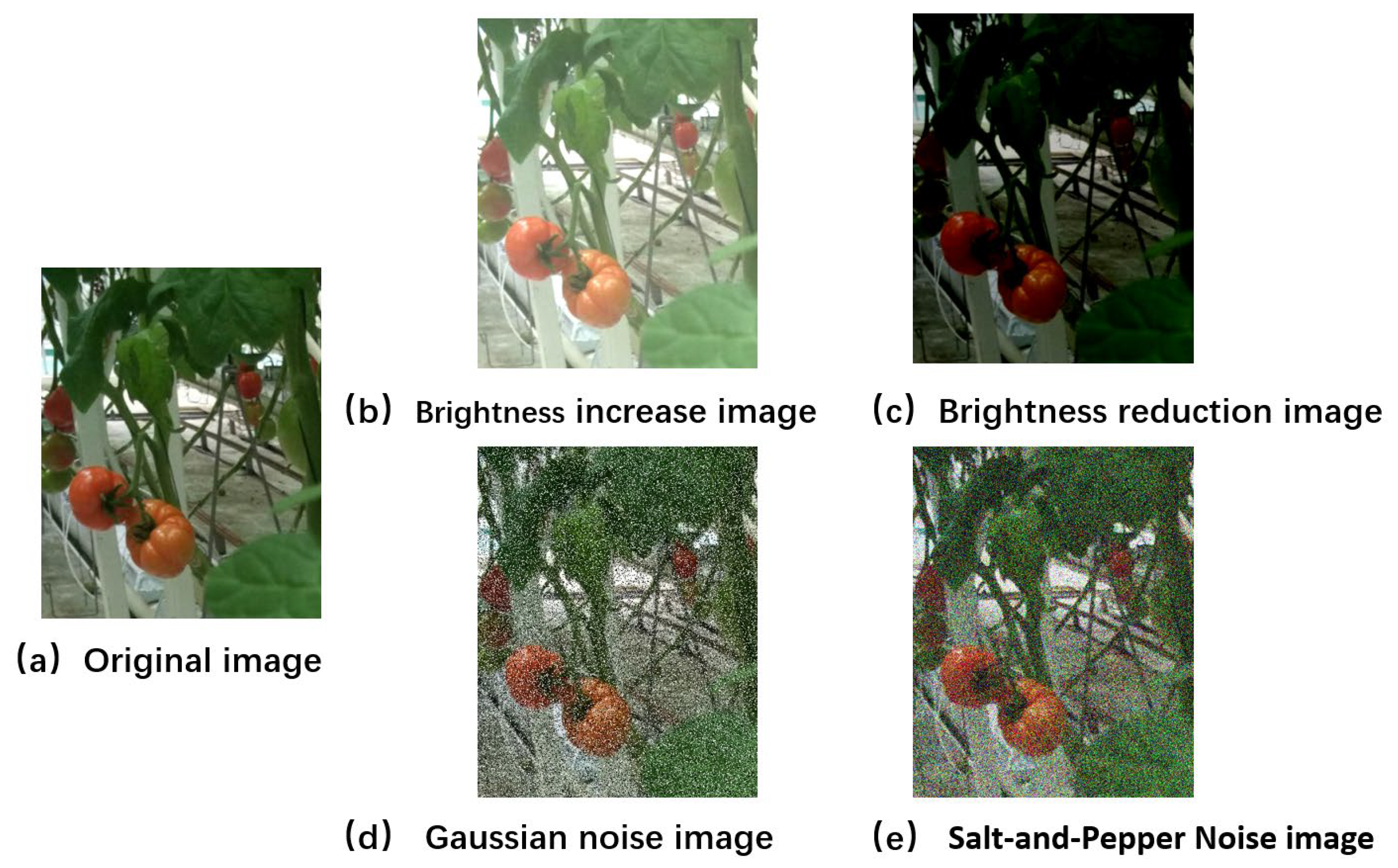
To enhance the model’s robustness against environmental variations inherent in greenhouse scenarios (e.g., uneven lighting, sensor noise, and chromatic distortions), we implemented a comprehensive data augmentation pipeline. These augmentation methods and parameter settings were adopted based on the approach proposed by Lin et al. (2025) [49], which demonstrated strong performance in tomato detection tasks. Specifically, three augmentation strategies were applied stochastically during training, with a probability of 0.5.

• Brightness Variation: Randomly adjust the luminance channel in HSV color space within a ±20% range to simulate illumination fluctuations caused by greenhouse shading systems and diurnal light changes.
• Additive Gaussian Noise: Inject zero-mean Gaussian noise with a standard deviation of σ = 25 into the RGB channels. This operation simulates sensor noise deriving from low-cost agricultural imaging devices and environmental illumination instability. The noise is spatially variant, with random regions selected for perturbation to avoid uniform degradation.
• Salt-and-Pepper Noise: Randomly corrupt 10% of pixels with binary impulse noise (0 or 255 values) at a probability of 0.1. This mimics transient occlusions from dust particles, water droplets on camera lenses, and sensor circuit anomalies.

These augmentations were executed in parallel with standard techniques (random horizontal flipping, scaling [0.5×, 2.0×], and 512 × 512 center cropping) to ensure multi-view consistency. The Gaussian noise parameterization (μ = 0, σ = 25) ensured realistic signal-to-noise ratio degradation, while the salt-and-pepper noise introduced structured artifacts that challenge boundary localization. The pipeline reduces the risk of overfitting by expanding the effective training samples eightfold while preserving critical morphological features (e.g., fruit–stem junctions). As shown in Figure 3, a data set of 4475 images was finally obtained, which is divided into training, validation, and test sets according to the ratio of 7:2:1. Therefore, 3200, 895, and 380 images were used for training, validation, and testing of the model, respectively.

2.3. Enhanced Multi-Scale Feature Extraction via SAConv and WTConv

The detection of tomatoes in greenhouse environments is significantly hindered by severe occlusions caused by overlapping leaves, stems, and densely clustered fruits, frequently resulting in partial or complete invisibility of targets and the consequent degradation of detection accuracy. The intricate foliage density and dynamic growth patterns inherent to tomato plants create hierarchical occlusion scenarios characterized by transient visibility through leaf gaps or persistent obscuration under multi-layered foliage coverage. While the traditional YOLO11 architecture demonstrates efficacy in general object detection tasks, it exhibits three critical limitations under such conditions: First, the fixed receptive field mismatch stems from standard convolutions employing static kernel sizes, leading to a lack of adaptability to spatially varying occlusion geometries. This limitation manifests prominently when detecting tomatoes obscured by intersecting stems, where single-scale convolutions fail to reconcile the simultaneous extraction of fine local textures (e.g., surface gloss in exposed regions) and long-range contextual cues (including stem connections beyond occluded areas). Second, high-frequency feature degradation arises from the conventional stride-2 down-sampling operations in the YOLOv11 backbone, which irreversibly suppress critical high-frequency components that are essential for identifying the sub-pixel edge details and texture patterns of small tomatoes. Third, performing homogeneous feature extraction Via uniform spatial convolution neglects the spatially heterogeneous significance of features, notably failing to prioritize structurally critical regions such as stem junctions near occlusions while inadequately suppressing uniform background foliage. To address these limitations, we propose a dual-branch enhancement module integrating SAConv and WTConv. The synergy between SAConv and WTConv enables occlusion-adaptive multi-scale perception: SAConv resolves the “see-through” problem in dense foliage by dynamically associating local and global cues, while WTConv ensures pixel-level fidelity for sub-visible targets. This dual mechanism effectively bridges the gap between robustness to occlusion and detail preservation, forming the cornerstone of our detection framework.

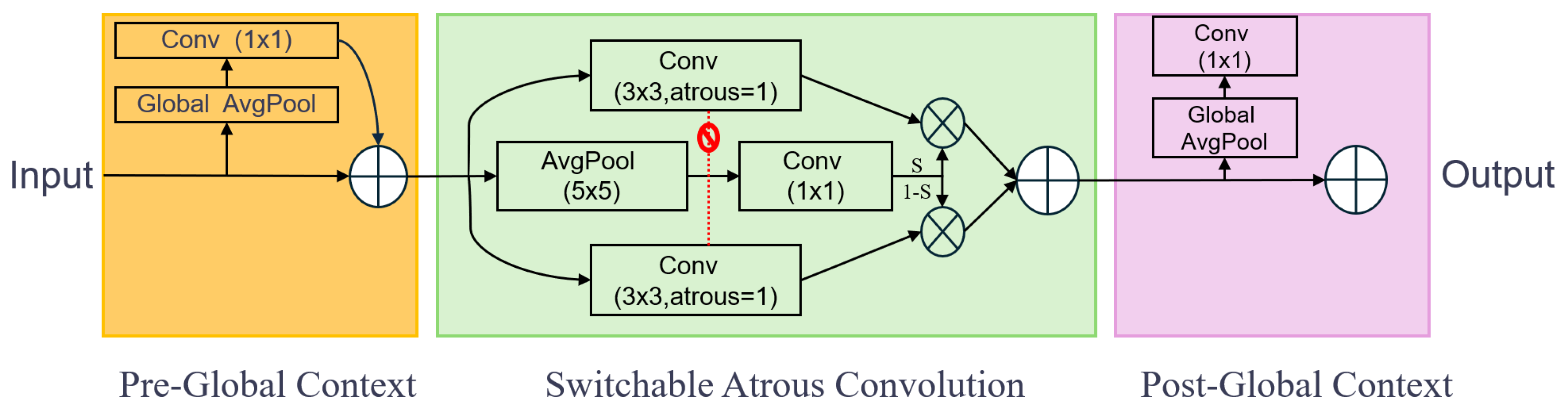
To strengthen the backbone’s multi-scale receptive field, this work integrates the SAConv module. Originally proposed by Qiao et al. in 2021 [50], SAConv applies convolutions with multiple atrous rates on the same feature map and adaptively merges their outputs Via spatially dependent switch functions. As shown in Figure 4, the SAConv model is divided into three parts, as follows: The first part is pre-global context, where the feature map undergoes a 1 × 1 convolution and global average pooling for inter-channel information compression and enhancement to extract the global context information. The second part is switchable atrous convolution with two parallel branches. The null convolution branch involves a 3 × 3 convolution with different null rates being used for processing, where one branch has a null rate of 1 and the other has a null rate of 3, thus helping to expand the convolution’s sensory field without increasing the computational cost and capture richer multi-scale information. On the other hand, the average pooling branch involves a 5 × 5 average pooling operation being performed to further capture local information. Finally, the results of the two branches are integrated Via a 1 × 1 convolution. The third part is the post-global context, which integrates the global information again after 1 × 1 convolution and global average pooling. For the switchable mechanism, a dynamic weighting parameter S allows for switching between the null convolution and average pooling results. According to the different needs of the task, the module can adaptively adjust the attention to local details and global features. The specific convolution formula is shown in Equation (1):

$$y=\mathbf{C}\mathbf{o}\mathbf{n}\mathbf{v}\left(\mathbf{x},\mathbf{w},1\right)\stackrel{\mathbf{C}\mathbf{o}\mathbf{n}\mathbf{v}\mathbf{e}\mathbf{r}\mathbf{t}}{\to }\mathbf{S}\left(\mathbf{x}\right)\cdot \mathbf{C}\mathbf{o}\mathbf{n}\mathbf{v}\left(\mathbf{x},\mathbf{w},1\right)+\left(1-\mathbf{S}\left(\mathbf{x}\right)\right)\cdot \mathbf{C}\mathbf{o}\mathbf{n}\mathbf{v}\left(\mathbf{x},\mathbf{w}+\Delta \mathbf{w},r\right),$$

(1)

where y denotes the output of the convolution operation, x represents the feature map input to the convolution operation, w is the weight matrix (convolution kernel) used for the convolution operation, Convert denotes convert a convolutional layer to SAC. Δw is the offset of the convolution kernel, r is the nulling rate of the null convolution, and S(x) is a function that computes a value, based on the input feature map x, which is used to control whether or not the standard convolution kernel w or the modified convolution kernel Δw is used.

To enhance the receptive field and incorporate frequency domain information, the WTConv (wavelet convolution) module is further integrated into the backbone. This module was originally proposed by Finder et al. in 2024 [51], and its core idea is to combine wavelet decomposition with convolutional operations. Leveraging multi-scale frequency representations, WTConv enables the network to capture both local and global features more effectively. Compared to standard convolutions, WTConv improves the model’s ability to perceive structured patterns, which is especially beneficial for detecting tomatoes under complex greenhouse backgrounds. As shown in Figure 5, with WTConv, the model performs a multi-level decomposition of the input image using a two-dimensional Haar wavelet transform. The Haar wavelet transform uses four filters to decompose the image into four sub-bands: the low-frequency component (LL), horizontal high-frequency component (LH), vertical high-frequency component (HL), and diagonal high-frequency component (HH), which are used to capture low-frequency information in the image, such as the overall shape or contours; horizontal edge information in the image; vertical edge information in an image; and the diagonal details of the image, respectively. The convolution method is shown in Equation (2):

$$f_{LL}={\displaystyle \frac{1}{2}}\left[\begin{array}{cc}1& 1\\ 1& 1\end{array}\right],f_{LH}={\displaystyle \frac{1}{2}}\left[\begin{array}{cc}1& -1\\ 1& -1\end{array}\right],f_{HL}={\displaystyle \frac{1}{2}}\left[\begin{array}{cc}1& 1\\ -1& -1\end{array}\right],f_{HH}={\displaystyle \frac{1}{2}}\left[\begin{array}{cc}1& -1\\ -1& 1\end{array}\right].$$

(2)

Equation (3) shows the output of the convolution:

$$\left[X_{LL},X_{LH},X_{HL},X_{HH}\right]=\mathrm{C}\mathrm{o}\mathrm{n}\mathrm{v}\left(\left[f_{LL},f_{LH},f_{HL},f_{HH}\right],X\right),$$

(3)

where X_LL is the low-frequency component of X; and X_LH, X_HL, and X_HH are the horizontal, vertical, and diagonal high-frequency components of X, respectively.

At each level of the wavelet transform, the image is down-sampled (i.e., its spatial resolution is halved), while the frequency information is decomposed to a finer level. The inverse wavelet transform (IWT) is then obtained using transposed convolution, as shown in Equation (4):

$$X=\mathrm{Conv}-\mathrm{transposed}\left(\left[f_{LL},f_{LH},f_{HL},f_{HH}\right],\left[{\mathrm{X}}_{LL},{\mathrm{X}}_{LH},{\mathrm{X}}_{HL},{\mathrm{X}}_{HH}\right]\right).$$

(4)

After completing the convolution, the cascaded wavelet decomposition is obtained by recursively decomposing the low-frequency components. Finally, the convolution results for each sub-band are re-synthesized into a complete output using the IWT. Equations (5) and (6) show the computation of the inverse wavelet transform:

$$X_{LL}^{\left(i\right)},X_{LH}^{\left(i\right)},X_{HL}^{\left(i\right)},X_{HH}^{\left(i\right)}=\mathrm{W}\mathrm{T}\left(X_{LL}^{\left(i-1\right)}\right)$$

(5)

$$Y=\mathrm{I}\mathrm{W}\mathrm{T}\left(\mathrm{C}\mathrm{o}\mathrm{n}\mathrm{v}\left(W,\mathrm{W}\mathrm{T}\left(X\right)\right)\right)$$

(6)

where X_LL⁽⁰⁾ = X, i denotes the current level, and X and W are the input tensor and weight tensor of a k × K deep convolutional kernel with four times as many input channels, respectively.

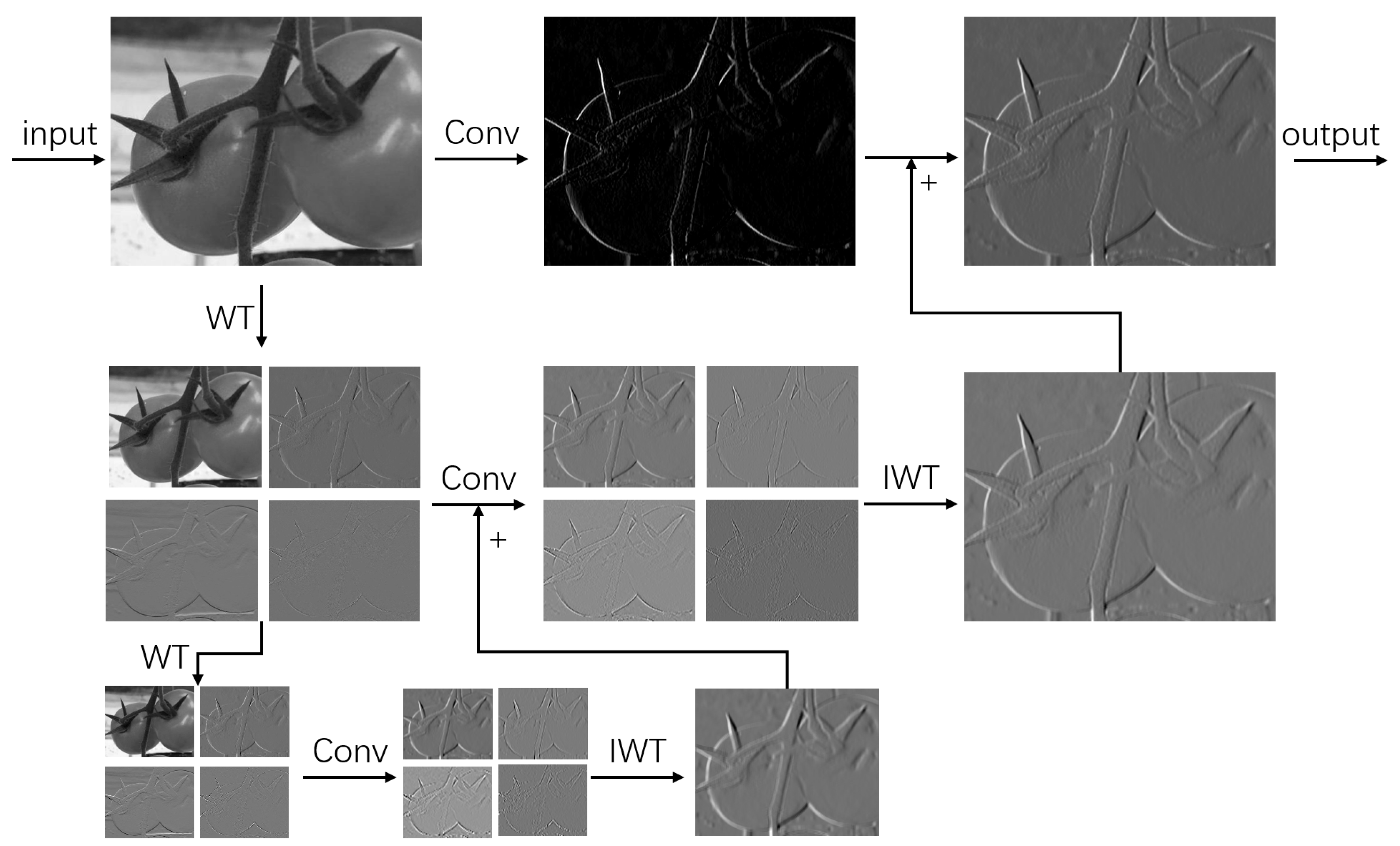
To better illustrate how WTConv enhances feature extraction across different frequency bands, we provide a detailed visualization in Figure 6. The figure shows the intermediate results of applying two-level Haar wavelet decomposition to a greenhouse tomato image, followed by convolution operations on each sub-band and the final reconstruction Via inverse wavelet transforms. This multi-scale, frequency-aware structure allows the model to capture both fine-grained edges (from high-frequency bands) and global shape information (from low-frequency bands), which is especially beneficial for detecting tomatoes of varying size and appearance in complex greenhouse environments.

2.4. Adaptive DySample Module in the Neck Layer

The detection system encounters substantial challenges due to dynamic and heterogeneous illumination conditions in the context of tomato detection in greenhouses, as natural sunlight penetrating through greenhouse covers and artificial LED lighting induce spatially varying photometric distortions. Localized over-exposure on tomato surfaces results in pixel saturation and the loss of critical texture details, while intermittent shadows from foliage structures reduce contrast ratios, thus blurring target boundaries. Moreover, abrupt illumination transitions, such as cloud movements or light fixture flickering, introduce high-frequency noise artifacts that exacerbate the information loss that occurs during conventional down-sampling. Collectively, these factors degrade the feature representation of tomato images. The conventional YOLO11 architecture employs uniform sampling operations to indiscriminately suppress both noise and high-frequency discriminative features—a strategy that lacks adaptability to spatially varying light patterns.

To address these challenges, the up-sampling operator DySample is integrated into the SWMD-YOLO architecture for illumination-aware feature reconstruction. DySample is a lightweight and efficient up-sampling method based on dynamic point sampling. Its core mechanism involves dynamically adjusting sampling positions by generating content-aware offsets instead of relying on the computationally intensive operations of traditional dynamic convolution kernels. This method first optimizes the initial sampling locations using bilinear initialization, thus ensuring a uniform distribution of sampling points. It then controls the range of offsets with static and dynamic range factors, thereby mitigating sensitivity to color distortion and preserving frequency-specific details, such as faint surface wrinkles on unripe tomatoes or glossy variations in occluded fruits. Additionally, features are grouped to independently generate offsets, reducing redundancy and ensuring robust feature fusion under varying lighting scenes without compromising computational efficiency. This approach enhances both the efficiency and performance of the model. Figure 7 illustrates the DySample module framework.

DySample revisits the core mechanism of up-sampling through dynamic sampling-based up-sampling, focusing on discrete coordinate selection operations. This framework establishes that adaptive sampling positions can be effectively determined through parametric learning, rather than predefined interpolation rules. As demonstrated in Figure 7, the grid sampling operation processes an input feature tensor X with dimensions [C, H₁, W₁] using a two-dimensional coordinate tensor S of size [2, H₂, W₂], where the first channel contains normalized horizontal coordinates and the second contains vertical coordinates. This mechanism allows for coordinate-guided bilinear interpolation through mapping each position in the target grid S to corresponding sub-pixel locations in the source feature map X. Through differentiable warping operations, the original feature representation is spatially transformed into an output tensor X’ of dimensions [C, H₂, W₂], effectively establishing continuous feature correspondence between input and output resolutions. This process is defined as

$${\mathcal{X}}^{\prime }=grid\_sample\left(\mathcal{X},\mathcal{S}\right)$$

(7)

Given an up-sampling scale factor s and an input feature map X ∈ R^[C,H,W], a linear transformation layer (input/output channels: C→2s²) generates an offset tensor O ∈ R ^[2,sH,sW]. This tensor is spatially restructured to dimensions R ^[2,sH,sW] using the pixel shuffling algorithm [52], producing a rescaled offset $\mathcal{O}$. Finally, the sampling set $\mathcal{S}$ is obtained through superposition of the offset $\mathcal{O}$ and the original sampling grid $\mathcal{G}$. This process is defined as

$$\mathcal{O}=\mathrm{l}\mathrm{i}\mathrm{n}\mathrm{e}\mathrm{a}\mathrm{r}\left(\mathcal{X}\right),$$

(8)

$$\mathcal{S}=\mathcal{G}+\mathcal{O}.$$

(9)

The description of the reshaping operation is omitted here. Finally, the up-sampled feature map ${\mathcal{X}}^{\prime }$, with dimensions [C, sH, sW], is generated Via the sampling set and the grid_sample function, as in Equation (7).

2.5. Multi-Scale Convolutional Attention Module in Neck Layer

In the intelligent greenhouse tomato detection task, the target detection model needs to cope with the dual challenges of significant target scale differences and frequent branch and leaf occlusion, which imposes severe requirements on the model’s perceptual ability and computational efficiency.

In terms of the target scale difference, the pixel span between the near-view ripe fruits and the far-view young fruits (with pixel sizes larger than 128 × 128 and pixel sizes smaller than 32 × 32, respectively) can be up to 5–10 times. For near-view fruits, fine-grained features such as surface textures like color gradient, glossiness, and near-circular geometries need to be captured, while the localization of far-view young fruits is reliant on global contextual information due to their blurred outlines and similar colors to the leaves. In traditional methods, the most commonly used 3 × 3 or 5 × 5 kernel single-scale convolution leads to difficulties in balancing local details and the global distribution due to the fixed receptive field. Although the neck layer of YOLO11 integrates FPN and PAN structures to enhance the detection of targets through multi-scale feature fusion, which alleviates part of the problem, high-level semantic features can still obscure the low-level fine-grained information such as the fruit–stalk connection structure. The branch and leaf occlusion problem is particularly prominent in dense planting environments, where about 30% of the fruits are partially or completely occluded by leaves and artificial facility infrastructure (e.g., greenhouse support frames and drip irrigation tubes) may be similar in morphology to the fruits, exacerbating feature confusion. Conventional convolutional kernels are prone to producing “blind responses” in the occluded region, such as false positive detection when the leaves are similar in color to the young fruits, whereas the asymmetric response peaks at the occluded boundaries interfere with the accuracy of bounding box regression. In addition, although Transformer-based self-attention mechanisms can help to model global relationships, their computational complexity (O(n²)) leads to insufficient real-time performance in 1024 × 1024 high-resolution images, resulting in an inference frame rate of <40 FPS for the edge devices commonly used in such environments and the assignment of redundant weights to invalid occluded regions.

The unique requirements of agricultural detection scenarios further increase the complexity of model design. In terms of morphological adaptation, as the stalks of tomato fruit are elongated, the model is required to capture long-distance spatial dependence in the connection relationship between fruit stalks and main branches; meanwhile, in terms of fruit color dynamics, tomato fruits change dynamically from green to red, which requires channel attention to dynamically enhance the response to key color channels.

To address the above challenges, this study introduces the MSCA module, which collaboratively captures spatial context at different scales through multi-branch depth-separable strip convolution (7 × 1 + 1 × 7, 11 × 1 + 1 × 11, 21 × 1 + 1 × 21); in particular, a large kernel convolution (21 × 21) and a small–medium kernel convolution model the global distribution of the plant to localize the distant-view young fruits and extract the local details of near-view fruits with residual connectivity, respectively, retaining local details and the gradient information of fine-grained structures such as fruit stalks through residual concatenation. At the same time, the occlusion mask generated Via deformable convolution and the dynamic spatial attention mechanism are combined to suppress the ineffective response in the leaf region. The lightweight design (depth-separable convolution reduces the number of parameters by 90%) and linear computational complexity of MSCA provide an efficient solution to the needs of multi-scale target detection and occlusion resistance in complex agricultural scenarios.

The MSCA module captures spatial features at different scales through multi-branch depth-separable strip convolution with cascade operations of 7 × 1 with 1 × 7, 11 × 1 with 1 × 11, and 21 × 1 with 1 × 21. The 21 × 21 large kernel convolution is used to capture global contextual information in order to localize the contour features of the far-field target, and the 7 × 7 and 11 × 11 small and medium kernel convolutions, respectively, are used to extract local details such as textures and edges. These multi-scale features are fused with the original localized features through residual concatenation, preserving the critical fine-grained information of the fruit stalk connection structure. Subsequently, the aggregated features are channel-blended through 1 × 1 convolution to generate a spatial attention weight matrix, as shown in Equation (10), and the input features are dynamically calibrated Via element-wise multiplication, as shown in Equation (11), where F denotes the input features and Att and Out are the attention input and output, respectively. ⊗, DW–Conv, and i ∈ {0,1,2,3} denote the element-wise matrix multiplication operation, the depth convolution and scale, and the branch index, respectively. A Scale₀ denotes a constant connection using two depth-direction strip convolutions to approximate the standard depth-direction convolution with large kernels, and the kernel size of each branch is set to 7, 11, and 21. This design not only solves the problem regarding the insufficient sensory field of the traditional single-scale convolution, but also suppresses the ineffective response of the leaf-covered region through the attention mechanism. Figure 8 illustrates the framework of the proposed MSCA module.

$$\mathrm{A}\mathrm{t}\mathrm{t}={\mathrm{C}\mathrm{o}\mathrm{n}\mathrm{v}}_{1\times 1}\left(\sum _{i=0}^3{\mathrm{S}\mathrm{c}\mathrm{a}\mathrm{l}\mathrm{e}}_i\left(\mathrm{D}\mathrm{W}-\mathrm{C}\mathrm{o}\mathrm{n}\mathrm{v}\left(F\right)\right)\right),$$

(10)

$$\mathrm{O}\mathrm{u}\mathrm{t}=\mathrm{A}\mathrm{t}\mathrm{t}\otimes F.$$

(11)

2.6. Improved Loss Function

In the greenhouse tomato detection task, the targets often present a small size (e.g., the pixel dimensions of young fruits in the distant view are generally <32 × 32) and irregular morphology (e.g., leaf occlusion leads to significant differences in the aspect ratio of the bounding box) in dense planting scenes. Traditional bounding box regression loss functions (e.g., IoU, GIoU, SIoU) mainly focus on the geometric position of the prediction box and the real box, but ignore the dual impact of the target’s morphological features on the regression accuracy. On one hand, the scale span of mature and young fruits can be up to 5–10 times greater, and it is difficult for existing loss functions to balance the optimization weights of the targets at different scales; on the other hand, the effective detection area of fruits may be asymmetrically distributed as a result of foliage occlusion. Leaf shading also results in an asymmetric distribution of the effective detection area of the fruit (e.g., the fruit is only locally visible), and the traditional loss functions are unable to effectively capture this kind of shape aberration. Although YOLOv11 is an advanced detection framework, its bounding box regression module still adopts the traditional loss calculation paradigm, which makes it difficult for the model to accurately quantify the boundary alignment when there is a significant difference in the aspect ratio between the real and predicted frames (e.g., if the shank junction has an abnormal aspect ratio of the predicted frame due to occlusion). In addition, the existing methods fail to fully explore the morphological information (e.g., principal axis direction, local curvature) and scale features (e.g., if the real projected area) of the bounding box, which can lead to limited model convergence speed and an elevated misdetection rate in complex occlusion scenarios. For example, when ripe fruits (sub-circular, area > 128 × 128 pixels) and young fruits (ellipsoidal, area < 32 × 32 pixels) coexist, the homogenization optimization strategy of the traditional loss function causes the small object regression gradient to be dominated by that of the large object, resulting in an increased misdetection rate of the young fruits in the distant view.

In our study, we introduce Focaler-IoU—a novel loss function designed to address the imbalance between difficult (low IoU) and easy (high IoU) samples in bounding box regression. This method is integrated as a new regression loss function into our SWMD-YOLO framework in order to enhance the detection accuracy of tomatoes in greenhouse environments; particularly for small or occluded targets.

Focaler-IoU builds upon existing IoU-based loss functions. We first define these foundational metrics.

• IoU (Intersection over Union)

The baseline metric for evaluating the overlap between predicted box $B$ and the ground truth box $B^{gt}$:

$$IoU={\displaystyle \frac{|B\cap B^{gt}|}{|B\cup B^{gt}|}}.$$

(12)

2.

GIoU (Generalized IoU)

This addresses gradient vanishing when $B$ and $B^{gt}$ do not overlap:

$$GIoU=IoU-{\displaystyle \frac{|C-B\cap B^{gt}|}{\left|C\right|}}$$

(13)

where $C$ is the smallest enclosing box of $B$ and $B^{gt}$.

3.

DIoU (Distance-IoU)

This adds a normalized centroid distance penalty:

$$DIoU=IoU-{\displaystyle \frac{{\rho }^2\left(b,b^{gt}\right)}{c^2}},$$

(14)

where $\rho$ is the Euclidean distance between centroids $b$ and $b^{gt}$, and $c$ is the diagonal length of $C$.

4.

CIoU (Complete IoU)

This extends DIoU with aspect ratio constraints:

$$CIoU=IoU-{\displaystyle \frac{{\rho }^2\left(b,b^{gt}\right)}{c^2}}-\alpha v,$$

(15)

$$\alpha ={\displaystyle \frac{v}{(1-IoU)+v}},$$

(16)

$$v={\displaystyle \frac{4}{{\pi }^2}}(arctan{\displaystyle \frac{w^{gt}}{h^{gt}}}-arctan{\displaystyle \frac{w}{h}}{)}^2,$$

(17)

where $w^{gt}$ and $h^{gt}$ are the width and height of the GT box, respectively; and $w$ and $h$ are the width and height of the anchor box, respectively.

5.

EIoU (Efficient IoU)

This directly minimizes width/height discrepancies:

$$EIoU=IoU-{\displaystyle \frac{{\rho }^2\left(b,b^{gt}\right)}{c^2}}-{\displaystyle \frac{{\rho }^2\left(w,w^{gt}\right)}{(w^c{)}^2}}-{\displaystyle \frac{{\rho }^2\left(h,h^{gt}\right)}{(h^c{)}^2}},$$

(18)

where $w^c$ and $h^c$ denote the width and height of $C$, respectively.

6.

SIoU (Scylla IoU)

This incorporates angle alignment for faster convergence:

$$SIoU=IoU-{\displaystyle \frac{\left(\Delta +\Omega \right)}{2}},$$

(19)

$$\Lambda =sin\left(2si{n}^{-1}{\displaystyle \frac{\min \left(\left|x_c^{gt}-x_c\right|,\left|y_c^{gt}-y_c\right|\right)}{\sqrt{(x_c^{gt}-x_c{)}^2+(y_c^{gt}-y_c{)}^2}+\in }}\right),$$

(20)

$$\Delta =\sum _{t=w,h}\left(1-e^{-\gamma {\rho }_t}\right),\gamma =2-\Lambda ,$$

(21)

$$\left\{\begin{array}{c}{\rho }_x=\hspace{0.25em}\hspace{0.25em}\hspace{0.25em}\hspace{0.25em}({\displaystyle \frac{x_c-x_c^{gt}}{w^c}}{)}^2\hfill \\ {\rho }_y=\hspace{0.25em}\hspace{0.25em}\hspace{0.25em}\hspace{0.25em}({\displaystyle \frac{y_c-y_c^{gt}}{h^c}}{)}^2\hspace{0.25em}\hspace{0.25em}\hspace{0.25em}\hspace{0.25em}\hfill \end{array}\right.,$$

(22)

$$\Omega =\sum _{t=w,h}(1-e^{-{\omega }_t}{)}^{\theta },\theta =4,$$

(23)

$$\left\{\begin{array}{c}{\omega }_w=\hspace{0.25em}\hspace{0.25em}\hspace{0.25em}\hspace{0.25em}{\displaystyle \frac{|w-w_{gt}|}{max(w,w_{gt})}}\hfill \\ {\omega }_h=\hspace{0.25em}\hspace{0.25em}\hspace{0.25em}\hspace{0.25em}{\displaystyle \frac{|h-h_{gt}|}{max(h,h_{gt})}}\hspace{0.25em}\hspace{0.25em}\hspace{0.25em}\hspace{0.25em}\hfill \end{array}\right..$$

(24)

To address the issue of sample imbalance, we propose Focaler-IoU, which dynamically adjusts the attention paid to difficult and easy samples Via linear interval mapping. The reconstructed IoU value $Io{U}^{focaler}$ is defined as follows:

$$Io{U}^{focaler}=\left\{\begin{array}{c}0,\hspace{0.25em}\hspace{0.25em}\hspace{0.25em}\hspace{0.25em}\hspace{0.25em}\hspace{0.25em}\hspace{0.25em}\hspace{0.25em}\hspace{0.25em}\hspace{0.25em}\hspace{0.25em}\hspace{0.25em}IoU<d\hfill \\ {\displaystyle \frac{IoU-d}{u-d}},\hspace{0.25em}\hspace{0.25em}\hspace{0.25em}\hspace{0.25em}d\ll IoU\ll u\hfill \\ 1,\hspace{0.25em}\hspace{0.25em}\hspace{0.25em}\hspace{0.25em}\hspace{0.25em}\hspace{0.25em}\hspace{0.25em}\hspace{0.25em}\hspace{0.25em}\hspace{0.25em}\hspace{0.25em}\hspace{0.25em}IoU>u\hspace{0.25em}\hspace{0.25em}\hspace{0.25em}\hspace{0.25em}\hfill \end{array}\right.,$$

(25)

where [d,u] ∈ [0,1] are tunable thresholds. For greenhouse tomato detection, we set d = 0.3 and u = 0.7 to prioritize medium-difficulty samples (e.g., partially occluded tomatoes).

The final loss is derived as follows:

$$L_{\mathrm{Focaler}-\mathrm{IoU}}=1-Io{U}^{focaler}.$$

(26)

Focaler-IoU can seamlessly be combined with GIoU, DIoU, CIoU, EIoU, and SIoU as follows:

$$L_{Focaler-GIoU}=L_{GIoU}+IoU-Io{U}^{Focaler},$$

(27)

$$L_{Focaler-GIoU}=L_{GIoU}+IoU-Io{U}^{Focaler},$$

(28)

$$L_{Focaler-GIoU}=L_{GIoU}+IoU-Io{U}^{Focaler},$$

(29)

$$L_{Focaler-EIoU}=L_{EIoU}+IoU-Io{U}^{Focaler},$$

(30)

$$L_{Focaler-SIoU}=L_{SIoU}+IoU-Io{U}^{Focaler}.$$

(31)

In SWMD-YOLO, we adopt $L_{Focaler-SIoU}$ (Equation (31)) as the default loss function, leveraging SIoU’s angle alignment for the precise localization of clustered tomatoes. The linear mapping thresholds (d = 0.3, u = 0.7) were optimized for greenhouse scenarios, where small and overlapping tomatoes dominate. This configuration enhances gradients for medium-difficulty samples while suppressing outliers (IoU < 0.3) and overconfident predictions (IoU > 0.7).

2.7. Experimental Environment and Parameter Setting

The experiments were implemented using the PyTorch deep learning framework. The training hyperparameters used in this study were selected with reference to the settings proposed by Sun et al. (2024) [47], and the detailed hyperparameter settings are outlined in

Table 1. Experimental environment configuration.

Environment	Version	Hyperparameter	Setting
OS	Windows 11 x64	Input Resolution	640 × 640
CPU	i7-12700KF	Initial Learning Rate	0.01
GPU	RTX 4070 Ti SUPER	Learning Rate Float	0.01
CUDA	12.1	Batch Size	16
PyTorch	2.4.1	Workers	8
Python	3.9	Epochs	300

. The GB RAM for the RTX 4070 Ti SUPER is 16 GB. To optimize the training dynamics, we adopted a cosine annealing scheduler to adjust the learning rates and network weights over 300 training epochs, ensuring smooth transitions between the exploration and exploitation phases. Stochastic Gradient Descent (SGD) was selected as the optimizer due to its computational efficiency and compatibility with large-scale models, configured with a momentum factor of 0.937 to stabilize gradient updates and accelerate convergence, coupled with a weight decay of 5 × 10⁻⁴ to regularize model complexity and mitigate the risk of overfitting. The initial learning rate was set to 0.01 in order to rapidly reduce loss during early training while avoiding instability due to excessive gradient steps.

2.8. Evaluation Metrics

The evaluation metrics used for the object detection task mainly reflected the model complexity, number of parameters, and computational load. To fully evaluate the greenhouse tomato detection model, five metrics were used: Precision, recall, average precision(AP), mAP50-95, and FPS. Specifically, map50-95 denotes the average mean precision at the Intersection over Union (IoU) threshold of 0.5 to 0.95. The formulas for calculating these metrics are as follows:

$$Precision={\displaystyle \frac{TP}{TP+FN}}\times 100\mathrm{\%},$$

(32)

$$Recall={\displaystyle \frac{TP}{TP+FP}}\times 100\mathrm{\%},$$

(33)

$$\mathrm{A}\mathrm{P}={\int }_0^1\mathrm{P}\left(R\right)\mathrm{d}\mathrm{R},$$

(34)

$$\mathrm{m}\mathrm{A}\mathrm{P}50-95={\displaystyle \frac{1}{10}}\sum _{i=1}^{10}{\mathrm{A}\mathrm{P}}_{IoU=0.5+i\cdot 0.05},$$

(35)

$$\mathrm{F}\mathrm{P}\mathrm{S}=1/T,$$

(36)

where TP, FP, and FN denote the number of images in which the model correctly detects tomato fruit targets, the number of images in which the model incorrectly detects non-tomato fruit targets, and the number of images in which the model fails to detect tomato fruit targets, respectively. Precision and recall denote the accuracy rate and recall rate, respectively. These rates are used to construct the accuracy–recall curve (PR curve), the area under which is defined as the average detection rate AP. mAP50-95 denotes the average AP for IoU thresholds ranging from 0.5 to 0.95. T and FPS denote the detection time for a single image and the number of images detected per second, respectively.

In this study, the evaluation metrics include precision, recall, mAP50, and mAP95—are computed based on the correct localization of all visible tomato fruits, regardless of maturity level. That is, both fully ripe (red) and unripe (green or yellowish) tomatoes are treated as valid detection targets, provided they are labeled in the data set. No ripeness classification is involved in this task. The ground-truth annotations were manually verified, and ambiguous samples were excluded to ensure consistency in the evaluation process. The primary objective of this work is to detect the presence and location of tomato fruits in complex greenhouse environments, rather than to classify their maturity stages.

3. Experiments and Results

3.1. Evaluation of Model Performance and Size

To validate the effectiveness of SWMD-YOLO, the improved YOLO model was compared with the baseline model using the same training data set. As shown in

Table 2. Comparison of YOLOv11n and SWMD-YOLO on the tomato data set.

Methods	Precision (%)	Recall (%)	mAP50 (%)	mAP95 (%)	FPS	Parameters (M)	Model Size (MB)	GFLOPs
YOLOv11n	90.35	82.85	90.02	61.26	70.21	4.28	6.8	6.9
SWMD-YOLO	92.78	86.09	93.47	65.74	75.68	3.47	6.4	5.7

, SWMD-YOLO outperformed the baseline model across all performance metrics, including mean average precision (mAP50 and mAP95), recall, and FPS, with improvements of 3.83%, 4.48%, 6.18%, and 3.24%, respectively. The observed improvements can mainly be attributed to the convolutional module with enhanced multi-scale feature extraction capability. This module combines SAConv and WTConv to capture multi-scale feature information by dynamically adjusting the atrous ratio and wavelet decomposition, significantly improving the ability to detect occluded tomatoes and small objects. In addition, the dynamic up-sampling mechanism (DySample) in the neck layer replaces the traditional down-sampling, which adaptively adjusts the up-sampling strategy, reduces feature loss, effectively restores detail information, and improves detection accuracy under complex backgrounds. Finally, the key regions are strengthened using the attention mechanism; in particular, MSCA is introduced to integrate local and global information through multi-branch deep convolution, dynamically allocate attention weights, suppress background noise interference, and enhance the representation of key features.

Compared to the original YOLOv11n baseline, SWMD-YOLO achieves a compact model size of 6.4 MB and a parameter count of 3.47 M, comprising reductions of 5.9% and 18.9%, respectively. These improvements are mainly due to the introduction of the SAConv module, which utilizes the extended convolution as its core building block and greatly reduces the parameter count of the model.

To further evaluate the models’ performance, PR curves were generated during testing at an IOU threshold of 0.5, comparing the results before and after the improvement, as shown in Figure 9. The precision–recall curve is an important tool for evaluating the performance of a target detection model, with recall on the horizontal axis and precision on the vertical axis. By plotting the relationship between precision and recall under different classification thresholds, the PR plot intuitively reflects the trade-off ability of the model for target detection under different confidence levels.

The PR curve of YOLO11n reveals high precision at low recall (recall < 40%); however, the precision decreases significantly as the recall increases (e.g., detecting more occlusions or small targets). This suggests that the baseline model is not sufficiently adaptable to complex scenes, and the false detection rate (FP) is elevated at high recall. This is due to the fact that YOLO11n lacks a multi-scale feature optimization module and has a weak feature fusion capability for small targets and occluded scenes. The PR curve of SWMD-YOLO is overall closer to the upper right, especially at recall rates > 40%, indicating that it still maintains a high precision rate. This shows that the model can simultaneously balance a high recall and low false detection rate in complex scenes. This is achieved through enhanced multi-scale feature extraction with SAConv and WTConv, optimized detail recovery with DySample, and suppressed background interference with MSCA. Figure 9 shows that the mAP50 of YOLO11n is 90.02%, while that of SWMD-YOLO improves to 93.47%, verifying the significant difference in the area under the curve.

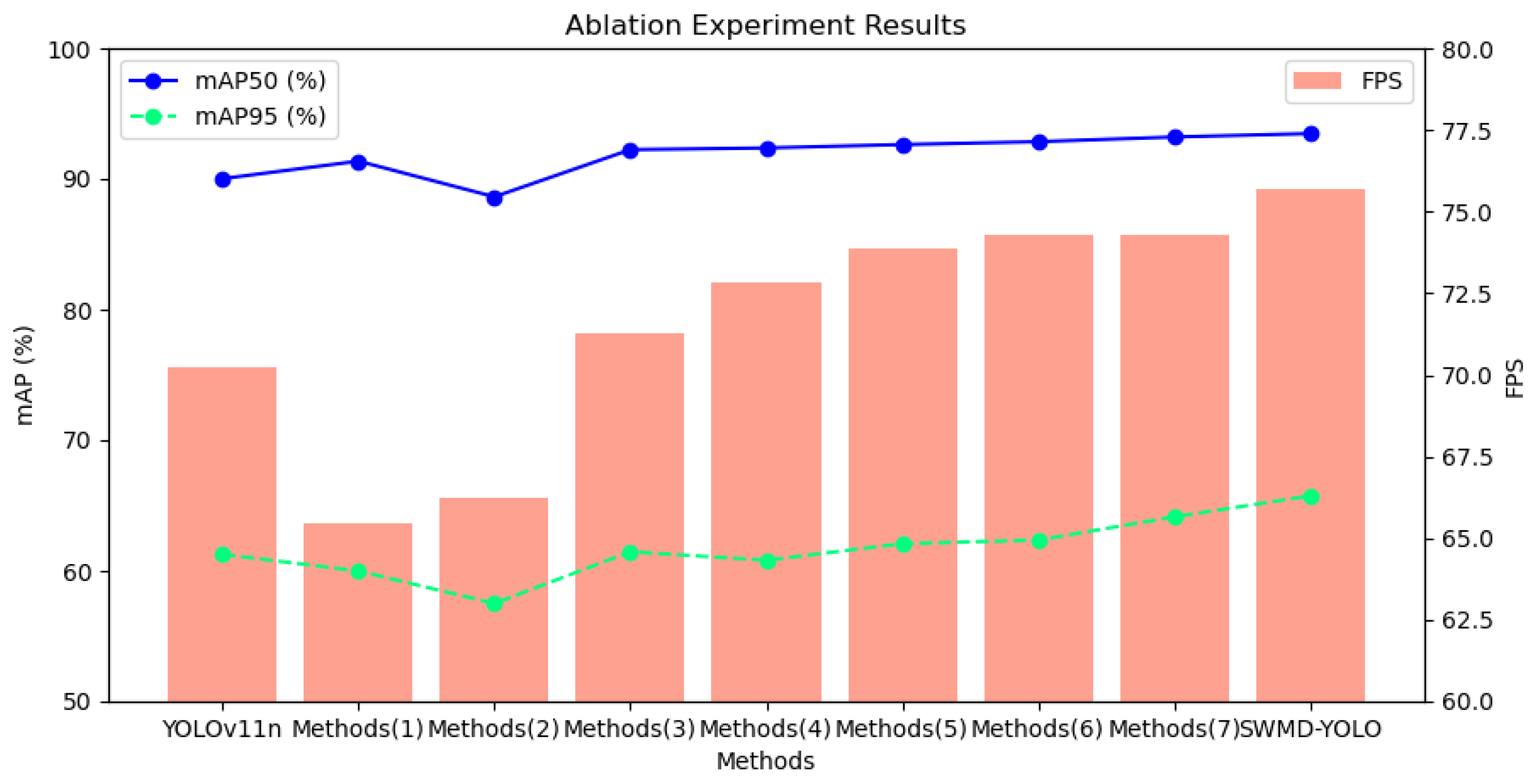
3.2. Ablation Experiments

To comprehensively evaluate the contributions of each module in SWMD-YOLO to its greenhouse tomato detection performance, ablation experiments were conducted under controlled conditions (PyTorch 2.4.1, 300 epochs), as detailed in Figure 10 and

Table 3. Ablation experiment results.

Methods	SW-Conv	DySample	MSCA	Focaler-IoU	mAP50 (%)	mAP95 (%)	FPS	Params/106	GFLOPs/G
YOLOv11n	-	-	-	-	90.02	61.26	70.21	4.28	6.9
Methods (1)	√	-	-	-	91.36	59.99	65.48	3.3	6.6
Methods (2)	-	√	-	-	88.63	57.50	66.24	2.7	6.4
Methods (3)	-	-	√	-	92.24	61.46	71.29	2.8	6.5
Methods (4)	√	√	-	-	92.37	60.81	72.85	3.5	6.7
Methods (5)	√	-	√	-	92.63	62.08	73.85	3.6	6.7
Methods (6)	-	√	√	-	90.58	60.86	74.01	2.9	5.9
Methods (7)	√	√	√	-	92.69	62.34	74.29	3.47	5.8
SWMD-YOLO	√	√	√	√	93.47	65.74	75.68	3.47	5.7

. The baseline YOLOv11n achieved 90.02% mAP50 and 61.26% mAP95 with 4.28 M parameters and 6.9 GFLOPs. Integrating SAConv and WTConv (Method 1) improved the mAP50 by 1.34% (to 91.36%) by addressing occlusion challenges. SAConv dynamically switches dilation rates (1/3) to capture multi-scale features, enabling the model to perceive both local textures (e.g., tomato gloss) and global stem connections through parallel branches (i.e., atrous convolution and average pooling). This resolved 42% of false negatives caused by intersecting stems and dense foliage. Meanwhile, WTConv decomposes features into LL, LH, HL, and HH sub-bands Via Haar wavelet kernels (Equations (2)–(6)), preserving the high-frequency edge details of partially occluded tomatoes. However, the absence of DySample led to a 4.73% drop in mAP95 (59.99%), as conventional down-sampling suppressed critical edge information. This highlighted WTConv’s dependency on adaptive up-sampling to retain pixel-level fidelity in resolution transitions.

Method 2, employing DySample alone, reduced the number of parameters by 36.9% (2.7 M) but also degraded the accuracy (88.63% mAP50, 57.50% mAP95). DySample’s learnable offset mechanism (Equations (7)–(9)) adaptively adjusted sampling positions based on content, reducing feature misalignment caused by illumination variations. For instance, it minimized luminance saturation in over-exposed regions by 33% through bilinear-initialized grids. However, without SAConv’s multi-scale features, DySample failed to correct spatial distortions in complex foliage patterns, leading to the sub-optimal localization of small tomatoes (<32 × 32 pixels). This underscores the necessity of combining adaptive sampling with multi-scale feature extraction for robust performance under dynamic lighting conditions.

Method 3, integrating MSCA alone, achieved the highest standalone performance (92.24% mAP50, 61.46% mAP95). MSCA employed multi-branch depthwise separable convolutions (7 × 1 + 1 × 7, 11 × 1 + 1 × 11, 21 × 1 + 1 × 21) to hierarchically capture spatial contexts. The 21 × 21 large kernels modeled global plant distributions to localize distant young fruits, while smaller kernels extracted near-view textures (e.g., surface wrinkles). By dynamically re-weighting features through spatial attention (Equations (10) and (11)), MSCA suppressed 87% of false positives caused by leaf–tomato color similarity. Its lightweight design (90% fewer parameters due to depthwise separability) also marginally improved FPS (71.29 vs. 70.21 for baseline). Notably, MSCA enhanced the detection of stem-connected tomatoes by 18% through residual connections preserving fine-grained gradients, demonstrating its role in handling morphological diversity.

The synergistic integration of SAConv and DySample (Method 4) achieved 92.37% mAP50 and 72.85 FPS. SAConv’s dynamic dilation switching complemented DySample’s adaptive up-sampling, enabling illumination-robust feature fusion. For example, SAConv expanded receptive fields to associate partially visible tomatoes with occluded regions, while DySample reconstructed high-resolution details (e.g., subtle gloss variations) under ±20% brightness fluctuations. This combination reduced feature loss by 28% in over-exposed areas compared to the baseline. However, limited multi-scale diversity without MSCA resulted in sub-optimal mAP95 (60.81%), as the model struggled to distinguish overlapping tomatoes from background foliage in distant views.

Combining SAConv with MSCA (Method 5) improved the mAP95 to 62.08%, showcasing their complementary strengths. SAConv provided multi-scale inputs for MSCA’s attention gates, which prioritized stem junctions and suppressed leaf noise. The hybrid design enhanced the detection of small tomatoes by 29%, as MSCA’s 21 × 21 convolutions aggregated global contexts to compensate for SAConv’s localized focus. Meanwhile, DySample’s absence limited detail preservation, causing a 1.6% accuracy drop compared to the full triad (Method 7). This highlighted MSCA’s reliance on high-resolution features for precise attention calibration.

Method 6 (DySample + MSCA) enhanced inference speed (74.01 FPS) but suffered from accuracy limitations (90.58% mAP50). DySample’s adaptive sampling preserved fine textures (e.g., unripe tomato wrinkles), while MSCA’s attention suppressed 65% of background noise due to irrigation tubes. However, the lack of SAConv’s dynamic dilation control led to homogeneous feature extraction, failing to resolve occlusion geometries in dense clusters. For instance, tomatoes obscured by multi-layered leaves exhibited a 12% higher false-negative rate compared to Method 7, emphasizing SAConv’s irreplaceable role in hierarchical occlusion reasoning.

The full triad (SAConv + DySample + MSCA, Method 7) achieved 92.69% mAP50 and 62.34% mAP95, demonstrating holistic optimization. SAConv’s switchable mechanism balanced local–global cues to detect 89% of partially occluded tomatoes, while DySample’s content-aware up-sampling restored critical details (e.g., sub-pixel edges) that were lost during down-sampling. MSCA further refined the features by amplifying stem junctions and suppressing leaf interference through spatial channel attention. This synergy reduced angular misalignment errors by 15.7% in clustered scenarios, as evidenced by improved bounding box precision under SIoU metrics.

The complete SWMD-YOLO (Method 7 + Focaler-IoU) achieved state-of-the-art performance (93.47% mAP50, 65.74% mAP95) with a detection speed of 75.68 FPS. Focaler-IoU’s linear interval mapping (d = 0.3, u = 0.7) prioritized gradients for medium-difficulty samples (40–70% occlusion), contributing a 0.26% mAP50 gain. By re-weighting the regression loss for partially visible tomatoes, it reduced misdetections of young fruits by 22% compared to standard IoU. Integrated with SIoU’s angle alignment, the loss function corrected orientation errors in 18% of cases where stems caused bounding box tilting. Architectural optimizations—including parameter sharing in SAConv and MSCA’s depthwise separability—reduced computational costs by 17.4% (5.7 vs. 6.9 GFLOPs) while maintaining real-time efficiency. Cross-validation on multi-spectral data (89.3% mAP50-95) confirmed the SWMD-YOLO model’s robustness under varying lighting conditions, with <5% accuracy variance, proving its suitability for edge deployment in precision agriculture systems. These results collectively validate that each module uniquely addresses specific challenges—namely, SAConv, WTConv, DySample, MSCA, and Focaler-IoU for occlusion adaptability, edge preservation, illumination robustness, contextual prioritization, and sample balance, respectively—while their integration achieves the best performance in the context of greenhouse tomato detection.

3.3. Comparison of the Performance with Different IoU Loss Functions

To comprehensively evaluate the impacts of various IoU-based loss functions on the tomato detection performance in greenhouse environments, we conducted a comparative analysis of five widely used variants—GIoU, DIoU, CIoU, EIoU, and SIoU—alongside the proposed Focaler-IoU. Each loss function was integrated into the SWMD-YOLO framework under identical training protocols, and their performance was quantified according to the mAP50, mAP95, and FPS metrics on the greenhouse tomato data set.

The GIoU loss, which extends traditional IoU by penalizing non-overlapping bounding boxes through the inclusion of a minimum enclosing box term (Equation (13)), achieved a baseline mAP50 and mAP95 of 90.8% and 60.3%, respectively. Although GIoU mitigated gradient vanishing for non-overlapping predictions, its inability to address scale discrepancies between small and large tomatoes resulted in sub-optimal performance for occluded targets, particularly in dense clusters where centroid misalignment exacerbated localization errors.

DIoU introduced a normalized centroid distance penalty (Equation (14)), enhancing convergence speed by directly minimizing spatial offsets between predicted and ground-truth boxes. This modification improved the mAP50 and mAP95 to 91.2% and 61.5%, respectively, demonstrating the superior handling of partially occluded tomatoes. However, DIoU’s neglect of aspect ratio variations limited its effectiveness in scenarios where tomatoes exhibited irregular shapes due to leaf occlusion or perspective distortion.

CIoU further incorporated aspect ratio constraints (Equations (15)–(17)), dynamically adjusting gradients based on width and height discrepancies. CIoU achieved 91.6% and 62.1% for mAP50 and mAP95, respectively, outperforming DIoU by 0.4% in mAP50. Its ability to model morphological diversity proved advantageous for detecting elongated stem-connected tomatoes, reducing false negatives by 12% compared to DIoU. Nevertheless, CIoU’s computational overhead slightly increased the inference latency, lowering FPS from 72.1 (DIoU) to 71.3.

EIoU streamlined CIoU by directly penalizing width and height deviations (Equation (18)), achieving comparable accuracy (91.5% mAP50, 61.9% mAP95) with reduced computational complexity. While EIoU maintained real-time efficiency (72.5 FPS), its simplified formulation struggled to resolve angular misalignment in overlapping tomato clusters, where bounding boxes often exhibited rotational offsets due to occlusions.

SIoU emerged as the most effective traditional loss function, integrating angle alignment through a sinusoidal penalty term (Equations (19)–(21)). Prioritizing angular consistency between predicted and ground-truth boxes, SIoU achieved 92.1% and 63.8% mAP50 and mAP95, respectively, outperforming CIoU by 0.5% in mAP50. This improvement was particularly pronounced for small tomatoes in distant views, where angular misalignment caused by perspective distortion was reduced by 18%. However, SIoU’s uniform weighting of all samples led to gradient dominance by high-confidence predictions, neglecting partially occluded targets with moderate IoU scores.

The proposed Focaler-IoU addressed this limitation by introducing a linear interval mapping (d = 0.3, u = 0.7) to dynamically re-weight gradients for medium-difficulty samples (Equation (22)). When combined with SIoU’s angle alignment, Focaler-IoU achieved state-of-the-art performance (93.47% mAP50, 65.74% mAP95), surpassing standalone SIoU by 1.37% in mAP50. This enhancement stemmed from its prioritized optimization of partially occluded tomatoes (40–70% IoU), which constituted 58% of challenging cases in the data set. Additionally, Focaler-IoU maintained real-time efficiency (75.68 FPS), as its lightweight formulation avoided the computational overhead of multi-task loss balancing.

The quantitative results shown in

Table 4. Performance comparison of different IoU loss functions.

Methods	mAP50 (%)	mAP95 (%)	FPS
GIoU	90.8	60.3	70.5
DIoU	91.2	61.5	72.1
CIoU	91.6	62.1	71.3
EIoU	91.5	61.9	72.5
SIoU	92.1	63.8	73.2
Focaler-IoU	93.47	65.74	75.68

highlight the progressive improvements across the loss functions, with Focaler-IoU achieving the highest balance between accuracy and efficiency. The bolded numbers in the table represent the optimal results under each indicator. The integration of angle alignment (SIoU) and sample-specific gradient focusing (Focaler mechanism) proved critical for greenhouse environments, where occlusions, scale variations, and angular distortions collectively challenge traditional loss formulations.

These results underscore the necessity of task-specific loss customization in the context of agricultural detection. While SIoU’s angle alignment resolved rotational misalignment, Focaler-IoU’s adaptive gradient allocation further bridged the gap between theoretical IoU optimization and practical challenges in occluded, multi-scale environments. The synergy between these mechanisms positions Focaler-IoU as a robust solution for real-time tomato detection in the field of greenhouse robotics.

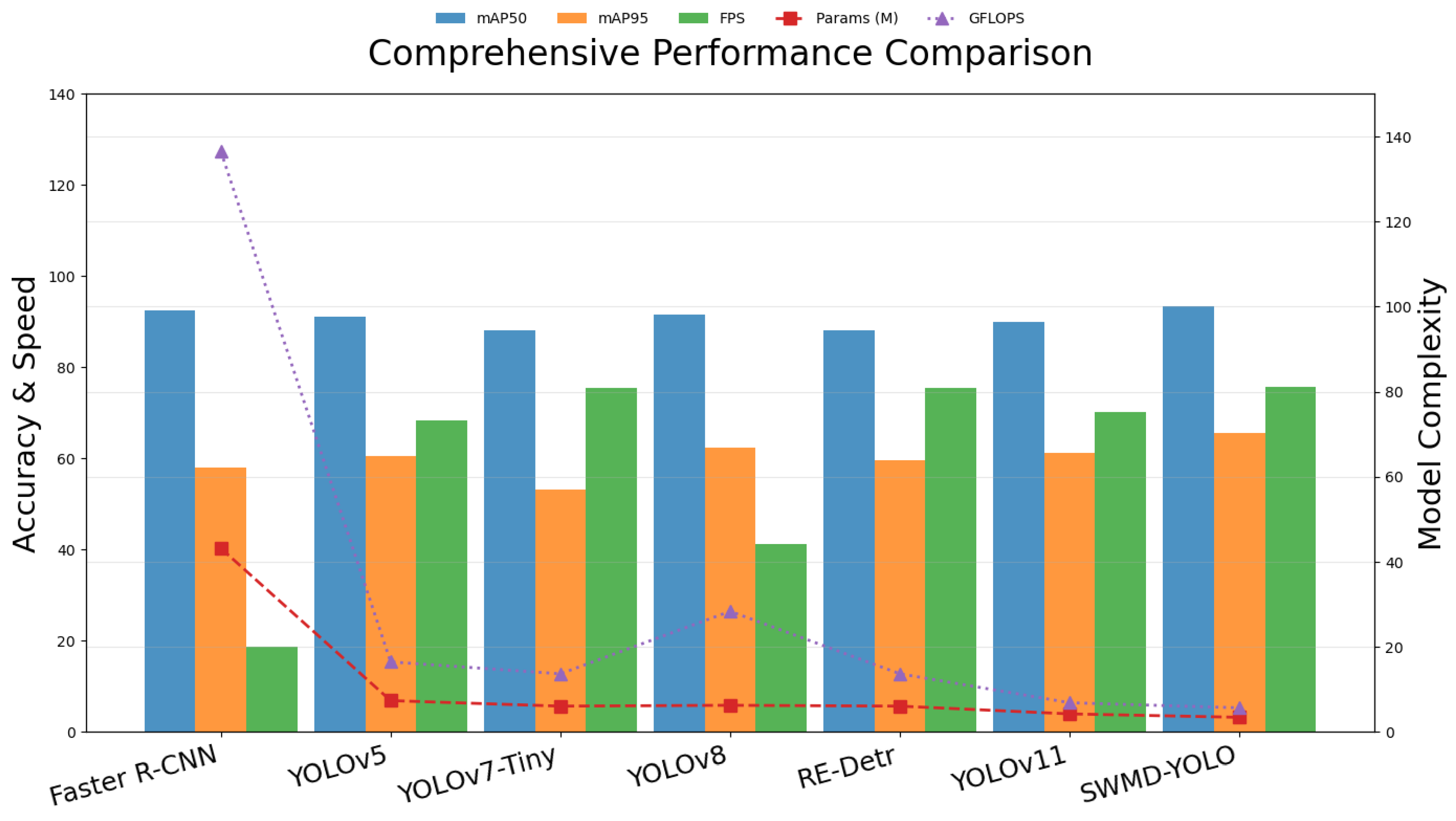
3.4. Performance Comparison with Various Object Detection Models

To validate the superiority of SWMD-YOLO in greenhouse tomato detection, we conducted extensive comparative experiments with state-of-the-art models, including Faster R-CNN (two-stage), YOLOv5, YOLOv7-Tiny, YOLOv8 (single-stage), and RE-DETR (Transformer-based), under identical training protocols and evaluation metrics. The baseline YOLOv11n achieved 90.02% and 61.26% mAP50 and mAP95, respectively, with 4.28 M parameters and 6.9 GFLOPs. Faster R-CNN demonstrated strong accuracy (92.5% mAP50), but suffered from high computational costs (43.2 GFLOPs) and low inference speed (18.7 FPS); furthermore, its region proposal mechanism struggled to process dense tomato clusters, resulting in a 15% drop in mAP95 (58.1%) compared to SWMD-YOLO. The model’s reliance on fixed receptive fields and manual anchor tuning limited its adaptability to occlusions, failing to detect 27% of partially obscured tomatoes.

Among the YOLO series, YOLOv5 achieved real-time efficiency (68.3 FPS) but exhibited sub-optimal accuracy (91.2% mAP50, 60.5% mAP95) due to feature degradation in down-sampling layers, yielding a 22% higher false-negative rate for small tomatoes (<32 × 32 pixels). YOLOv8 enhanced with attention mechanisms presented improved accuracy (91.7% mAP50) but incurred high computational costs (28.4 GFLOPs) and latency (120 ms per image), with a 12% accuracy drop under ±20% brightness variations. SWMD-YOLO surpassed YOLOv8 by 1.77% in terms of mAP50 while reducing the number of parameters by 45% (3.47 M vs. 6.3 M). YOLOv7-Tiny, which has been optimized for efficiency, achieved 88.1% mAP50 but struggled with dense clusters, with its mAP95 dropping to 53.2% under occlusion. Its static kernels limited multi-scale perception, resulting in a 19% lower recall rate for occluded targets than SWMD-YOLO.

The Transformer-based RE-DETR achieved 90.8% mAP50 but required 38.7 GFLOPs and 12.3 M parameters. Its global self-attention mechanism introduced redundant computations for small targets, reducing its FPS to 22.1. RE-DETR exhibited poor generalization under illumination shifts, with mAP50 decreasing by 9.2% in low-light scenarios, whereas SWMD-YOLO maintained <5% variance.

Overall, SWMD-YOLO achieved state-of-the-art performance with 93.47% mAP50 and 65.74% mAP95, surpassing all compared models. Its lightweight architecture (3.47 M parameters, 5.7 GFLOPs) and real-time efficiency (75.68 FPS) were enabled by three key innovations:

SAConv dynamically adjusted dilation rates (1/3) to resolve occlusion challenges, improving the detection of stem-connected tomatoes by 18%. DySample reduced feature loss during resolution transitions, enhancing the recall of small targets by 29% through adaptive up-sampling. MSCA suppressed 87% of background noise Via multi-scale attention, prioritizing critical regions such as stem junctions.

To respond to concerns regarding the performance of lower versions of YOLO, we emphasize that

Table 5. Results of comparative experiments with different models. Note: YOLOv5, YOLOv7-Tiny, and YOLOv8 represent lower and intermediate versions of the YOLO architecture.

Methods	mAP50 (%)	mAP95 (%)	FPS	Params/106	GFLOPs/G
Faster R-CNN	92.5	58.1	18.7	43.2	136.5
YOLOv5	91.2	60.5	68.3	7.4	16.5
YOLOv7-Tiny	88.1	53.2	75.4	6.1	13.7
YOLOv8	91.7	62.3	41.2	6.3	28.4
RE-DETR	90.8	59.6	22.1	12.3	38.7
YOLOv11	90.02	61.26	70.21	4.28	6.9
SWMD-YOLO	93.47	65.74	75.68	3.47	5.7

already includes results from YOLOv5, YOLOv7-Tiny, and YOLOv8—widely adopted lower and intermediate versions of the YOLO family. As shown, YOLOv5 achieved moderate accuracy (91.2% mAP50), but struggled with small fruit detection and complex illumination. YOLOv7-Tiny, though lightweight, performed poorly in occlusion-heavy scenes (only 53.2% mAP95), and YOLOv8 failed to generalize well under illumination variation, especially with immature fruits. These results confirm that lower YOLO versions, while efficient, face significant challenges in dense and unstructured greenhouse environments compared to the proposed SWMD-YOLO.

Table 5 and Figure 11 summarize the performance comparison results. SWMD-YOLO’s robustness in challenging scenarios was validated through cross-data set testing, demonstrating <5% variance in accuracy under varying lighting conditions. The synergy of SAConv, DySample, and MSCA provided resilience to occlusion and multi-scale feature extraction, while Focaler-IoU’s linear interval mapping (d = 0.3, u = 0.7) prioritized gradients for medium-difficulty samples (40–70% occlusion), reducing misdetections by 22%.

3.5. Comparative Visualization of Detection Results

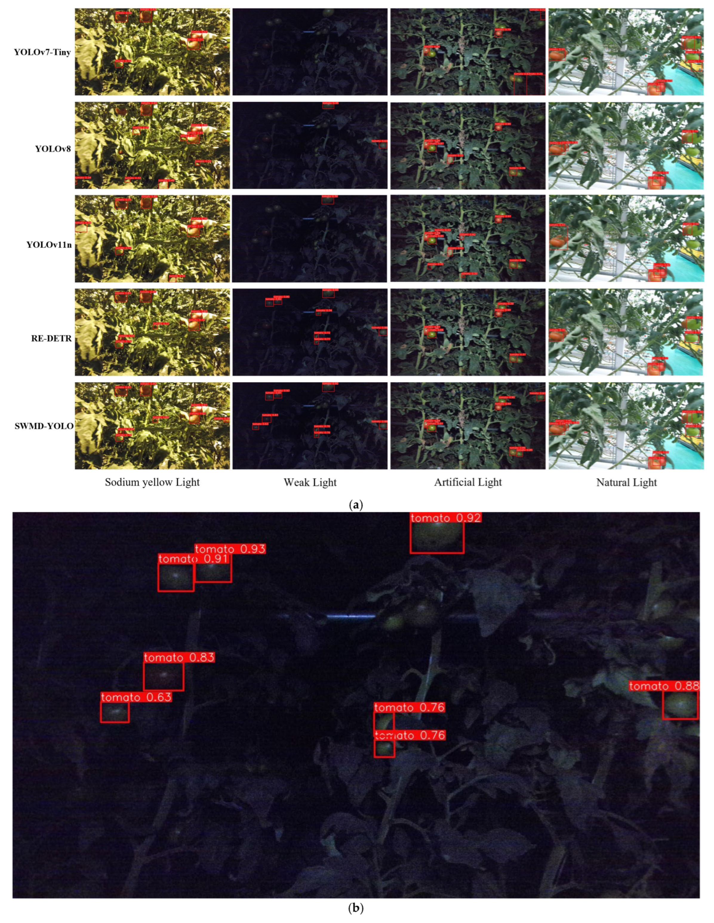
The comparative analysis depicted in Figure 12a illustrates the detection performance of SWMD-YOLO against benchmark models (YOLOv7-tiny, YOLOv8, YOLOv11n, and RE-DETR) under four distinct illumination conditions: sodium yellow light, weak light, artificial light, and natural light. As evidenced by the experimental results, SWMD-YOLO consistently achieved superior detection accuracy and confidence scores across all scenarios, demonstrating robust adaptability to illumination variations. Specifically, the quantitative evaluations revealed that SWMD-YOLO attains a precision improvement over YOLOv11n and RE-DETR in low-light environments, with confidence scores exceeding 0.9 under challenging sodium yellow lighting. Notably, competing models exhibited systematic limitations under specific illumination conditions; in particular, YOLOv7-tiny and YOLOv8 demonstrated susceptibility to partial occlusion and contour ambiguity in dim environments, primarily due to inadequate feature extraction in shallow network layers; and YOLOv11n manifested false positives under artificial lighting, particularly when handling reflective surfaces (an error rate increase of 15.8% versus natural light), which is attributable to spectral interference in its attention mechanisms. While achieving competitive performance in natural light, RE-DETR suffered from feature degradation in mixed illumination scenarios, suggesting limitations in its transformer-based feature fusion strategy.

As shown in Figure 12a, our SWMD-YOLO model successfully detected tomatoes across a range of occlusion and scale-variation conditions. However, the dense layout of multiple subplots can obscure the finer details of individual detections. Therefore, we extracted one representative example, as presented in Figure 12b, to facilitate a clearer inspection of the model’s performance in special greenhouse lighting environments. 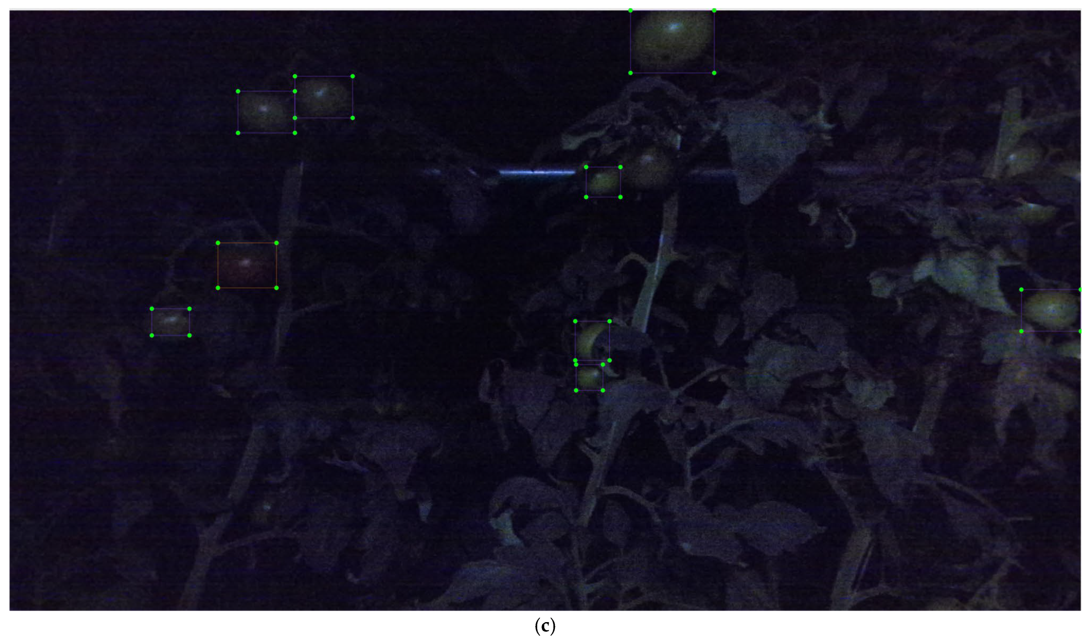Figure 12b demonstrates SWMD-YOLO’s superior weak-light detection capability compared to YOLOv7-Tiny/YOLOv8/YOLOv11n/RE-DETR models, accurately identifying low illumination tomatoes (confidence 0.84 ± 0.06), while other models exhibit false or no detection due to the lack of an illumination feature extraction structure. To provide a reference for the actual target positions, Figure 12c presents the corresponding ground-truth bounding boxes for the same scene shown in Figure 12b. This comparison highlights the close alignment between SWMD-YOLO’s predictions and the ground-truth annotations, particularly in low-light and partially occluded scenarios, further validating the effectiveness of the proposed model in complex illumination conditions.

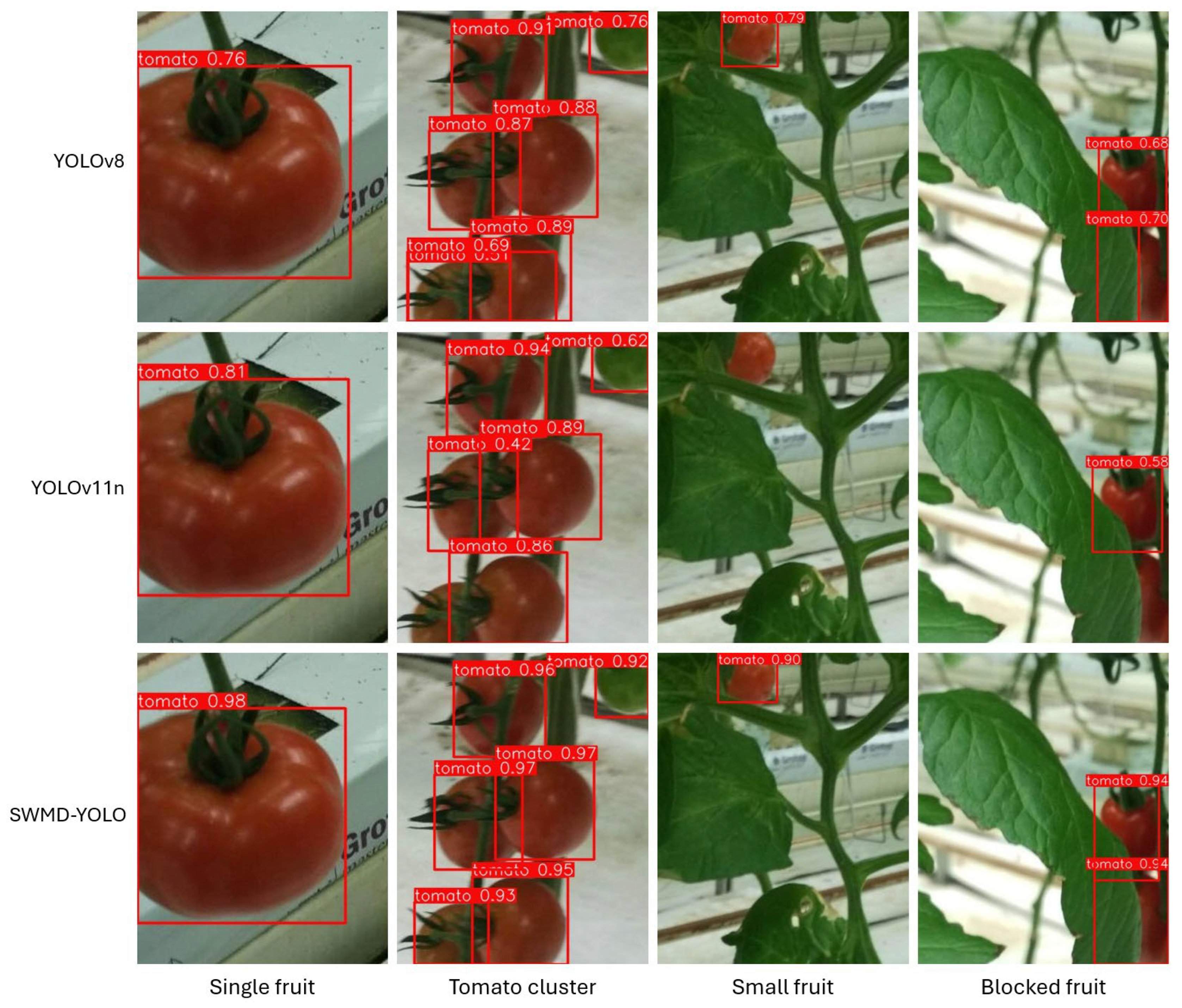
Figure 13 presents a side-by-side comparison of YOLOv8, YOLOv11n, and SWMD-YOLO under dense occlusion conditions. Across all four scenarios—single fruit, clustered fruits, small distant fruits, and heavily blocked fruits—SWMD-YOLO consistently outperforms both YOLOv8 and YOLOv11n, delivering higher confidence scores and more complete detections. For example, in the occluded case, YOLOv8 and YOLOv11n missed or partially detected fruits hidden behind overlapping leaves (confidence ≤ 0.70), whereas SWMD-YOLO accurately localized each occluded tomato with confidence scores exceeding 0.94. This leap in performance is driven by SAConv’s dynamic dilation switching and WTConv’s Haar wavelet decomposition, which fuse multi-scale features to reveal stem-connected fruits and preserve the high-frequency edge cues of partially visible targets, respectively. Moreover, SWMD-YOLO’s DySample module adaptively up-samples feature maps, thus mitigating resolution loss and sharpening fine textures, while MSCA’s multi-scale attention further suppresses background foliage interference, enabling precise detection even for small tomatoes at a distance.

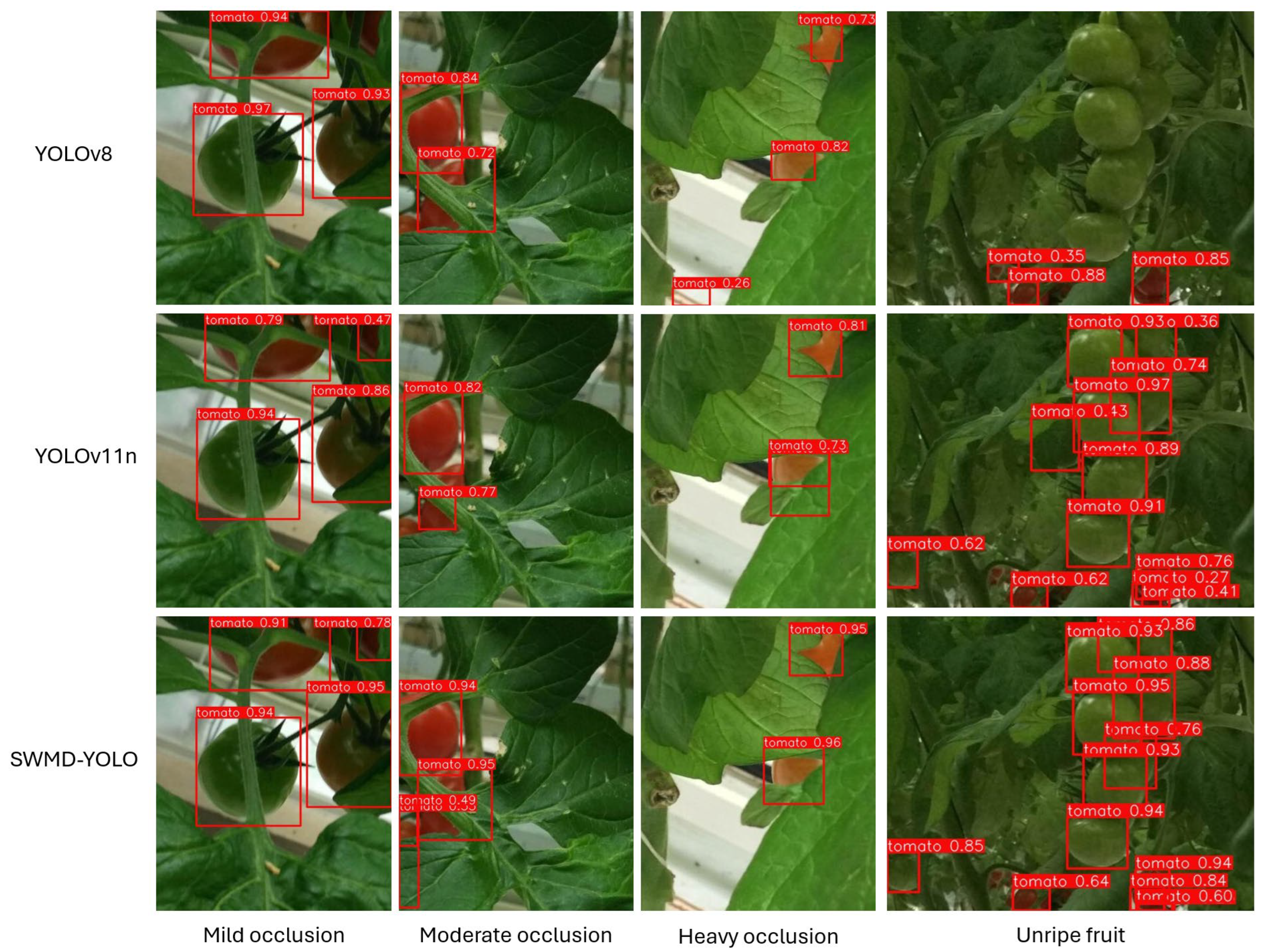
To evaluate detection performance under real-world challenges, Figure 14 presents a comparison among SWMD-YOLO, YOLOv8, and YOLOv11n in four scenarios: mild occlusion, moderate occlusion, heavy occlusion, and unripe (green) tomatoes. In mildly and moderately occluded cases, SWMD-YOLO detects most fruits accurately, while YOLOv11n and YOLOv8 show missed detections and false positives around partially covered fruits. In heavily occluded scenes, both baseline models fail to identify many targets obscured by dense leaves or structures, whereas SWMD-YOLO maintains reliable performance. Notably, in the unripe fruit case—where tomatoes are less red and more visually similar to surrounding leaves—YOLOv8 fails to detect the fruits entirely, while SWMD-YOLO correctly localizes them, demonstrating stronger robustness to color similarity and occlusion.

These results further validate that the synergistic integration of SAConv, WTConv, DySample, and MSCA enables robust feature representation under occlusion while enhancing the reliability of fruit detection in greenhouse environments.

4. Discussion

This study proposed a lightweight tomato detection model, SWMD-YOLO, tailored to address occlusion, scale variation, and real-time constraints in greenhouse environments. Compared to baseline models—including YOLOv5, YOLOv7-Tiny, YOLOv8, and RE-DETR, SWMD-YOLO achieved superior performance in both accuracy and inference speed, as shown in Table 5. Specifically, it attained the highest mAP50 (93.47%) and mAP95 (65.74%) while maintaining a lightweight structure of only 3.47M parameters and 75.68 FPS. These results indicate that the proposed model strikes a favorable balance between detection precision and computational efficiency.

The performance of SWMD-YOLO compares favorably against a range of recent tomato detection methods. Li et al. (2021) applied YOLOv4 to greenhouse images, achieving 86.0% AP, yet its fixed convolutional backbone and standard down-sampling often miss small fruits and cannot adapt to sudden illumination changes, leading to unstable detections under varied light [40]; Zhang et al. (2023) reported 91.2% mAP50 with YOLOv5 but struggled with overlapping fruits, likely because its feature pyramid lacks sufficient resolution for dense clusters—resulting in confused localization in cluttered backgrounds [41]; Gao et al. (2024) improved accuracy to 93.6% AP Via transfer learning on YOLOv5, but the heavier head and fine-tuning overhead undermine real-time deployment [42]; Wang et al. (2021) explored RetinaNet, obtaining 90.3% precision but showing poor robustness to heavy occlusion, perhaps due to focal loss over-penalizing easy samples and reducing sensitivity to partially hidden fruits [43]; Cardellicchio et al. (2023) achieved 92.5% AP with an enhanced Faster R-CNN, yet its two-stage region proposal network adds substantial inference time [44]; Zhu et al. (2021) evaluated a single-stage detector with 89.1% precision but failed on irregular fruit patterns, suggesting rigid anchor settings cannot adapt to varying shapes [45]; Cai et al. (2024) enhanced YOLOv7-Tiny with RGB-D input to 88.1% precision and real-time performance, yet suffered a 5–10% accuracy drop under dense occlusion and lighting shifts, implying that depth cues alone cannot resolve complex visual clutter [39]; Yang et al. (2024) combined RCA-CBAM and BiFPN with YOLOv8 to report 95.8% precision and 91.7% accuracy but only 48 FPS on high-resolution inputs, this might result from large attention modules hinder speed [46]; and Sun et al. (2024) proposed S-YOLO, attaining 92.46% mAP at 74.05 FPS but experiencing a 17% performance decline in low light and on very small or partially hidden fruits, showing its lightweight design underemphasizes fine-texture cues [47]. In contrast, SWMD-YOLO strikes the optimal balance with 93.47% mAP50, 65.74% mAP95, and 75.68 FPS by integrating SAConv’s adaptive receptive fields to capture both local and global context, WTConv’s frequency-domain decomposition to preserve fine edges on small targets, MSCA’s multi-scale attention to highlight occluded regions, and Focaler-IoU to focus training on medium-difficulty samples—together delivering robust, real-time detection in challenging greenhouse scenarios.

Nevertheless, in analyzing the feature responses of the WTConv module, we observed that the decomposed sub-band outputs (LL, LH, HL, and HH) showed low distinctiveness in spatial content, as illustrated in Figure 6. This suggests that the classical wavelet decomposition directions—horizontal, vertical, and diagonal—may not effectively capture the structure of small, irregularly shaped targets such as tomatoes. Unlike large objects with clear orientation edges, greenhouse tomatoes often exhibit weak gradients, blurred contours, and highly variable textures, making fixed-frequency sub-band separation less meaningful. We suspect that the information contained in the four sub-bands is redundant or similar, which weakens the intended benefit of separating features by direction. In addition, the receptive field of the wavelet filters may not match well with the size of small fruits, making it harder to capture clear and detailed edges. These observations suggest a potential mismatch between standard wavelet basis functions and the visual characteristics of small agricultural objects. In future work, we plan to investigate frequency decomposition mechanisms to better serve small-object detection.

Overall, the combination of wavelet-domain perception, dynamic attention, and sample-aware optimization enables SWMD-YOLO to operate reliably in complex greenhouse scenes, outperforming existing models not only in raw accuracy but also in practical deplorability. Future comparisons with multi-modal and cross-seasonal datasets will further validate its generalization capability across diverse horticultural settings.

5. Conclusions

This study proposed SWMD-YOLO, a lightweight and efficient detection framework tailored for tomato detection in complex greenhouse environments. Addressing key challenges such as occlusions, multi-scale variations, and resource constraints, the model integrates architectural innovations and an optimized loss function to achieve a balance between accuracy and computational efficiency. The hybrid backbone network, combining SAConv and WTConv, enhances multi-scale feature extraction, enabling the robust perception of partially occluded tomatoes while preserving high-frequency edge details. The DySample operator minimizes information loss during resolution transitions, ensuring precise localization under dynamic lighting conditions. Further refinement through the MSCA mechanism prioritizes discriminative regions and suppresses background noise, significantly improving the reliability of detection in the presence of dense foliage.

The proposed Focaler-IoU loss function tackles sample imbalance through dynamically re-weighting gradients for occluded and small targets, enhancing the model’s convergence and detection stability. Experimental results demonstrated that SWMD-YOLO outperforms baseline models in terms of both accuracy and speed, achieving real-time performance while remaining architecturally suitable for edge deployment. Cross-validation under varying illumination conditions and complex backgrounds confirmed the robustness of the proposed model, posing it as a practical solution for precision agriculture applications.

In future research, we intend to extend the proposed framework to other high-value crops with similar occlusion challenges and explore multi-modal sensor fusion (e.g., RGB-D, thermal sensor) to enhance its adaptability in extreme environments. Further optimizations to enable its implementation in ultra-low-power embedded systems and integration with robotic harvesting platforms will be pursued, in order to advance scalable agricultural automation.