Prediction of Spatial Winter Wheat Yield by Combining Multiscale Time Series of Vegetation and Meteorological Indices

Abstract

In the context of climate change and the development of sustainable agricultural, crop yield prediction is key to ensuring food security. In this study, long-term vegetation and meteorological indices were obtained from the MOD09A1 product and daily weather data. Three types of time series data were constructed by aggregating data from an 8-day period (DP), 9-month period (MP), and six growth periods (GP). And we developed the yield prediction model by using random forest (RF) and long short-term memory (LSTM) networks. Results showed that the average root mean squared error (RMSE) of the RF model in each province was 0.5 Mg/ha lower than that of the LSTM model. Both the RF and LSTM prediction accuracies increased with the later growth stages data. Partial dependence plots showed that the influence degree of DVI on yield was above 2 Mg/ha. When the time length of the feature variables was shortened to MP or GP, the growing degree days (GDD), average minimum temperature (AveTmin), and effective precipitation (EP) showed stronger nonlinear relationships with the statistical yields.

1. Introduction

Wheat is an important grain crop in China, and the accurate prediction of wheat yield is highly important for ensuring food security, formulating agricultural policies, and stabilizing market prices [1,2,3]. There are two main methods used for yield prediction. One is a crop growth model based on the physiological and ecological processes of crops, which can describe the relationships between crop growth and environmental factors in detail, reflect the internal mechanism of crop growth, and provide high explanatory power for prediction results. However, there are several problems with this model, including too many parameters in the model process and complicated calculations [2,4,5]. The second approach builds a data-driven model and uses multiple linear regression, deep learning, machine learning, and other methods to find potential correlation patterns, trends, and correlations from big data without understanding the complex and nonlinear mechanism processes inside the system, effectively improving modeling efficiency. However, quality problems such as errors, missing values, deviations, and noise in the data can significantly affect the accuracy of yield prediction [1,6].

A variety of machine models, such as recurrent neural networks (RNN), random forest (RF), and long short-term memory (LSTM) networks, have been applied to time-series data modeling, including agricultural planting structure extraction, yield prediction, and disease and pest prediction, as they are capable of handling the inherent nonlinearity in the feature variables [7,8]. In addition, because natural environment data are important data for modeling and have continuity in time, the modeling of time series data has also been applied to generate data with high temporal resolution, such as daily land-surface temperature data [9,10,11,12]. Previous studies have extensively utilized environmental data, such as meteorological and soil conditions, along with remote-sensing vegetation indices, such as the normalized difference vegetation index (NDVI) and leaf area index (LAI), as feature variables in models to quantify the impact of weather on vegetation, assess vegetation health and productivity, and predict crop yields [10,11]. Generally, the vegetation index is positively correlated with yield. In the early stage, vegetation index changes have obvious effects on yield, and in the later stage, it is affected by a variety of factors, and vegetation index often affects yield together with meteorological, soil water volume, and other factors [10]. Moreover, low-altitude remote sensing data, combined with a variety of data processing and modeling methods, including data assimilation, have been employed to obtain more precise phenotypic data, which have been combined with field yield predictions for more accurate forecasting [4,10,13,14]. In addition, the accuracy of deep learning in crop yield prediction is greater than that of traditional machine-learning methods, and the model generalizability is strong. However, crop yield is a highly complex trait that is affected by many factors, such as environmental conditions and crop genotype, and a complex model is needed to reveal the functional relationships between these interactive factors and crop yield [4,15].

Most of the time-series data required for crop yield prediction come from sensor monitoring data, including meteorological, soil, and satellite remote-sensing data, which also include day-by-day and even hour-by-hour weather data generated by weather research and forecasting systems [3,16,17]. Owing to the stability of the physical and chemical properties of the soil itself, soil temperature and moisture content with high temporal resolution can be obtained by soil sensors in small areas and by multispectral and microwave data inversion of satellite sensors, such as Sentinel-1, Sentinel-2, Sentinel-3, and AMSR2, over large areas [18,19]. However, remote-sensing image data are often affected by cloud coverage, resulting in missing pixel values. To address the missing pixels, various algorithms can be used to re-establish image time series [20,21]. Alternatively, cloud-free remote-sensing imagery products, such as MOD09A1, can be used to generate vegetation indices in time series to reflect the seasonal changes in crop growth [22]. Using long time-series data, a yield prediction model could capture more long-term trends and periodic fluctuations in historical crop growth and the environment, effectively improving the generalizability of the yield prediction model in different years and regions. However, there will be more data redundancy, resulting in greater training time and computing resource consumption. If the time series of environmental data required for modeling is short, the yield prediction model will be too sensitive to random fluctuations in the data, and occasional fluctuations will be added to the model as a long-term trend, resulting in low prediction accuracy [4]. Moreover, the generalizability of the yield prediction model is affected by the training dataset, and the model may not adapt appropriately to new, unseen time-series data [17]. Previous studies used 789 daytime and nighttime MODIS LST products for land-surface temperature prediction with LSTM models [9]. In crop yield prediction studies, corn can be divided into five growth stages, namely, planted to emerge, emerged to silking, silking to dough, dough to dent, and dented to mature [22]. Feature variables have been constructed on the basis of meteorological data and satellite image data from each growth period, and multiple machine-learning methods have been used to predict U.S. maize yield [22]. In addition, at the field scale, due to the high spatial resolution of UAV, the time-series spectral index can be constructed by combining crop canopy attributes and vegetation index to predict crop yield [23]. However, few studies have investigated the effects of different time-series lengths on model accuracy.

In this study, we constructed a variety of time-series data using meteorological indices and vegetation indices. We used RF and LSTM methods to establish a yield prediction model for China’s winter wheat area to verify whether a higher temporal resolution of time series data leads to better modeling accuracy and whether the LSTM model was superior to the RF model. Finally, the appropriate time length of the feature variables for constructing the yield model and the key time points for predicting yield in advance were obtained. Our research aimed to provide methods for the application of machine learning in crop yield prediction.

2. Materials and Methods

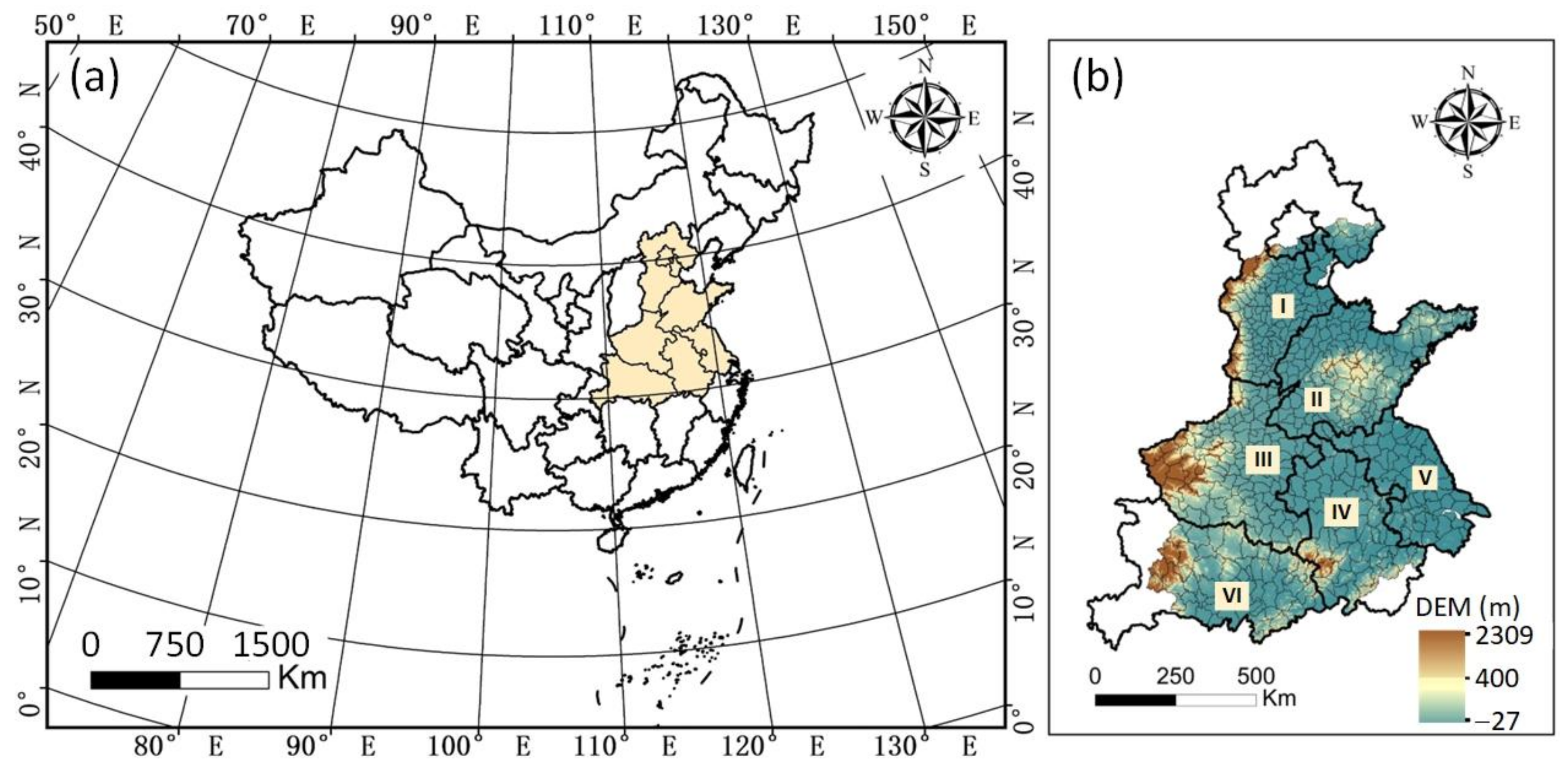
2.1. Study Area

The main production areas of winter wheat in China (110°36′ to 122°11′ E, 29°4′ to 41° 10′ N) included six provinces: Hebei, Shandong, Henan, Anhui, Jiangsu, and Hubei (Figure 1a,b). The climate types included a temperate continental monsoon climate, a warm temperate monsoon climate, an East Asian monsoon climate, a warm temperate semi-humid monsoon climate, a subtropical monsoon humid climate, and rain and heat during the same season. The annual precipitation in Hebei Province is approximately 500 mm, and that in other provinces is approximately 1000 mm. The landforms include plains, hills, and mountains. There is a significant difference in elevation between east and west, with the highest elevation being 2309 m and the lowest elevation being −27 m (Figure 1b).

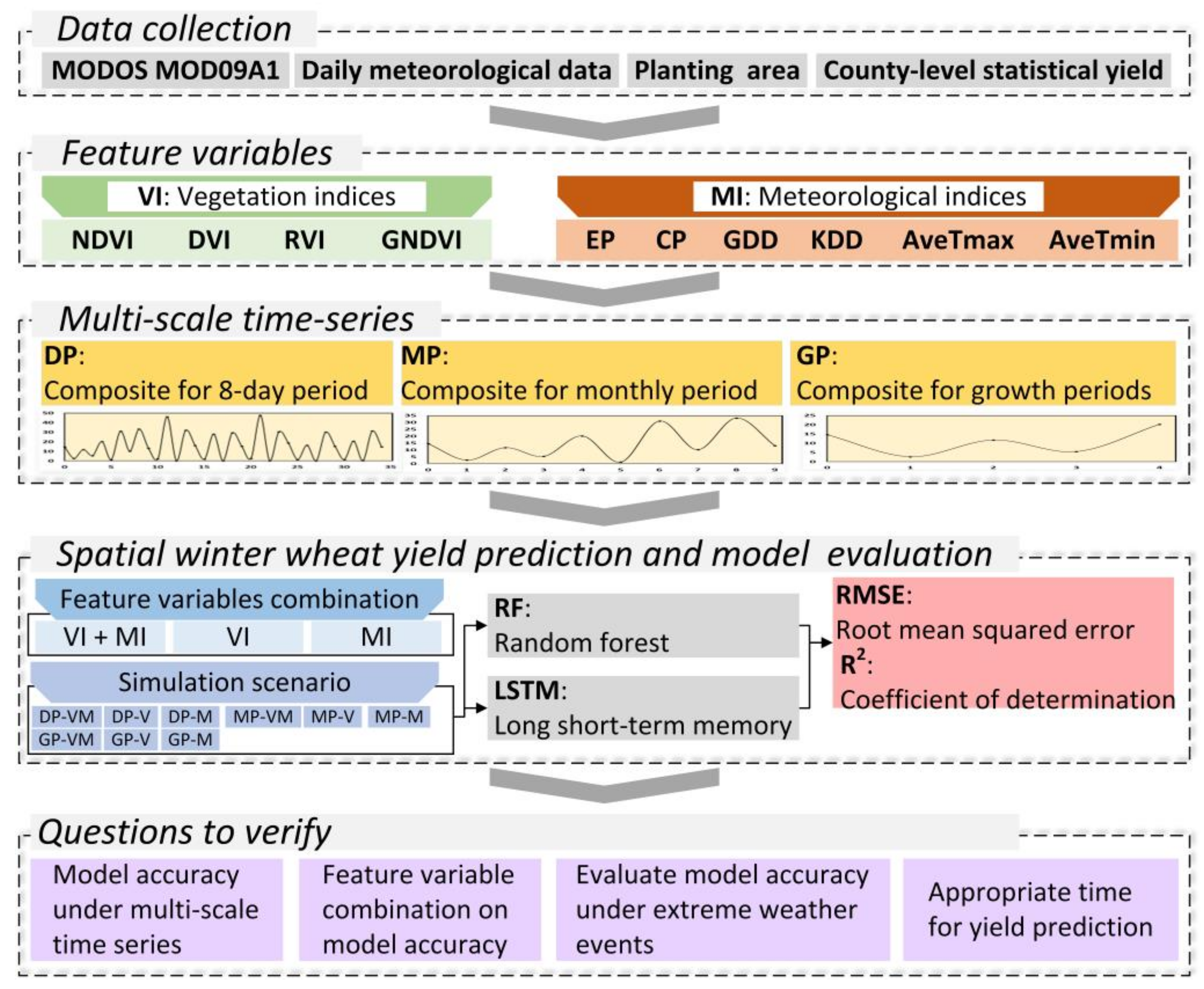
2.2. Analysis Workflow

In this study, vegetation indices and meteorological indices were used to establish feature variables, and the effects of multiple time-scale feature variables on regional winter wheat yield simulations were studied (Figure 2), which included the following six steps:

(1) The remote-sensing vegetation indices, meteorology, planting area distribution, and yield data required for this study were collected (

Table 1. Data sources and descriptions required for this study. Tmax, maximum temperature; Tmin, minimum temperature; PRE, precipitation; DEM, digital elevation model.

Data Type	Element	Format	Source	Time Resolution	Spatial Resolution
Administrative	County	shp	National Earth System Science Data Center (www.geodata.cn (accessed on 1 January 2024))	/	/
Meteorology	Tmax, Tmin, and PRE	tiff	Data Publisher for Earth & Environmental Science (https://pangaea.de/ (accessed on 19 December 2023))	Daily	1 km
Yield	Statistical yield	csv	Chinese Economic and Social Big DataResearch Platform(https://data.cnki.net/ (accessed on 1 April 2022))	Yearly	/
Remote sensing	R, G, B, near infrared	tiff	MODIS Surface Reflectance products, Google Earth Engine (https://earthengine.google.com/ (accessed on 1 January 2024))	8 days	500 m
Terrain	DEM	tiff	SRTMGL1_003 DEM (https://lpdaac.usgs.gov/products/srtmgl1v003/ (accessed on 19 December 2023))	/	30 m
Others	Planting area	tiff	National Ecosystem Science Data Center (https://www.nesdc.org.cn/ (accessed on 1 May 2024)) [24]	/	10 m

).

(2) Using remote-sensing data and meteorological data, the vegetation indices and meteorological indices, which are closely related to yield, were calculated, and the feature variables were established.

(3) The feature variables were synthesized via three types of time series, including the day period (DP), month period (MP), and growth period (GP).

(4) Three combinations of feature variables, namely, vegetation indices and meteorological indices (VI+MI), a single vegetation index (VI), and a single meteorological index (MI), were utilized to construct nine simulation scenarios with three different time series.

(5) Training data from 2014–2018 were utilized for training the RF and LSTM models, and validation data from 2019 were used to compute the root mean squared error (RMSE) and R².

(6) Finally, four results were obtained through an analysis of the model accuracy. First, by comparing the modeling accuracy of multiple time-scale data, the appropriate machine-learning method and time scale for yield simulation were obtained. Second, the influence of combining the vegetation indices and meteorological indices on the model prediction accuracy was studied. Third, the machine-learning model was verified, which was better for extreme climate simulation results. Fourth, the appropriate time point for winter wheat yield prediction was obtained.

2.3. Data Description

2.3.1. Data Collection and Preprocessing Steps

(1) Spatial data, including administrative divisions and environmental and yield data, are shown in Table 1. The study area is shown in Figure 1b, and the time range was 2014–2019 (Section 2.2).

(2) To ensure that the environmental data required for modeling are highly representative of the crop growth environment, the wheat-planting area was used to mask the meteorological data and MOD09A1. First, tiff-format planting area data were converted to shapefile data as mask files. The ExtractByMask tool in ArcMap (https://desktop.arcgis.com/zh-cn/arcmap/latest/tools/spatial-analyst-toolbox/extract-by-mask.htm (accessed on 10 May 2024)) and the clip tool of GEE (https://developers.google.com/earth-engine (accessed on 15 May 2024)) were subsequently used to extract the meteorological data and MOD09A1 data, respectively.

(3) Using the zonal statistical tool in ArcMap, the county-level administrative unit was taken as the basic spatial unit (BSU), the csv format mean statistics of all raster spatial data were obtained, and the UpdateCursor tool in ArcGIS was used to add the attribute data to the corresponding spatial unit.

(4) Finally, the vegetation indices and meteorological indices of each county were calculated to establish the model training data.

2.3.2. Calculation of Vegetation Indices

Because the time range of this study covers the whole growth period of crops, the use of a single vegetation index has limitations and cannot reflect the real situation of crop growth during the whole growth period, especially when the coverage was weak in the early growth period of crops. Therefore, in addition to the commonly used NDVI, this study selected the DVI, which is sensitive in the early stage of crop growth, and the RVI and GNDVI, which are sensitive in areas with high vegetation coverage [7,14,15].

All the vegetation indices were calculated pixel by pixel via the MOD09A1 product. The calculation formula was as follows, where N is the reflectance of the near-infrared band, $R$ is the reflectance of the red band, and G is the reflectance of the green band.

$$NDVI={\displaystyle \frac{N-R}{N+R}}$$

(1)

$$DVI=N-R$$

(2)

$$RVI=N/R$$

(3)

$$GNDVI={\displaystyle \frac{N-G}{N+G}}$$

(4)

2.3.3. Calculation of Meteorological Indices

The meteorological indices selected in this study include EP, CP, GDD, and KDD. EP refers to the amount of natural precipitation that excludes surface runoff, deep seepage, and evaporation, leaving the portion that can be absorbed by plant roots. EP plays an important role in promoting seed germination, root development, photosynthesis maintenance, yield, and quality improvement during the whole growth period of crops [25,26]. The calculation formula is as follows, where $P$ represents the total daily precipitation:

$$EP=\left\{\begin{array}{ll}4.17+0.1P& (P\ge 8.3mm/d)\\ {\displaystyle \frac{P(4.17-0.2P)}{4.17}}& (P<8.3mm/d)\end{array}\right.$$

(5)

CP refers to the cumulative value of the total amount of precipitation in a specific period. The calculation formula is as follows:

$$CP=\sum P$$

(6)

During the growth cycle of crops, sufficient heat accumulation is crucial for crop growth and yield formation. The number of GDD can be used to evaluate the effective heat accumulation experienced in a certain growth stage, and it represents the heat resources of crops during the growth period. During the vegetative growth stage, an increase in GDD is conducive to the growth of vegetative organs, such as leaves and stems. With the accumulation of GDD, the photosynthesis time of crops is prolonged, and the accumulation of photosynthetic products increases, which provides a material basis for panicle development in the reproductive growth stage and is conducive to increasing yield [7,27]. The calculation formula is as follows, where $T_{base}$ represents the basic minimum temperature for winter wheat development, with a value of 0:

$$GDD={\displaystyle \frac{T_{\max }+T_{\min }}{2}}-T_{base}$$

(7)

When the temperature exceeds the appropriate temperature during the growth period of wheat, it has adverse effects on growth, especially during the filling period. High temperatures accelerate the aging rate of wheat plants, decrease the photosynthetic function of leaves in advance, reduce the transport of photosynthetic products to grains, and even block the transport channel of photosynthetic substances, ultimately leading to a decrease in yield. The KDD is a heat index that characterizes high-temperature disasters during the crop growth period [28], where $T_{\max }$ represents the daily maximum temperature, $T_{\min }$ represents the daily minimum temperature, $T_{base}$ represents the lower-limit temperature of winter wheat growth (0 °C), and $T_{high}$ represents the upper-limit temperature (30 °C). The calculation formula is as follows:

$$KDD=\left\{\begin{array}{ll}{T}_{\max }-T_{high}& (T_{\max }>T_{high})\\ 0& (T_{\max }\le T_{high})\end{array}\right.$$

(8)

2.3.4. Construction of Multiple Time-Series Data

In this study, multiscale time series were used to composite feature variables, and each period was called a time step. In each time step, the composite method of the vegetation indices calculates the mean value in each time step, and the composite method of the meteorological indices calculates the sum in each time step. The three time-series composite methods are as follows:

(1) The MODIS product MOD09A1 was used as the basis to obtain 8 days of synthetic data. According to the date of the MODIS image-synthesis time, a total of 8 days before and after the synthesis of the meteorological indices were synthesized. For example, for an image synthesis time of the MOD09A1 product of 19 December 2019, 8 days (16 December, 17 December, 18 December, 19 December, 20 December, 21 December, 22 December, and 23 December) of daily meteorological data were synthesized, and time-series data containing 34 time steps were obtained. The annual remote-sensing image times are shown in the table below (

Table 2. MODIS remote-sensing image-acquisition time.

Harvest Year	MODIS Image Time
	Start Date	End Date	Time Interval	Image Number
2014	8 October 2013	26 June 2014	8 days	34
2015	8 October 2014	26 June 2015
2016	8 October 2015	25 June 2016
2017	7 October 2016	26 June 2017
2018	8 October 2017	26 June 2018
2019	8 October 2018	26 June 2019

).

(2) According to the growth time of winter wheat, the vegetation indices and meteorological indices were synthesized from October to June of the following year for a total of 9 months, so time-series data including nine time steps were finally obtained. These months include October, November, December, January, February, March, April, May and June.

(3) The growth period of winter wheat mainly includes the sowing stage, seedling stage, tillering stage, overwintering stage, greening stage, rising stage, jointing stage, booting stage, heading stage, flowering stage, filling stage, and maturity stage. Each growth period is approximately 21 days [29]. In this study, each growth period of winter wheat was divided into time steps, namely, the seedling–emergence period (GP1), tiller–overwintering period (GP2), greening–rise period (GP3), jointing–booting period (GP4), heading–flowering period (GP5), and filling–maturity period (GP6) (

Table 3. Start date and end date of each growth period. Oct., October; Nov., November; Dec., December, Feb., February; Mar., March; Apr., April; Jun., June.

Harvest Year	Growth Period
	GP1	GP2	GP3	GP4	GP5	GP6
2014	1 Oct. 2013– 11 Nov. 2013	12 Nov. 2013– 22 Dec. 2013	23 Dec. 2013– 1 Feb. 2014	2 Feb. 2014– 15 Mar. 2014	16 Mar. 2014– 26 Apr. 2014	27 Apr. 2014– 7 Jun. 2014
2015	1 Oct. 2014– 11 Nov. 2014	12 Nov. 2014– 22 Dec. 2014	23 Dec. 2014– 1 Feb. 2015	2 Feb. 2015– 14 Mar. 2015	15 Mar. 2015– 24 Apr. 2015	25 Apr. 2015– 5 Jun. 2015
2016	1 Oct. 2015– 11 Nov. 2015	12 Nov. 2015– 22 Dec. 2015	23 Dec. 2015– 1 Feb. 2016	2 Feb. 2016– 14 Mar. 2016	15 Mar. 2016– 24 Apr. 2016	25 Apr. 2016– 5 Jun. 2016
2017	1 Oct. 2016– 11 Nov. 2016	12 Nov. 2016– 22 Dec. 2016	23 Dec. 2016– 1 Feb. 2017	2 Feb. 2017– 15 Mar. 2017	16 Mar. 2017– 26 Apr. 2017	27 Apr. 2017– 7 Jun. 2017
2018	1 Oct. 2017– 11 Nov. 2017	12 Nov. 2017– 22 Dec. 2017	23 Dec. 2017– 1 Feb. 2018	2 Feb. 2018– 15 Mar. 2018	16 Mar. 2018– 26 Apr. 2018	27 Apr. 2018– 7 Jun. 2018
2019	1 Oct. 2018– 11 Nov. 2018	12 Nov. 2018– 22 Dec. 2018	23 Dec. 2018– 1 Feb. 2019	2 Feb. 2019– 15 Mar. 2019	16 Mar. 2019– 26 Apr. 2019	27 Apr. 2019– 7 Jun. 2019

). Therefore, final time-series data containing six time steps were obtained. The start and end dates for each growth period are shown in the table below.

2.4. Yield Prediction Model and Accuracy Verification

In this study, 2014–2018 data were used as training data and 2019 data were used to verify the accuracy of the yield prediction model. The RF development kit was Scikit-learn, the LSTM development kit was Keras, and the GridSearchCV method was used for hyperparameter training. The two machine-learning methods and dimensions of training data were described below.

Random forest was an ensemble learning method developed by Breiman on the basis of a combination of many decision trees, and its core structure was the decision tree [30]. During the training process, multiple sub-datasets were generated from the original dataset through sampling to construct different decision trees, where the classification algorithm predicts the class that has the most votes from all decision trees, and for regression, the arithmetic average of the regression results from all decision trees was the final model output [30]. The random forest can improve the prediction accuracy of the model under the premise of low computation and was not sensitive to multivariate collinearity of variables. The key hyperparameter of the random forest was the number of trees (n_estimators). The larger the number of trees, the better the accuracy of the model, but it was prone to overfitting. Using the param_grid parameter container in GridSearchCV, the number of n_estimators was set to 50–200, and the interval was 10. Finally, the n_estimators was determined to be 100.

As an excellent variant of recurrent neural networks (RNNs), LSTM was mainly used to process and predict time series data. Its core structure was the cellular state with memory units, and LSTM was trained based on the backpropagation algorithm [31]. By constantly adjusting the weight parameters in the network, it minimizes the error between the prediction results and the real labels [31]. During the training process, LSTM utilizes the sequential information of time-series data to learn the long-term dependency patterns in the data, and the weight update involves the information transmission of multiple time steps [32]. The GridSearchCV method was used to determine the number of hidden layers; (hidden_size) in the LSTM, it was 100, TIME_STEPS in input_shape was the time step length of each time series, and INPUT_SIZE was the number of training features (

Table 4. Dimensions of all 10 input feature variables for machine-learning models. BSU.No, number of basic spatial units, including cities and counties; RF, random forest; LSTM, long short-term memory network; DP, composite for the 8-day period; MP, composite for the monthly period; GP, composite for the growth periods.

Province			Anhui	Hebei	Henan	Hubei	Jiangsu	Shandong
BSU.No			57	112	111	52	63	117
DP	RF	train	(285, 340)	(560, 340)	(555, 340)	(260, 340)	(315, 340)	(585, 340)
		test	(57, 340)	(112, 340)	(111, 340)	(52, 340)	(63, 340)	(117, 340)
	LSTM	train	(285, 34, 10)	(560, 34, 10)	(555, 34, 10)	(260, 34, 10)	(315, 34, 10)	(585, 34, 10)
		test	(57, 34, 10)	(112, 34, 10)	(111, 34, 10)	(52, 34, 10)	(63, 34, 10)	(117, 34, 10)
MP	RF	train	(285, 90)	(560, 90)	(555, 90)	(260, 90)	(315, 90)	(585, 90)
		test	(57, 90)	(112, 90)	(111, 90)	(52, 90)	(63, 90)	(117, 90)
	LSTM	train	(285, 9, 10)	(560, 9, 10)	(555, 9, 10)	(260, 9, 10)	(315, 9, 10)	(585, 9, 10)
		test	(57, 9, 10)	(112, 9, 10)	(111, 9, 10)	(52, 9, 10)	(63, 9, 10)	(117, 9, 10)
GP	RF	train	(285, 60)	(560, 60)	(555, 60)	(260, 60)	(315, 60)	(585, 60)
		test	(57, 60)	(112, 60)	(111, 60)	(52, 60)	(63, 60)	(117, 60)
	LSTM	train	(285, 6, 10)	(560, 6, 10)	(555, 6, 10)	(260, 6, 10)	(315, 6, 10)	(585, 6, 10)
		test	(57, 6, 10)	(112, 6, 10)	(111, 6, 10)	(52, 6, 10)	(63, 6, 10)	(117, 6, 10)

).

Dimensions of feature variables and target variables of training data were shown in Table 4 and

Table 5. Dimensions of the input target variables for the machine-learning models. BSU.No, number of basic spatial units, including cities and counties.

Province	Anhui	Hebei	Henan	Hubei	Jiangsu	Shandong
BSU.No	57	112	111	52	63	117
train	(285)	(560)	(555)	(260)	(315)	(585)
test	(57)	(112)	(111)	(52)	(63)	(117)

. Taking the simulation scenario DP-VM in Anhui Province as an example (Table 4), Anhui Province contains 57 BSUs, and the training data spanned over 5 years. Therefore, the number of rows of the training features of the random forest was 57 multiplied by 5, which was 285. The number of features in this study was 10, and the length of each feature was 34. Therefore, the number of columns was 10 multiplied by 34, which is 340. So, the dimensions of the training features were (285, 340). In the LSTM model, the feature variable-input method was the data of each spatial unit in individual time periods. Therefore, the input data of Anhui Province were 57 spatial units. Each spatial unit includes 10 feature variables with a length of 34, and the time was 5 years, so the data dimension was (285, 34, 10). Since the target variable was only statistical yield, the dimensions of the target variables of the two machine-learning methods were only related to the number of basic units and training time. Also, taking Anhui Province as an example, the 57 spatial units were multiplied by 5 years of training data, and the dimension of the target variable was (285) (Table 5).

3. Results

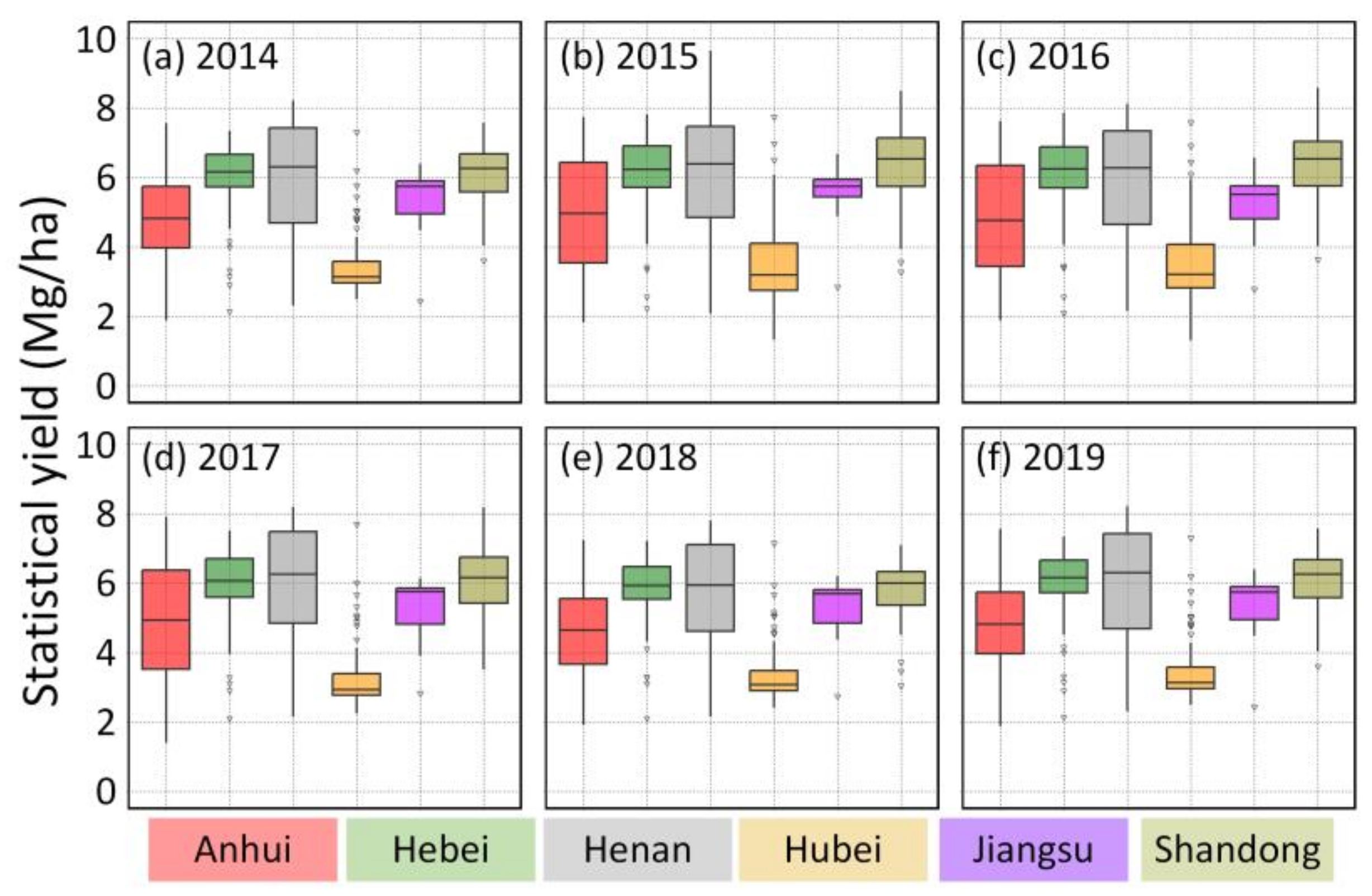
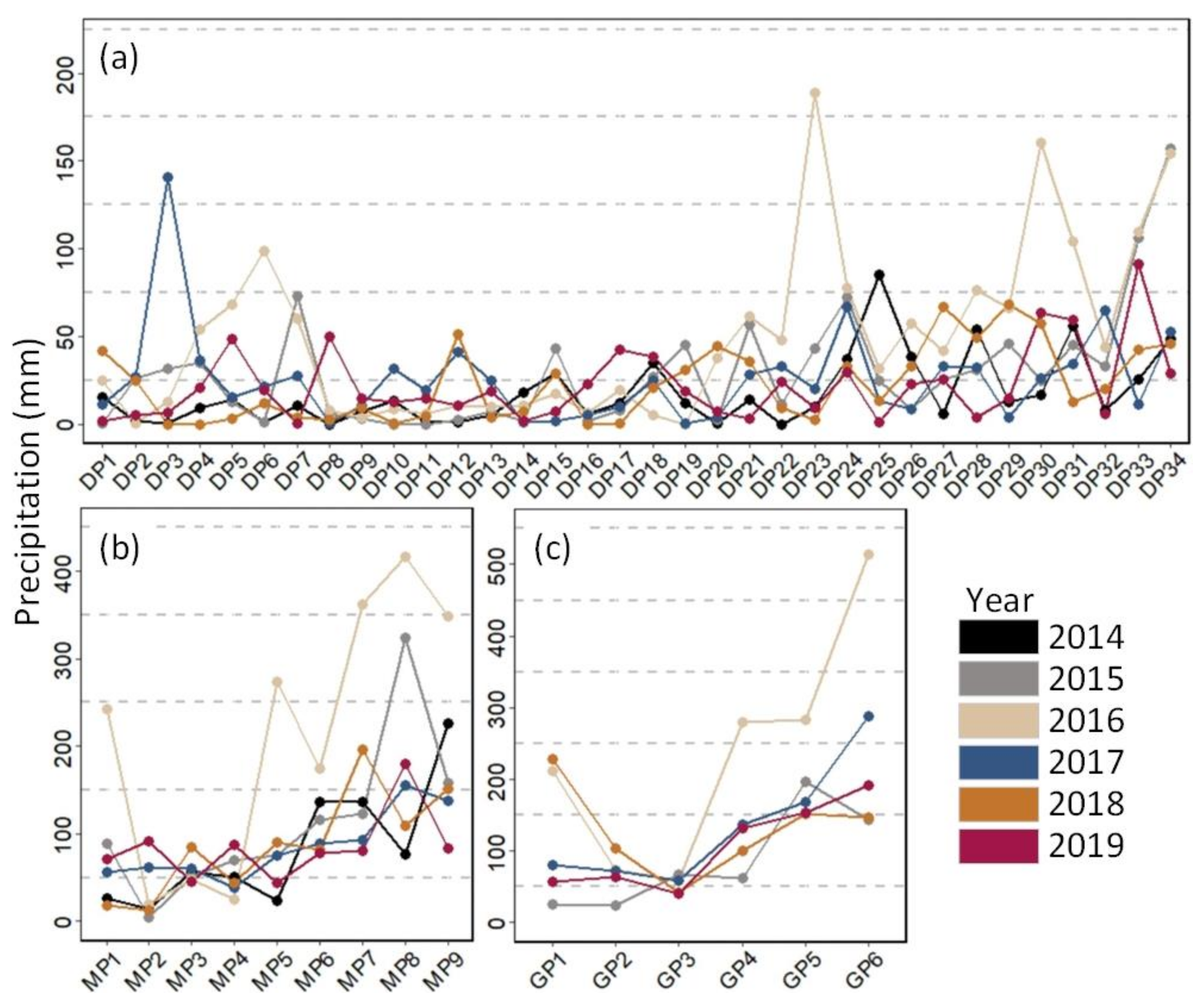
3.1. Descriptive Statistics

The box plot of the statistical yield results (Figure 3) revealed that although there were differences in the county-level statistical yield distributions among the different provinces, the yield gaps among the provinces were consistent. Henan, Hebei, and Shandong had relatively high wheat yields, all of which were above 6 Mg/ha, and Hubei Province had the lowest yield, approximately 3.6 Mg/ha. The variation in county yield was large in Anhui Province. The yield range from 2014–2019 was greater than 5 Mg/ha. In Jiangsu Province, the range of yield was small; from 2014–2019, it was 4, 3.8, 3.7, 3.3, 3.5, and 4 Mg/ha, respectively.

The feature variables used in this study all presented seasonal patterns, and the variation curves presented obvious peaks or troughs (Figures S1–S10). As the time length of the feature variables decreased, the change curve gradually smoothed (Figure 4).

For example, during the greening–rise period (GP3) of winter wheat, wheat seedlings began to grow rapidly, the leaf color changed from yellow to green, photosynthesis increased, vegetation coverage and biomass increased rapidly, and the NDVI value rose rapidly (Figure 4, red arrow). However, after the flowering stage, winter wheat began to enter the grain-filling stage, the leaves gradually aged, and the NDVI value began to decrease gradually. As the maturity stage approached, the plants gradually lost their green vegetation characteristics, the NDVI value declined rapidly, and the curve showed a significant downward trend (Figure 4, black arrow).

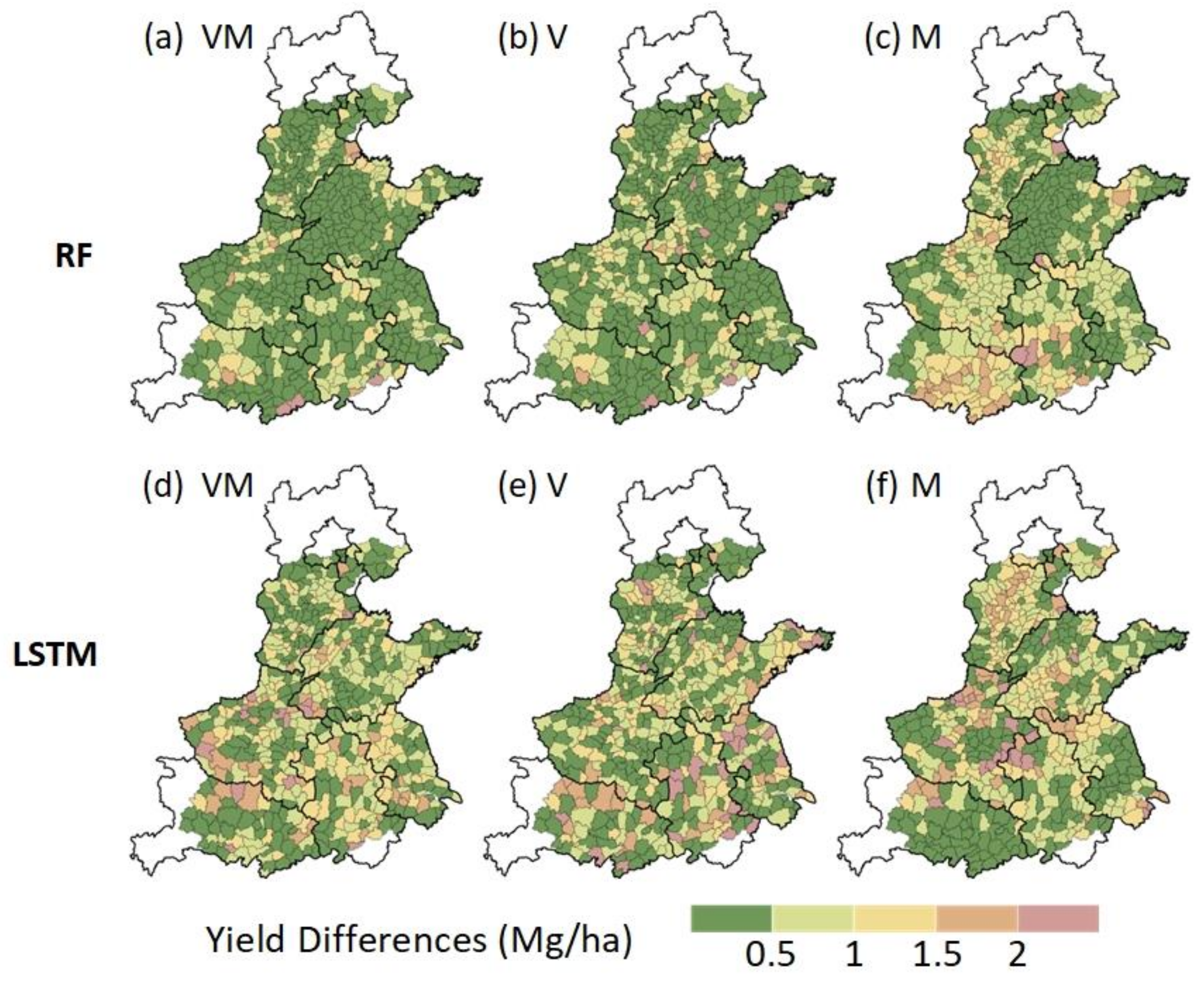
3.2. Model-Performance Evaluation

These two machine-learning methods have different model accuracies for different time-series data, and there is high consistency in the differences between provinces (

Table 6. RMSE (root mean square error) and R² (coefficient of determination) for the yield simulated by machine-learning models and the statistical yield. ML, machine-learning approaches used in this research; RF, random forest; LSTM, long short-term memory network; V, vegetation indices; M: meteorological indices; DP, composite for the 8-day period; MP, composite for the monthly period; GP, composite for the growth periods.

Province	ML	Variable
		DP-VM	DP-V	DP-M	MP-VM	MP-V	MP-M	GP-VM	GP-V	GP-M
Anhui	RF	0.79 (0.56)	0.82 (0.53)	1.04 (0.46)	0.73 (0.62)	0.75 (0.6)	0.83 (0.54)	0.74 (0.6)	0.79 (0.58)	1.3 (0.58)
	LSTM	1.06 (0.36)	1.87 (0.06)	1.17 (0.2)	0.95 (0.45)	1.15 (0.55)	1.12 (0.2)	0.83 (0.53)	1.09 (0.44)	1.05 (0.64)
Hebei	RF	0.65 (0.51)	0.66 (0.48)	0.91 (0.07)	0.6 (0.56)	0.64 (0.5)	0.87 (0.07)	0.68 (0.46)	0.63 (0.51)	1.02 (0.05)
	LSTM	1.03 (0.22)	1.09 (0.32)	1.2 (0.05)	0.72 (0.56)	0.84 (0.49)	0.99 (0.38)	0.76 (0.41)	0.71 (0.49)	1.08 (0.06)
Henan	RF	0.49 (0.88)	0.69 (0.82)	0.97 (0.66)	0.62 (0.83)	0.72 (0.75)	0.65 (0.82)	0.59 (0.85)	0.65 (0.83)	0.62 (0.81)
	LSTM	1.32 (0.22)	1.07 (0.47)	1.92 (0.17)	0.94 (0.56)	0.98 (0.55)	1.57 (0.16)	0.97 (0.58)	1.21 (0.47)	1.13 (0.4)
Hubei	RF	0.71 (0.33)	0.7 (0.35)	1.19 (0.115)	0.6 (0.41)	0.67 (0.39)	0.69 (0.43)	0.75 (0.42)	0.92 (0.25)	1.23 (0.17)
	LSTM	1.33 (0.15)	1.67 (0.02)	0.95 (0.08)	0.81 (0.28)	0.87 (0.05)	0.82 (0.08)	0.84 (0.37)	0.88 (0.21)	0.88 (0.03)
Jiangsu	RF	0.52 (0.42)	0.54 (0.38)	0.66 (0.07)	0.4 (0.66)	0.45 (0.61)	0.52 (0.47)	0.63 (0.53)	0.76 (0.15)	0.5 (0.46)
	LSTM	1.15 (0.02)	1.2 (0.15)	0.97 (0.03)	0.55 (0.51)	0.64 (0.31)	1.01 (0.16)	0.55 (0.35)	0.52 (0.38)	0.8 (0.01)
Shandong	RF	0.67 (0.32)	0.8 (0.41)	0.76 (0.15)	0.71 (0.67)	0.67 (0.6)	0.7 (0.44)	0.62 (0.61)	0.6 (0.42)	0.67 (0.21)
	LSTM	1 (0.3)	1.07 (0.1)	0.82 (0.12)	0.54 (0.46)	0.57 (0.39)	0.65 (0.16)	0.51 (0.45)	0.63 (0.38)	0.7 (0.21)

). This study focused on the following three aspects:

First, the RF accuracy was generally higher than that of the LSTM. Taking the DP-VW simulation scenario in Anhui Province as an example, the RMSE of the RF model was 0.79 Mg/ha, while the RMSE of the LSTM model was 1.06 Mg/ha; the RMSE decreased by 0.27 Mg/ha, and the R² decreased from 0.56 to 0.36. The RMSE of the RF model in other provinces was lower than that of the LSTM model, among which the RMSE of the RF model was reduced by 0.38 in Hebei Province, 0.83 Mg/ha in Henan Province, 0.62 Mg/ha in Hubei Province, 0.63 Mg/ha in Jiangsu Province, and 0.33 Mg/ha in Shandong Province. The average decrease in the six provinces was 0.5 Mg/ha.

Second, in the simulation scenarios constructed in this study, most of the model accuracies from high to low were VW, V, and W. Taking Hubei Province as an example, under the premise of the same time-series simulation data, the RMSEs of the RF models from low to high were DP-VW, DP-V, and DP-W, indicating that comprehensive vegetation indices and meteorological indices could obtain better simulation results, but there were also exceptions. For example, the RMSE of MP-V in Henan Province was greater than that of MP-W;

Third, the length of the time series exhibited different effects on the model accuracy across different provinces. As the length of the time series decreased, the accuracy of the RF model increased in Anhui Province and Shandong Province, while the accuracy of the other provinces decreased and the accuracy of the LSTM model increased. The simulation scenarios of DP-VW, MP-VW, and GP-VW in Anhui Province were taken as examples. The RMSE of the LSTM model decreased from 1.06 to 0.83.

Through error spatial mapping, we can more intuitively observe the spatial distribution characteristics and changing trends of errors in different provinces, mainly including the following two aspects:

First, the error in the RF model was obviously smaller than that of the LSTM model, and it has spatial clustering characteristics. Taking the DP-VW simulation scenario as an example, the RF error was mostly less than 0.5 Mg/ha, and the areas with small errors were concentrated in areas with relatively flat terrain, such as Western Shandong Province and Eastern Henan Province (Figure 5a), whereas the LSTM error had no obvious spatial characteristics. In addition, randomness (Figure 5d) is presented.

Second, from DP to GP, as the training feature temporal resolution changed from an 8-day composite to a growth period composite, the length of the LSTM training data decreased, the LSTM errors decreased significantly, and most regional errors were reduced to less than 1 Mg/ha. The spatial distribution of the errors exhibited spatial aggregation. The lower errors were located mainly in areas with relatively flat terrain, such as Southwest Shandong Province and Jiangsu Province. The higher errors were mainly concentrated in regions with large topographic and spatial heterogeneity, such as Hubei Province (Figure 6d and Figure 7d).

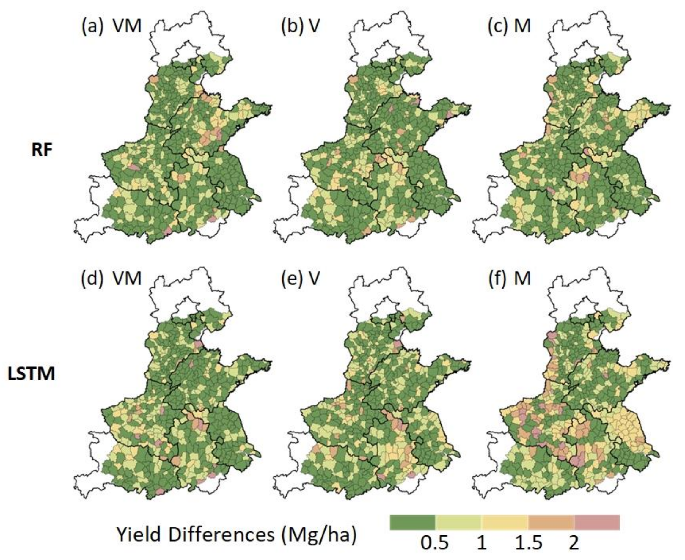
3.3. Model Performance Under Extreme Weather Conditions

Owing to the strong El Nino phenomenon in 2016, Anhui Province experienced heavy rainfall and flood disasters [33]. Therefore, the 2016 yield data of Anhui Province were used as the verification data to test the prediction accuracy of the RF and LSTM models under extreme climate conditions. All the vegetation indices and meteorological indices were selected as training features, and the training data were the data of all the other years except 2016. As seen in the line chart, from February 2016 (MP5) to June 2016, the precipitation was mostly in the key growth period of winter wheat, and the average precipitation in the province even reached more than 400 mm (Figure 8). Similarly, the RF simulation accuracy was greater than that of the LSTM model (Figure 9). Under the three time series, the RF RMSE was less than 1 Mg/ha, the R² was greater than 0.5, and the predicted yield and statistical yield had better fitting effects.

3.4. Effects of Different Period Data on Model Accuracy

In time series data modeling, the data from different periods are added to the yield prediction model, which helps to identify the key time of yield prediction according to the change in model accuracy. Taking Anhui Province as an example, when the data from October (MP1) alone were used, the RF RMSE was 1.82 Mg/ha. After the data from November (MP2) were added, the RMSE decreased to 0.90 Mg/ha (

Table 7. Results of the RMSE (root mean square error) for the yield simulated by machine-learning models and the statistical yield. ML, machine-learning approaches used in this research; RF, random forest; LSTM, long short-term memory network; MP, composite for monthly periods.

Province	ML	Monthly Periods
		MP1	MP2	MP3	MP4	MP5	MP6	MP7	MP8	MP9
Anhui	RF	1.82	0.90	0.94	0.94	0.92	0.83	0.76	0.74	0.73
	LSTM	1.37	1.02	1.22	1.50	1.54	1.07	0.83	1.05	0.95
Hebei	RF	1.36	0.74	0.79	0.79	0.78	0.74	0.64	0.62	0.60
	LSTM	0.94	0.81	0.80	0.80	0.79	0.78	0.74	0.68	0.71
Henan	RF	1.29	1.23	1.21	1.13	1.16	1.11	1.09	0.78	0.62
	LSTM	1.31	1.18	1.05	1.11	1.04	0.95	1.10	1.00	0.94
Hubei	RF	1.09	0.90	0.85	0.78	0.84	0.76	0.71	0.71	0.70
	LSTM	1.15	1.06	0.92	0.86	0.92	0.88	0.88	0.77	0.81
Jiangsu	RF	0.94	0.62	0.60	0.60	0.57	0.53	0.53	0.48	0.40
	LSTM	0.78	0.71	0.53	0.62	0.55	0.50	0.52	0.56	0.55
Shandong	RF	1.40	1.32	0.94	0.93	0.92	0.80	0.75	0.78	0.74
	LSTM	0.90	0.72	0.69	0.67	0.67	0.71	0.67	0.70	0.54

). The RF RMSE decreased from 0.99 Mg/ha to 0.59 Mg/ha after the addition of the GP6 data in Henan Province and from 0.94 Mg/ha to 0.62 Mg/ha after the addition of the GP2 data in Jiangsu Province. The LSTM RMSE decreased from 1.36 Mg/ha to 0.89 Mg/ha after adding the GP4 data in Anhui Province and from 1.2 Mg/ha to 0.85 Mg/ha after adding the GP2 data in Hebei Province (

Table 8. Results of the RMSE (root mean square error) for the yield simulated by machine-learning models and the statistical yield. ML, machine-learning approaches used in this research; RF, random forest; LSTM, long short-term memory network; GP, composite for growth periods.

Province	ML	Growth Periods
		GP1	GP2	GP3	GP4	GP5	GP6
Anhui	RF	0.92	0.84	0.83	0.77	0.76	0.74
	LSTM	1.51	1.15	1.36	0.89	0.88	0.83
Hebei	RF	0.79	0.78	0.80	0.77	0.77	0.68
	LSTM	1.20	0.85	0.79	0.74	0.77	0.76
Henan	RF	1.22	1.09	1.08	1.06	0.99	0.59
	LSTM	1.41	1.07	1.01	0.99	0.97	0.97
Hubei	RF	1.30	1.00	0.89	0.87	0.88	0.75
	LSTM	1.13	0.99	0.91	0.88	0.87	0.84
Jiangsu	RF	0.94	0.68	0.68	0.64	0.65	0.63
	LSTM	0.88	0.698	0.568	0.558	0.60	0.55
Shandong	RF	1.02	0.84	0.76	0.78	0.63	0.62
	LSTM	0.72	0.60	0.65	0.57	0.56	0.51

). Therefore, within the growing season, the prediction accuracy of the model can be improved as the data near the end of the growing season are added to the model (Table 7 and Table 8).

4. Discussion

4.1. Construction of the Time Series Prediction Model

Owing to the seasonal characteristics of crop growth and the obvious trend between the change in crop growth parameters and the change in the natural environment during different growth periods, which is in line with the basic conditions of time-series data modeling, in this study, a winter wheat prediction model was established by using three different types of time series data and two machine-learning methods, RF and LSTM. To study the effect of time-series length on yield prediction accuracy, the key time points of yield prediction are obtained.

Extracting features from the time-series data was crucial to the yield prediction model [34]. Previous studies used monthly data during the wheat growing season to construct yield prediction models [34]. However, to better reflect the change in winter wheat growth, this study used the MOD09A1 8-day composite product to calculate the vegetation index. By constructing feature variables with different time lengths, the influence of time length on model accuracy can be verified. Owing to the obvious period of winter wheat growth, this study calculated the mean value of the feature variables in each time step and aggregated the features with the county region as the basic spatial unit. However, when the time-series data did not have obvious periodic changes or seasonal patterns, it is necessary to extract the information in time series data by using the signal-enhancement method [35].

In related research on prediction modeling accuracy, the results of the yield prediction model showed that the RF model was significantly better than machine-learning models, such as multilayer perceptron and LASSO [20,36]. In the study of soil organic carbon prediction in Southern Xinjiang, China, three different sample sizes, 330, 660, and 990, have been used [37]. When the sample size of the training data was small and the features were simple, the accuracy of the RF model was not much different from that of the deep-learning model. Thus, fully exploiting the advantages of deep learning is difficult. Moreover, the RF model has the advantages of simple modeling and low operational complexity. When the sample size increases to a certain extent, deep-learning models, such as LSTM and CNN, have more significant advantages [37].

Combined with the simulation scenario constructed in this study, the dimensions of the training data in the five provinces were relatively small. Taking the simulation scenario DP as an example, the data dimensions of the feature variables of the random forest model in Anhui Province were 285 rows and 340 columns (Table 4). Therefore, when the dimensions of the feature variables were small, the results showed that in the prediction of winter wheat yield in China, the RF model was superior to the LSTM model. Because the occurrence frequency of extreme climates is low and often sudden, and the climatic conditions in the time series are quite different from those in the previous period, the LSTM model may not be able to simulate accurately when it encounters the type or intensity of extreme climate that has never appeared in historical data. Therefore, it was necessary to synthesize model application scenarios, maintenance costs, and model interpretability and use appropriate models rather than more complex models to obtain accurate results.

In addition, because the collected data cannot cover all extreme climate conditions, as well as other factors, such as pests and diseases, the selected feature variables of the model have limitations, and the prediction model should be constantly updated to adapt to new situations [34]. However, meteorological, soil, and, especially, vegetation indices should be considered as much as possible in modeling. On the basis of this study and previous studies, the yield prediction model based on meteorological, soil, and vegetation indices has the highest prediction accuracy [36,38].

4.2. Optimal Yield Prediction Time

Studying the optimal prediction time of the yield prediction model can guide the time and frequency of data collection, reduce the cost of data collection and the complexity of model calculation, and improve the accuracy of yield prediction. For example, by analyzing the time sensitivity of the crop model and then obtaining satellite image data during the key period, the process parameters of the crop model, including the leaf-area index and dry-matter content, can be inverted to improve the yield prediction accuracy of the crop model [4,39,40]. Among them, the single-factor analysis method has been widely used because of its simple operation; that is, the data of different periods are used for yield prediction. When the data of a specific excluded time range had a great impact on the model prediction accuracy, this time range was the key period of yield prediction [21,41,42].

Crop growth includes two stages: vegetative growth and reproductive growth. Many previous studies have shown that the yield prediction model established in the reproductive growth stage, including the wheat-heading stage to the grain-filling stage and the maize stub stage to the early grain-filling stage, has high prediction accuracy [14,34,38,39]. In this study, the single-factor analysis method was used to obtain the key time points predicted by each province through the changes in the RMSE and R², which only changed the time variable while other feature variables remained unchanged. Similar to the results of previous studies, from the bar diagram distribution, the more data used, the higher the accuracy of the model (Figure 10 and Figure 11) [22]. However, there were obvious inflection points in some provinces, such as November in Anhui Province, May in Henan Province (Figure 8), and the flowering period (GP5) in Henan Province (Figure 11a).

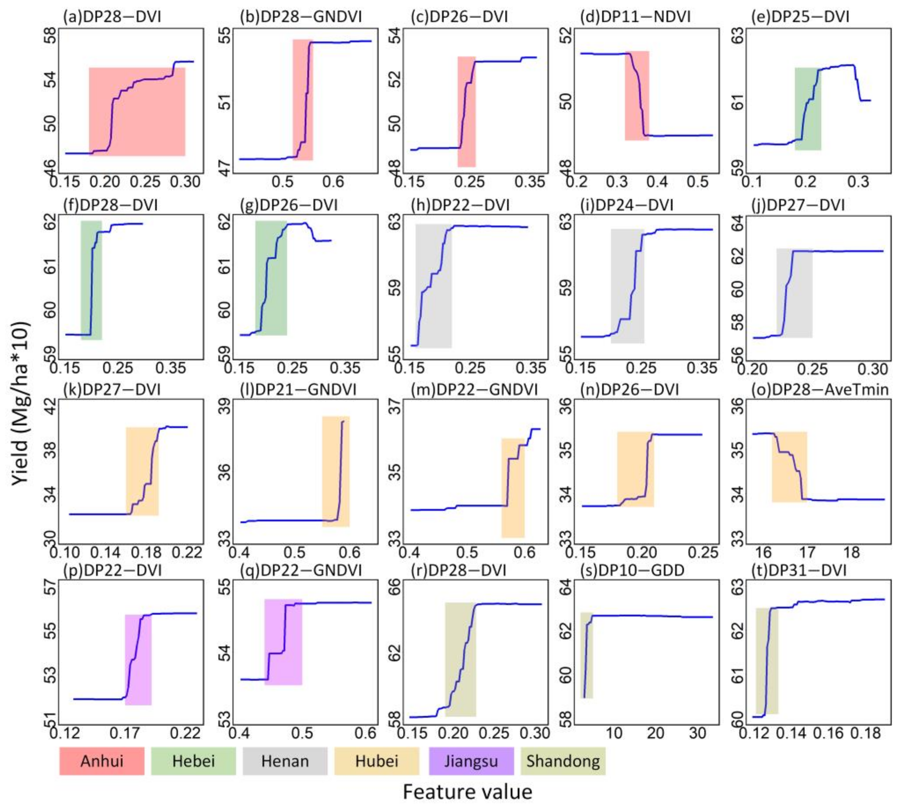
4.3. Nonlinear Relationship Between Feature Variables and Yield

Quantifying the degree of influence of feature variables on yield variation could improve the interpretability of machine-learning models and help to identify yield-limiting factors. The commonly used methods include the correlation test, SHAP analysis, and ridge regression [6,10,12,23,34,43,44]. Since RF was insensitive to the collinearity of multiple feature variables, using RF to conduct feature importance tests based on tree models can intuitively reveal the nonlinear relationships between feature variables and target variables (Figure 10, Figure 11 and Figure 12). As shown in the figure, the vegetation indices and meteorological indices used in this study appear in the feature importance maps of different time-series data, but the following rules exist. First, the vegetation indices can directly reflect the vegetation coverage and growth status, there was a positive correlation between the vegetation index and the formation of biomass [36,38]. For example, in our research, when the DVI value rises from 0.2 to 0.3, the yield rises from about 4.7 Mg/ha to 5.5 Mg/ha (Figure 10a, red box). However, when the value of the vegetation index exceeds a threshold, the yield no longer changes. For example, when DVI exceeds 0.25, the yield has been stable at about 6.5 Mg/ha (Figure 11g, grey box). This phenomenon existed in all three simulation scenarios (Figure 10, Figure 11 and Figure 12). Secondly, since the single GP covers 42 days, the time resolution of feature variables was reduced, and meteorological indices have cumulative effects on crops, there was a non-linear relationship between temperature, precipitation, and yield in different growth periods of crops (Figure 12).

The concept of GDD mainly refers to the accumulation of heat within a suitable growth-temperature range. In the vegetative growth stage of winter wheat, sufficient heat accumulation is conducive to the growth of vegetative organs such as leaves and stems, effectively improves photosynthesis efficiency, promotes dry-matter accumulation, and provides a material basis for the formation and development of seeds in the reproductive growth stage, which is crucial for the final yield. Therefore, for the northern regions with low temperatures, including Shandong and Henan, the higher the GDD was, the higher the yield was (Figure 10, Figure 11 and Figure 12n,ad). However, under conditions of sufficient GDD, the occasional extremely high temperature accelerated plant senescence, reduced the duration of grain-filling, and led to a decrease in yield, which may have been caused by the grain-filling and maturity stage (GP6) in Shandong Province. The main reason for the decline in production occurred when the number of GDD exceeded 1060 (Figure 12ad). This phenomenon also occurs in May (MP8) and during the grain-ripening period (GP6) of winter wheat, when the KDD exceeds 75 and the yield decreases (Figure 11s). When the GDD reaches a certain value, the output may no longer increase with increasing GDD; that is, a saturation phenomenon occurs. This occurred because crop yields are also limited by other factors, such as light duration, soil fertility, and water availability [38]. At this point, the number of GDD was no longer the only factor limiting yield, and other environmental and physiological factors began to play a dominant role (Figure 11q).

There was an obvious nonlinear relationship between the vegetation indices and yield at different growth stages, and small changes in the vegetation indices may lead to large changes in yield. In the early growth stage of winter wheat, the yield gradually increased with increasing DVI. Taking Hubei Province as an example, the DVI increased from 0.16 to 0.17, and the yield increased from 3.4 Mg/ha to 3.58 Mg/ha (Figure 11n and Figure 12s,v). However, in the later growth stage of winter wheat, such as the flowering stage (GP5), the yield increased gradually. When the DVI was greater than 0.24, the yield changes tended to be stable (Figure 10a,f–k, Figure 11b,c,f,h,k,q and Figure 12a,h,o,s,y,ae), and the yield changes were large. The DVI of Anhui Province increased from 0.22 to 0.24. The yield increased from 4.1 Mg/ha to 6.5 Mg/ha (Figure 12a), the DVI in Henan Province increased from 0.2 to 0.28, and the yield increased from 4.5 Mg/ha to 6.9 Mg/ha (Figure 12m). The GNDVI, DVI, and yield exhibited similar trends (Figure 10b,l,m,q, Figure 11d,l,p and Figure 12f).

Consistent with previous studies, there was a strong relationship between the minimum temperature and winter wheat yield during the growing season [12,38]. In this study, AveTmin was significantly negatively correlated with yield (Figure 10o, Figure 11a,e,r and Figure 12c,g,l,x,z). Taking Hebei Province as an example, when the AveTmin of the tiller overwintering stage (GP2) increased from −5 °C to −4 °C, the yield decreased from 6.15 Mg/ha to 6 Mg/ha, possibly because the increase in temperature accelerated the growth process of winter wheat and led to a reduction in the number of grains per spike; that is, the winter wheat grew too fast. This led to a negative correlation between the vegetation indices and yield (Figure 10d, Figure 11v,y and Figure 12e,k) [38]. However, most AveTmax values were positively correlated with yield (Figure 12p,q,aa), and maintaining a suitable temperature range of 12–16 °C during the join–booting stage (GP4) played an important role in ensuring the number of grains per spike (Figure 12aa). EP is very important for winter wheat filling. However, excessive EP leads to impaired respiration of crop roots, which are unable to absorb water and nutrients, which inhibits aboveground growth and ultimately leads to decreased yield. This may be the main reason for the negative correlation between EP and yield at the joint-booting stage (GP4) and heading stage (GP5) in Anhui and Hubei Provinces (Figure 12d,t,u).

4.4. Limitations

The generalization ability of machine-learning models is limited by the training data; if the new data have similar underlying patterns to the training data, the model has the potential to make predictions on the basis of what it has learned. However, when the distribution of new data is very different from that of the training data, such as when the extremely abnormal climate is completely different from the climate conditions in the training data, the model makes predictions on the basis of the previously learned rules, and the results may be inaccurate. To improve the generalizability of the model at different spatial scales, in addition to the natural environment, the factors influencing crop growth are affected by agricultural machinery, fertilizer, the planting system, and other policy and economic factors. Owing to the difficulty in obtaining time-series data, this study did not consider them. In addition, through the collection of plot-level yield data, comprehensive meteorological soil data, more accurate spectral data collected by drones, and agricultural factor input data, the realization of smaller-scale yield predictions at the county level, farm level, and plot level is the main direction for the future application of precision agriculture [5]. Finally, this study uses only the data-driven approach of the spatial environment to build a model without considering the mechanism relationship between crops and the environment, regional heterogeneity, continuity, and spatial autocorrelation of yield, as well as coupling the process mechanism of the crop growth model with the machine learning model [14,36]. Adding yield spatial-structure features to the construction of feature variables is the main direction of further research.

5. Conclusions

By studying the influence of the time length of environmental data on the accuracy of crop yield prediction, we can reduce the redundancy of modeling data and improve the representation of feature extraction so as to ensure the efficiency and accuracy of crop yield simulation. Vegetation indices, such as DVI, were important indicators that directly reflected yield changes. Using vegetation indices and meteorological indices together can achieve high prediction accuracy, and the average RMSE of RF was 0.5 Mg/ha lower than LSTM model in all simulation scenarios, which has a high modeling accuracy. As the length of the time series gradually shortens from DP to GP, the RMSE of both RF and LSTM models were lower than 1 Mg/ha. Using low time-resolution features can improve yield prediction accuracy, and using the data close to the later stage of crop growth can improve the model’s confidence. This study determined the appropriate time lengths of feature variables and the key time points for yield prediction, confirmed the feasibility of using environmental data with low temporal resolution, and provided a reference for data selection in crop yield prediction using machine learning.

References

1. Xu, H.; Zhang, X.; Ye, Z.; Jiang, L.; Qiu, X.; Tian, Y.; Zhu, Y.; Cao, W. Machine learning approaches can reduce environmental data requirements for regional yield potential simulation. Eur. J. Agron. 2021, 129, 126335. [Google Scholar] [CrossRef]
2. Zhang, X.; Xu, H.; Jiang, L.; Zhao, J.; Zuo, W.; Qiu, X.; Tian, Y.; Cao, W.; Zhu, Y. Selection of Appropriate Spatial Resolution for the Meteorological Data for Regional Winter Wheat Potential Productivity Simulation in China Based on WheatGrow Model. Agronomy 2018, 8, 198. [Google Scholar] [CrossRef]
3. Klompenburg, T.V.; Kassahun, A.; Catal, C. Crop yield prediction using machine learning: A systematic literature review. Comput. Electron. Agric. 2020, 177, 105709. [Google Scholar] [CrossRef]
4. Zare, H.; Weber, T.K.; Ingwersen, J.; Nowak, W.; Gayler, S.; Streck, T. Within-season crop yield prediction by a multi-model ensemble with integrated data assimilation. Field Crops Res. 2024, 308, 109293. [Google Scholar] [CrossRef]
5. Cheng, Z.; Gu, X.; Zhou, Z.; Zhang, Y.; Yin, H.; Li, W.; Chang, T.; Du, Y. Enhancing in-season yield forecast accuracy for film-mulched wheat: A hybrid approach coupling crop model and UAV remote-sensing data by ensemble learning technique. Eur. J. Agron. 2024, 156, 127174. [Google Scholar] [CrossRef]
6. Sharafi, S.; Nahvinia, M. Sustainability insights: Enhancing rainfed wheat and barley yield prediction in arid regions. Agric. Water Manag. 2024, 299, 108857. [Google Scholar] [CrossRef]
7. Perich, G.; Turkoglu, M.; Graf, L.; Wegner, J.; Aasen, H.; Walter, A.; Liebisch, F. Pixel-based yield mapping and prediction from Sentinel-2 using spectral indices and neural networks. Field Crops Res. 2023, 292, 108824. [Google Scholar] [CrossRef]
8. Tanabe, R.; Matsui, T.; Tanaka, T. Winter wheat yield prediction using convolutional neural networks and UAV-based multispectral imagery. Field Crops Res. 2023, 291, 108786. [Google Scholar] [CrossRef]
9. Arslan, N.; Sekertekin, A. Application of Long Short-Term Memory neural network model for the reconstruction of MODIS Land Surface Temperature images. J. Atmos. Solar-Terr. Phys. 2019, 194, 105100. [Google Scholar] [CrossRef]
10. Clercq, D.; Mahdi, A. Feasibility of machine learning-based rice yield prediction in India at the district level using climate reanalysis and remote sensing data. Agric. Syst. 2024, 220, 104099. [Google Scholar] [CrossRef]
11. Yin, X.; Peng, J.; Huang, S.; Leng, G. Aggravation of global maize yield loss risk under various hot and dry scenarios using multiple types of prediction approaches. Int. J. Clim. 2024, 44, 4. [Google Scholar] [CrossRef]
12. Silva, J.; Heerwaarden, J.; Reidsma, P.; Laborte, A.; Tesfaye, K.; Ittersum, M. Big data, small explanatory and predictive power: Lessons from random forest modeling of on-farm yield variability and implications for data-driven agronomy. Field Crops Res. 2023, 302, 109063. [Google Scholar] [CrossRef] [PubMed]
13. Apolo-Apolo, O.; Martínez-Guanter, J.; Egea, G.; Raja, P.; Perez-Ruiz, M. Deep learning techniques for estimation of the yield and size of citrus fruits using a UAV. Eur. J. Agron. 2020, 115, 126030. [Google Scholar] [CrossRef]
14. Li, J.; Li, G.; Wang, L.; Li, D.; Li, H.; Gao, C.; Zhuang, M.; Zhuang, J.; Zhou, H.; Xu, S.; et al. Predicting maize yield in Northeast China by a hybrid approach combining biophysical modelling and machine learning. Field Crop. Res. 2023, 302, 109102. [Google Scholar] [CrossRef]
15. Khaki, S.; Pham, H.; Wang, L. Simultaneous corn and soybean yield prediction from remote sensing data using deep transfer learning. Sci. Rep. 2021, 11, 11132. [Google Scholar] [CrossRef]
16. Lobell, D. The use of satellite data for crop yield gap analysis. Field Crops Res. 2013, 143, 56–64. [Google Scholar] [CrossRef]
17. Richetti, J.; Lawes, R.; Whan, A.; Gaydon, D.; Thorburn, P. How well does APSIM NextGen simulate wheat yields across Australia using gridded input data? Validating Continental-Scale Crop Model Simulations. Eur. J. Agron. 2024, 158, 127212. [Google Scholar] [CrossRef]
18. Li, S.; Jiang, S.; Song, N.; Han, Y.; Wang, J. Two-step fusion framework for generating 10 m resolution soil moisture with high accuracy in the cotton fields of southern Xinjiang. Ind. Crops Prod. 2025, 226, 120582. [Google Scholar] [CrossRef]
19. Wang, M.; Ciais, P.; Frappart, F.; Tao, S.; Fan, L.; Sun, R.; Li, X.; Liu, X.; Wang, H.; Wigneron, J.P. A novel AMSR2 retrieval algorithm for global C-band vegetation optical depth and soil moisture (AMSR2 IB): Parameters’ calibration, evaluation and inter-comparison. Remote Sens. Environ. 2024, 313, 114370. [Google Scholar] [CrossRef]
20. Zhou, J.; Jia, L.; Menenti, M. Reconstruction of global MODIS NDVI time series: Performance of Harmonic ANalysis of Time Series (HANTS). Remote Sens. Environ. 2015, 163, 217–228. [Google Scholar] [CrossRef]
21. Tan, Z.; Yue, P.; Di, L.; Tang, J. Deriving High Spatiotemporal Remote Sensing Images Using Deep Convolutional Network. Remote Sens. 2018, 10, 1066. [Google Scholar] [CrossRef]
22. Jiang, H.; Hu, H.; Zhong, R.; Xu, J.; Xu, J.; Huang, J.; Wang, S.; Ying, Y.; Lin, T. A deep learning approach to conflating heterogeneous geospatial data for corn yield estimation: A case study of the US Corn Belt at the county level. Glob. Change Biol. 2020, 26, 1754–1766. [Google Scholar] [CrossRef] [PubMed]
23. Ashapure, A.; Jung, J.; Chang, A.; Oh, S.; Yeom, J.; Maeda, M.; Maeda, A.; Dube, N.; Landivar, J.; Hague, S.; et al. Developing a machine learning based cotton yield estimation framework using multi-temporal UAS data. ISPRS J. Photogramm. Remote Sens. 2020, 169, 180–194. [Google Scholar] [CrossRef]
24. Yang, G.; Yu, W.; Yao, X.; Zheng, H.; Cao, Q.; Zhu, Y.; Cao, W.; Cheng, T. AGTOC: A novel approach to winter wheat mapping by automatic generation of training samples and one-class classification on Google Earth. Int. J. Appl. Earth Obs. Geoinf. 2021, 102, 102446. [Google Scholar] [CrossRef]
25. Döll, P.; Siebert, S. Global modeling of irrigation water requirements. Water Resour. Res. 2002, 38, 8-1–8-10. [Google Scholar] [CrossRef]
26. Martin, S. CROPWAT: A Computer Program for Irrigation Planning and Management. FAO Irrig. Drain. Pap. 1992, 46. [Google Scholar]
27. Grogan, S.; Anderson, J.; Baenziger, P.; Frels, K.; Guttieri, M.; Haley, S.; Kim, K.; Liu, S.; McMaster, G.; Newell, M.; et al. Phenotypic Plasticity of Winter Wheat Heading Date and Grain Yield across the US Great Plains. Crop Sci. 2016, 56, 2223–2236. [Google Scholar] [CrossRef]
28. Wang, Z.; Wang, M.; Yin, X.; Zhang, H.; Chu, Q.; Wen, X.; Chen, F. Spatiotemporal change characteristics of heat and rainfall during the growth period of winter wheat in North China Plain from 1961 to 2010. J. China Agric. Univ. 2015, 20, 16–23. [Google Scholar] [CrossRef]
29. He, X.; Luo, H.; Qiao, M.; Tian, Z.; Zhou, G. Yield estimation of winter wheat in China based on CNN-RNN network. TCSAE 2021, 37, 124–132. [Google Scholar] [CrossRef]
30. Breiman, L. Random forests. Mach. Learn. 2001, 45, 5–32. [Google Scholar] [CrossRef]
31. Gers, F.; Schmidhuber, J.; Cummins, F. Learning to Forget: Continual Prediction with LSTM. Neural Comput. 2000, 12, 2451–2471. [Google Scholar] [CrossRef] [PubMed]
32. Hochreiter, S.; Schmidhuber, J. Long Short-Term Memory. Neural Comput. 1997, 9, 1735–1780. [Google Scholar] [CrossRef] [PubMed]
33. Liu, S.; Zheng, Y.; Feng, L.; Chen, J.; Lakshmi, V.; Shi, H. Are only foods with large discharges threatening? Flood characteristics evolution in the Yangtze River Basin. Geosci. Lett. 2021, 8, 32. [Google Scholar] [CrossRef]
34. Júnior, R.; Olivier, L.; Wallach, D.; Mullens, E.; Fraisse, C.; Asseng, S. A simple procedure for a national wheat yield forecast. Eur. J. Agron. 2023, 148, 126868. [Google Scholar] [CrossRef]
35. Fan, G.; Yu, P.; Wang, Q.; Dong, Y. Short-term motion prediction of a semi-submersible by combining LSTM neural network and different signal decomposition methods. Ocean Eng. 2023, 267, 113266. [Google Scholar] [CrossRef]
36. Maseko, S.; Laan, M.; Tesfamariam, E.; Delport, M.; Otterman, H. Evaluating machine learning models and identifying key factors influencing spatial maize yield predictions in data intensive farm management. Eur. J. Agron. 2024, 157, 127193. [Google Scholar] [CrossRef]
37. Wang, Y.; Chen, S.; Hong, Y.; Hu, B.; Peng, J.; Shi, Z. A comparison of multiple deep learning methods for predicting soil organic carbon in Southern Xinjiang, China. Comput. Electron. Agric. 2023, 212, 108067. [Google Scholar] [CrossRef]
38. Jahromi, M.; Zand-Parsa, S.; Razzaghi, F.; Jamshidi, S.; Didari, S.; Doosthosseini, A.; Pourghasemi, H. Developing machine learning models for wheat yield prediction using ground-based data, satellite-based actual evapotranspiration and vegetation indices. Eur. J. Agron. 2023, 146, 126820. [Google Scholar] [CrossRef]
39. Guo, Y.; Hao, F.; Zhang, X.; He, Y.; Fu, Y. Improving maize yield estimation by assimilating UAV-based LAI into WOFOST model. Field Crops Res. 2024, 315, 109477. [Google Scholar] [CrossRef]
40. Chen, C.; Cao, G.; Li, Y.; Liu, D.; Ma, B.; Zhang, J.; Li, L.; Hu, J. Research on Monitoring Methods for the Appropriate Rice Harvest Period Based on Multispectral Remote Sensing. Discret. Dyn. Nat. Soc. 2022, 2022, 1519667. [Google Scholar] [CrossRef]
41. Zare, H.; Viswanathan, M.; Weber, T.; Ingwersen, J.; Nowak, W.; Gayler, S.; Streck, T. Improving winter wheat yield prediction by accounting for weather and model parameter uncertainty while assimilating LAI and updating weather data within a crop model. Eur. J. Agron. 2024, 156, 127149. [Google Scholar] [CrossRef]
42. Gevrey, M.; Dimopoulos, I.; Lek, S. Review and comparison of methods to study the contribution of variables in artificial neural network models. Ecol. Model. 2003, 160, 249–264. [Google Scholar] [CrossRef]
43. Hajjarpoor, A.; Soltani, A.; Zeinali, E.; Kashiri, H.; Aynehband, A.; Vadez, V. Using boundary line analysis to assess the on-farm crop yield gap of wheat. Field Crops Res. 2018, 225, 64–73. [Google Scholar] [CrossRef]
44. Bonneu, F.; Makowski, D.; Joly, J.; Allard, D. Machine learning based on functional principal component analysis to quantify the effects of the main drivers of wheat yields. Eur. J. Agron. 2024, 159, 127254. [Google Scholar] [CrossRef]
Figure 1. Spatial location (a) and DEM (digital elevation model) (b) of the study area, including Hebei (I), Shandong (II), Henan (III), Anhui (IV), Jiangsu (V), and Hubei (VI).
Agronomy 15 01114 g001
Figure 2. Technology workflow. NDVI, normalized difference vegetation index; DVI, difference vegetation index; RVI, relative vegetation index; GNDVI, Green normalized difference vegetation index; EP, effective precipitation; CP, cumulative precipitation; GDD, growing degree days; KDD, killing degree days; AveTmax, average maximum temperature; AveTmin, average minimum temperature. DP-VM, the time length of the feature variable was DP, including the vegetation indices and meteorological indices, and the other simulation scenarios were similar.
Agronomy 15 01114 g002
Figure 3. Box plot of the statistical yield. The upper line of the box is the maximum yield, the middle line is the median yield, the lower line is the minimum yield, and the black triangle denotes an outlier.
Agronomy 15 01114 g003
Figure 4. NDVI (normalized difference vegetation index) time-series curve. (af) DP, composite for the 8-day period; (gl) MP, composite for the monthly period; (mr) GP, composite for the growth periods.
Agronomy 15 01114 g004
Figure 5. Spatial distributions of the yield difference for the DP composite (composite for an 8-day period), RF, random forest; LSTM, long short-term memory network; V, vegetation indices; M: meteorological indices.
Agronomy 15 01114 g005
Figure 6. Spatial distributions of the yield difference for the MP composite (composite for a monthly period), RF, random forest; LSTM, long short-term memory network; V, vegetation indices; M: meteorological indices.
Agronomy 15 01114 g006
Figure 7. Spatial distributions of the yield difference for the GP composite (composite for the growth period), RF, and random forest; LSTM, long short-term memory network; V, vegetation indices; M, meteorological indices.
Agronomy 15 01114 g007
Figure 8. Precipitation line chart of Anhui in 2016. (a) DP, composite for 8-day periods; (b) MP, composite for monthly periods; (c) GP, composite for growth periods.
Agronomy 15 01114 g008
Figure 9. VI and MI were used as feature variables to establish a fitting line for the prediction model of winter wheat yield in Anhui Province in 2016. RMSE, root mean squared error; R2, coefficient of determination; RF, random forest; LSTM, long short-term memory network; DP, composite for 8-day periods, red points; MP, composite for monthly periods, green points; GP, composite for growth periods, blue points.
Agronomy 15 01114 g009
Figure 10. Partial dependence plots of the DP composite (composite for the 8-day period) simulation scenario with feature variables VI (vegetation indices) and MI (meteorological indices).
Agronomy 15 01114 g010
Figure 11. Partial-dependence plots of the MP composite (composite for the monthly period) simulation scenario with feature variables VI (vegetation indices) and MI (meteorological indices).
Agronomy 15 01114 g011
Figure 12. Partial-dependence plots of the GP composite (composite for the growth period) simulation scenario with feature variables VI (vegetation indices) and MI (meteorological indices).
Agronomy 15 01114 g012