DSW-YOLO-Based Green Pepper Detection Method Under Complex Environments

Abstract

In this paper, a lightweight detection model DSW-YOLO based on improved YOLOv10n is proposed. After comparing mainstream lightweight models (YOLOv5n, YOLOv6n, YOLOv8n, YOLOv9t and YOLOv10n), YOLOv10n with the best performance was selected as the baseline. The DWRR block was then designed and integrated with the C2f module to form C2f-DWRR, replacing the original C2f blocks in the backbone. Consequently, the model’s P, R, mAP50, and mAP50-95 increased by 2.3%, 2.1%, 1.8%, and 3.4%, respectively, while the parameter count dropped by 0.16 M and the model size was reduced by 0.25 MB. A SimAM parameter-free attention mechanism was added to the last layer of the backbone, boosting P, R, mAP50, and mAP50-95 to 90.6%, 84.0%, 91.8%, and 68.5%, and reducing average detection time to 1.1 ms. The CIOU function was replaced with WIOUv3 to accelerate convergence, decrease loss, and significantly enhance detection performance. Experimental results show that on a custom green pepper dataset, DSW-YOLO outperformed the baseline by achieving gains of 2.9%, 2.7%, 2.2%, and 3.4% in P, R, mAP50, and mAP50-95, reducing parameters by 1.6 M, cutting inference time by 0.7 ms, and shrinking the model size to 5.31 MB. DSW-YOLO efficiently and accurately detects green peppers in complex field conditions, significantly improving detection accuracy while remaining lightweight, and provides theoretical and technical support for designing and optimizing pepper-picking robot vision systems.

1. Introduction

Chili peppers play a significant role in rural revitalization in China [1,2], and green peppers, as a high-yield crop, find wide-ranging applications [3,4,5]. Modern agriculture is moving toward automation and mechanization, fueling demand for intelligent devices [6]. However, traditional harvesting methods often suffer from low efficiency, high costs, and fruit damage, severely constraining the green pepper industry. Therefore, promoting the intelligent development of green peppers carries substantial importance.

Advances in modern technology have made computer vision a non-contact, low-cost approach to target detection. Traditional green pepper detection methods are easily affected by occlusion, noise, and illumination changes [7,8,9], leading to low accuracy, poor robustness, and low efficiency, which hinder automatic green pepper fruit detection in complex environments. In recent years, the rapid development of artificial intelligence and deep learning especially the extensive application of convolutional neural networks (CNN) in object detection has led to significant improvements in detection technology, yielding notable progress in agricultural applications [10,11]. Based on specific processing flows, CNNs are classified as two-stage detectors or one-stage detectors. Two-stage detection models, represented by the R-CNN series [12], are widely used in agriculture. Zhang et al. [13] proposed a more precise approach for detecting and segmenting Sichuan pepper clusters on the original Mask R-CNN framework, achieving detection and segmentation accuracies of 84.0% and 77.2%, respectively. Cai et al. [14] introduced a novel Faster R-CNN algorithm for canopy recognition and canopy width extraction in high-density loblolly pine stands, demonstrating high accuracy rates of 95.26% and 95% with an improved FPN_ResNet101 model. Deng et al. [15] employed an enhanced Faster R-CNN architecture for accurate identification of sea rice panicles, using ROI align for feature aggregation and reaching a detection accuracy of up to 94.9%. Shen et al. [16] proposed a grape cluster detection and segmentation algorithm based on an enhanced Mask R-CNN, which integrates a ResNet50-FPN-ED backbone with Efficient Channel Attention (ECA) and Dense Upsampling Convolution (DUC) for multi-scale feature refinement, achieving an Average Precision (AP) of 60.1% in detection and 59.5% in segmentation under complex vineyard environments with occlusion and overlapping clusters. Although the R-CNN series offers high accuracy, its large computational complexity and substantial model size limit applications in real-time and lightweight scenarios. In contrast, single-stage detectors significantly increase detection speed and adaptability by modeling object detection as a regression problem [17], making them suitable for real-time, lightweight scenarios. Among these, the YOLO series has been widely adopted in agricultural object detection due to its rapid, efficient, and lightweight characteristics. Li et al. [18] proposed the GLS-YOLO detection model based on YOLOv8 and GhostNetV2, integrating a C2f-LC module to reduce parameters and enhance feature representation, achieving a mean average precision at IoU = 0.5(mAP50) of 90.55% on the test set. Wang et al. [19] optimized YOLOv8 for rapeseed flower recognition and counting under natural conditions, with the improved GhP2-YOLO model surpassing 95% in AP. Meanwhile, the YOLO series has also been applied to green pepper fruit detection thanks to its real-time performance, high accuracy, lightweight design, and scalability. Nan Yulong et al. [20] built a fast, accurate green pepper detection system for field environments on YOLOv5l, reaching 81.4% mAP50 at 70.9 frames per second. Li et al. [21] presented a green pepper detection algorithm based on Yolov4_tiny, achieving 96.91% precision (P) and 93.85% recall (R) by incorporating attention mechanisms and multi-scale prediction to address occlusions and small targets. Although these methods optimize the model and feature extraction, real-time detection is still challenging in dealing with complex scenes such as similar colors, morphological changes, overlapping occlusion and illumination changes. Moreover, current green pepper detection models (23.4 MB [20], 30.9 MB [21]) still leave room for further optimization toward lightweight field deployment.

Current applications of automatic green pepper picking are constrained by real-time detection capabilities and model compactness. To address these issues, an improved YOLOv10n lightweight detection algorithm is introduced to deliver a high-efficiency, precise fruit recognition model for green pepper picking robots. The main contributions include the following:

• A green pepper detection dataset was constructed, covering various fruit sizes, counts, light intensities, occlusion types, and shooting angles.
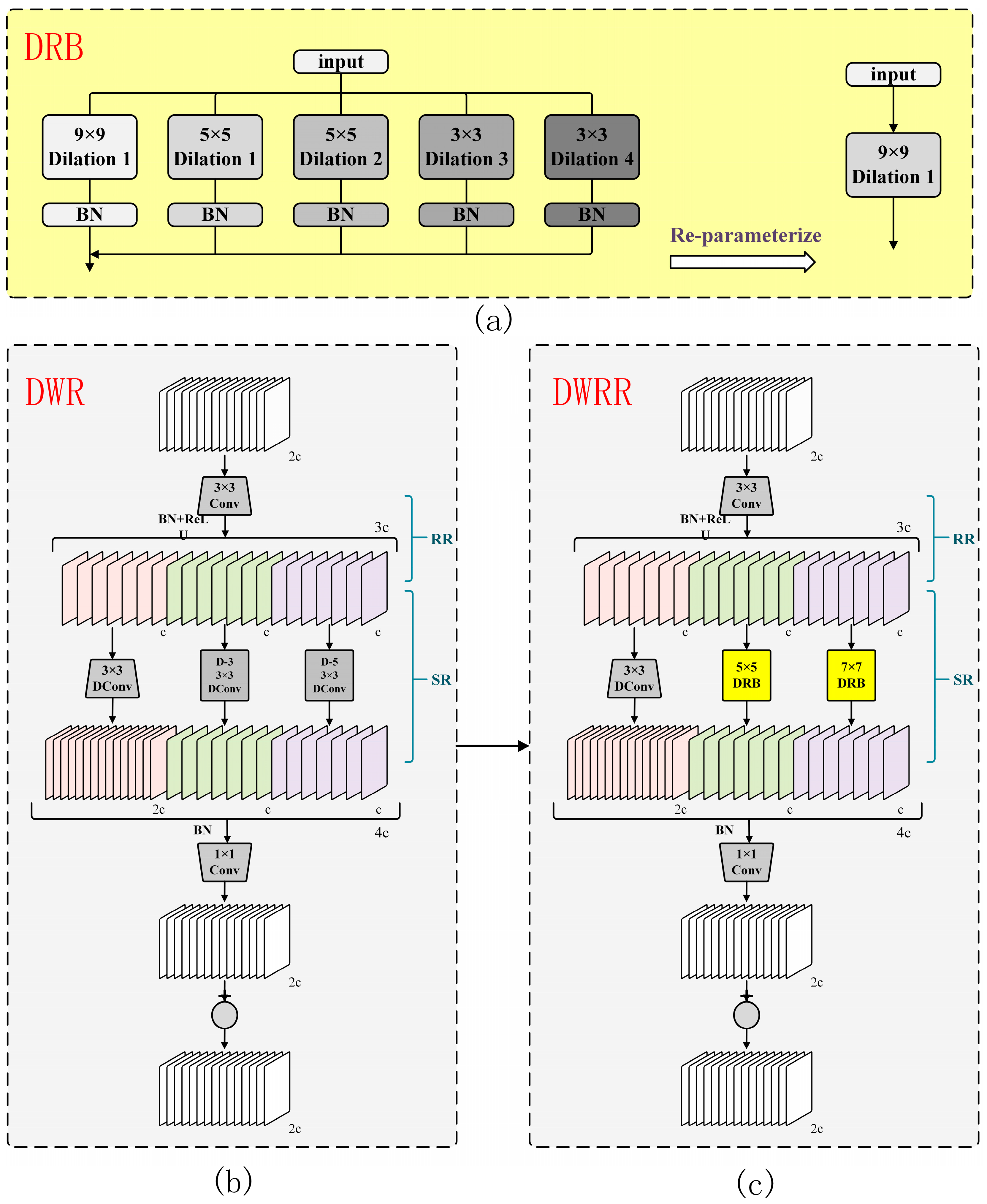
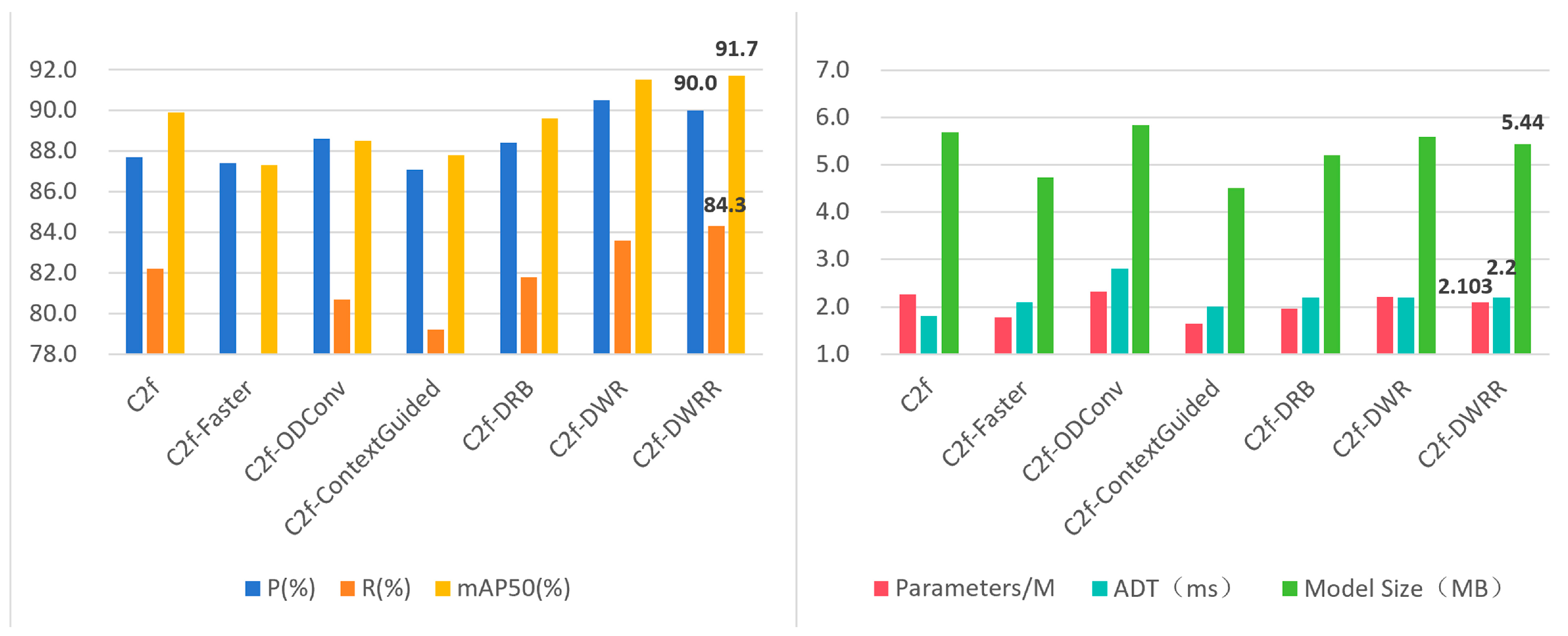
• A lightweight C2f-Dilation-wise Residual-Reparam (C2f-DWRR) module was proposed. The dilated convolution in the Dilation-wise Residual (DWR) module was replaced with a Dilated Reparam Block (DRB) module and integrated into the C2f module through class inheritance, thereby replacing the original Bottleneck structure. Substituting the 6th and 8th layers of the YOLOv10 backbone with C2f-DWRR significantly improved P and R while reducing model size and parameters, thus achieving lightweight goals.
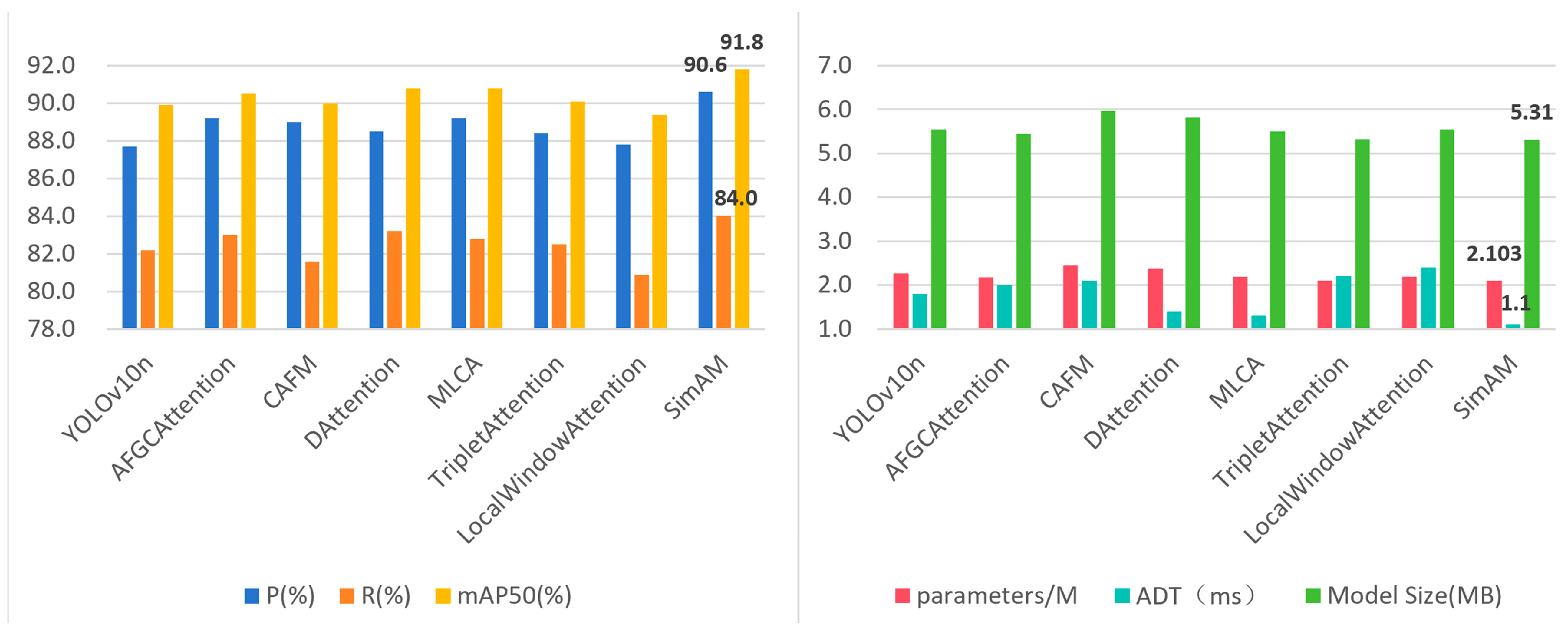
• The SimAM attention mechanism was integrated between the Backbone and Neck of YOLOv10n, and Complete Intersection Over Union Loss (CIOU) was replaced with Weighted Intersection over Union v3 (WIOUv3). These modifications notably enhanced performance in scenes involving occlusion, overlap, and congestion, minimizing false positives and missed detections without increasing additional parameters. The terminology utilized in this document is outlined in

  Table 1. Named terms list.

  Abbreviation	Meaning
  C2f-DWRR	C2f-Dilation-wise Residual-Reparam
  DWR	Dilation-wise Residual
  DRB	Dilated Reparam Block
  CIOU	Complete Intersection Over Union Loss
  WIOUv3	Weighted Intersection over Union v3
  NMS	non-maximum suppression
  ECA	Efficient Channel Attention
  DUC	Dense Upsampling Convolution

  .

2. Materials and Methods

2.1. Image Acquisition

Due to the absence of a public dataset for green pepper detection, a custom green pepper dataset was constructed in this study. Niujiao peppers served as the research subject. Data collection took place from 31 May to 10 June 2024, covering the pepper ripening period and incorporating images captured in sunny, rainy, and cloudy conditions. The collection site was the Danxi Longxin pepper plantation in Changzhi County, Changzhi City, Shanxi Province. Photographs were taken from multiple angles, under various lighting intensities and planting densities, specifically targeting green peppers in complex conditions such as direct lighting, backlighting, and occlusions. A Canon 60D camera was used, yielding 2555 green pepper images at 1080 × 1920 resolution in JPG format. To improve dataset quality, the images were manually classified, counted, and filtered based on field conditions, resulting in 11 distinct environmental categories and ensuring a balanced number of images for each experimental setting. Figure 1 shows examples of green pepper images under different environmental conditions.

2.2. Dataset Construction

To enhance the learning ability of deep neural networks and mitigate overfitting caused by insufficient sample diversity [22], the original image set-after manual classification-was subjected to data augmentation. Operations included noise addition, brightness adjustment, slicing, rotation, cropping, translation, and mirror flipping, ultimately expanding the dataset to 7755 images. The dataset was manually annotated using the LabelImg tool (version 1.8.6), with bounding boxes drawn in YOLO format. Subsequently, the dataset was split into training, validation, and test sets at a 7:1:2 ratio, resulting in 5428, 775, and 1552 images, respectively.

Table 2. Dataset image and annotation distribution.

Green Pepper Image and Annotation Count in Different Environments
Number	Environment Categories	Number of Images				Number of Annotations
		Training	Val	Test	Total	Training	Val	Test	Total
1	Overcast + fruit_branch + fruit_branch + fruit_branch	553	79	145	777	4013	627	1090	5730
2	Overcast + fruit_fruit + fruit_fruit	642	71	190	903	5551	550	1720	7821
3	Overcast + fruit_leaf	713	107	200	1020	5163	811	1517	7491
4	Blurry_target	264	41	79	384	2178	317	541	3036
5	Backlighting + fruit_branch + fruit_branch	318	36	81	435	2138	229	564	2931
6	Backlighting + fruit_fruit	293	40	90	423	3268	411	959	4638
7	Backlighting + fruit_leaf	320	46	93	459	2141	374	662	3177
8	Unobstructed	390	61	107	558	1806	285	537	2628
9	Frontlighting + fruit_branch + fruit_fruit	574	86	171	831	3576	473	1063	5112
10	Frontlighting + fruit_fruit	561	97	170	828	3830	680	1202	5712
11	Frontlighting + fruit_leaf	800	111	226	1137	5019	699	1356	7074
Total		5428	775	1552	7755	38,683	5456	11,211	55,350

shows the distribution of images and annotations across different environmental conditions.

2.3. YOLOv10 Network Architecture

YOLOv10, proposed by Wang et al. [23] in 2024, is the latest state-of-the-art single-stage object detection algorithm, overcoming key limitations of previous versions. Multiple innovative features significantly improve its performance and efficiency. The YOLOv10 architecture consists of three main parts-Backbone, Neck, and Head-responsible for feature extraction, feature fusion, and final computations. Figure 2 illustrates the YOLOv10 network structure.

To enhance the readability of Figure 2, different colors are used to represent various functional modules in the YOLOv10 network. Specifically, pink blocks represent standard convolutional layers (Conv), light blue blocks indicate C2f modules, purple blocks denote SCDown modules, green blocks correspond to C2f/CIB modules, gray blocks represent the SPPF module, cyan blocks indicate the PSA module, light yellow blocks are used for Concat operations, and light pink blocks represent Upsample operations.

The key advantage of YOLOv10 lies in its dual-head detection design, which removes the reliance on non-maximum suppression (NMS), significantly reducing inference latency and enhancing end-to-end deployment performance [24]. Depending on network depth and width, YOLOv10 provides six versions: n, s, m, b, l, and x. The YOLOv10n variant was selected here, as it is fast, accurate, and lightweight, making it well suited for complex field environments.

2.4. DSW-YOLO Network Architecture

In natural growth environments, green peppers vary significantly in size and shape, and leaves and branches closely match the fruit in color, causing mutual occlusion. In addition, multi-scale factors such as varying illumination intensity and angles can degrade model performance. To address feature extraction across different scales under field conditions, a lightweight DSW-YOLO model was proposed based on YOLOv10n by continually strengthening feature extraction. The structure of the optimized DSW-YOLO model is shown in Figure 3.

In Figure 3, the color scheme follows that of Figure 2 for consistency. Specifically, yellow blocks are used to represent the proposed C2f-DWRR modules, and red blocks indicate the SimAM attention mechanism integrated into the backbone.

First, to address the limited feature extraction ability of the original C2f structure under occlusion and varying lighting conditions, a lightweight C2f-DWRR module was introduced into the backbone to replace the Bottleneck modules in the 6th and 8th C2f blocks. Next, to compensate for the lack of an effective saliency mechanism in YOLOv10n, the parameter-free SimAM attention module was added to the final layer of the backbone. Finally, WIOUv3 was adopted to replace the original CIOU, which performs poorly when predicted boxes are far from the ground truth, by introducing adaptive penalties to improve regression accuracy and convergence during training. These enhancements integrate multiple lightweight modules with complementary strengths. Through a multi-strategy fusion design, the model demonstrates stronger robustness in scenarios involving occlusion, scale variation, and complex illumination, while balancing detection performance and deployment efficiency on edge devices.

2.4.1. Construction of the C2f-DWRR Module

To effectively capture multi-scale information from green pepper images and enhance the network’s feature extraction capability, a C2f-DWRR module is introduced. Although the C2f module in YOLOv10 enables feature fusion, some backbone layers still suffer from channel redundancy and limited receptive field. To address this, we integrate a Dilation-wise Residual-Reparam (DWRR) module-combining dilated convolution (DWR) and re-parameterization (DRB)-into the C2f block via class inheritance, replacing the original Bottleneck. The resulting C2f-DWRR module enhances multi-scale feature representation while maintaining computational efficiency, improving the model’s robustness to occlusion and scale variation. The new module, termed C2f-DWRR, is illustrated in Figure 4.

In Figure 4, yellow blocks represent the DWRR module, light green blocks indicate the split module, light pink blocks denote the convolution branches, and light yellow blocks correspond to the Concat module.

It was observed that both the DRB block proposed by Ding et al. [25] in UniRepLKNet and the DWR block introduced by Wei et al. [26] in DWRSeg adopt dilated convolutions for an expanded receptive field, utilizing various dilation rates across multiple layers. However, the deep convolutional layers in the original DWR framework (such as D-3 and D-5 dilated convolutions) still lead to certain computational inefficiencies. To address this issue, we propose replacing deep convolutions with Dilated Reparameterization Blocks (DRB). The specific reasons are as follows:

(1)

DRB module enhances multi-scale feature extraction capability: The DRB module can simultaneously capture fine-grained local features and broader spatial context by using gradually increasing dilation rates across multiple layers, thereby enhancing the ability to extract multi-scale features.

(2)

Trade-off between accuracy and efficiency: Compared to the higher computational cost of deep convolutions with larger input feature maps, DRB reduces the number of parameters and computational burden through reparameterization techniques, while almost maintaining the accuracy of feature extraction.

(3)

Maintaining the basic feature extraction characteristics of the DWR module: Although the computational efficiency is optimized, the first branch of the DWRR module still uses convolution layers with a dilation rate of zero, ensuring that the basic operations and feature extraction properties of the original structure are preserved. This balance between efficiency and functionality is crucial for ensuring that the model captures key features.

In summary, replacing deep convolutions in DWR with the DRB module aims to optimize computational efficiency while maintaining multi-scale feature extraction capabilities and minimizing the impact on model accuracy, making the DWRR module an efficient alternative to the original DWR structure. The DRB model structure is shown in Figure 5a, the DWR model structure in Figure 5b, and the DWRR model structure in Figure 5c.

In Figure 5, the background of subfigure (a) is light yellow, representing the DRB module. In subfigure (b), pink, green, and purple blocks represent the three parallel branches in the DWR module. In subfigure (c), the yellow blocks highlight the embedded DRB modules within the DWRR structure.

The DWRR module is composed of the following components:

• DRB: DRB achieves a similar effect to large kernel convolution by using multiple smaller dilated kernels. The input first goes through a 9 × 9 kernel, followed by two 5 × 5 kernels and two 3 × 3 kernels with increasing dilation rates. Batch normalization (BN) boosts training efficiency and stability. This approach reconfigures the layers to act like a single large-kernel convolution, expanding the receptive field and improving spatial feature extraction while keeping the model efficient in terms of parameters and computation.
• DWR: The DWR module improves multi-scale information collection using a two-step process-Regional Residualization (RR) and Semantic Residualization (SR)-to capture detailed features. In the first step (RR), it generates multi-scale feature maps with 3 × 3 convolutions, BN, and ReLU, enhancing the ability to process information. In the second step (SR), these maps are grouped into clusters with similar features using morphological filtering. Convolutions with different dilation rates adjust the features, improving spatial analysis. The results are combined and passed through a 1 × 1 convolution to reduce complexity and parameters. Finally, the original input is added back to the output through a residual connection, boosting the network’s learning and stability. This design makes the DWR module ideal for high-precision, efficient deep learning tasks.

2.4.2. SimAM Attention Mechanism

To address common challenges in green pepper harvesting, such as severe fruit occlusion, high color similarity between leaves and fruits, and uneven illumination, and to guide the model in refocusing and enhancing key feature regions, suppressing irrelevant background interference, and strengthening responses in target-related areas, we introduced the SimAM attention module between the YOLOv10 backbone (feature extraction) and neck (feature fusion) (Figure 6).

SimAM is a simple, lightweight attention mechanism that improves efficiency by using a three-dimensional weighted attention process. It combines spatial and channel features without adding extra parameters. It helps the model focus on the most relevant information for visual tasks.

Drawing on the collaborative interaction of spatial and channel domains in the human brain [27], Yang et al. introduced SimAM in 2021 [28]. In visual neuroscience, active neurons with strong spatial inhibition exert a notable suppressive effect on surrounding neurons [29]. Based on this principle, SimAM calculates an energy function to gauge each neuron’s contribution, then dynamically adjusts weights to highlight key information and suppress irrelevant features.

The energy function for SimAM is defined as follows:

$${\mathrm{e}}_{\mathrm{t}}\left({\mathrm{w}}_{\mathrm{t}},{\mathrm{b}}_{\mathrm{t}},\mathrm{y},{\mathrm{x}}_{\mathrm{i}}\right)=\left({\mathrm{y}}_{\mathrm{t}}-\widehat{\mathrm{t}}\right)+{\displaystyle \frac{1}{\mathrm{M}-1}}\sum ^{\mathrm{M}-1}{\left({\mathrm{y}}_0-{\widehat{\mathrm{x}}}_{\mathrm{i}}\right)}^2$$

(1)

In this model, $\mathrm{t}$ represents the target neuron, ${\mathrm{x}}_{\mathrm{i}}$ denotes other neurons, ${\mathrm{w}}_{\mathrm{t}}$ and ${\mathrm{b}}_{\mathrm{t}}$ are the weight and bias, respectively. $\mathrm{M}$ is the total number of neurons. Minimizing the given formula helps improve the ability of neurons within the same channel to distinguish different features, enhancing their linear discriminative power. To simplify this process, binarized labels (i.e., ${\mathrm{y}}_{\mathrm{t}}$ and ${\mathrm{y}}_{\mathrm{o}}$ set to 1 and −1) are employed, and a regularization term is added, yielding the final energy function:

$${\mathrm{e}}_{\mathrm{t}}\left({\mathrm{w}}_{\mathrm{t}},{\mathrm{b}}_{\mathrm{t}},\mathrm{y},{\mathrm{x}}_{\mathrm{i}}\right)={\displaystyle \frac{1}{\mathrm{M}-1}}\sum _{\mathrm{i}=1}^{\mathrm{M}-1}{\left(-1-\left({\mathrm{w}}_{\mathrm{t}}{\mathrm{x}}_{\mathrm{i}}+{\mathrm{b}}_{\mathrm{t}}\right)\right)}^2+{\left(-1-\left({\mathrm{w}}_{\mathrm{t}}\mathrm{t}+{\mathrm{b}}_{\mathrm{t}}\right)\right)}^2+\lambda {\mathrm{w}}_{\mathrm{t}}^2$$

(2)

In this equation, $\lambda$ serves as the balancing parameter for regularization and possesses an analytical solution; the formula is as follows:

$${\mathrm{w}}_{\mathrm{t}}=-{\displaystyle \frac{2\left(\mathrm{t}-{\mu }_{\mathrm{t}}\right)}{{\left(\mathrm{t}-{\mu }_{\mathrm{t}}\right)}^2+2{\sigma }_{\mathrm{t}}^2+2\lambda }}$$

(3)

$${\mathrm{b}}_{\mathrm{t}}=-{\displaystyle \frac{1}{2}}\left(\mathrm{t}+{\mu }_{\mathrm{t}}\right){\mathrm{w}}_{\mathrm{t}}$$

(4)

In this formula, ${\mu }_{\mathrm{t}}$ and ${\sigma }_{\mathrm{t}}^2$ denote the mean and variance of all neurons in the target channel except for, respectively, thereby yielding the expression for the minimum energy:

$${\mathrm{e}}_{\mathrm{t}}^{\mathrm{*}}={\displaystyle \frac{4\left({\widehat{\sigma }}^2+\lambda \right)}{{\left(\mathrm{t}-\widehat{\mu }\right)}^2+2{\widehat{\sigma }}^2+2\lambda }}$$

(5)

Equation (5) indicates that the lower the energy of a neuron, the more pronounced its difference from the surrounding neurons, and consequently, the greater its importance. Therefore, a neuron’s importance can be determined by ${\displaystyle \frac{1}{{\mathrm{e}}_{\mathrm{t}}^{\mathrm{*}}}}$. To effectively highlight key features, the attention mechanism should reinforce these features.

SimAM avoids the additional computational overhead typically required by traditional attention mechanisms through a parameter-free design. Its dynamic weight adjustment mechanism relies on the feature information of the existing network, thus reducing extra computational steps. Unlike mechanisms that require substantial computation and parameter learning, SimAM enhances feature focus optimization without the need for adding complex computational paths or extra computational resource consumption. Therefore, it can significantly improve model performance under resource-constrained conditions while avoiding any impact on GPU/CPU utilization.

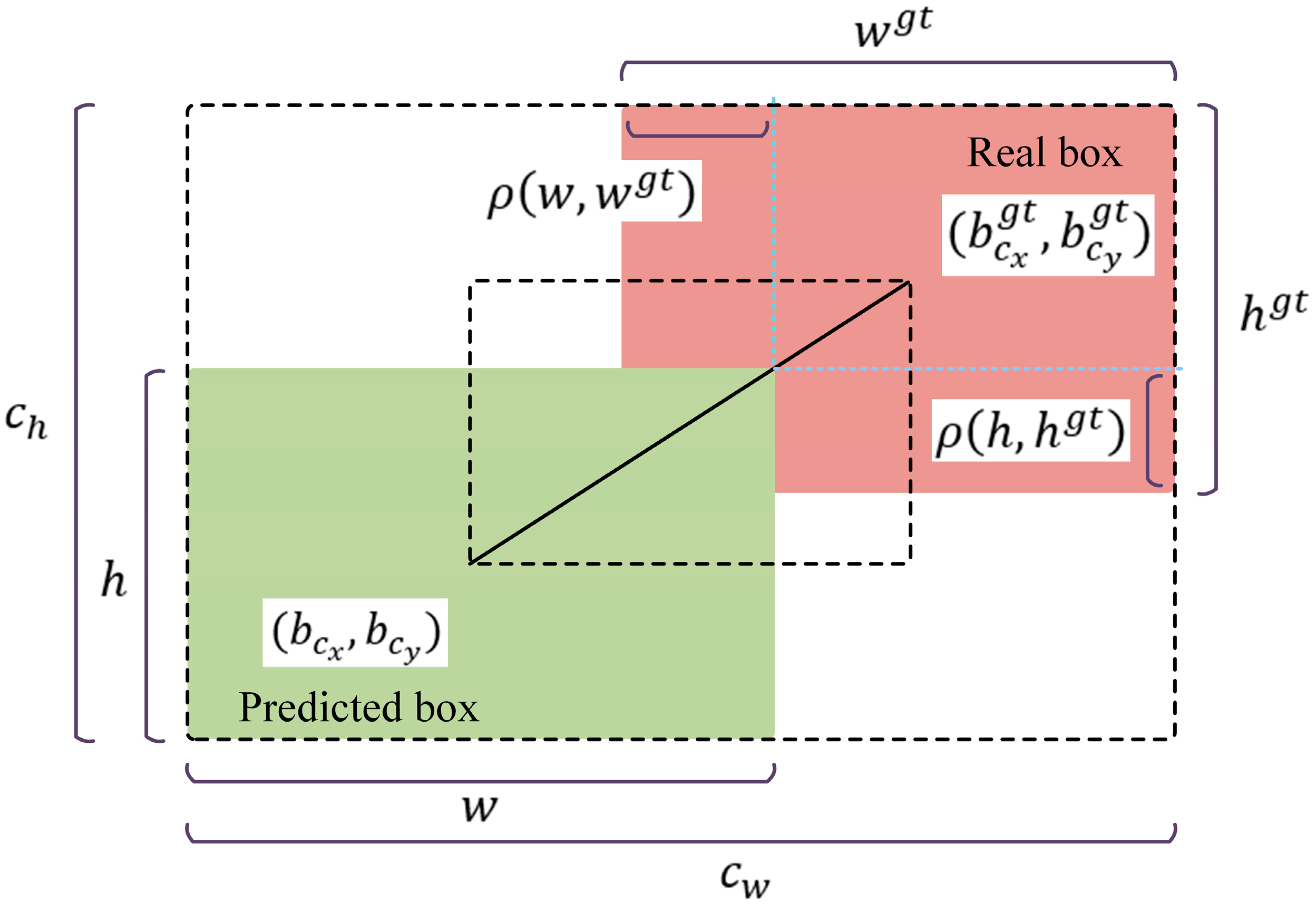
2.4.3. WIoUv3 Loss Function

The standard CIOU used in the YOLOv10n baseline has notable limitations: (1) it fails to distinguish between easy and hard samples, which is critical for green pepper detection in complex field environments; and (2) it inadequately penalizes differences when bounding boxes share the same aspect ratio but vary in size. To overcome these issues, WIoUv3 is adopted to replace CIOU, providing more adaptive and precise localization optimization.

WIoUv3 is a bounding box localization loss function proposed by Tong et al. [30]. WIoUv3 takes into account the aspect ratio, centroid distance, and overlap area, and adds a dynamic focusing mechanism. For low-quality samples, it evaluates the anchor box quality using an outlier value, and $\beta$ adjusts the focusing factor $\mathrm{r}$. When the quality $\beta$ is low (high outlier value), the focusing factor $\mathrm{r}$ decreases, reducing the impact of poor-quality anchor boxes. This dynamic adjustment of loss weights helps the model handle sub-optimal samples better, improving overall performance. The WIoUv3 formulas are presented in Equations (6)–(10), with the associated parameters illustrated in Figure 7.

$${\mathrm{L}}_{\mathrm{W}\mathrm{I}\mathrm{o}\mathrm{U}\mathrm{v}3}=\mathrm{r}\times {\mathrm{R}}_{\mathrm{W}\mathrm{I}\mathrm{o}\mathrm{U}}\times {\mathrm{L}}_{\mathrm{I}\mathrm{o}\mathrm{U}}$$

(6)

$$\mathrm{r}={\displaystyle \frac{\beta }{\delta {\alpha }^{\beta -\delta }}}$$

(7)

$${\mathrm{R}}_{\mathrm{W}\mathrm{I}\mathrm{o}\mathrm{U}}=\mathrm{e}\mathrm{x}\mathrm{p}{\displaystyle \frac{{\left({\mathrm{b}}_{{\mathrm{C}}_{\mathrm{x}}}^{\mathrm{g}\mathrm{t}}-{\mathrm{b}}_{{\mathrm{c}}_{\mathrm{x}}}\right)}^2+{\left({\mathrm{b}}_{{\mathrm{C}}_{\mathrm{y}}}^{\mathrm{g}\mathrm{t}}-{\mathrm{b}}_{{\mathrm{c}}_{\mathrm{y}}}\right)}^2}{{\mathrm{c}}_{\mathrm{w}}2+{\mathrm{c}}_{\mathrm{h}}2}}$$

(8)

$$L_{IoU}=1-IoU$$

(9)

$$\beta ={\displaystyle \frac{{\mathrm{L}}^{\mathrm{*}}\mathrm{I}\mathrm{o}\mathrm{U}}{\overline{{\mathrm{L}}_{\mathrm{I}\mathrm{o}\mathrm{U}}}}}\in [0,+\mathrm{\infty })$$

(10)

WIoUv3 leverages its dynamic focusing mechanism to assess the quality of anchor boxes through outlier analysis, effectively mitigating the impact of blurred scenes and noisy annotations while avoiding unnecessary penalties due to minor geometric differences from manual labeling. Furthermore, WIoUv3 incorporates a monotonic focusing coefficient ${\mathrm{L}}_{\mathrm{I}\mathrm{o}\mathrm{U}}^{\mathrm{*}}$ to enhance convergence speed. At the same time, the dynamic weighting mechanism can reduce the interference of noise labeling on model training, which is helpful to improve the robustness and generalization ability of the model. Experimental results demonstrate that when processing green pepper samples in complex environments, WIoUv3 reduces loss values, accelerates convergence, and significantly improves model robustness, exhibiting clear performance advantages during dataset training.

2.5. Experimental Platform Configuration and Training Strategy

The training hardware for this experiment primarily consisted of an Intel Core i5-12490F CPU @3.0 GHz with 12 cores, an NVIDIA GeForce RTX 3060 Ti 8G GPU, and 16 GB of RAM. Regarding the software environment, a deep learning framework was built on the Windows 11 operating system using Python 3.9.18, Cuda 11.6, and Pytorch 1.13.1, with PyCharm as the programming platform. During training, YOLOv10n.pt was selected as the pre-trained weight, and the self-built green pepper dataset was used with an input image size of 640 × 640 pixels, employing the stochastic gradient descent (SGD) algorithm. After debugging and testing, the specific training parameters are presented in

Table 3. Training parameters.

Training Parameters	Values
Initial learning rate	0.01
Number of images per batch	32
Number of epochs	1000
Optimizer	SGD
Optimizer momentum	0.937
Optimizer weight decay rate	0.0005
Image input size	640 × 640

.

2.6. Evaluation Metrics

To achieve real-time detection of green pepper fruits in complex environments and enable subsequent edge deployment, it is crucial to optimize the model’s detection accuracy, detection speed, and model size. For detection accuracy, focus should be placed on metrics such as P, R, mAP50, and mean average precision over the IoU threshold range of 0.5–0.95 (mAP50-95), among others. In terms of detection speed, the parameter count and average detection time (ADT) must be considered. AP measures the combined performance of precision and recall at various confidence thresholds, while mean average precision (mAP) provides a more comprehensive reflection of overall performance in multi-class object detection. The mAP50 metric indicates that if the IoU between a detected object and its ground-truth box exceeds 0.5, the target is considered successfully detected. The formulas for calculating P, R, and mAP50 are given in Equations (11)–(14).

$$Precision={\displaystyle \frac{TP}{TP+FP}}$$

(11)

$$Recall={\displaystyle \frac{TP}{TP+FN}}$$

(12)

$$AP={\int }_0^{1}P\left(R\right)dr$$

(13)

$${mAP}_{50}={\displaystyle \frac{1}{n}}\sum _{i=1}^n{AP}_{50,i}$$

(14)

Here, TP denotes the number of true positive instances correctly detected by the model, FP denotes the number of negative instances mistakenly detected as positive, and FN denotes the number of positive instances missed by the model. P represents precision, R represents recall, P(R) represents the maximum precision at a recall level of r, and n is the total number of classes.

3. Results

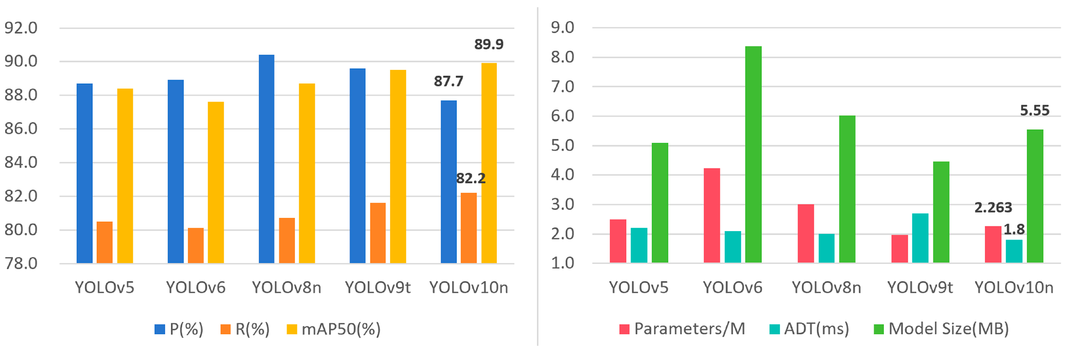
3.1. Analysis of Comparative Results of YOLO-Series Algorithms

To evaluate the performance of basic YOLO models in green pepper recognition, the dataset from Section 2.2 was used under identical conditions to compare YOLOv5n, YOLOv6n, YOLOv8n, YOLOv9t, and YOLOv10n. The evaluation metrics included P, R, mAP50, mAP50-95, parameters, ADT, and model size. The comparative results of these baseline models are shown in Figure 8.

As shown in Figure 8, YOLOv10n demonstrates the best overall performance among lightweight YOLO models, with outstanding R and mAP50 results, the shortest ADT, and balanced parameters and model size. Detailed numerical comparisons of the baseline models are provided in

Table 4. Baseline model comparison experiment results.

Number	Algorithm	P (%)	R (%)	mAP50 (%)	mAP50-95 (%)	Parameters/M	ADT (ms)	ModelSize (MB)
1	YOLOv5n	88.7	80.5	88.4	64.3	2.503	2.2	5.09
2	YOLOv6n	88.9	80.1	87.6	65.2	4.234	2.1	8.38
3	YOLOv8n	90.4	80.7	88.7	65	3.006	2.0	6.03
4	YOLOv9t	89.6	81.6	89.5	66.5	1.971	2.7	4.46
5	YOLOv10n	87.7	82.2	89.9	65.9	2.263	1.8	5.55

.

YOLOv6n yields the lowest R (80.1%) and mAP50 (87.6%) across all evaluated models, indicating inferior localization and confidence performance. YOLOv5n shows moderate performance on all metrics, making it less competitive in practical deployment. Although YOLOv8n achieves the highest precision (P = 87.5%), it suffers from a relatively low R of 80.7% and presents a larger model size and parameter count, which may hinder real-time deployment. While YOLOv9t has the smallest parameter size, its mAP50 (89.5%) and R (81.6%) are still slightly lower than those of YOLOv10n, by 0.4% and 0.6%, respectively. In contrast, YOLOv10n not only achieves the best R (82.2%) and mAP50 (89.9%) but also delivers the shortest ADT (1.8 ms), reflecting its superior efficiency and accuracy.

In summary, YOLOv10n demonstrates the most balanced and effective performance across all metrics, and is thus selected as the baseline model for subsequent improvements targeting detection accuracy and lightweight optimization.

3.2. C2f Module Optimization Results and Analysis

To verify the effectiveness of the C2f-DWRR module on the green pepper dataset, the following experiments were designed. First, the FasterBlock from FasterNet [31], the ODConv dynamic convolution block [32], the ContextGuided block from CGNet [33], as well as the DRB and DWR blocks mentioned in Section 2.4.1, were each used to replace and integrate YOLOv10n’s C2f block, forming five modules: C2f-Faster, C2f-ODConv, C2f-ContextGuided, C2f-DWR, and C2f-DRB. These enhanced C2f blocks were then compared against the proposed C2f-DWRR module, using the green pepper dataset constructed in Section 2.2 and the training strategy described in Section 2.5. Experiment 1 shows the performance of the original model without C2f optimization. An intuitive comparison of C2f optimization is illustrated in Figure 9.

As shown in Figure 9, the C2f-DWRR module significantly improves model accuracy while reducing both parameters and model size, confirming its effectiveness. Detailed experimental values for the C2f optimization and analysis are listed in

Table 5. C2f module optimization experiment results.

Number	Algorithm	P (%)	R (%)	mAP50 (%)	mAP50-95 (%)	Parameters /M	ADT (ms)	Model Size (MB)
1	C2f	87.7	82.2	89.9	65.9	2.263	1.8	5.69
2	C2f-Faster	87.4	78.0	87.3	62.5	1.780	2.1	4.73
3	C2f-ODConv	88.6	80.7	88.5	64.3	2.317	2.8	5.84
4	C2f-ContextGuided	87.1	79.2	87.8	62.4	1.644	2.0	4.50
5	C2f-DRB	88.4	81.8	89.6	66.0	1.965	2.2	5.20
6	C2f-DWR	90.5	83.6	91.5	67.2	2.204	2.2	5.59
7	C2f-DWRR	90.0	84.3	91.7	69.3	2.103	2.2	5.44

.

Experiments 2 and 4 indicate that although C2f-Faster and C2f-ContextGuided significantly reduce parameters and model size, their accuracy metrics decline compared to the original model. Results from Experiment 3 show that C2f-ODConv improves P by 0.9 percentage points but decreases R, mAP50, and mAP50-95 by 1.5, 1.4, and 1.6 points, respectively, and increases parameters, model size, and ADT-extending detection time by 1ms, which fails to meet real-time demands. Experiment 5 reveals that C2f-DRB achieves similar P, R, mAP50, and mAP50-95 to the original model while reducing parameters and model size. Experiment 6 demonstrates that C2f-DWR raises P, R, mAP50, and mAP50-95 by 2.8, 1.4, 1.6, and 1.3 points, respectively, with parameters and model size remaining comparable to the original. Experiment 7 confirms that the C2f-DWRR module integrates the advantages of DRB and DWR, increasing P, R, mAP50, and mAP50-95 by 2.3, 2.1, 1.8, and 3.4 points, respectively, while also reducing parameters and model size.

In summary, the C2f-DWRR module improves accuracy while lowering the parameter count and model size, offering robust support for further research.

3.3. Attention Mechanism Optimization Results and Analysis

To assess the impact of integrating the SimAM attention mechanism between the Backbone and Neck on detection performance, a comparative experiment was conducted under the same conditions against six different attention modules (AFGC [34], CAFM [35], DAT [36], MLCA [37], TP [38], and LWA [39]). Figure 10 shows a comparison of the optimization results for each attention mechanism.

As shown in Figure 10, integrating SimAM significantly improves the model’s recognition accuracy in complex scenarios, reduces detection time, and enhances sensitivity and responsiveness to critical information. Detailed numerical results regarding the impact of different attention mechanisms on model performance are presented in

Table 6. Attention mechanism optimization experiment results.

Number	Algorithm	P (%)	R (%)	mAP50 (%)	mAP50-95 (%)	Parameters /M	ADT (ms)	Model Size (MB)
1	YOLOv10n	87.7	82.2	89.9	65.9	2.263	1.8	5.55
2	YOLOv10n- C2f-DWRR	90.0	84.3	91.7	69.3	2.103	2.2	5.31
3	AFGCAttention	89.2	83.0	90.5	67.0	2.169	2.0	5.44
4	CAFM	89.0	81.6	90.0	65.0	2.449	2.1	5.97
5	DAttention	88.5	83.2	90.8	67.4	2.370	1.4	5.82
6	MLCA	89.2	82.8	90.8	66.5	2.197	1.3	5.50
7	TripletAttention	88.4	82.5	90.1	65.5	2.103	2.2	5.32
8	LocalWindow Attention	87.8	80.9	89.4	64.5	2.197	2.4	5.55
9	SimAM	90.6	84.0	91.8	68.5	2.103	1.1	5.31

.

According to Table 6, incorporating SimAM into YOLOv10n boosts P, R mAP50, and mAP50-95 by 2.9%, 1.8%, 1.9%, and 2.6%, respectively, while reducing parameters, ADT, and model size. Compared to YOLOv10n with C2f-DWRR, SimAM increases P and mAP50 by 0.6% and 0.1%, respectively, with faster ADT and unchanged model size, highlighting its efficiency in resource-constrained, real-time applications. Furthermore, relative to AFGC, CAFM, DAT, MLCA, TP, and LWA attention mechanisms, SimAM maintains a lead in P R, mAP50, and mAP50-95, while also further decreasing or shortening parameters, model size, and ADT.

In summary, embedding the SimAM attention mechanism between the Backbone and Neck effectively improves model P and R while balancing lightweight design and real-time performance, thus avoiding wasting GPU/CPU computing power. Its enhancements to spatial- and channel-domain feature extraction offer strong support for subsequent improvements and research.

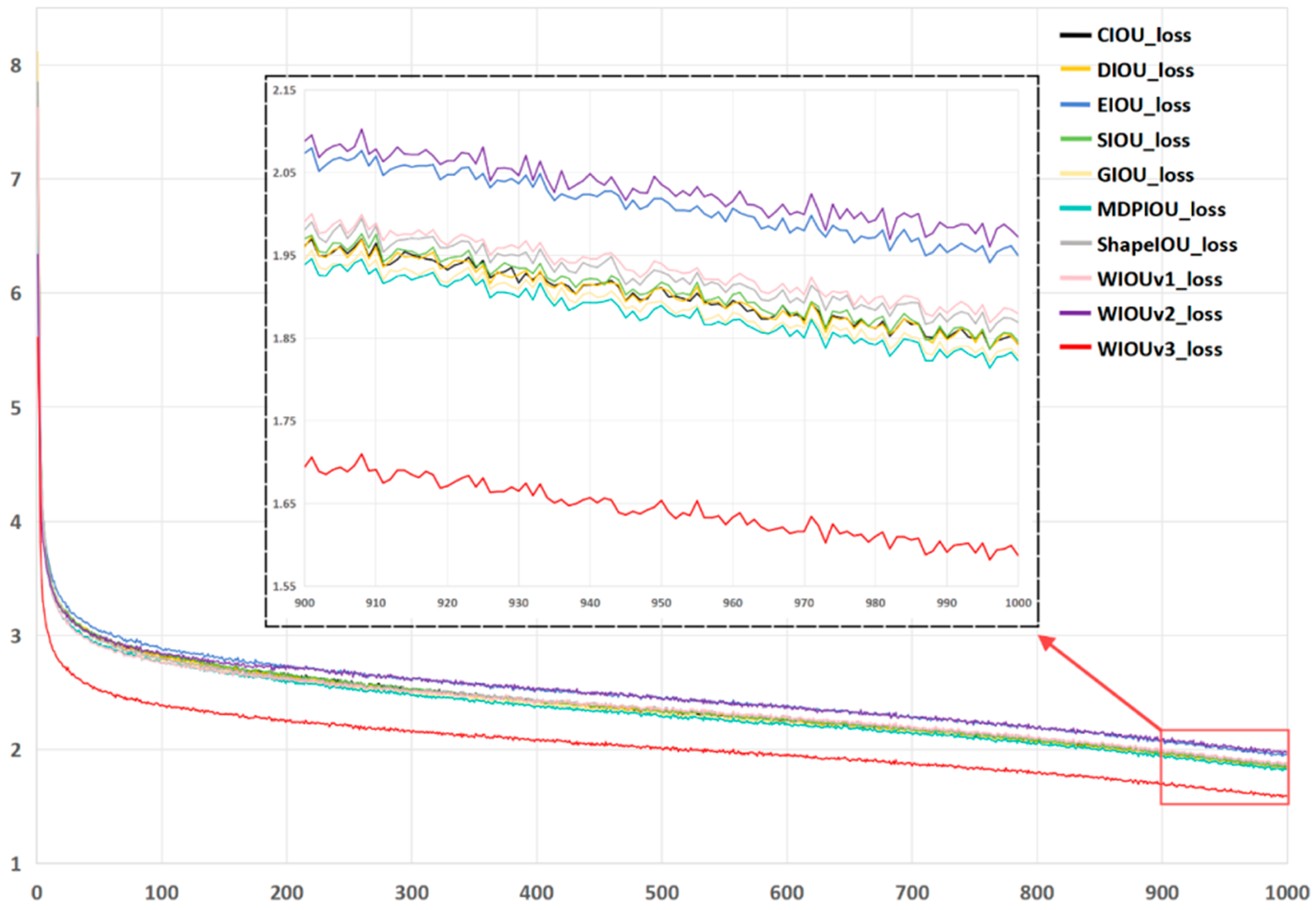
3.4. Loss Function Optimization Results and Analysis

To improve the accuracy of bounding box regression and mitigate penalties caused by inaccurate annotations or geometric inconsistencies, the CIOU in YOLOv10n was replaced with DIOU, EIOU, SIOU, GIOU, MDPIOU, ShapeIOU, and WIOUv1, WIOUv2, and WIOUv3 for comparative evaluation. The training loss curves for each loss function are shown in Figure 11.

As shown in Figure 11, WIoUv3 achieves the lowest loss value and fastest convergence among all tested methods. This indicates that the network benefits from WIoUv3’s improved localization quality and stable learning process. Compared with traditional IOU-based losses, WIoUv3 introduces a dynamic focusing mechanism that adaptively weights anchor box contributions during training. This helps the model better distinguish high-quality anchors while suppressing noisy or ambiguous samples, thus facilitating more robust training.

As shown in

Table 7. Loss function optimization experiment results.

Loss Function	P (%)	R (%)	mAP50 (%)	mAP50-95 (%)
CIOU	90.6	84.0	91.8	68.5
WIOU-V3	90.6	84.9	92.1	69.3
DIOU	91.3	83.6	91.9	68.9
EIOU	89.4	82.4	90.3	66.2
SIOU	89.8	83.9	91.9	68.3
GIOU	90.4	82.4	90.9	67.9
MDPIOU	89.5	84.9	91.8	68.8
ShapeIOU	89.5	84.1	91.0	67.7
WIOU-V1	89.8	82.3	91.0	67.1
WIOU-V2	89.6	83.7	91.5	68.4

, WIOUv3 achieves recall, mAP50, and mAP50-95 values of 84.9%, 92.1%, and 69.3%, respectively-improving these three metrics by 0.9%, 0.3%, and 0.8% over the baseline model’s CIOU, with no change in precision. Although DIOU reaches a precision of 91.3%, its recall, mAP50, and mAP50-95 are 1.3%, 0.2%, and 0.4% lower than those of WIOUv3. Moreover, compared with EIOU, SIOU, GIOU, MDPIOU, ShapeIOU, WIOUv1, and WIOUv2, WIOUv3 leads all metrics.

In summary, the model utilizing WIOUv3 exhibits standout performance during training, achieving the highest detection accuracy overall.

3.5. Ablation Test

To further validate the effectiveness of each improvement module and to quantitatively assess their individual and combined contributions to model performance, the following ablation experiments were conducted under identical conditions. The evaluation metrics described in Section 2.6 were used. In these experiments, “√” indicates that the model includes the corresponding module, whereas “×” indicates it does not. Detailed results are presented in

Table 8. Ablation test results of each improved module.

Number	Base Line	C2f- DWRR	SimAM	WIOUv3	P (%)	R (%)	mAP50 (%)	mAP50-95 (%)	Parameters /M	ADT (ms)	Model Size (MB)
1	✔				87.7	82.2	89.9	65.9	2.263	1.8	5.55
2	✔	✔			90.0	84.3	91.7	69.3	2.103	2.2	5.31
3	✔		✔		86.7	80.3	88.5	63.9	2.907	2.6	7.96
4	✔			✔	89.4	81.5	90.1	65.4	2.265	2.3	5.56
5	✔	✔	✔		90.6	84.0	91.8	68.5	2.103	1.1	5.31
6	✔	✔	✔	✔	90.6	84.9	92.1	69.3	2.103	1.1	5.31

. Experiment 1 demonstrates the performance of the basic YOLOv10n model for green pepper detection; Experiments 2, 3, and 4 each show the effects of separately adding C2f-DWRR, SimAM, and WIOUv3 to YOLOv10n; and Experiments 2, 5, and 6 illustrate the step-by-step integration of these improvement modules into YOLOv10n.

Experiment 2 evaluates the impact of the C2f-DWRR module on the YOLOv10n baseline. The results indicate that it optimizes computation speed and enhances multi-scale feature extraction, improving P, R, mAP50, and mAP50-95 by 2.3%, 2.1%, 1.8%, and 3.4%, respectively. Meanwhile, parameters and model size decrease by 0.16M and 0.246MB. Although the ADT increases by 0.4 ms-mainly due to added convolution layers in the C2f-DWRR module-it imposes minimal effect on overall parameters and model size.

Experiment 3 explores the effect of introducing SimAM attention alone. The results reveal a decline in P and an increase in parameter count and model size. This may stem from SimAM’s high computational complexity under large channel counts and large feature maps, whereas the lightweight C2f module of YOLOv10n primarily targets reduced overhead. Directly integrating SimAM could increase the computational load and reducing model performance. Experiment 4 assesses the effect of replacing the CIOU with WIOUv3. This replacement increases P by 1.7% and mAP50 by 0.2%, yet R and mAP50-95 decrease by 0.7% and 0.5%, respectively. Analyses suggest WIOUv3 may favor high-confidence targets to reduce false positives, but it can also lower the recall rate for certain objects.e model performance.

Further analysis of Experiments 2, 3, and 5 shows that incrementally introducing C2f-DWRR and SimAM into YOLOv10n increases P, R, mAP50, and mAP50-95 by 2.9%, 1.8%, 1.9%, and 2.6%, respectively, while reducing parameters, average detection time (ADT), and model size by 0.16 M, 0.7 ms, and 0.241 MB. These results indicate that C2f-DWRR improves feature processing via expandable residuals and structural re-parameterization, while SimAM’s 3D-weighted attention mechanism strengthens feature selectivity and reduces computational load. Combining these modules further optimizes detection accuracy and efficiency.

Based on Experiments 1, 2, 5, and 6, incrementally incorporating C2f-DWRR, SimAM, and WIOUv3 into YOLOv10n boosts precision, recall, mAP50, and mAP50-95 by 2.9%, 2.7%, 2.2%, and 3.4%, respectively, relative to the original model, while reducing parameters, ADT, and model size by 1.6 M, 0.7 ms, and 0.242 MB.

In summary, progressively integrating C2f-DWRR, SimAM, and WIOUv3 significantly enhances detection accuracy and computational efficiency, confirming the effectiveness of each improvement module.

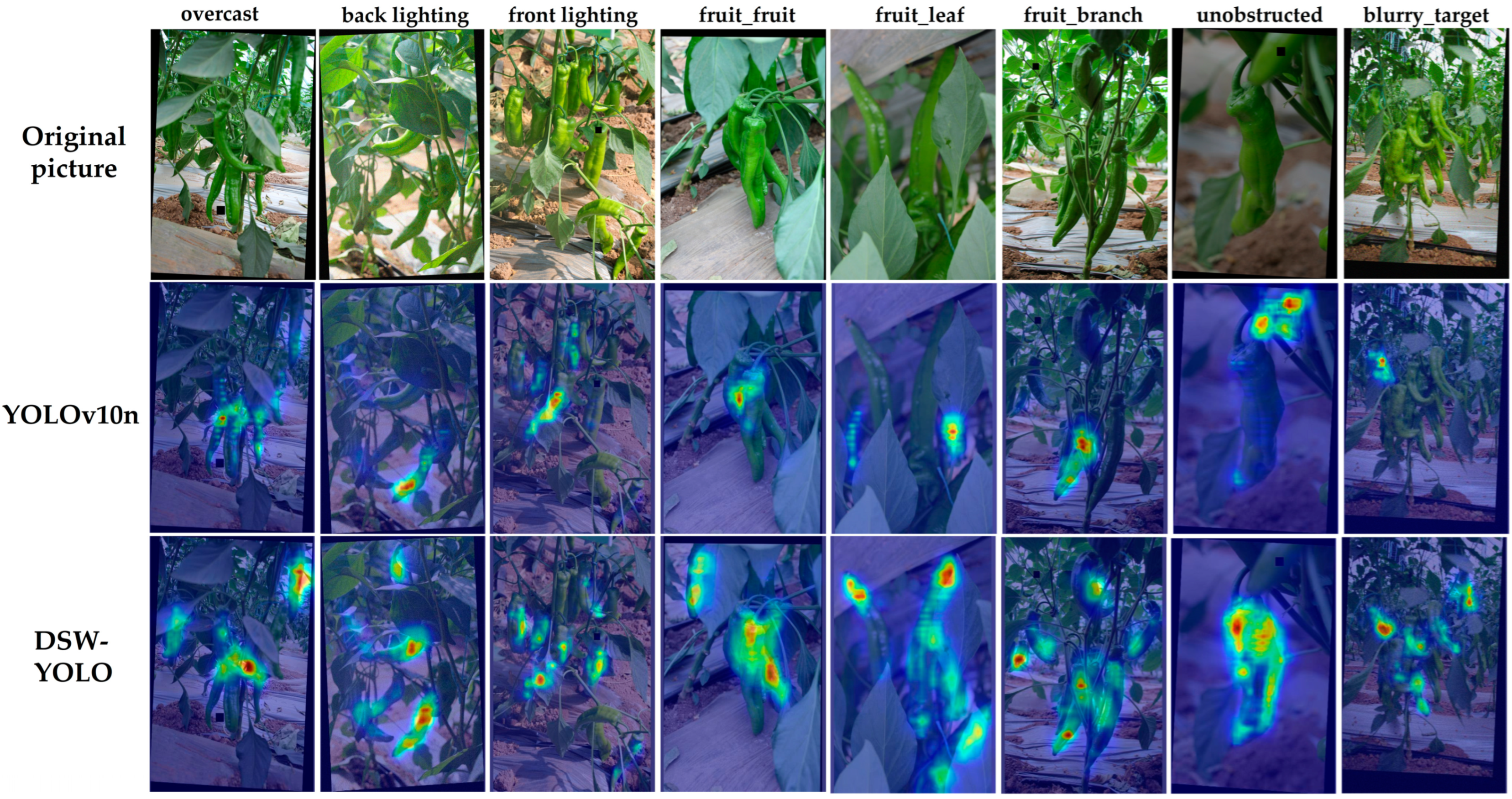
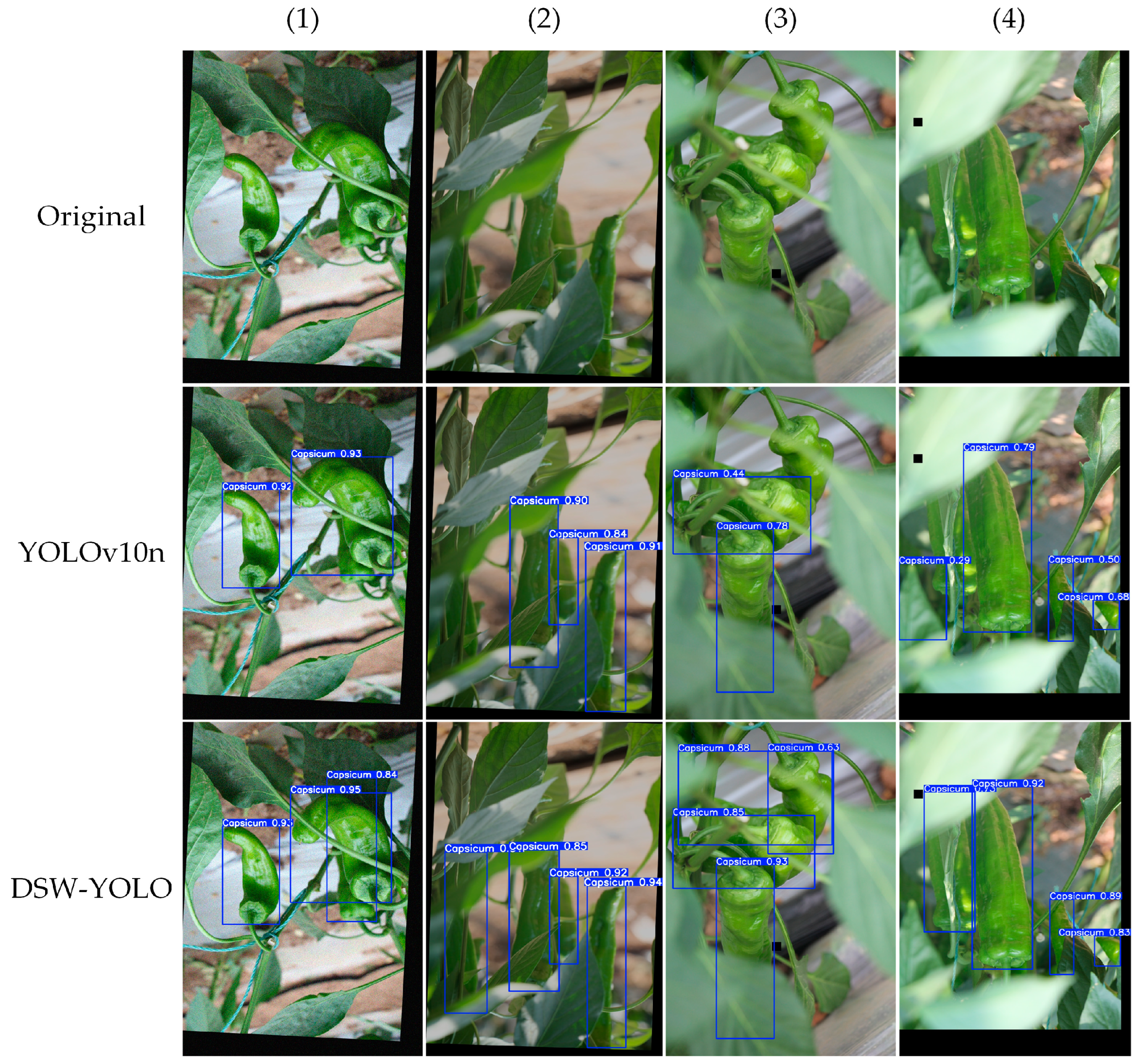
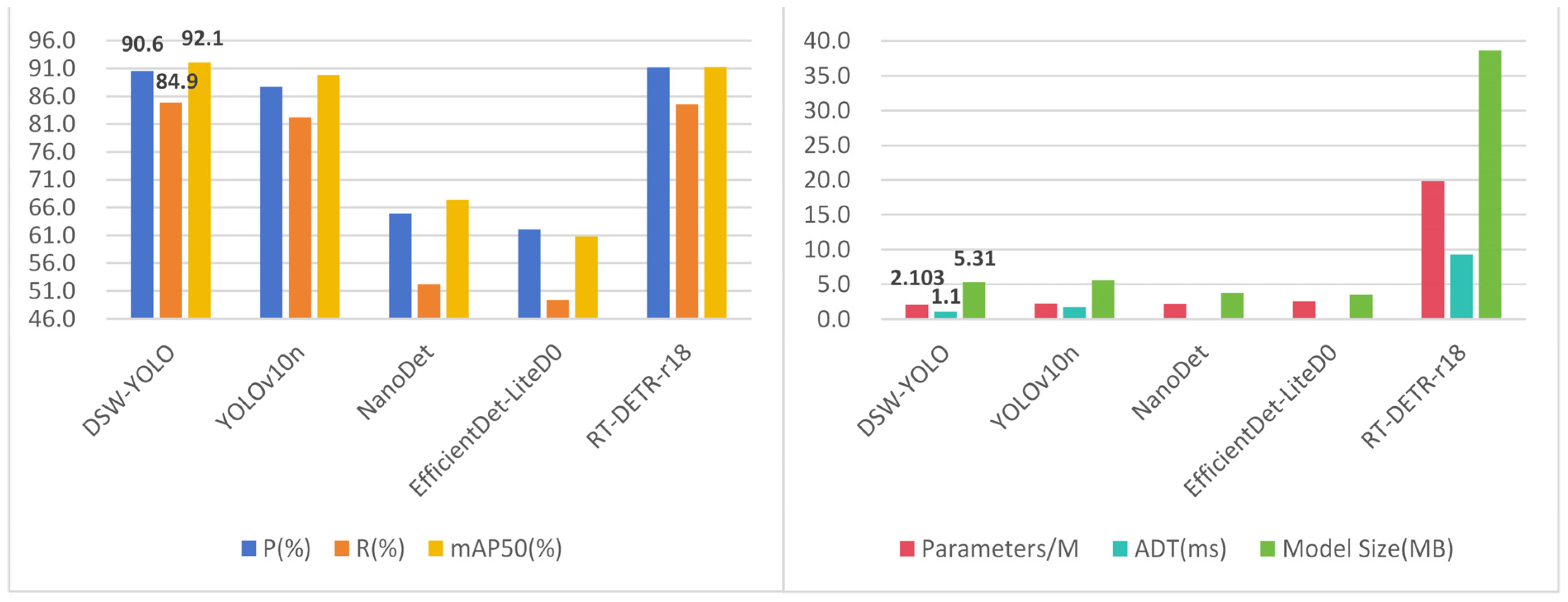
3.6. Final Optimized Model Analysis

To verify the effectiveness of DSW-YOLO in multi-scale green pepper detection under complex conditions, LayerCAM was used for visualization [40]. LayerCAM generates fine-grained heatmaps by fusing multi-layer feature information, providing more precise results than Grad-CAM in complex backgrounds and small-object detection [41]. The heatmap employs color coding to represent the importance of different regions, ranging from cooler tones (blue) to warmer tones (red), where red indicates high attention and blue indicates low attention. Figure 12 shows the heatmaps of the test set before and after the improvements.

As shown in Figure 12, whether under overcast conditions, backlit sunlight, direct sunlight, or with fruit-to-fruit, fruit-to-leaf, and fruit-to-branch occlusions, DSW-YOLO shows higher attention to green peppers and occluded areas compared with the original YOLOv10n. This indicates that the proposed improvement modules effectively mitigate the impact of varying illumination and different occlusion types in complex environments. Furthermore, DSW-YOLO maintains strong attention even in unobstructed and blurred-object scenarios, suggesting robust performance in diverse conditions.

To illustrate the advantages of the improved model in green pepper detection, a comparison was conducted between the original YOLOv10n and DSW-YOLO on selected test images, with visual bounding box results shown in Figure 13.

As shown in Figure 13, DSW-YOLO successfully detected green peppers occluded by branches, leaves, and fruits (columns (1), (2), and (3) of Figure 6), whereas the original YOLOv10n failed to detect them. In column (4) of Figure 6, the original model mistakenly classified leaves as green peppers and missed fruits occluded by branches. In contrast, DSW-YOLO not only accurately recognized all green peppers but also exhibited higher confidence. Overall, DSW-YOLO clearly outperforms the original YOLOv10n in both detection capability and confidence.

To better validate the performance of the improved YOLOv10n model, this study compares DSW-YOLO with the baseline YOLOv10n, NanoDet, EfficientDet-LiteD0, and RT-DETR-r18 in terms of their performance on green pepper detection. A direct performance comparison of the models is shown in Figure 14.

Figure 14 shows that DSW-YOLO outperforms the other models in terms of both overall accuracy and lightweight design. The detailed comparison between DSW-YOLO and YOLOv10n is presented in

Table 9. Comparison experiment results of DSW-YOLO and YOLOv10n.

Algorithm	P (%)	R (%)	mAP50 (%)	mAP50-95 (%)	Parameters/M	ADT (ms)	Model Size (MB)
DSW-YOLO	90.6	84.9	92.1	69.3	2.103	1.1	5.31
YOLOv10n	87.7	82.2	89.9	65.9	2.263	1.8	5.55
NanoDet	64.9	52.2	67.4	37.3	2.215	None	3.77
EfficientDet -LiteD0	62.1	49.3	60.8	34.5	2.558	None	3.48
RT-DETR-r18	91.2	84.6	91.3	71.3	19.873	9.3	38.6

.

As shown in Table 9, compared with the baseline model YOLOv10n, DSW-YOLO demonstrates improvements across all performance metrics: P, R mAP50, and mAP50-95 are increased by 2.9%, 2.7%, 2.2%, and 3.4%, respectively. Meanwhile, it reduces the number of parameters by 1.6M, shortens the ADT by 0.7 ms, and decreases the model size by 0.242 MB. NanoDet and EfficientDet-LiteD0 perform poorly in terms of precision and are not suitable for green pepper detection in field environments. Although RT-DETR-r18 achieves relatively high precision, it contains 19.873M parameters, has an ADT of 9.3 ms, and a model size of 38.6 MB, making it unsuitable for lightweight deployment. Overall, DSW-YOLO achieves the most significant performance, validating the effectiveness of the proposed improvements.

4. Discussion

(1)

In the experiments of Section 2.4, this study analyzed the impact of different loss functions on the improved YOLOv10n model. It was observed that WIOUv1, WIOUv2, CIOU, and WIOUv3 exhibited a progressively optimized trend in convergence speed and loss values. WIOUv1 and WIOUv2 primarily adjust the weights of boundary regions while ignoring the optimization of central areas, which can lead to box drift [42]. CIOU, by introducing center point optimization and aspect ratio terms, enhances box stability. However, because CIOU places excessive emphasis on the center point and aspect ratio, it may result in unstable bounding-box optimization under dense object detection tasks like complex green pepper environments, affecting object differentiation and boundary accuracy [43]. In contrast, WIOUv3 refines weighted IoU and applies adaptive gradients, offering more comprehensive optimizations for boundaries, overlaps, and scale issues in dense-object scenarios, thus performing best in dense environments. In datasets with fewer dense targets, retaining CIOU could help lower computational complexity while maintaining detection performance.

(2)

In the ablation experiments of Section 2.5, the effectiveness of each module was validated by gradually integrating them. The results indicate that adding the SimAM attention mechanism alone decreases precision and increases parameter count and model size, whereas combining it with the C2f-DWRR module yields better precision, fewer parameters, and smaller model size than the baseline. The analysis suggests that SimAM attention aligns better with the C2f-DWRR module, which provides deeper feature extraction. Because the original C2f module has weaker feature extraction capabilities, SimAM alone cannot compensate for its limitations. Moreover, SimAM’s channel-by-channel computations may conflict with the C2f design, increasing computational load and consequently reducing model performance [44,45]. By contrast, C2f-DWRR leverages dilated convolutions and re-parameterization to capture more diverse local and global features, enhancing the quality of low-level features and, in turn, improving the effectiveness of SimAM. This finding underscores the critical importance of a well-chosen module combination for boosting model performance [46].

5. Conclusions

This study addresses the real-time and accurate detection requirements for green pepper fruits in complex environments by proposing a lightweight recognition model suitable for green pepper picking robots with limited computational capacity. Based on YOLOv10n, an enhanced version named DSW-YOLO was developed by incorporating a C2f-DWRR module, a SimAM attention mechanism, and the WIOUv3 loss function, which significantly improved both model lightweight optimization and detection accuracy. The main research conclusions are as follows:

(1)

This study incorporates the C2f-DWRR module into the backbone network as a replacement for the original C2f module, thereby enhancing feature extraction capabilities while maintaining a lightweight design. This structural improvement significantly boosts detection performance under complex environmental conditions and offers both theoretical foundation and technical support for practical object recognition tasks in real-world agricultural scenarios.

(2)

The SimAM attention mechanism is integrated into the final layer of the backbone network, significantly enhancing feature representation while reducing detection latency. Notably, it does not increase the number of model parameters, providing a practical solution for object detection in resource-constrained environments.

(3)

The proposed DSW-YOLO model maintains stable detection of green pepper fruits under varying lighting conditions, occlusions, and scale changes, demonstrating excellent deployment adaptability and robustness. It is well suited for embedded platforms and can effectively support the vision system of green pepper harvesting robots in complex orchard environments.

Future work will focus on the following directions: enhancing the model’s generalization across different crops and environments to improve its practicality and flexibility; exploring the integration of the model with functional modules such as fruit counting and yield estimation to expand its comprehensive application value in smart agriculture; and optimizing detection strategies and exploring quantization techniques to enable edge deployment and integration on real robotic platforms, thereby promoting the real-world implementation and sustainable development of lightweight models in precision agriculture.

References

1. Zou, Z.; Zou, X. Geographical and ecological differences in pepper cultivation and consumption in China. Front. Nutr. 2021, 8, 718517. [Google Scholar] [CrossRef] [PubMed]
2. Karim, K.M.R.; Rafii, M.Y.; Misran, A.B.; Ismail, M.F.B.; Harun, A.R.; Khan, M.M.H.; Chowdhury, M.F.N. Current and prospective strategies in the varietal improvement of chilli (Capsicum annuum L.) specially heterosis breeding. Agronomy 2021, 11, 2217. [Google Scholar] [CrossRef]
3. Omolo, M.A.; Wong, Z.Z.; Mergen, A.K.; Hastings, J.C.; Le, N.C.; Reiland, H.A.; Case, K.A.; Baumler, D.J. Antimicrobial properties of chili peppers. J. Infect. Dis. Ther. 2014, 2, 145–150. [Google Scholar] [CrossRef]
4. Saleh, B.; Omer, A.; Teweldemedhin, B. Medicinal uses and health benefits of chili pepper (Capsicum spp.): A review. MOJ Food Process Technol. 2018, 6, 325–328. [Google Scholar] [CrossRef]
5. Azlan, A.; Sultana, S.; Huei, C.; Razman, M. Antioxidant, anti-obesity, nutritional and other beneficial effects of different chili pepper: A review. Molecules 2022, 27, 898. [Google Scholar] [CrossRef] [PubMed]
6. Tang, Y.; Chen, M.; Wang, C.; Luo, L.; Li, J.; Lian, G.; Zou, X. Recognition and localization methods for vision-based fruit picking robots: A review. Front. Plant Sci. 2020, 11, 510. [Google Scholar] [CrossRef]
7. McCool, C.; Sa, I.; Dayoub, F.; Lehnert, C.; Perez, T.; Upcroft, B. Visual detection of occluded crop: For automated harvesting. In Proceedings of the 2016 IEEE International Conference on Robotics and Automation (ICRA), Stockholm, Sweden, 16–21 May 2016; pp. 2506–2512. [Google Scholar] [CrossRef]
8. Ji, W.; Chen, G.; Xu, B.; Meng, X.; Zhao, D. Recognition method of green pepper in greenhouse based on least-squares support vector machine optimized by the improved particle swarm optimization. IEEE Access 2019, 7, 119742–119754. [Google Scholar] [CrossRef]
9. Ji, W.; Gao, X.; Xu, B.; Chen, G.; Zhao, D. Target recognition method of green pepper harvesting robot based on manifold ranking. Comput. Electron. Agric. 2020, 178, 105663. [Google Scholar] [CrossRef]
10. Xu, D.; Zhao, H.; Lawal, O.M.; Lu, X.; Ren, R.; Zhang, S. An automatic jujube fruit detection and ripeness inspection method in the natural environment. Agronomy 2023, 13, 451. [Google Scholar] [CrossRef]
11. Zhao, H.; Xu, D.; Lawal, O.; Zhang, S. Muskmelon maturity stage classification model based on CNN. J. Robot. 2021, 2021, 8828340. [Google Scholar] [CrossRef]
12. Chen, P.; Yu, D. Improved Faster RCNN approach for vehicles and pedestrian detection. Int. Core J. Eng. 2020, 6, 119–124. [Google Scholar] [CrossRef]
13. Zhang, Z.; Wang, S.; Wang, C.; Wang, L.; Zhang, Y.; Song, H. Segmentation method of Zanthoxylum bungeanum cluster based on improved Mask R-CNN. Agriculture 2024, 14, 1585. [Google Scholar] [CrossRef]
14. Cai, C.; Xu, H.; Chen, S.; Yang, L.; Weng, Y.; Huang, S.; Dong, C.; Lou, X. Tree recognition and crown width extraction based on novel Faster-RCNN in a dense loblolly pine environment. Forests 2023, 14, 863. [Google Scholar] [CrossRef]
15. Deng, R.; Cheng, W.; Liu, H.; Hou, D.; Zhong, X.; Huang, Z.; Xie, B.; Yin, N. Automatic identification of sea rice grains in complex field environment based on deep learning. Agriculture 2024, 14, 1135. [Google Scholar] [CrossRef]
16. Shen, L.; Su, J.; Huang, R.; Quan, W.; Song, Y.; Fang, Y.; Su, B. Fusing Attention Mechanism with Mask R-CNN for Instance Segmentation of Grape Cluster in the Field. Front. Plant Sci. 2022, 13, 934450. [Google Scholar] [CrossRef]
17. Lin, S.; Liu, M.; Tao, Z. Detection of underwater treasures using attention mechanism and improved YOLOv5. Trans. Chin. Soc. Agric. Eng. 2021, 37, 307–314. [Google Scholar] [CrossRef]
18. Li, S.; Zhang, Z.; Li, S. GLS-YOLO: A lightweight tea bud detection model in complex scenarios. Agronomy 2024, 14, 2939. [Google Scholar] [CrossRef]
19. Wang, N.; Cao, H.; Huang, X.; Ding, M. Rapeseed flower counting method based on GhP2-YOLO and StrongSORT algorithm. Plants 2024, 13, 2388. [Google Scholar] [CrossRef]
20. Nan, Y.; Zhang, H.; Zeng, Y.; Zheng, J.; Ge, Y. Faster and accurate green pepper detection using NSGA-II-based pruned YOLOv5l in the field environment. Comput. Electron. Agric. 2023, 205, 107621. [Google Scholar] [CrossRef]
21. Li, X.; Pan, J.; Xie, F.; Zeng, J.; Li, Q.; Huang, X.; Liu, D.; Wang, X. Fast and accurate green pepper detection in complex backgrounds via an improved Yolov4-tiny model. Comput. Electron. Agric. 2021, 191, 106547. [Google Scholar] [CrossRef]
22. Bhargavi, T.; Sumathi, D. Significance of data augmentation in identifying plant diseases using deep learning. In Proceedings of the 2023 5th International Conference on Smart Systems and Inventive Technology (ICSSIT), Tirunelveli, India, 23–25 January 2023; pp. 1099–1103. [Google Scholar] [CrossRef]
23. Wang, A.; Chen, H.; Liu, L.; Chen, K.; Lin, Z.; Han, J. YOLOv10: Real-time end-to-end object detection. arXiv 2024, arXiv:2405.14458. [Google Scholar]
24. Zhao, Y.; Lv, W.; Xu, S.; Wei, J.; Wang, G.; Dang, Q.; Liu, Y.; Chen, J. DETRs beat YOLOs on real-time object detection. arXiv 2023, arXiv:2304.08069. [Google Scholar]
25. Ding, X.; Zhang, Y.; Ge, Y.; Zhao, S.; Song, L.; Yue, X.; Shan, Y. UniRepLKNet: A Universal Perception Large-Kernel ConvNet for Audio Video Point Cloud Time-Series and Image Recognition. In Proceedings of the IEEE/CVF Conference on Computer Vision and Pattern Recognition, Seattle, WA, USA, 16–22 June 2024. [Google Scholar] [CrossRef]
26. Wei, H.; Liu, X.; Xu, S.; Dai, Z.; Dai, Y.; Xu, X. DWRSeg: Rethinking efficient acquisition of multi-scale contextual information for real-time semantic segmentation. arXiv 2022, arXiv:2212.01173. [Google Scholar]
27. Carrasco, M. Visual attention: The past 25 years. Vision Res. 2011, 51, 1484–1525. [Google Scholar] [CrossRef] [PubMed]
28. Yang, L.; Zhang, R.Y.; Li, L.; Xie, X. SimAM: A simple, parameter-free attention module for convolutional neural networks. In Proceedings of the 38th International Conference on Machine Learning, PMLR 139, Virtual, 18–24 July 2021; pp. 11863–11874. Available online: https://proceedings.mlr.press/v139/yang21h.html (accessed on 12 November 2024).
29. Webb, B.S.; Dhruv, N.T.; Solomon, S.G.; Tailby, C.; Lennie, P. Early and late mechanisms of surround suppression in striate cortex of macaque. J. Neurosci. 2005, 25, 11666–11675. [Google Scholar] [CrossRef]
30. Tong, Z.; Chen, Y.; Xu, Z.; Yu, R. Wise-IoU: Bounding box regression loss with dynamic focusing mechanism. arXiv 2023, arXiv:2301.10051. [Google Scholar]
31. Chen, J.; Kao, S.H.; He, H.; Zhuo, W.; Wen, S.; Lee, C.H.; Chan, S.H.G. Run, don’t walk: Chasing higher FLOPS for faster neural networks. In Proceedings of the IEEE/CVF Conference on Computer Vision and Pattern Recognition, Vancouver, BC, Canada, 17–24 June 2023; pp. 12021–12031. [Google Scholar] [CrossRef]
32. Li, C.; Zhou, A.; Yao, A. Omni-dimensional dynamic convolution. arXiv 2022, arXiv:2209.07947. [Google Scholar]
33. Wu, T.; Tang, S.; Zhang, R.; Cao, J.; Zhang, Y. CGNet: A light-weight context guided network for semantic segmentation. IEEE Trans. Image Process. 2020, 30, 1169–1179. [Google Scholar] [CrossRef]
34. Sermanet, P.; Frome, A.; Real, E. Attention for fine-grained categorization. arXiv 2014, arXiv:1412.7054. [Google Scholar]
35. Hu, S.; Gao, F.; Zhou, X.; Dong, J.; Du, Q. Hybrid convolutional and attention network for hyperspectral image denoising. IEEE Geosci. Remote Sens. Lett. 2024, 21, 5501605. [Google Scholar] [CrossRef]
36. Xia, Z.; Pan, X.; Song, S.; Li, L.E.; Huang, G. Vision transformer with deformable attention. In Proceedings of the IEEE/CVF Conference on Computer Vision and Pattern Recognition, New Orleans, LA, USA, 18–24 June 2022; pp. 4794–4803. [Google Scholar] [CrossRef]
37. Wan, D.; Lu, R.; Shen, S.; Xu, T.; Lang, X.; Ren, Z. Mixed local channel attention for object detection. Eng. Appl. Artif. Intell. 2023, 123, 106442. [Google Scholar] [CrossRef]
38. Misra, D.; Nalamada, T.; Arasanipalai, A.U.; Hou, Q. Rotate to attend: Convolutional triplet attention module. In Proceedings of the IEEE/CVF Winter Conference on Applications of Computer Vision, Waikoloa, HI, USA, 3–8 January 2021; pp. 3139–3148. [Google Scholar] [CrossRef]
39. Sun, H.; Wang, Y.; Wang, X.; Zhang, B.; Xin, Y.; Zhang, B.; Cao, X.; Ding, E.; Han, S. Maformer: A transformer network with multi-scale attention fusion for visual recognition. Neurocomputing 2024, 595, 127828. [Google Scholar] [CrossRef]
40. Jiang, P.-T.; Zhang, C.-B.; Hou, Q.; Cheng, M.-M.; Wei, Y. LayerCAM: Exploring hierarchical class activation maps for localization. IEEE Trans. Image Process. 2021, 30, 5875–5888. [Google Scholar] [CrossRef]
41. Selvaraju, R.R.; Cogswell, M.; Das, A.; Vedantam, R.; Parikh, D.; Batra, D. Grad-CAM: Visual explanations from deep networks via gradient-based localization. In Proceedings of the IEEE International Conference on Computer Vision, Venice, Italy, 22–29 October 2017; pp. 618–626. [Google Scholar]
42. Cho, Y.J. Weighted intersection over union (wIoU) for evaluating image segmentation. Pattern Recognit. Lett. 2024, 185, 101–107. [Google Scholar] [CrossRef]
43. Zheng, Z.; Wang, P.; Liu, W.; Li, J.; Ye, R.; Ren, D. Distance-IoU loss: Faster and better learning for bounding box regression. In Proceedings of the AAAI Conference on Artificial Intelligence, New York, NY, USA, 7–12 February 2020; pp. 12993–13000. [Google Scholar] [CrossRef]
44. Sun, Y.; Hou, H. Stainless Steel Welded Pipe Weld Seam Defect Detection Method Based on Improved YOLOv5s. In Proceedings of the Fifth International Conference on Computer Vision and Data Mining (ICCVDM 2024), Changchun, China, 3 October 2024; p. 90. [Google Scholar] [CrossRef]
45. He, K.; Zhang, X.; Ren, S.; Sun, J. Deep residual learning for image recognition. In Proceedings of the IEEE Conference on Computer Vision and Pattern Recognition, Las Vegas, NV, USA, 27–30 June 2016; pp. 770–778. [Google Scholar]
46. Zhang, K.; Li, Z.; Hu, H.; Li, B.; Tan, W.; Lu, H.; Xiao, J.; Ren, Y.; Pu, S. Dynamic Feature Pyramid Networks for Detection. In Proceedings of the International Conference on Multimedia Computing and Systems, Taipei, Taiwan, 18–22 July 2022; pp. 1–6. [Google Scholar] [CrossRef]
Figure 1. Green pepper data images under different environmental conditions.
Agronomy 15 00981 g001
Figure 2. YOLOv10 network architecture diagram.
Agronomy 15 00981 g002
Figure 3. DSW-YOLO Network Architecture Diagram.
Agronomy 15 00981 g003
Figure 4. C2f-DWRR module architecture diagram.
Agronomy 15 00981 g004
Figure 5. Module structure diagrams: (a) DRB module structure diagram; (b) DWR module Structure diagram; (c) DWRR module structure diagram.
Agronomy 15 00981 g005
Figure 6. SimAM attention module structure diagram.
Agronomy 15 00981 g006
Figure 7. Loss function parameter illustration diagram (“Real box” denotes the ground-truth or label box, and “Predicted box” denotes the box predicted by the algorithm. ( b C x g t , b C y g t ) represent the center coordinates of the real box, while ( b c x , b c y ) represent those of the predicted box. In Equation (4), IoU (Intersection over Union) represents the ratio of the intersection between the predicted and real boxes. ρ b , b g t denotes the Euclidean distance between the real and predicted boxes; h and w denote the height and width of the predicted box; h g t and w g t denote the height and width of the real box; c h and c w denote the height and width of the smallest enclosing box formed by the predicted and real boxes).
Agronomy 15 00981 g007
Figure 8. Baseline model comparison visualization.
Agronomy 15 00981 g008
Figure 9. C2f Module Optimization Comparison Visualization.
Agronomy 15 00981 g009
Figure 10. Attention mechanism optimization comparison visualization.
Agronomy 15 00981 g010
Figure 11. Loss function training loss curve chart.
Agronomy 15 00981 g011
Figure 12. Model visualization comparison chart.
Agronomy 15 00981 g012
Figure 13. Detection box intuitive comparison chart.
Agronomy 15 00981 g013
Figure 14. DSW-YOLO and YOLOv10n performance intuitive comparison chart.
Agronomy 15 00981 g014