Article

GA-Optimized Sampling for Soil Type Mapping in Plain Areas: Integrating Legacy Maps and Multisource Covariates

1
School of Public Affairs, Institute of Land Science and Property, Zhejiang University, Hangzhou 310058, China
2
School of Land Science and Technology, China University of Geosciences, Beijing 100083, China
3
Key Laboratory of Land Consolidation and Rehabilitation, Ministry of Natural Resources, Beijing 100035, China
*
Author to whom correspondence should be addressed.
Agronomy 2025, 15(4), 963; https://doi.org/10.3390/agronomy15040963
Submission received: 8 March 2025 / Revised: 2 April 2025 / Accepted: 14 April 2025 / Published: 15 April 2025
(This article belongs to the Section Precision and Digital Agriculture)

Abstract

:
Soil mapping plays a crucial role in optimizing agricultural production by providing spatially explicit information on soil types and properties, which supports decision-making in precision fertilization, irrigation, and crop selection. Traditional soil mapping methods, which rely on field surveys and laboratory analyses, face challenges related to efficiency and scalability. Although combining legacy soil maps with environmental covariates can reveal soil–environment relationships and improve sampling layouts, low soil spatial variability and significant human activity in plain areas often hinder the effectiveness of existing algorithms, making them sensitive to sample density and environmental variability. This study proposes a genetic algorithm (GA)-based sampling optimization framework tailored to plain areas with low soil spatial variability. By integrating legacy soil maps and environmental covariates, the GA dynamically balances spatial dispersion and environmental representativeness, addressing the limitations of traditional methods in homogeneous landscapes. In a case study conducted in Tongzhou District, Beijing, China, the GA sampling method combined with random forest modeling, applied to soil type mapping, achieved the highest kappa coefficient of 70.25% with 5000 sampling points—an average improvement of 10% over fuzzy C-means clustering and K-nearest neighbor methods. Additionally, field-validated accuracy reached 89.69%, representing a 13% improvement over the other methods. This study demonstrates that the GA-based sampling approach significantly enhances sample representativeness and efficiency, thereby improving the accuracy of digital soil mapping. The proposed method offers an efficient and reliable solution for soil mapping in plain areas, contributing to optimized land use and more informed precision agriculture decisions.

1. Introduction

Soil mapping provides critical spatial information on soil types and attributes, forming the foundation for land management by supporting land suitability assessments and sustainable land-use planning [1,2]. Accurate soil mapping enables policymakers and land managers to scientifically plan land use, mitigate soil degradation, and allocate land resources effectively. However, traditional soil mapping methods rely heavily on field surveys, expert knowledge, and laboratory analyses. While reliable on a small scale, these methods are time-consuming and labor-intensive, lacking scalability, particularly in vast or complex regions [3]. These limitations hinder the efficiency and coverage of soil mapping, necessitating the improvement of sampling strategies and the optimization of mapping methods [4].
Traditional soil mapping typically involves extensive field sampling, where soil samples are manually collected across the study area, followed by detailed laboratory analyses to classify and map soil properties [5]. While this approach is highly reliable and accurate for small-scale or localized applications, it is extremely time-consuming, labor-intensive, and resource-intensive, especially in vast or complex regions [6]. To overcome these limitations, methods based on auxiliary variables have been widely used in recent years to improve the efficiency and accuracy of soil mapping. Based on Jenny’s [7] theory of soil-forming factors, which relates soil development to various environmental factors, numerous methods have been developed to optimize sample designs in the environmental feature space using auxiliary environmental covariates [8]. Yang et al. [9] used conditioned Latin hypercube sampling (CLHS) to study the quantitative impact of sample randomness on soil mapping accuracy under different sample sizes and analyzed the possible reasons from the perspective of pedogenesis. Stumpf et al. [10] incorporated limited field operability and legacy soil samples into the hypercube sampling design, modifying conditioned Latin hypercube sampling to return sample locations that best cover the covariate space related to soil, while maintaining the correlation of covariates within the sample set. Zhu et al. [11] used fuzzy C-means classification to identify unique soil-environment combinations and their spatial locations. Field sampling tasks were then allocated to investigate the soils at typical locations of these combinations, determine the relationships between soil conditions and environmental conditions, and use the established relationships to map the spatial distribution of soil conditions. These methods provide valuable tools for soil mapping, significantly improving sampling efficiency, accuracy, and representation [12].
Nevertheless, the applicability of these methods is often constrained by sampling density, diversity of environmental variables, and the spatial scale of study areas [13]. In plain areas, the uniformity of topography and land use leads to low spatial variability in soil attributes, making it difficult for existing sampling methods to comprehensively capture the complexity of soil distributions. Furthermore, natural processes such as soil erosion and groundwater fluctuations introduce spatio-temporal dynamics to soil properties, adding challenges to sampling design [14,15]. Therefore, how to improve sampling strategies to better capture soil spatial variability and enhance the accuracy and efficiency of soil mapping in plain areas has become a pressing issue to be addressed.
This study proposes a genetic algorithm sampling (GAS) method that integrates legacy soil maps with environmental covariates to optimize soil sampling point selection [16]. The GAS method iteratively adjusts the selection and distribution of sampling points, intelligently exploring optimal sampling layouts to effectively capture soil spatial variability and overcome the limitations of traditional sampling methods [17]. The study area is Tongzhou District in southeastern Beijing, a typical plain area with relatively uniform topography but complex soil distributions influenced by natural processes. Additionally, Tongzhou District was one of the pilot areas for China’s second national soil survey conducted 40 years ago under the leadership of Chinese soil scientist Xi Chengfan. The soil maps created during this survey contain highly reliable expert knowledge. This study evaluates the performance of the GAS method using the random forest (RF) model and compares it with K-nearest neighbors (KNN) and fuzzy C-means clustering sampling (FCMS) under different sample sizes. The objectives of this study are as follows: (1) to evaluate whether the GAS method can improve the accuracy, stability, and spatial details of soil type mapping by integrating legacy soil maps with environmental covariates; (2) to quantify the improvement achieved by the GAS method compared to KNN and FCMS; (3) to analyze the performance of the GAS method relative to KNN and FCMS under different sample sizes; (4) to evaluate the potential for agricultural utilization of soils in 2light of their resources and provide rational amelioration measures to improve yields and sustainable development.

2. Materials and Methodology

2.1. Research Area Overview

Tongzhou District is located in the southeast of Beijing, at the northern end of the Beijing–Hangzhou Grand Canal, between 39°36′ and 40°02′ N Lat, and 116°32′ and 116°56′ E Long. It is 36.5 km wide from east to west, 48 km long from south to north, with a total area of 907 k m 2 . The terrain slopes down from northwest to southeast. The elevation ranges from 2.47 to 62.18 m, and most of the area consists of alluvial fans and plains created by the Yongding River, the Chaobai River, and the Wenyu River. The average annual temperature is 13.8 °C, with a frost-free period of about 190 days. Most precipitation is concentrated in July and August, with an average annual precipitation of 620.9 mm. The average annual solar radiation is 132.6 kcal/cm2, with abundant sunlight and heat. Tongzhou District is continuously covered by thick Quaternary and Tertiary loose deposits, which form the material basis for the modern alluvial fan plain and the alluvial low plain.
The Figure 1 presents the original soil type map of Tongzhou District. Since the soil type map was created 40 years ago, when communication was more difficult, a unified national classification standard and nomenclature had not yet been established. To address issues in the original soil type map, such as different names for the same soil, the same names for different soils, and inconsistent classification standards, a new soil classification system for Tongzhou District has been established. This system is based on the provisional soil classification system from the Third National Soil Survey of China (Trial) [18], combined with field verification and digital soil mapping. The soil classification follows the Chinese soil genetic classification. A total of three soil groups, eight subgroups, 13 soil genera, and 42 soil species have been identified. Each soil species has been assigned a unique code to facilitate subsequent analysis. The details of the soil classification system for Tongzhou District are presented in Table S1 in the Supplementary Material.

2.2. Selection and Processing of Environmental Covariates

The selection of environmental covariates for soil mapping should prioritize factors that accurately characterize pedogenic processes. While key soil properties such as soil depth, diagnostic horizons, and soil organic carbon (SOC) are ideal indicators of soil characteristics, comprehensive field survey data are often unavailable across large areas. Under such data-scarce conditions, remote sensing data serve as crucial supplementary information sources, providing reliable predictive variables that compensate for missing ground observations [19]. Based on the Dokuchaev pedogenic factor theory [3], environmental covariates were selected, including parent material, texture, land cover type, elevation, slope, aspect, planar curvature, profile curvature, topographic wetness index (TWI), distance from water bodies, groundwater depth, Risk-Screening Environmental Indicators (RSEIs), Land Surface Temperature (LST), Soil-Adjusted Vegetation Index (SAVI), Normalized Difference Vegetation Index (NDVI), Difference Vegetation Index (DVI), Ratio Vegetation Index (RVI), and Green Normalized Difference Vegetation Index (GNDVI). Remote sensing data hold significant potential in soil mapping, and this study explores the use of several remote sensing indices as alternative environmental covariates. RSEI, derived from principal component analysis of humidity, greenness, temperature, and dryness indices, reflects human and biological influences on environmental quality. LST, a key remote sensing index, characterizes surface temperature and reflects climatic impacts on soil. SAVI is used to assess soil moisture status, correcting for the interference of vegetation in high-coverage areas, thereby highlighting environmental influences on soil. DVI assesses vegetation growth and, when combined with NDVI and other indices, improves the accuracy and reliability of remote sensing monitoring, emphasizing the role of vegetation on soil. RVI, closely related to soil physicochemical properties, reflects soil quality and nutrient status, while GNDVI indicates vegetation growth status, which significantly impacts soil properties and quality.
As shown in Table 1, the data for RSEI, LST, SAVI, DVI, GNDVI, RVI, and NDVI were derived from remote sensing data processed using Google Earth Engine, based on Landsat satellite imagery (30 m resolution). Soil parent material data were obtained from a digitized 1:25,000 geological map of China. Land cover type data were sourced from GlobeLand30, a global geographic information product. Digital Elevation Model (DEM) data (12.5 m resolution) and water system data were obtained from the National Science & Technology Infrastructure of China (http://www.geodata.cn) (accessed on 8 April 2024). Slope, aspect, planar curvature, profile curvature, TWI, and distance from water bodies were derived from DEM and water system data using ArcGIS software (version 10.6, ESRI, Redlands, CA, USA). The groundwater depth data were obtained from the automated monitoring wells of the Beijing Water Affairs Bureau and were interpolated using the Inverse Distance Weighting (IDW) method. Texture data were extracted from the indoor calibration soil map. All time-related data represent the entire year of 2023.

2.3. Models for Sampling Design

2.3.1. Genetic Algorithm Sampling

The selection of soil sampling points needs to take into account both cost and representativeness, which is a multi-objective optimization problem. Genetic algorithms can find solutions close to the optimum in the complex sampling scheme design space by utilizing parallel search capabilities [20,21]. Compared with traditional methods, genetic algorithm sampling can more comprehensively cover the study area while taking sampling efficiency into account. Genetic algorithms are essentially optimization algorithms that simulate the biological evolution process. They mimic the problem to be solved as a biological evolution process by drawing on biological evolutionary theory, generating solutions for the next generation through operations such as replication, crossover, and mutation, while gradually eliminating solutions with low fitness function values and increasing solutions with high fitness function values [22,23].
The fitness function plays a crucial role in genetic algorithms, as it directly determines which individuals are more likely to be selected for reproduction, crossover, and mutation, and thereby be preserved during the iterative process [24]. In the definition of the fitness function in this paper, two factors play a decisive role: variance and spatial distance. In ecology and geospatial analysis, a set of sample points with high environmental covariate variance is considered to have high environmental heterogeneity. Environmental heterogeneity refers to the coverage of a wide range of environmental conditions by the sample points, which is beneficial for the generalization ability of the model [25]. The variance component in the fitness function is designed to maximize this environmental heterogeneity [26]. The spatial distribution of sample points is also an important consideration. If the sample points are clustered within a small area, they may be insufficient to represent the entire study region [27,28]. By introducing a negative distance score into the fitness function, the dispersion of sample points in space is encouraged, thus preventing the over-sampling of a particular environmental condition [29,30]. Therefore, the core objective of this paper is to quantify the quality of each possible sample set (a solution generated by the GAS) and to select the most representative and dispersed set of sample points. The fitness function employs two key metrics: variance (representativeness) and mean distance (dispersion). By assigning different weights to these two metrics, the function generates a single fitness score to evaluate the quality of each solution. The higher the fitness score, the more representative and spatially dispersed the sample points in the solution, indicating a better solution. In this way, the GAS can guide the search process toward the evolution of high-quality sample sets. The fitness function is defined as follows:
S = w 1 × m 1 w 2 × m 2
Here, w 1 and w 2 are the weights, where w 1 = 1 and w 2 = 0.5 are chosen to give greater influence to variance while still considering spatial distribution, without allowing the latter to dominate. m 1 represents the representativeness score, which is the variance of the environmental covariates of the selected sample points, and m 2 represents the distance score, which is the spatial distance between the selected sample points. The population size, the maximum number of iterations and the number of runs are all important parameters in GAS, and they need to be selected reasonably according to the specific problem and computational resources to ensure that the algorithm can effectively find the optimal solution to the problem [16]. In this paper, the population size, maximum number of iterations and the number of runs are set to 150, 150, and 50, respectively, and the final result is shown in Figure 2.

2.3.2. The K-Nearest Neighbors Sampling

The K-nearest neighbors (KNN) search is a distance-based algorithm used for classification or regression. Its core principle involves identifying the K nearest neighbors of a data point based on a distance metric and using the information from these neighbors to predict or classify the point [31]. KNN is characterized by its simplicity, intuitiveness, and ease of implementation. However, as the size of the dataset increases, its efficiency and accuracy may be impacted [32]. The implementation pathway in this paper begins by reading the data of environmental covariates, followed by random sampling within the study area. This process continues until the number of sampled points reaches 100,000. A nearest neighbor search object is created using the createns function, which organizes the environmental covariate data for efficient spatial analysis. The knnsearch function is then used to perform the KNN search for each sample point, with K set to 1, meaning that only the nearest neighbor is identified. These functions are essential for selecting optimal sampling points, ensuring that they are representative of the soil’s spatial variability and improving the accuracy of the sampling layout. This approach is employed to select representative points. KNN is implemented in this study using Matlab 2018 (MathWorks, Natick, MA, USA). The locations of the sample points for different quantities are shown in Figure 3.

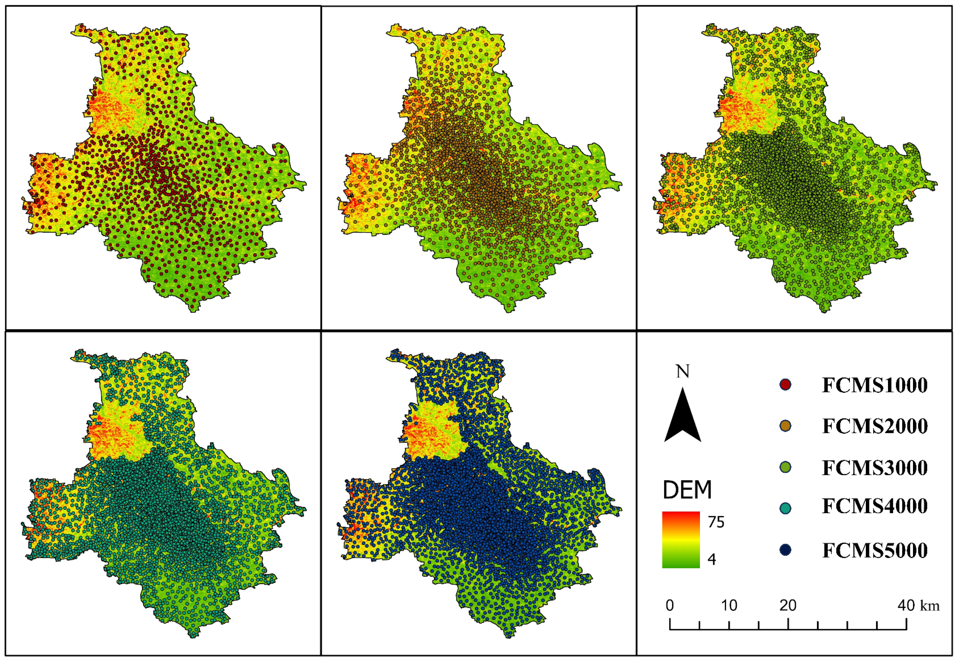
2.3.3. Fuzzy C-Means Clustering Sampling

Fuzzy C-means clustering sampling (FCMS) is a sampling method based on cluster analysis. The membership degree of each sample point to all cluster centers is obtained through optimizing the objective function, thereby determining the class membership of the sample points to achieve automatic classification of the sample data [33]. The sampling points represent the characteristics of each cluster while covering the overall variation range of the soil environment, leading to representativeness and comprehensiveness of sampling [34]. One hundred iterations of model training were performed to optimize and adjust the cluster centers to more accurately reflect the cluster structure of the sample data, and reduce the impact of initial samples on the clustering results, improving clustering stability. This study used Matlab 2018 (MathWorks, USA) to implement FCMS. The steps of the process for FCMS are shown in Table 2, and the sample point sampling results are shown in Figure 4.

2.3.4. Field Calibration

The purpose of field calibration is to verify and assess the accuracy and reliability of maps or data generated by models. By comparing the model’s predicted results with actual field data, field validation can reveal the model’s limitations and errors, providing a basis for subsequent model adjustments and optimizations [35,36]. Representative checkpoints, which reflect the overall variability of soil types, were selected through quick sampling using soil augers or by digging soil profiles. To ensure that the sampling points represent all soil types within Tongzhou District, spatial analysis was conducted on the updated soil type maps in the lab, focusing on the boundaries between different soil types and special topographic areas. Despite the plain nature of Tongzhou District, where surface undulation is minimal, terrain and topography still exert a significant influence on soil formation and distribution. Therefore, special attention was paid to areas where different soil types intersect when planning the validation routes. Additionally, by overlaying the analysis of land-use maps and elevation data, key areas where different soil types might exist were identified, and initial sample points were selected to reflect these characteristics, ensuring comprehensive coverage of soil types across Tongzhou [37,38]. The distribution of the final 97 sample points collected is shown in Figure 5a.

2.4. Random Forest Model

The random forest model (RF) has been widely applied to update conventional soil maps [19,39]. The model predicts soil types by assembling multiple decision trees. It makes full use of the advantages of non-parametric and nonlinear fitting of decision trees. The ensemble of multiple decision trees improves the prediction stability and overcomes the shortcomings of a single decision tree. Compared with traditional soil mapping methods, RF can handle high-dimensional environmental variables, use soil data for effective training, and achieve automatic and accurate prediction of large-scale soil type distributions [40,41,42]. This study implemented the RF model for spatial mapping using R (v4.0.2; R Core Team, 2021).

2.5. Evaluation of Soil Map Accuracy

Soil mapping accuracy is one of the most widely used and important evaluation indicators in machine learning and soil mapping. The overall accuracy of classification or prediction is calculated from the proportion of correctly predicted samples in the classification results [43,44]. The accuracy of the model in classifying soil types is important for model optimization. It is an important evaluation tool to ensure the reliability of soil mapping results. Its principle is shown below [45,46]:
A c c u r a c y = T P + T N T P + F N + F P + T N
where true positives (TP) represent the number of positive examples that are correctly predicted as positive; false negatives (FN) represent the number of positive examples that are incorrectly predicted as negative; false positives (FP) represent the number of negative examples that are incorrectly predicted as positive; true negatives (TN) represent the number of negative examples that are correctly predicted as negative.
Kappa coefficient is a statistical metric widely used to assess the performance of classification models. It takes into account the consistency between the predictions of the model and the actual observations, overcoming the limitation of using only accuracy. The kappa coefficient is calculated using the following formula [47]:
K a p p a = p o p e 1 p e
where p o represents the observed accuracy, and p e represents the accuracy under random classification.
Balanced accuracy is an accuracy metric that takes into account the imbalance in the number of samples in different categories. It calculates the overall accuracy of the model by taking a weighted average of the accuracy of each category. This helps to avoid biased assessment results due to unbalanced sample sizes. The formula for calculating balanced accuracy is as follows [48]:
B a l a n c e d   A c c u r a c y = 1 N i = 1 N T P i T P i + F N i
where N is the number of categories, T P i represents the number of true cases in the ith category, and F N i represents the number of false negative cases in the ith category.

3. Results and Discussion

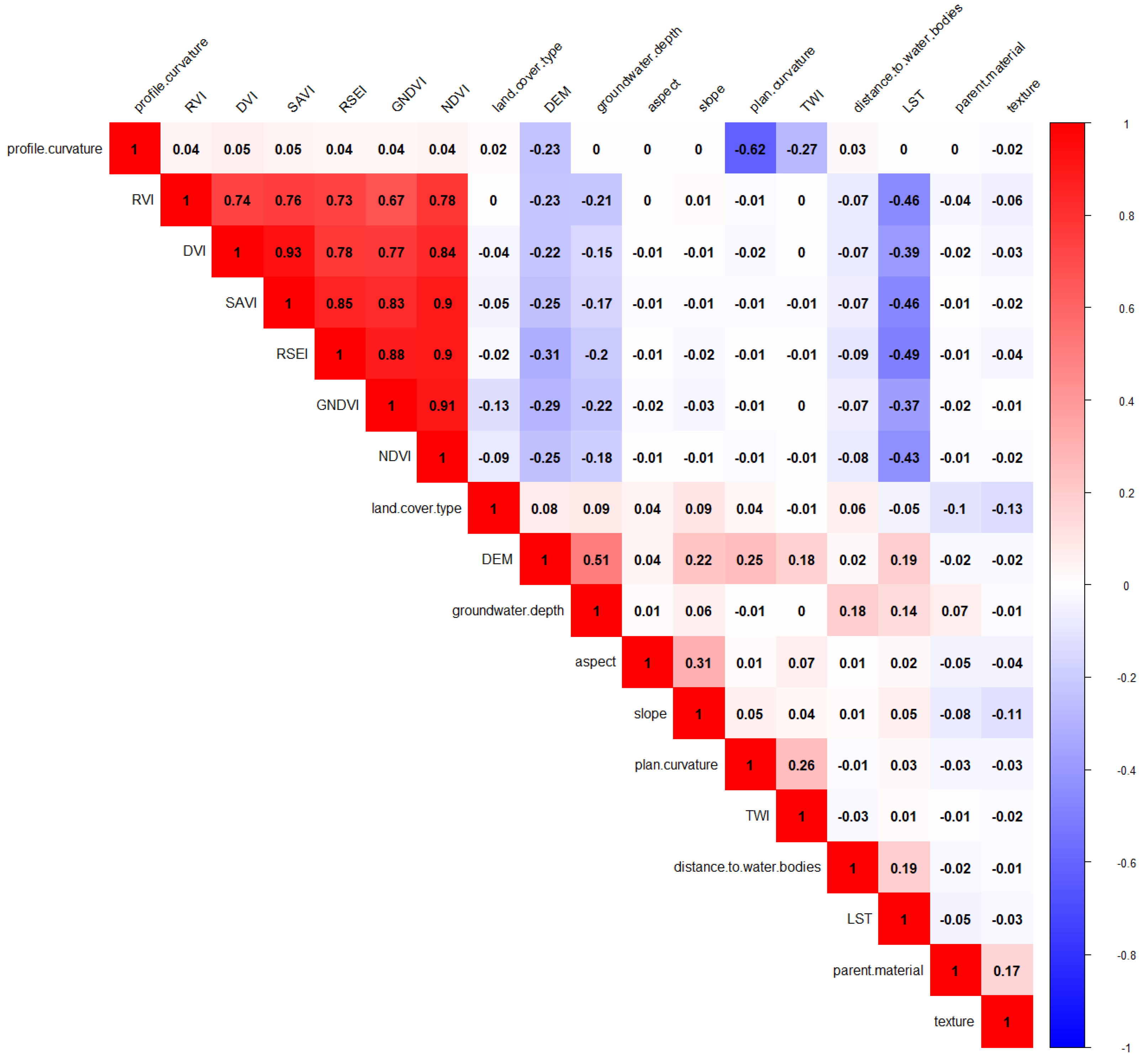
3.1. Selection of Environmental Covariates

This study employs the RF model using the random forest R package to analyze the importance and relevance of environmental covariates in soil mapping, primarily evaluated through the MeanDecreaseAccuracy and MeanDecreaseGini metrics, and further validated using a correlation heatmap. Figure 6 illustrates the importance rankings of various covariates under these two metrics. In Figure 6a, based on the MeanDecreaseAccuracy metric, certain covariates significantly influence the model’s accuracy more than others. For instance, it is evident that LST is the highest-ranked environmental covariate derived from remote sensing data, highlighting its significant role in predicting soil types. As LST captures temperature variations across the landscape, it provides crucial information about soil moisture, thermal properties, and other factors that are essential for distinguishing different soil types. This makes LST a key factor for improving the accuracy of soil type predictions. Figure 6b displays the distribution of covariate importance under the MeanDecreaseGini metric. This metric assesses the decrease in Gini impurity when splitting nodes, revealing the role of covariates in the selection of split points in the decision tree. Some covariates are more prominent under this metric, suggesting they have a higher distinguishing power in differentiating soil types. Through the analysis of Figure 6c, it is found that texture contributes the most to soil mapping, followed by factors such as groundwater depth and distance to water bodies. Figure 7 shows that, due to the study area being a plain region, the contribution of DEM is relatively weak. Meanwhile, there is a strong positive correlation among covariates such as RVI, DVI, SAVI, RSEI, NDVI, and GNDVI, which may lead to multicollinearity issues. Therefore, this study selects RSEI, the covariate with the highest importance, as the representative covariate. Ultimately, groundwater depth, parent material, texture, distance to water bodies, land cover type, elevation, LST, and RSEI were selected as the key environmental covariates used in this study.

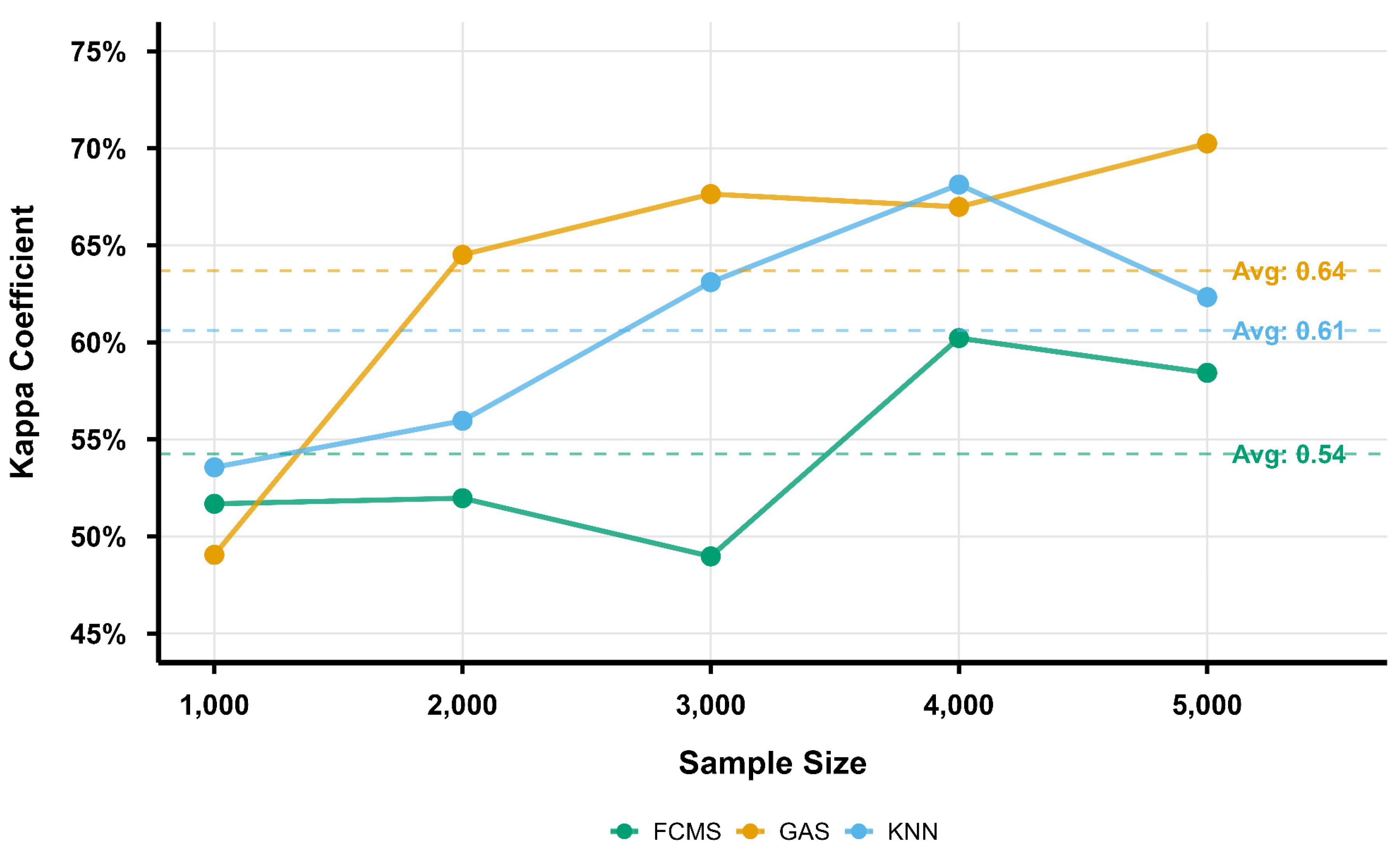
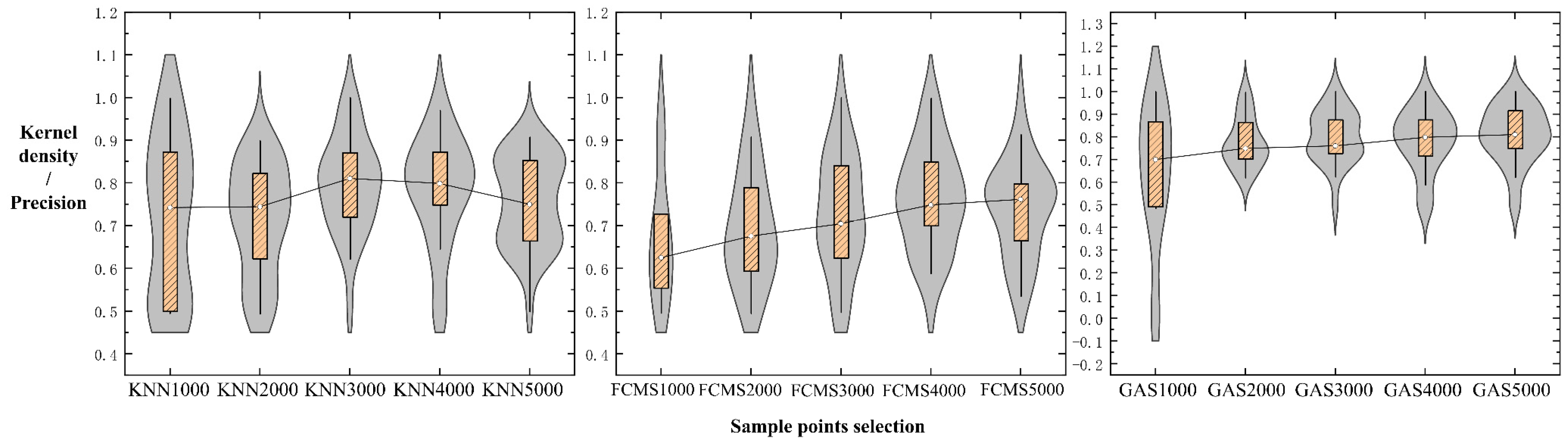
3.2. Comparison of Soil Mapping Accuracy

After applying the RF model uniformly for mapping, as shown in Figure 8, the kappa coefficient of the soil mapping results based on the GAS method increased from 49.05% with 1000 samples to 70.25% with 5000 samples, demonstrating a steady improvement in accuracy as the sample size increased. This indicates that GAS can learn better from larger datasets, exhibiting good scalability. The performance of FCMS showed slight fluctuations with increasing sample size, starting at 51.68%, peaking at 60.22% (with 4000 samples), and then slightly declining to 58.43%. This may suggest that FCMS is more sensitive to changes in sample size, with its performance being significantly affected by the structure of specific sample sets. KNN began at 53.56%, reached its highest accuracy of 68.13% at 4000 samples, and then slightly decreased. The performance trend of KNN indicates that it can effectively utilize larger sample sizes, although the impact of increasing sample size on accuracy diminishes after a certain point. In terms of accuracy changes with sample size, GAS exhibited a sharp increase initially, becoming stable after 2000 samples, and continued to show improvements thereafter, whereas FCMS and KNN demonstrated more fluctuations in performance. Additionally, only GAS ’s kappa value continued to increase after the sample size reached 4000. GAS also showed the highest average accuracy, indicating its overall best performance across different sample sizes. In summary, GAS exhibited the best overall performance, demonstrating high average accuracy and stability.

3.3. Accuracy Range Analysis for Soil Types

As shown in Figure 9, the prediction accuracy of the model for different soil types in Tongzhou District varies under different sampling methods and sample sizes. Under the GAS sampling method, a consistent increase in accuracy is observed as the sample size increases from 1000 to 5000 points. The GAS method shows a marked improvement in accuracy, particularly at higher sample densities, where the accuracy of soil type predictions becomes more concentrated and stable. This trend suggests that GAS is highly effective in capturing the spatial variability of soil attributes, making it a robust choice for updating soil maps in areas with complex soil distributions. In contrast, the KNN method demonstrates relatively stable accuracy across different sample sizes, with minimal fluctuations in the distribution range. However, the accuracy tends to plateau or even decline slightly after reaching a certain sample size, indicating that KNN may have limitations in further improving accuracy with additional sampling. This could be attributed to the method’s reliance on proximity-based classification, which might not fully capture the complexity of soil type variations at higher densities. The FCMS method exhibits a different pattern, where the accuracy distribution shows significant variation across different sample sizes. Notably, the accuracy improves significantly as the sample size increases up to 3000 points, after which the improvement stabilizes. This indicates that while FCMS can effectively enhance accuracy with moderate sample sizes, it may require fine-tuning or additional data to achieve stability and consistency at higher sample densities. In summary, GAS performs the best overall, showing high average accuracy and stability in predicting different soil types.

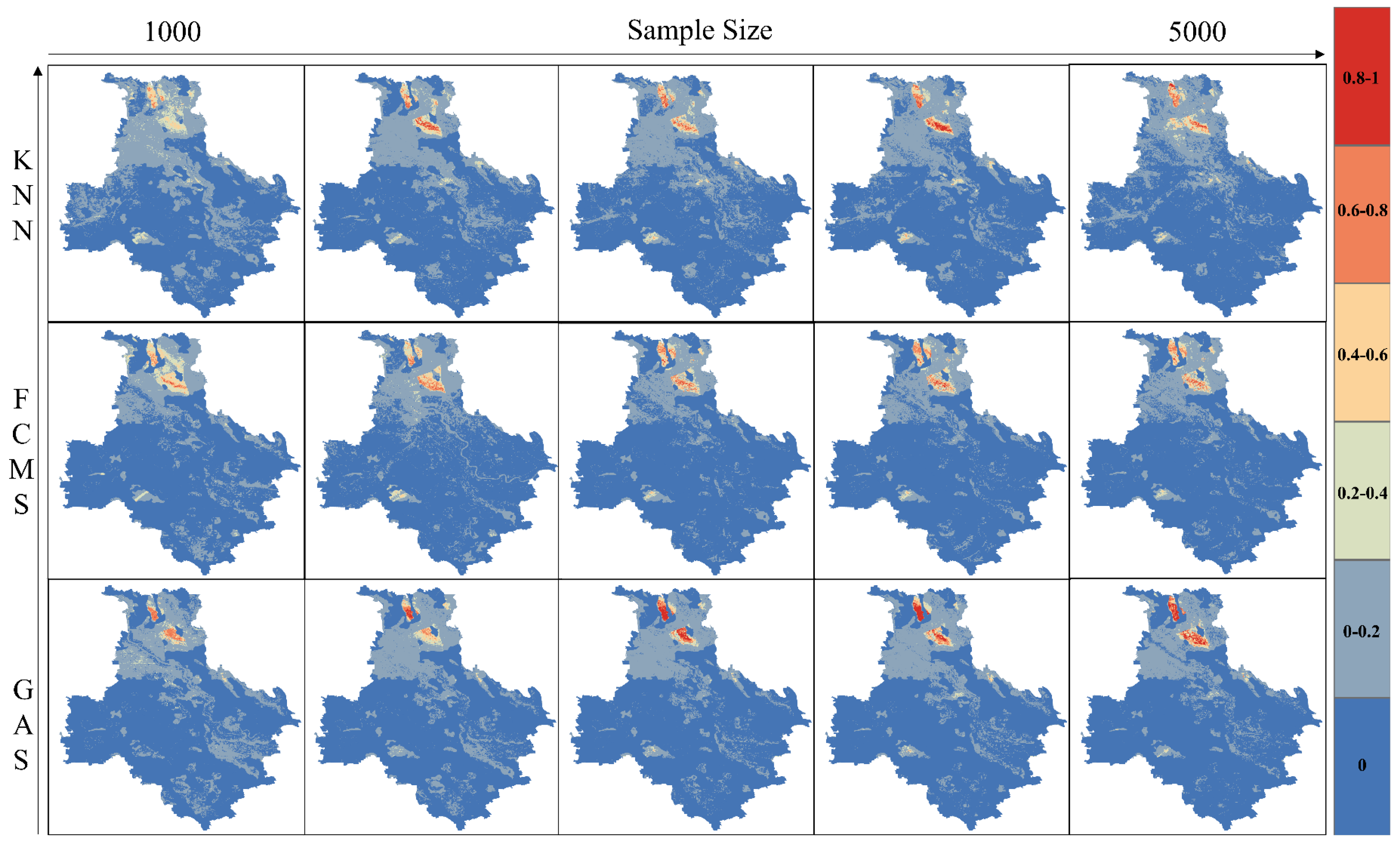
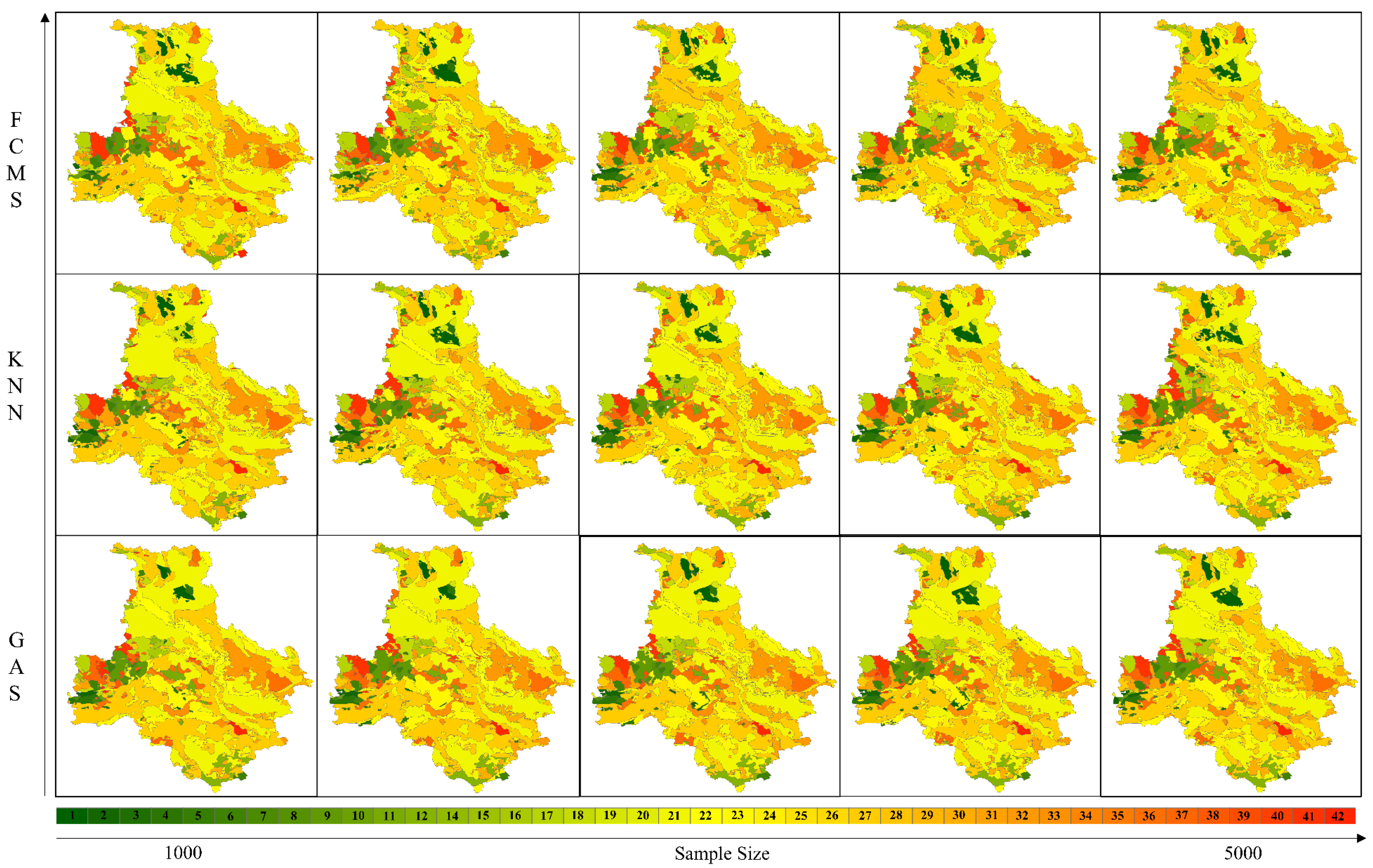
3.4. Comparisons of Mapping Results

As shown in Figure 10, for the KNN method, as the sample size increases, there is a noticeable reduction in uncertainty across the map, particularly when the sample size reaches 5000. The blue regions expand, indicating that the method becomes more reliable in its predictions. However, the remaining red areas suggest that even with larger sample sizes, certain regions remain challenging for the KNN method, reflecting its limitations in fully capturing complex soil variations. The FCMS method shows a less consistent pattern of uncertainty reduction. While an increase in sample size to around 4000 samples does lead to a reduction in uncertainty in some areas, as evidenced by a decrease in red regions, this improvement is not uniform across the entire map. FCMS tends to localize uncertainty reduction, implying that while it can be effective in certain areas, its performance is more variable compared to KNN and GAS. The GAS method, however, shows a complex relationship with uncertainty. Initially, as the sample size increases, there is a significant reduction in uncertainty, similar to the other methods. However, as the sample size reaches 5000, the figure shows an increase in red regions, indicating higher uncertainty. This suggests that while GAS is highly sensitive to changes in sampling size, leading to significant feedback and adjustments in the soil map, it may also introduce higher uncertainty in certain regions at higher sample densities. This sensitivity to sample size makes GAS a powerful tool for soil mapping adjustments, but it also requires careful calibration to avoid increasing uncertainty in certain areas.
Figure 11 shows the soil distribution prediction results under different sample sizes for the three sampling methods (GAS, KNN, FCMS). The GAS method demonstrates high stability across all sample sizes, indicating its ability to maintain consistent predictions of major soil types under different sample sizes, with strong adaptability and global optimization characteristics. This means that GAS can not only capture large-scale soil distribution but also maintain stable prediction performance across different soil types and sampling densities.
In contrast, the KNN method may show significant fluctuations in predicting small, patchy soil types, indicating its greater sensitivity to local variations, though it may be less stable than GAS in handling large-scale, consistent soil types. As can be seen in Figure 2, Figure 3 and Figure 4, the lack of training samples in urban areas leads to weaker model predictions for these areas. There is considerable variation in the results of the FCMS method for different sample sizes, with the predicted values for 1000 samples differing from those for 3000 or more samples, suggesting weak generalization to areas where samples were not deployed. In addition, KNN predicts urban areas differently when the sample size reaches 4000, compared to smaller sample sizes. The GAS method, on the other hand, can effectively simulate the spatial distribution pattern of major soil types in the region by using its global optimization capability and shows strong adaptability and stable prediction performance under different soil types and sampling densities.

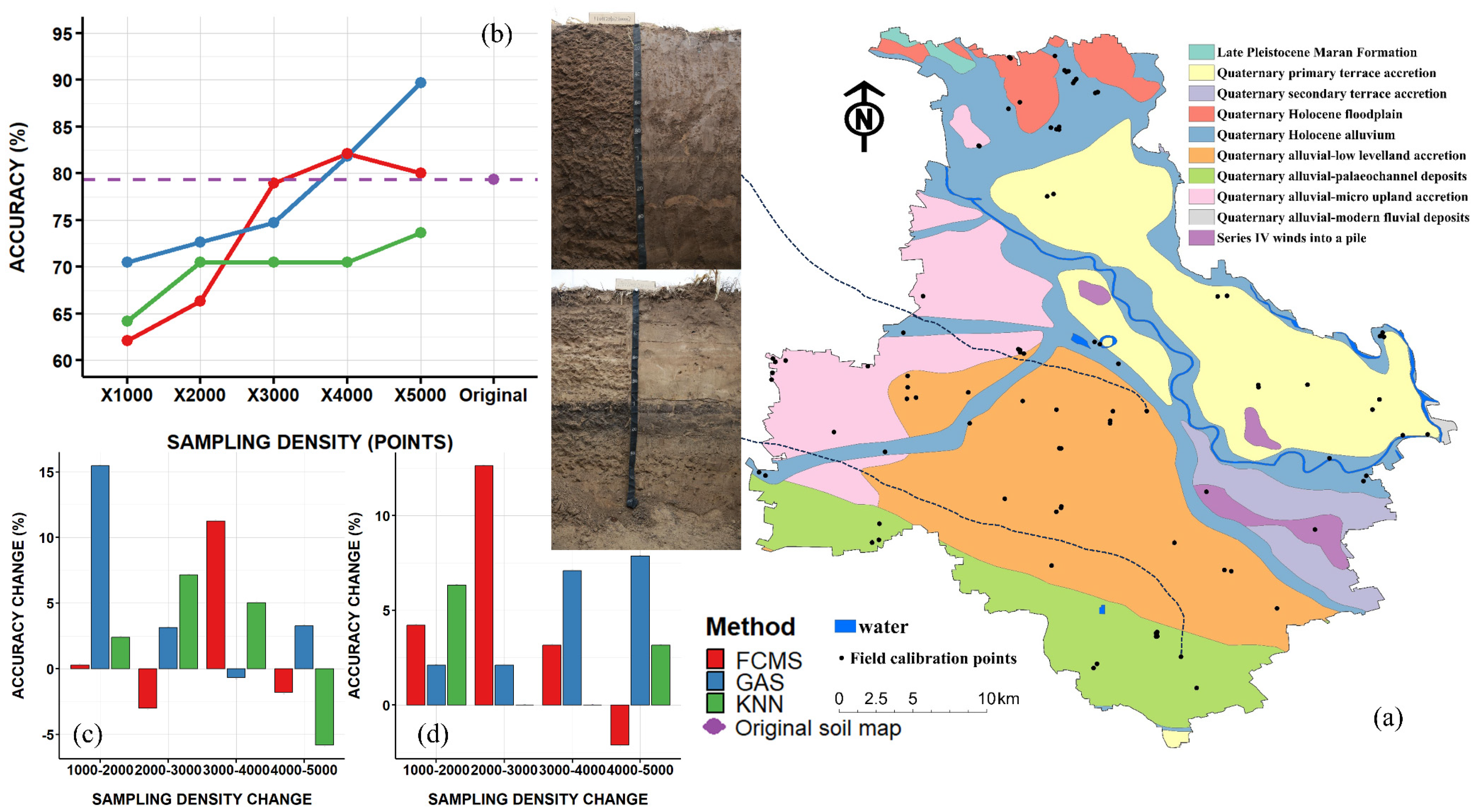
3.5. Status of Field Calibration

In this study, the accuracy variation of different models across various sampling densities was systematically analyzed, and the effectiveness of these models was validated through field verification. As shown in Figure 5b, the GAS model exhibited a significant improvement in accuracy as the sampling density increased, reaching 89.69% accuracy at 5000 sample points, which is notably higher than that of the KNN and FCMS models. Additionally, the GAS model’s accuracy surpassed that of the original soil map, indicating its stronger mapping capabilities at higher sampling densities, whereas the field-verified accuracy of other models only slightly exceeded or fell below that of the original soil map. Figure 5c,d further illustrate the trends in model accuracy and field-verified accuracy. It was observed that between 1000 and 2000 sample points, the GAS model demonstrated the greatest improvement in accuracy, indicating that increasing the number of sample points is crucial for enhancing the mapping accuracy of the GAS model. Moreover, the FCMS model exhibited a notable improvement in accuracy in the 2000 to 3000 sample point range, suggesting that this model can significantly improve mapping accuracy with a moderate increase in sample points. However, it is worth noting that although the KNN model remained relatively stable at low-density sample points, its accuracy improvement was relatively minor at higher-density sample points. By comparing the field-verified results with the model accuracy changes, it is evident that the GAS model exhibits excellent adaptability and accuracy at high sampling densities.

3.6. Discussions for Sampling Algorithm Differences

The performance differences among sampling algorithms primarily stem from their ability to utilize environmental covariate information and optimize sampling point layouts [49]. KNN and FCMS have limitations in leveraging environmental covariate data, particularly in plain areas, where the terrain is uniform, and spatial variability is low [50]. In such scenarios, these methods struggle to fully capture soil spatial heterogeneity, resulting in reduced mapping accuracy [35]. Specifically, the KNN method selects sampling points based on the nearest neighbor relationships of environmental covariates [43]. However, it lacks the capability to dynamically adjust the distribution of sampling points, often concentrating samples in areas with uniform covariate distributions while neglecting regions with significant local variations [51]. Similarly, the FCMS method generates sampling points based on clustering results of environmental covariates [52]. When covariate characteristics are relatively homogeneous, sampling points tend to cluster within a few groups, failing to comprehensively cover the spatial distribution of soil attributes [53]. Additionally, neither of these methods can effectively incorporate the expert knowledge embedded in legacy soil maps, such as soil type boundaries and prior soil–environment relationships.
In contrast, the GAS method demonstrates significant advantages in integrating legacy soil maps with environmental covariate information [13]. The GAS method iteratively optimizes the fitness function, considering both the spatial heterogeneity of environmental covariates and the soil type distribution characteristics captured in legacy soil maps. This enables GAS to intelligently adjust the sampling point layout, aligning it more closely with the actual soil spatial variability [54]. In plain areas, GAS effectively mitigates issues arising from low spatial variability, ensuring a more balanced distribution of sampling points [55]. Moreover, GAS emphasizes sampling in key regions, such as soil type boundaries and transition zones, significantly improving mapping accuracy and stability [45]. Through multiple iterations, the GAS method dynamically adjusts the sampling point layout, enhancing sample representativeness and capturing complex soil–environment relationships [56]. At the same time, the selection of environmental covariates is crucial, as different covariates have varying abilities to capture soil spatial variability, which directly impacts the effectiveness of the sampling points obtained by different algorithms [57]. In future studies, it may be beneficial to consider data related to soil depth and diagnostic horizons when selecting environmental covariates [58]. Soil depth directly influences root development, water retention, and nutrient availability, making it a key indicator for distinguishing soil types. Diagnostic horizons are fundamental to soil taxonomy, effectively reflecting pedogenic processes and spatial differentiation. Both of these factors can provide more accurate supporting information for sampling point collection and model prediction.

3.7. Improving the Utilization of Soil Resources in Agriculture

This study classified regional soils using soil type maps, analyzed soil distribution, properties and suitability, and provided support for agricultural management and decision-making. Soil resources were divided into five grades and ten types, and corresponding improvement and utilization measures were proposed for different types. See the Supplementary Materials for details.

4. Conclusions

By comparing GAS with two other sampling methods, KNN and FCMS, under the RF model, the results demonstrated that GAS consistently outperformed the other methods in terms of accuracy, stability, and adaptability. The key findings can be summarized as follows:
Superior accuracy: The GAS method exhibited higher accuracy across various sample sizes compared to KNN and FCMS. The kappa coefficient of the soil mapping results showed a significant improvement with the increase in sample size, reaching 70.25% at 5000 samples. GAS maintained high accuracy and showed better scalability as the sample size increased.
Stability and consistency: GAS demonstrated more stable performance, with minimal fluctuations in accuracy across different sample sizes. This stability is crucial for ensuring reliable soil mapping, particularly in areas with uniform topography and minimal variability in soil attributes.
Field validation: The field validation results confirmed the superiority of GAS, with a notable accuracy of 89.69% at 5000 sample points. This accuracy was significantly higher than that of KNN and FCMS, underscoring the effectiveness of GAS in practical applications.
Soil resources play a crucial role in agricultural production, as they directly affect crop growth and yield. The improvement and sustainable utilization of soil are essential for enhancing agricultural productivity and ensuring long-term food security. It is necessary to develop more advanced and environmentally friendly methods to obtain more accurate information on the distribution of soil types in order to optimize soil use, reduce the negative effects of overuse, and promote sustainable agricultural practices.

Supplementary Materials

The following supporting information can be downloaded at: https://www.mdpi.com/article/10.3390/agronomy15040963/s1, Table S1: Soil Types In Tongzhou District; Table S2: Statistical tables for soil resource assessment.

Author Contributions

Conceptualization, X.W. and Y.L.; methodology, X.W.; software, K.W.; validation, Y.L., K.W. and S.H; formal analysis, X.W.; investigation, X.W.; resources, K.W.; data curation, S.H; writing—original draft preparation, X.W.; writing—review and editing, Y.L.; visualization, K.W.; supervision, Y.L.; project administration, S.H.; funding acquisition, Y.L. All authors have read and agreed to the published version of the manuscript.

Funding

This research was funded by the Humanities and Social Science Foundation of the Ministry of Education of China (22YJAZH055), the National Natural Science Foundation of China (Grants No. 42271261), and the Fundamental Research Funds for the Central Universities.

Data Availability Statement

The original contributions presented in the study are included in the article/Supplementary Material, further inquiries can be directed to the corresponding author.

Conflicts of Interest

The authors declare no conflicts of interest.

References

  1. Sulaeman, Y.; Minasny, B.; McBratney, A.B.; Sarwani, M.; Sutandi, A. Harmonizing Legacy Soil Data for Digital Soil Mapping in Indonesia. Geoderma 2013, 192, 77–85. [Google Scholar] [CrossRef]
  2. Zeraatpisheh, M.; Bakhshandeh, E.; Hosseini, M.; Alavi, S.M. Assessing the Effects of Deforestation and Intensive Agriculture on the Soil Quality through Digital Soil Mapping. Geoderma 2020, 363, 114139. [Google Scholar] [CrossRef]
  3. Chen, S.; Arrouays, D.; Leatitia Mulder, V.; Poggio, L.; Minasny, B.; Roudier, P.; Libohova, Z.; Lagacherie, P.; Shi, Z.; Hannam, J.; et al. Digital Mapping of GlobalSoilMap Soil Properties at a Broad Scale: A Review. Geoderma 2022, 409, 115567. [Google Scholar] [CrossRef]
  4. Petrovskaia, A.; Ryzhakov, G.; Oseledets, I. Optimal Soil Sampling Design Based on the Maxvol Algorithm. Geoderma 2021, 402, 115362. [Google Scholar] [CrossRef]
  5. Yang, L.; Brus, D.J.; Zhu, A.-X.; Li, X.; Shi, J. Accounting for Access Costs in Validation of Soil Maps: A Comparison of Design-Based Sampling Strategies. Geoderma 2018, 315, 160–169. [Google Scholar] [CrossRef]
  6. Brus, D.J. Balanced Sampling: A Versatile Sampling Approach for Statistical Soil Surveys. Geoderma 2015, 253–254, 111–121. [Google Scholar] [CrossRef]
  7. Krumbein, W.C. Factors of Soil Formation: A System of Quantitative Pedology. Hans Jenny. J. Geol. 1942, 50, 919–920. [Google Scholar] [CrossRef]
  8. Minasny, B.; McBratney, A.B. Digital Soil Mapping: A Brief History and Some Lessons. Geoderma 2016, 264, 301–311. [Google Scholar] [CrossRef]
  9. Yang, L.; Li, X.; Shi, J.; Shen, F.; Qi, F.; Gao, B.; Chen, Z.; Zhu, A.-X.; Zhou, C. Evaluation of Conditioned Latin Hypercube Sampling for Soil Mapping Based on a Machine Learning Method. Geoderma 2020, 369, 114337. [Google Scholar] [CrossRef]
  10. Stumpf, F.; Schmidt, K.; Behrens, T.; Schönbrodt-Stitt, S.; Buzzo, G.; Dumperth, C.; Wadoux, A.; Xiang, W.; Scholten, T. Incorporating Limited Field Operability and Legacy Soil Samples in a Hypercube Sampling Design for Digital Soil Mapping. J. Plant Nutr. Soil Sci. 2016, 179, 499–509. [Google Scholar] [CrossRef]
  11. Zhu, A.X.; Yang, L.; Li, B.; Qin, C.; English, E.; Burt, J.E.; Zhou, C. Purposive Sampling for Digital Soil Mapping for Areas with Limited Data. In Digital Soil Mapping with Limited Data; Hartemink, A.E., McBratney, A., Mendonça-Santos, M.d.L., Eds.; Springer: Dordrecht, The Netherland, 2008; pp. 233–245. [Google Scholar]
  12. Barthold, F.K.; Wiesmeier, M.; Breuer, L.; Frede, H.-G.; Wu, J.; Blank, F.B. Land Use and Climate Control the Spatial Distribution of Soil Types in the Grasslands of Inner Mongolia. J. Arid Environ. 2013, 88, 194–205. [Google Scholar] [CrossRef]
  13. Wadoux, A.M.J.-C.; Brus, D.J.; Heuvelink, G.B.M. Sampling Design Optimization for Soil Mapping with Random Forest. Geoderma 2019, 355, 113913. [Google Scholar] [CrossRef]
  14. Kempen, B.; Brus, D.J.; Heuvelink, G.B.M.; Stoorvogel, J.J. Updating the 1:50,000 Dutch Soil Map Using Legacy Soil Data: A Multinomial Logistic Regression Approach. Geoderma 2009, 151, 311–326. [Google Scholar] [CrossRef]
  15. Zeng, C.; Qi, F.; Zhu, A.-X.; Liu, F. Construction of Land Surface Dynamic Feedback for Digital Soil Mapping Considering the Spatial Heterogeneity of Rainfall Magnitude. CATENA 2020, 191, 104576. [Google Scholar] [CrossRef]
  16. Deb, K. Multi-Objective Optimisation Using Evolutionary Algorithms: An Introduction. In Multi-Objective Evolutionary Optimisation for Product Design and Manufacturing; Wang, L., Ng, A.H.C., Deb, K., Eds.; Springer: London, UK, 2011; pp. 3–34. [Google Scholar]
  17. Goldberg, D.E.; Holland, J.H. Genetic Algorithms and Machine Learning. Mach. Learn. 1988, 3, 95–99. [Google Scholar] [CrossRef]
  18. The Third National Soil Survey Work Plan. Available online: https://www.gov.cn/xinwen/2022-02/24/content_5675442.htm (accessed on 8 April 2024).
  19. Heung, B.; Ho, H.C.; Zhang, J.; Knudby, A.; Bulmer, C.E.; Schmidt, M.G. An Overview and Comparison of Machine-Learning Techniques for Classification Purposes in Digital Soil Mapping. Geoderma 2016, 265, 62–77. [Google Scholar] [CrossRef]
  20. Xu, Y.; Li, K.; Hu, J.; Li, K. A Genetic Algorithm for Task Scheduling on Heterogeneous Computing Systems Using Multiple Priority Queues. Inf. Sci. 2014, 270, 255–287. [Google Scholar] [CrossRef]
  21. Sun, Y.; Xue, B.; Zhang, M.; Yen, G.G.; Lv, J. Automatically Designing CNN Architectures Using the Genetic Algorithm for Image Classification. IEEE Trans. Cybern. 2020, 50, 3840–3854. [Google Scholar] [CrossRef]
  22. Soleimani, H.; Kannan, G. A Hybrid Particle Swarm Optimization and Genetic Algorithm for Closed-Loop Supply Chain Network Design in Large-Scale Networks. Appl. Math. Model. 2015, 39, 3990–4012. [Google Scholar] [CrossRef]
  23. Deng, W.; Zhao, H.; Zou, L.; Li, G.; Yang, X.; Wu, D. A Novel Collaborative Optimization Algorithm in Solving Complex Optimization Problems. Soft Comput. 2017, 21, 4387–4398. [Google Scholar] [CrossRef]
  24. Mumali, F.; Kałkowska, J. Intelligent Support in Manufacturing Process Selection Based on Artificial Neural Networks, Fuzzy Logic, and Genetic Algorithms: Current State and Future Perspectives. Comput. Ind. Eng. 2024, 193, 110272. [Google Scholar] [CrossRef]
  25. Borcard, D.; Gillet, F.; Legendre, P. Numerical Ecology with R; Use R! Springer International Publishing: Cham, Switzerland, 2018; ISBN 978-3-319-71403-5. [Google Scholar]
  26. Sánchez-Mercado, A.Y.; Ferrer-Paris, J.R.; Franklin, J. Mapping Species Distributions: Spatial Inference and Prediction. Oryx 2010, 44, 615. [Google Scholar] [CrossRef]
  27. Guisan, A.; Zimmermann, N.E. Predictive Habitat Distribution Models in Ecology. Ecol. Model. 2000, 135, 147–186. [Google Scholar] [CrossRef]
  28. Hijmans, R.J.; Cameron, S.E.; Parra, J.L.; Jones, P.G.; Jarvis, A. Very High Resolution Interpolated Climate Surfaces for Global Land Areas. Int. J. Climatol. 2005, 25, 1965–1978. [Google Scholar] [CrossRef]
  29. Rogers, D.J.; Randolph, S.E. Studying the Global Distribution of Infectious Diseases Using GIS and RS. Nat. Rev. Microbiol. 2003, 1, 231–237. [Google Scholar] [CrossRef] [PubMed]
  30. Rosenberg, M.S.; Anderson, C.D. PASSaGE: Pattern Analysis, Spatial Statistics and Geographic Exegesis. Version 2. Methods Ecol. Evol. 2011, 2, 229–232. [Google Scholar] [CrossRef]
  31. Luo, X.; Wang, H.; Wu, D.; Chen, C.; Deng, M.; Huang, J.; Hua, X.-S. A Survey on Deep Hashing Methods. ACM Trans. Knowl. Discov. Data 2023, 17, 1–50. [Google Scholar] [CrossRef]
  32. Li, J.; Lin, S.; Yu, K.; Guo, G. Quantum K-Nearest Neighbor Classification Algorithm Based on Hamming Distance. Quantum Inf. Process 2021, 21, 18. [Google Scholar] [CrossRef]
  33. Mohammadrezapour, O.; Kisi, O.; Pourahmad, F. Fuzzy C-Means and K-Means Clustering with Genetic Algorithm for Identification of Homogeneous Regions of Groundwater Quality. Neural Comput. Applic 2020, 32, 3763–3775. [Google Scholar] [CrossRef]
  34. Horta, A.; Malone, B.; Stockmann, U.; Minasny, B.; Bishop, T.F.A.; McBratney, A.B.; Pallasser, R.; Pozza, L. Potential of Integrated Field Spectroscopy and Spatial Analysis for Enhanced Assessment of Soil Contamination: A Prospective Review. Geoderma 2015, 241–242, 180–209. [Google Scholar] [CrossRef]
  35. Minasny, B.; McBratney, A.B. A Conditioned Latin Hypercube Method for Sampling in the Presence of Ancillary Information. Comput. Geosci. 2006, 32, 1378–1388. [Google Scholar] [CrossRef]
  36. Hengl, T.; Heuvelink, G.B.M.; Stein, A. A Generic Framework for Spatial Prediction of Soil Variables Based on Regression-Kriging. Geoderma 2004, 120, 75–93. [Google Scholar] [CrossRef]
  37. Zhu, A.X.; Hudson, B.; Burt, J.; Lubich, K.; Simonson, D. Soil Mapping Using GIS, Expert Knowledge, and Fuzzy Logic. Soil. Sci. Soc. Am. J. 2001, 65, 1463–1472. [Google Scholar] [CrossRef]
  38. Mulder, V.L.; de Bruin, S.; Schaepman, M.E.; Mayr, T.R. The Use of Remote Sensing in Soil and Terrain Mapping—A Review. Geoderma 2011, 162, 1–19. [Google Scholar] [CrossRef]
  39. Guo, P.-T.; Li, M.-F.; Luo, W.; Tang, Q.-F.; Liu, Z.-W.; Lin, Z.-M. Digital Mapping of Soil Organic Matter for Rubber Plantation at Regional Scale: An Application of Random Forest plus Residuals Kriging Approach. Geoderma 2015, 237–238, 49–59. [Google Scholar] [CrossRef]
  40. Chen, W.; Xie, X.; Wang, J.; Pradhan, B.; Hong, H.; Bui, D.T.; Duan, Z.; Ma, J. A Comparative Study of Logistic Model Tree, Random Forest, and Classification and Regression Tree Models for Spatial Prediction of Landslide Susceptibility. CATENA 2017, 151, 147–160. [Google Scholar] [CrossRef]
  41. Brungard, C.W.; Boettinger, J.L.; Duniway, M.C.; Wills, S.A.; Edwards, T.C. Machine Learning for Predicting Soil Classes in Three Semi-Arid Landscapes. Geoderma 2015, 239–240, 68–83. [Google Scholar] [CrossRef]
  42. Breiman, L. Random Forests. Mach. Learn. 2001, 45, 5–32. [Google Scholar] [CrossRef]
  43. Were, K.; Bui, D.T.; Dick, Ø.B.; Singh, B.R. A Comparative Assessment of Support Vector Regression, Artificial Neural Networks, and Random Forests for Predicting and Mapping Soil Organic Carbon Stocks across an Afromontane Landscape. Ecol. Indic. 2015, 52, 394–403. [Google Scholar] [CrossRef]
  44. Schmidt, K.; Behrens, T.; Scholten, T. Instance Selection and Classification Tree Analysis for Large Spatial Datasets in Digital Soil Mapping. Geoderma 2008, 146, 138–146. [Google Scholar] [CrossRef]
  45. Keskin, H.; Grunwald, S.; Harris, W.G. Digital Mapping of Soil Carbon Fractions with Machine Learning. Geoderma 2019, 339, 40–58. [Google Scholar] [CrossRef]
  46. Stum, A.K.; Boettinger, J.L.; White, M.A.; Ramsey, R.D. Random Forests Applied as a Soil Spatial Predictive Model in Arid Utah. In Digital Soil Mapping: Bridging Research, Environmental Application, and Operation; Boettinger, J.L., Howell, D.W., Moore, A.C., Hartemink, A.E., Kienast-Brown, S., Eds.; Springer: Dordrecht, The Netherland, 2010; pp. 179–190. [Google Scholar]
  47. Cohen, J. A Coefficient of Agreement for Nominal Scales. Educ. Psychol. Meas. 1960, 20, 37–46. [Google Scholar] [CrossRef]
  48. Tharwat, A. Classification Assessment Methods. Appl. Comput. Inform. 2021, 17, 168–192. [Google Scholar] [CrossRef]
  49. Brus, D.J. Sampling for Digital Soil Mapping: A Tutorial Supported by R Scripts. Geoderma 2019, 338, 464–480. [Google Scholar] [CrossRef]
  50. Hengl, T.; Nussbaum, M.; Wright, M.N.; Heuvelink, G.B.M.; Gräler, B. Random Forest as a Generic Framework for Predictive Modeling of Spatial and Spatio-Temporal Variables. PeerJ 2018, 6, e5518. [Google Scholar] [CrossRef] [PubMed]
  51. Li, J.; Heap, A.D.; Potter, A.; Daniell, J.J. Application of Machine Learning Methods to Spatial Interpolation of Environmental Variables. Environ. Model. Softw. 2011, 26, 1647–1659. [Google Scholar] [CrossRef]
  52. Lagacherie, P.; Arrouays, D.; Bourennane, H.; Gomez, C.; Martin, M.; Saby, N.P.A. How Far Can the Uncertainty on a Digital Soil Map Be Known?: A Numerical Experiment Using Pseudo Values of Clay Content Obtained from Vis-SWIR Hyperspectral Imagery. Geoderma 2019, 337, 1320–1328. [Google Scholar] [CrossRef]
  53. Arrouays, D.; Leenaars, J.G.B.; Richer-de-Forges, A.C.; Adhikari, K.; Ballabio, C.; Greve, M.; Grundy, M.; Guerrero, E.; Hempel, J.; Hengl, T.; et al. Soil Legacy Data Rescue via GlobalSoilMap and Other International and National Initiatives. GeoResJ 2017, 14, 1–19. [Google Scholar] [CrossRef]
  54. Caubet, M.; Román Dobarco, M.; Arrouays, D.; Minasny, B.; Saby, N.P.A. Merging Country, Continental and Global Predictions of Soil Texture: Lessons from Ensemble Modelling in France. Geoderma 2019, 337, 99–110. [Google Scholar] [CrossRef]
  55. Piikki, K.; Söderström, M.; Stadig, H. Local Adaptation of a National Digital Soil Map for Use in Precision Agriculture. Adv. Anim. Biosci. 2017, 8, 430–432. [Google Scholar] [CrossRef]
  56. Padarian, J.; Minasny, B.; McBratney, A.B. Machine Learning and Soil Sciences: A Review Aided by Machine Learning Tools. SOIL 2020, 6, 35–52. [Google Scholar] [CrossRef]
  57. Li, X.; Gu, H.; Tang, R.; Zou, B.; Liu, X.; Ou, H.; Chen, X.; Song, Y.; Luo, W.; Wen, B. A Fusion XGBoost Approach for Large-Scale Monitoring of Soil Heavy Metal in Farmland Using Hyperspectral Imagery. Agronomy 2025, 15, 676. [Google Scholar] [CrossRef]
  58. Li, Y.; Yao, G.; Li, S.; Dong, X. Predicting and Mapping of Soil Organic Matter with Machine Learning in the Black Soil Region of the Southern Northeast Plain of China. Agronomy 2025, 15, 533. [Google Scholar] [CrossRef]
Figure 1. Map of original soil types in the study area. Table S1 in the Supplementary Material lists the specific meanings of the codes shown in the figure, providing explanations of the correspondence between soil type codes and their respective soil type names. Number “13” was missing because the soil type it represents covers a very small area and did not meet the size requirement needed for display.
Agronomy 15 00963 g001
Figure 2. Spatial distribution of sampling points selected by the GAS method under different sample sizes (1000–5000 points) in Tongzhou District, Beijing.
Agronomy 15 00963 g002
Figure 3. Spatial distribution of sampling points selected by the KNN method under different sample sizes (1000–5000 points) in Tongzhou District, Beijing.
Agronomy 15 00963 g003
Figure 4. Spatial distribution of sampling points selected by the FCMS method under different sample sizes (1000–5000 points) in Tongzhou District, Beijing.
Agronomy 15 00963 g004
Figure 5. Field calibration results. (a) Distribution of field calibrated sample points, with two sample points used for digging typical soil profiles. (b) Actual prediction accuracy of different sampling models during field calibration under various sample sizes. (c) Trends in model accuracy for each method as sample density changes. (d) Trends in field calibration accuracy for each method across different sample size intervals.
Agronomy 15 00963 g005
Figure 6. Importance of environmental covariates based on different evaluation metrics. (a) MeanDecreaseAccuracy: Shows the reduction in model prediction accuracy when each covariate is excluded. A larger value indicates greater importance. (b) MeanDecreaseGini: Reflects the total decrease in node impurity when the covariate is used for splitting; higher values suggest higher relevance for classification. (c) Overall importance ranking of covariates based on normalized values. Darker blue bars represent higher importance, while lighter blue bars indicate lower contribution.
Agronomy 15 00963 g006
Figure 7. Correlation of environmental covariates. The color scale represents the strength and direction of the correlation, with red indicating a strong positive correlation, blue indicating a strong negative correlation, and white indicating no correlation.
Agronomy 15 00963 g007
Figure 8. Kappa coefficient of soil maps with different sample selections.
Agronomy 15 00963 g008
Figure 9. Distribution of balanced accuracy across different sampling selections for KNN, FCMS, and GAS methods, calculated for all soil types in Tongzhou District. Each violin plot represents the kernel density distribution, with the orange box in the middle indicating the median of the balanced accuracy. The left, middle, and right plots correspond to the performance of the KNN, FCMS, and GAS methods under different sample sizes, respectively.
Agronomy 15 00963 g009
Figure 10. Uncertainty map of RF predictions for different sampling sizes and methods. The color scale represents the level of uncertainty, with blue indicating low uncertainty and red indicating high uncertainty.
Agronomy 15 00963 g010
Figure 11. Predicted soil distribution map. The numbers in the legend correspond to the soil codes listed in Table S1 of the Supplementary Material, representing the respective soil types.
Agronomy 15 00963 g011
Table 1. Selected environmental covariates.
No.NameAbbreviationResolutionSource
1Parent Material-1:25,000Digitized geological map of China
2Texture--Indoor calibration soil map
3Land Cover Type-30 mGlobeLand30
4ElevationDEM12.5 mNational Science & Technology Infrastructure of China (http://www.geodata.cn)
5Slope-Derived from DEMProcessed using ArcGIS
6Aspect-Derived from DEMProcessed using ArcGIS
7Planar Curvature-Derived from DEMProcessed using ArcGIS
8Profile Curvature-Derived from DEMProcessed using ArcGIS
9Topographic Wetness IndexTWIDerived from DEMProcessed using ArcGIS
10Distance to water bodies--Processed using ArcGIS and water system data
11Groundwater Depth--Water Affairs Bureau of Tongzhou District, interpolated using inverse distance weighting
12Risk-Screening Environmental IndicatorsRSEI30 mLandsat imagery processed using Google Earth Engine
13Land Surface TemperatureLST30 mLandsat imagery processed using Google Earth Engine
14Soil-Adjusted Vegetation IndexSAVI30 mLandsat imagery processed using Google Earth Engine
15Normalized Difference Vegetation IndexNDVI30 mLandsat imagery processed using Google Earth Engine
16Difference Vegetation IndexDVI30 mLandsat imagery processed using Google Earth Engine
17Ratio Vegetation IndexRVI30 mLandsat imagery processed using Google Earth Engine
18Green Normalized Difference Vegetation IndexGNDVI30 mLandsat imagery processed using Google Earth Engine
Table 2. Construction steps for FCMS.
StepDescription
1Overlay the environmental variable dataset in space.
2Perform FCM clustering analysis on the data and divide the data into multiple classes.
3Iterate to optimize the cluster centers, train 100 times.
4Randomly select sampling points within each optimized class.
5Repeat step 4 until the number of sampling points reaches the required amount.
Disclaimer/Publisher’s Note: The statements, opinions and data contained in all publications are solely those of the individual author(s) and contributor(s) and not of MDPI and/or the editor(s). MDPI and/or the editor(s) disclaim responsibility for any injury to people or property resulting from any ideas, methods, instructions or products referred to in the content.

