Performance Analysis of Real-Time Detection Transformer and You Only Look Once Models for Weed Detection in Maize Cultivation

Abstract

Weeds are unwanted and invasive plants characterized by their rapid growth and ability to compete with crops for essential resources such as space, water, nutrients, and sunlight. This competition has a negative impact on crop quality and productivity. To reduce the influence of weeds, precision weeding is used, which uses image sensors and computational algorithms to identify plants and classify weeds using digital images. This study used images of maize (Zea mays L.) to detect four types of weeds (Lolium rigidum, Sonchus oleraceus, Solanum nigrum, and Poa annua). For this purpose, YOLO (You Only Look Once) architectures, YOLOv8s, YOLOv9s, YOLOv10s, and YOLOv11s versions, were trained and compared, along with an architecture based on RT-DETR (Real-Time Detection Transformer), version RT-DETR-1. The YOLO architectures are noted for their real-time detection efficiency, and RT-DETR-l allows evaluation of the impact of an architecture that dispenses with Non-Maximum Suppression (NMS). The YOLOv9s model had the best overall performance, achieving a mAP@0.5 of 0.834 in 60 epochs and an F1-score of 0.78, which demonstrates a optimal balance between accuracy and recall, although with less confidence in its predictions. On the other hand, the RT-DETR-l model stood out for its efficiency in convergence, reaching a competitive performance in only 58 epochs with a mAP@0.5 of 0.828 and an F1-score of 0.80.

1. Introduction

Corn (Zea mays L.) is the main cereal planted in the world, reaching a production of 1.16 billion tons in 2022 [1]. Maize is intended for human consumption and is a key input for various industries and animal feed. Therefore, to ensure corn productivity, it is essential to strengthen agronomic management plans, especially integrated weed management, which is crucial to maintaining high production levels [2]. Moreover, weeds are fast-growing plants that compete with crops for resources such as space, water, nutrients, and sunlight. This competition negatively affects both crop yield and crop quality [3]. According to the study in [4], the presence of weeds can cause losses of up to 42% in agricultural production. Several eradication methods are used to control weeds; the most used is the application of herbicides before or after weed emergence, which not only generates negative environmental impacts but also affects workers’ health [5]. Another traditional method for weed control is mechanical weeding, which can be carried out using machines or manually. However, its cost is higher compared to the application of herbicides. This has driven the search for alternatives based on the adoption of new technologies, aiming to improve the process’s efficiency and make it economically viable while minimizing environmental impacts.

In recent years, the rapid evolution of Artificial Intelligence (AI) has transformed the primary sector, driving the use of technologies such as machine learning (ML), computer vision, and robotics, which enable the capture and analysis of large volumes of data, facilitating decision-making [6]. Their application, in combination with AI techniques, has been implemented in various areas of food production, including animal production [7], the agri-food industry [8], and agriculture [6].

One branch of ML application is Deep Learning (DL), which is based on the use of deep neural networks (DNNs) to process large volumes of data and extract complex patterns automatically. In the agricultural field, this technology allows the optimization of processes such as the detection of crop diseases [9,10], the classification of plant species, and the prediction of agricultural yield [11], improving the efficiency and sustainability of production [12].

An example of the application of DL in agriculture is precision weeding, which uses image sensors and computational algorithms to apply herbicides only when weeds are detected [13]. The integration of these technologies makes it possible to locate and classify plants in different conditions, which facilitates the differentiation between crops and weeds [14]; in addition, it allows a controlled and variable application of herbicides, applying the exact amount in the precise place where the weeds are located. In precision weeding, the first task is to detect and identify the weeds [15]; however, in practice, this process is hampered by similarities in colors, textures, and shapes, as well as by occlusion effects and variations in lighting conditions [16]. To address these challenges, algorithms based on Deep Learning (DL) techniques are employed [17,18], in particular Convolutional Neural Networks (CNNs). CNNs stand out for their ability to identify spatial patterns in digital images by using convolution layers that apply filters to specific regions of the input image [19,20,21]. These layers allow the network to automatically learn hierarchical and complex features like borders, textures, and shapes, eliminating the need to rely on predefined features.

In the field of weed detection, CNNs are widely used due to their ability to quickly and accurately identify, locate, and recognize weeds [14,18,22], which, supported by large-scale datasets, have demonstrated high robustness against biological variability and varying imaging conditions [23], achieving more accurate classification and detection [24,25]. This makes it possible to automate weeding or weeding processes with greater precision and efficiency [15]. A limitation in the training of the new CNN models is the large amount of required data and the computing equipment with high processing capabilities. To overcome these limitations, different techniques are adopted. One of them is Transfer Learning (TL), which allows the use of pre-trained models and adapts them with some modifications to address specific problems [23,26,27]. The main objective of TL is to transfer knowledge acquired in a source domain to a target application, thereby improving its learning performance [28]. Another measure that can be adopted is the Data Augmentation technique, which artificially increases the amount of data available through transformations applied to existing data; this helps improve the model’s ability to generalize and handle variations in actual data [29].

One of the most used CNNs in detecting weeds in different crops is the YOLO (You Only Look Once) architecture [30]. YOLO, developed in 2016 by Redmon et al. [31], is an object detection architecture noted for its speed and efficiency, as it addresses this task as a regression problem rather than performing independent classifications for each region.

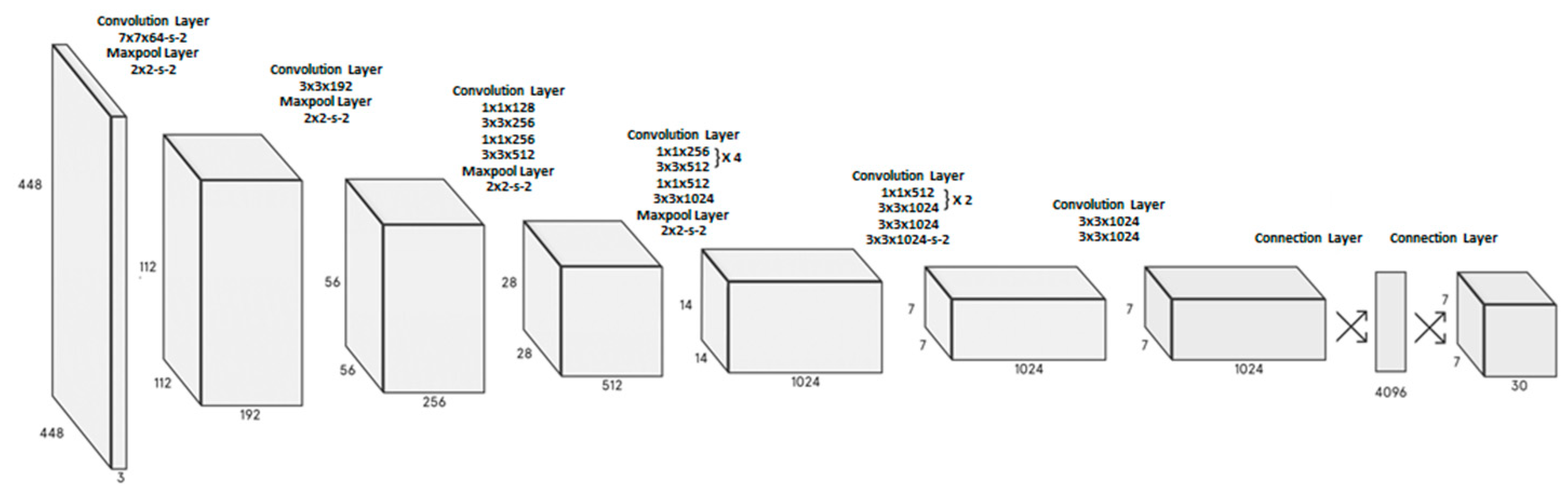
This network consists of 24 convolutional layers and two fully connected layers. To reduce the number of layers, designers employ a 1 × 1 convolution, which makes it possible to decrease the depth of feature maps [31]. A 3 × 3 convolution layer is then applied. These 1 × 1 and 3 × 3 layers alternate. Finally, it is reduced by two fully connected layers, producing an output with a tensioner of size 7 × 7 × 30 (see Figure 1).

The YOLO architecture has evolved from the YOLOv1 version to YOLOv11, released in September 2024, optimizing its performance and accuracy; in the YOLOv5 version, presented in 2020, developed by Ultralytics, not by the original authors, the implementation was conducted on PyTorch [32]. This version maintained YOLO′s original focus, dividing the image into a grid and predicting bounding boxes along with the associated class probabilities for each cell.

In 2022, versions YOLOv6 [33] and YOLOv7 [32] were presented, improving their architecture and training scheme, as well as improving the accuracy of object detection without increasing the cost of inference, using a concept known as “trainable feature bags” [32]. In 2023, YOLOv8 was presented; its improvements include new features, better performance, flexibility, and efficiency, and additionally include improvements for detection, segmentation, pose estimation, tracking, and classification, although there is no official publication in [34] that presents a description of the architecture.

In 2024, the authors of [35] presented YOLOv9, marking a significant advance in real-time object detection, introducing revolutionary techniques such as Programmable Gradient Information (PGI) and the Generalized Efficient Layer Aggregation Network (GELAN). YOLOv9 is developed by an independent open source team based primarily on YOLOv5 [35]. In 2024, Tsinghua University introduced YOLOv10, a version that improves real-time object detection by eliminating Non-Maximum Suppression (NMS) and optimizing model architecture. At the end of 2024, YOLO11, the latest version of the Ultralytics series, was presented, which was designed to offer an exceptional balance between accuracy, speed, and efficiency in object detection. Thanks to advances in its architecture and training methods, YOLO11 improves feature extraction, increases accuracy by reducing the number of parameters, and optimizes both speed and computational efficiency.

Although the YOLO series stands out for its balance between speed and accuracy in real-time object detection, the use of NMS negatively impacts its performance; so, in 2020, the Facebook AI Research (FAIR) team developed the transformer-based DEtection TRansformer (DETR) [36] for object detection and managed to eliminate the NMS, which simplifies the model’s workflow since it does not require a post-processing step to filter redundant predictions.

In 2023, the authors of [37] proposed a RT-DETR (Real-Time Detection Transformer) a real time object detector based on transformer architecture, which was designed to outperform YOLO models through an end-to-end architecture that eliminates the need for NMS. Its core consists of an efficient hybrid encoder and an advanced query selection strategy. The hybrid encoder decouples Attention-based Intra-scale Feature Interaction (AIFI) from convolution-based Cross-scale Feature Fusion (CCFF), which reduces computational redundancy and improves efficiency. In addition, RT-DETR introduces query selection with minimal uncertainty, which optimizes the choice of initial features for the decoder, minimizing the discrepancy between classification and localization predictions. This architecture also allows adjusting the inference speed by modifying the number of decoder layers without retraining, thus adapting to different scenarios in real time.

The RT-DETR model differs from YOLO primarily in its architectural approach and inference processing. While YOLO uses a CNN-based architecture and relies on NMS to filter redundant boxes, which introduces latency and complexity in calibration, RT-DETR is completely end-to-end, eliminating NMS by directly predicting unique sets of objects through bipartite matching. In addition, RT-DETR improves computational efficiency through a hybrid encoder that decouples intra-scale interaction and cross-scale fusion, while YOLO uses structures such as Feature Pyramid Networks for multiscale detection. In terms of performance, RT-DETR outperforms YOLO in both accuracy and speed. According to the results presented in [37], the model demonstrates higher efficiency when pre-trained with the Objects365 large-scale dataset, allowing it to achieve better performance with fewer parameters. In addition, RT-DETR offers greater flexibility to adapt to various scenarios, as it allows adjusting the decoder depth without retraining.

Several studies have analyzed and compared different models of CNNs for the detection of weeds in maize crops; for example, the authors of [38] designed a CNN based on the YOLOv4-tiny model called YOLOv4-weeds, with the objective of detecting weeds in the maize crop; to verify its effectiveness, the results of the mAP were compared with the results of the CNNs Faster R-CNN, SSD 300, YOLOv3, YOLOv3-tiny, and YOLOv4-tiny. The proposed model YOLOv4-weeds obtained the best mAP value of 0.867, while a value of 0.685 was obtained for the Faster R-CNN model, 0.692 for SSD300, 0.855 for YOLOv3, 0.757 for YOLOv3-tiny, and 0.803 for YOLOv4-tiny.

In the study in [39], the authors proposed a lightweight model based on YOLOv5s to build a precision spraying robot for maize cultivation. They used versions YOLOv5s, YOLOv5m, YOLOv5l, and YOLOv5x, comparing their mAP. The best version was YOLOv5s, with a mAP of 0.932 for the maize class and a mAP of 0.859 for weeds. Subsequently, they modified the structure of YOLOv5s by adding a C3-Ghost-bottleneck module, with which they improved the architecture, obtaining a mAP for maize of 0.963 and a mAP for weeds of 0.889.

Likewise, the authors of [40] evaluated the behavior of YOLOv5s in the detection of weeds in maize, obtaining excellent results; in the maize class, a mAP of 0.836 was achieved, which shows that YOLO models are adequate to detect weeds in maize crops. Additionally, work has been conducted with different types of images; for example, the authors of [41] evaluated different versions of the YOLO family, specifically YOLOv4, YOLOv4-tiny, YOLOv4-tiny-3l, and YOLOv5 in versions s, m, and l, with the objective of detecting and counting maize plants in the field with the presence of weeds through images taken with UAVs. The results obtained in mAP show that the best score was for YOLOv5s with a value of 0.731; the other models obtained values of 0.720 for YOLOv4, 0.649 for YOLOv4-tiny, 0.581 for YOLOv4-tiny-3l, 0.716 for YOLOv5m, and 0.685 for YOLOv5l.

Regarding the use of transformer based architecture in weed detection, several investigations have been carried out. The authors of [42] developed the dual-path Swin Transformer model with multi-modal images (RGB and depth) in the wheat crop; this model obtained an increase in pressure of 11% compared to traditional CNNs. Similarly, the authors of [43] presented the CSWin-MBConv model, a hybrid model that combines CNNs and Transformer architectures for accurate identification of different types of weeds in agricultural fields; experiments performed on a weed image dataset showed that CSWin-MBConv outperforms conventional CNN and Transformer models in accuracy, obtaining a 0.985 accuracy and an F1-score of 0.985, outperforming state-of-the-art models such as ResNet-101, DenseNet-161, EfficientNet-B6, and Swin Transformer. As for maize crops, the authors of [44] used transformer based DL architecture for weed detection in maize crops; they compared three semantic segmentation models, Swin-UNet, Segmenter, and SegFormer, to identify and classify weeds at the pixel level. This study concluded that the SegFormer model obtained the best results with an accuracy of 0.949.

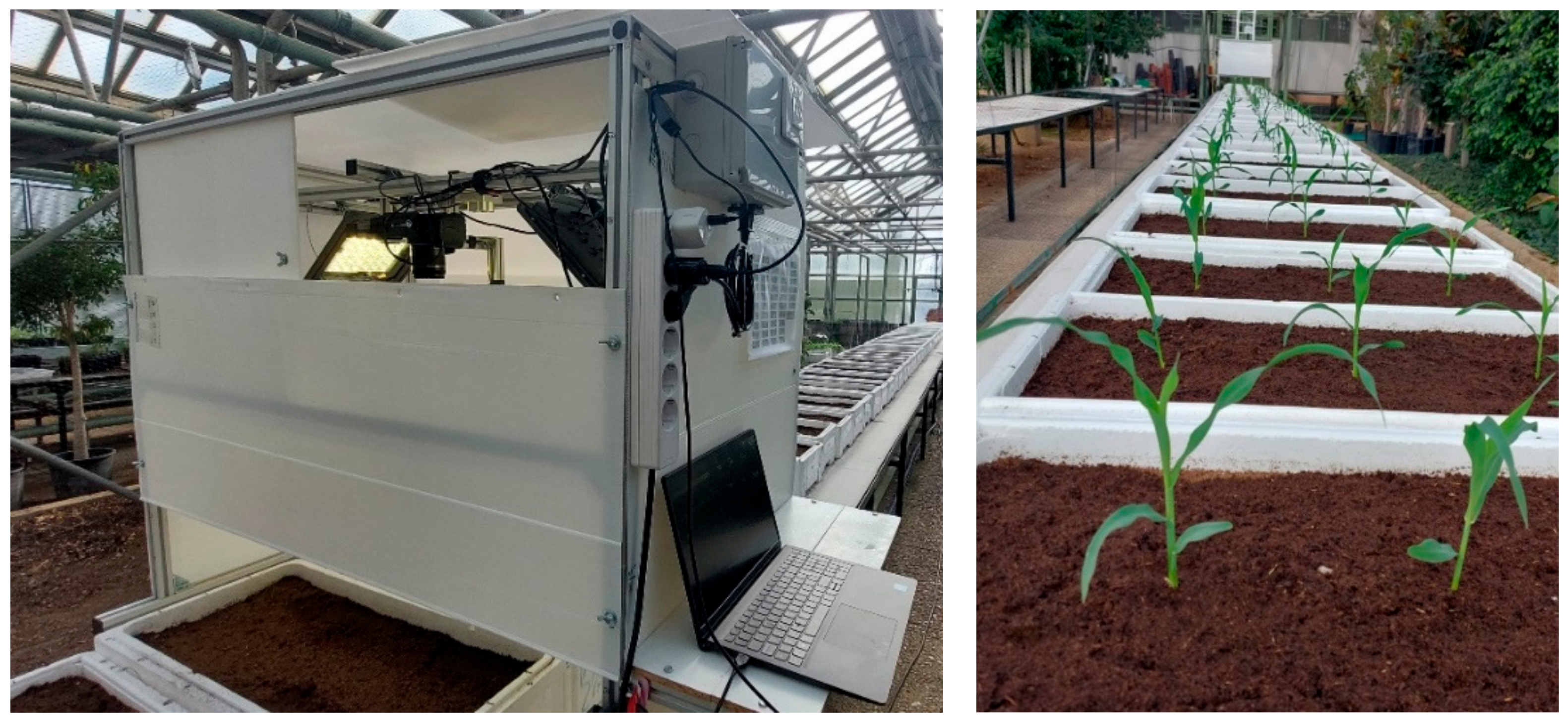
In this work, a performance analysis of the models YOLOv8s, YOLOv9s, YOLOv10s, YOLOv11s, and an RT-DETR-l model is performed; for this, we worked with captured images of maize plants (Zea mays L.) and four species of weeds (Lolium rigidum, Sonchus oleraceus, Saolanun nigrum, and Poa annua) grown in a greenhouse under controlled conditions. In Section 1, the state of the art of the CNN models used is presented; in Section 2, the methodology for the acquisition of the image dataset of the species used is presented, and the configuration of the models training parameters and their measurement metrics is established. In Section 3, the results and analysis are presented, establishing which of the models has the best performance; the evaluation of the performance of the models was carried out through metrics such as precision, recall, F1-score, mAP, and analysis of Precision–Recall curves and confusion matrices, allowing to identify strengths and weaknesses of the models in the different classes evaluated. Section 4 presents the conclusions of this study and future work in order to implement the best model in the development of an automatic weed detection system in maize cultivation.

2. Materials and Methods

For the analysis of the performance of the RT-DETR and YOLO models in the detection of weeds in the maize crop, a methodology was designed that responds to the need to evaluate advanced CNN models in a controlled agricultural production environment, ensuring that the data and experimental configurations are representative, accurate, and comparable.

2.1. Biological Material

Sweet corn seed (Zea mays L.) and four types of weeds (Lolium rigidum, Sonchus oleraceus, Saolanun nigrum, and Poa annua, see Figure 2) were used. The weeds were selected considering their relevance in competition with the maize crop in the study area (Community of Castilla y León, Spain). This selection seeks to strategically represent the main groups of weeds according to their morphology and competitive behavior, selecting both broadleaf weeds (dicotyledons), Sonchus oleraceus and Solanum nigrum, and narrowleaf weeds (monocotyledons), Lolium rigidum and Poa annua.

The experiment was carried out from 4 March to 3 May 2024, in the climate-controlled greenhouse of La Yutera campus, University of Valladolid. During the experiment, the crop was maintained with frequent irrigation and under controlled conditions of a temperature of 24 °C and relative humidity of 60%, as shown in Figure 3. A total of 138 maize seeds were sown on a raised bed substrate distributed in 46 containers, placing three seeds in each container. The plants of maize were maintained until the end of the phenological stage of vegetative development V6 (day 60 after planting); the emergence of the maize plant to state V6 is considered the most sensitive stage of the crop due to the nutrient requirement and its competition with weeds [2,45].

For weeds, they were sown in 2 stages: Step 1: this period consisted of day 0 when the seeds are sown to day 30. In this stage, four types of weeds selected were randomly planted with a distribution of 6 plants around each maize plant, obtaining 12 specimens per container for a total of 552. On day 31, the weeds were eradicated due to size, considering that commercially, the weeds do not exceed this size in cultivation. Stage 2: this period consisted of days 32 to 60, as shown in the detailed timeline in Figure 4. After eradication, the four types of weeds were planted again with a distribution of 9 plants per container, in this case, three for each maize plant, obtaining a total of 414 at this stage, for a total of 966 weed plants in the two stages.

2.2. Image Capture

To capture the images, a support trolley located on the raised bed of the greenhouse was used; the trolley advances on a system of guides that allows controlled displacement. The trolley supports the vision system, which is composed of a Canon 850D SLR camera (Ohta-ku, Canon Inc., Tokyo, Japan), with a 22.3 × 14.9 mm CMOS sensor located one meter high from the crop substrate, and an EF-S 15–55 mm f/4-536 IS STM lens (Tanzi, Canon Inc., Taichung, Taiwán) with PL-C 58 mm circular polarizing filter was used. The system’s lighting consists of two 6000 K type LED white light lamps configured in a 6 × 6 LED matrix, with a transmission ROSCO polarizing filter screen at 38% (1.5 f/stop) to avoid glare on plant leaves, as shown in Figure 3.

RGB images with a resolution of 6000 × 4000 pixels were taken for 35 days, distributed from the moment of the emergence of the plant (day 12) to the end of the phenological stage of vegetative development (day 60), obtaining a total of 1640 images.

2.3. Preprocessing

2.3.1. Selection of Images

The images suitable for training were selected, eliminating those with a high blur or images in which the plant was so large that it was outside of the image frame; these were found in the last days of the vegetative stage, V6. In the selection, 240 images were deleted, leaving 1400 images.

2.3.2. LabelImg of Images

The open source tool LabelImg was used for labeling the images, which allows for saving the labels in YOLO format. Five classes were used, and the labels were defined according to the species used by abbreviating their names: “maize”, for maize plants, “mh1” for Lolium rigidum, “mh2” for Sonchus oleraceus, “mh3” for Solanum nigrum, and “mh4” for Poa annua, as shown in Figure 2. A set of 4200 maize delimiter box labels and 10,322 weed labels were obtained. The labeling was carried out by experts with in-depth knowledge of the species.

2.3.3. Selection of Architectures and Preparation of Data

The RT-DETR-l architectures and the YOLOv8s, YOLOv9s, YOLOv10s, and YOLOv11s models were selected. YOLO architectures are characterized by being used in various agricultural applications, specifically in the cultivation of maize found in the studies reported in [40,46,47]. Within the family of YOLO models, there are different variants (n, s, m, l, and x); the letters refer to the different sizes of pre-trained models available, which vary in the number of parameters and layers, allowing to choose a balance between accuracy, speed, and computational requirements. In this study, we seek to make the analyzed models easily trainable, efficient, and lightweight so that an embedded advanced computing development kit can be implemented. Therefore, we selected the size s “Small”, which is a small model suitable for devices with limited resources (drinking), with a good balance between speed and accuracy, making it suitable for the development of precision weed systems that work in real time. As for the RT-DETR model, the smallest available model was selected, which is the l “Large” version; this model offers greater precision and can handle more types of objects with greater accuracy but requires more computational power. The data were divided equally for all the analyzed models, with 64% for training (896 images), 20% for testing (280 images), and 16% for validation (224 images).

2.3.4. Setting the Parameters for Training

A maximum of 300 training epochs were set for all architectures, using the Early Stopping technique to avoid overfitting. This maximum value was selected from previous experiments, where it was observed that stability in the results was reached around 150 epochs. To ensure that the model had sufficient scope to learn without the risk of overtraining, this 300-epoch upper limit was defined. Early Stopping is a technique that stops training automatically when there are no improvements in the loss of the validation set for a consecutive number of times. This allows for the avoidance of overfitting and saves processing time. This behavior is controlled by the patience parameter, configured in 20 epochs, which is a value that provides enough flexibility for the model to stabilize without unnecessarily extending the training. It should be noted that in the study reported in [48], YOLO architecture was trained with up to 600 epochs, achieving the highest precision. However, using such high values can increase the risk of over-adjustment and significantly prolong the processing time, reinforcing the decision to apply Early Stopping in this case.

The lot size (batch_size) was set to 32, a value that allows the reduction in the overfitting of the model in the initial stages, in addition to increasing the training speed. The size of the images was set at 640 × 640 pixels; although the images used in this study are larger, the YOLO models uniformly reduce the input images to 640 × 640 pixels. The initial learning rate (lr0) and final learning rate (lrf) were set at 0.01, with the weight decay parameter set at 0.0005 and the Momentum set at 0.937. The IoU parameter (Intersection over Union) was set to 0.7. The other hyperparameters used are those defined by the default model recommended in [49].

Table 1. Summary of configuration hyperparameters for training.

epochs	300	iou	0.7	kobj	1.0
patience	20	max_det	300	nbs	64
batch	32	half	false	hsv_h	0.015
imgsz	640	dnn	false	hsv_s	0.7
workers	8	plots	<n	hsv_v	0.4
pretrained	<n	vid_stride	1	degrees	0.0
optimizer	auto	lr0	0.01	translate	0.1
verbose	true	lrf	0.01	scale	0.5
seed	0	momentum	0.937	shear	0.0
deterministic	true	weight_decay	0.0005	perspective	0.0
close_mosaic	10	warmup_epochs	3.0	flipud	0.0
fraction	1.0	warmup_momentum	0.8	fliplr	0.5
mask_ratio	4	warmup_bias_lr	0.1	bgr	0.0
dropout	0.0	box	7.5	mosaic	1.0
val	true	cls	0.5	mixup	0.0
split	val	dfl	1.5	erasing	0.4
conf	null	pose	12.0	crop_fraction	1.0

presents a summary of the hyperparameters used in training for all the models analyzed.

2.3.5. Configuration of the Equipment

For the training, the configuration described in

Table 2. Configuration used for model training.

System Element	Description
Processor	AMD EPYC 7H12 (2595 GHz) (Santa Clara, AMD Inc., California, USA)
GPU	NVIDIA Tesla V100 (Santa Clara, NVIDIA Corp., California, USA)
RAM	64 GB
Accelerated environment	CUDA 12.4
Development environment	Python 3.10.15 PyTorch 2.5.1—Torchvision 0.20.1

was used.

2.4. Evaluation Metrics

2.4.1. Confusion Matrix

The confusion matrix is a fundamental tool for evaluating the performance of classification models, allowing us to analyze how the predictions made by a model are compared with the actual labels of the data. Its basic structure organizes predictions into four main categories:

• True positive (TP): cases in which the model correctly predicts an instance as positive.
• False positive (FP): cases in which the model classifies an instance as positive but is negative.
• False negative (FN): cases in which the model incorrectly classifies a positive instance as negative.
• True negative (TN): cases in which the model correctly predicts an instance as negative.

2.4.2. Metrics Derived from the Confusion Matrix

Based on the values of the matrix, it is possible to calculate key metrics to evaluate the performance of the model as follows:

• Precision represents the ratio of correct positive predictions to all positive predictions made, as shown in Equation (1).

  $$Precision={\displaystyle \frac{TP}{TP+FP}}$$

  (1)
• Recall measures the model’s ability to detect positive instances correctly, as shown in Equation (2).

  $$Recall={\displaystyle \frac{TP}{TP+FN}}$$

  (2)
• Accuracy indicates the ratio of correct predictions, both positive and negative, to total instances, as shown in Equation (3).

  $$Accuracy={\displaystyle \frac{TP+TN}{TP+FP+TN+FN}}$$

  (3)
• The F1-score is the harmonic mean between accuracy and recall, which is especially useful when classes are unbalanced, as shown in Equation (4).

  $$F1\_score=2\left({\displaystyle \frac{Precision\times Recall}{Precision+Recall}}\right)$$

  (4)

2.4.3. Precision–Recall Curve (PR)

The PR curve is a tool for evaluating the performance of object classification and detection models, which can especially detect problems with unbalanced classes. These curves illustrate the relationship between accuracy, which measures the proportion of correct positive predictions, and recall, which indicates the proportion of real objects detected correctly. As the model’s confidence threshold is adjusted, accuracy and recall change, allowing the PR curve to be constructed. An optimal model maintains high accuracy and recall at all thresholds, generating a curve close to the upper right vertex. The usefulness of PR curves lies in their ability to compare models, identify optimal thresholds, and evaluate performance in scenarios with unbalanced data. In addition, derived metrics such as the Average Precision (AP), which calculates the area under the PR curve, and the mAP, which averages the AP for all classes, provide a quantitative assessment of the model.

2.4.4. F1-Score Curve—Confidence

The F1-score—Confidence curve allows a graphical assessment of how the F1-score of a model varies based on the confidence threshold used to classify its predictions. The F1-score, calculated as the harmonic mean between accuracy and recall, is a key metric in problems where both metrics are equally important, especially in contexts with unbalanced classes. By comparing the F1-score with the confidence threshold, a clear representation of the trade-off between accuracy and recall at different confidence levels is obtained, which facilitates the selection of the optimal threshold that maximizes model performance. This curve has practical applications in object detection, classification, and critical decision systems, where finding the right threshold is essential to avoid false positives or negatives depending on the context. In addition, it allows us to compare the robustness of different models to identify weak points and optimize the overall performance. The maximum point of the curve indicates the optimal confidence threshold, while the slope reflects the sensitivity of the model to changes in the threshold, providing a comprehensive assessment of its behavior.

2.4.5. Metrics Average Precision (AP) and Mean Average Precision (mAP)

The AP is a standard metric used in the evaluation of object detection models, which measures the trade-off between accuracy and recall as a function of different confidence thresholds. It is calculated as the area under the Precision–Recall curve for a specific class, providing a comprehensive measure of the model’s performance in correctly classifying and locating objects, as shown in Equation (5). An AP close to 1 indicates excellent performance, while low values reflect model difficulties in balancing accuracy and recall.

$$\mathrm{A}\mathrm{P}={\sum }_{\mathrm{n}=1}^N\left({\mathit{R}}_{\mathit{n}}-{\mathit{R}}_{\mathit{n}-1}\right) \mathrm{\ast } {\mathit{P}}_{\mathit{n}}$$

(5)

where:

N: Number of discrete points on the Precision–Recall curve.

R_n: Recall value at point n.

R_n−1: Recall value at the previous point (n − 1).

P_n: Precision value corresponding to point n.

The mAP is an integral metric because it considers the quality of predictions (precision) and the model’s ability to detect objects in the validation set (recall). Combining these aspects into a single value allows us to objectively compare different models or configurations, which makes it the reference standard for detection tasks; it is calculated as the average of the AP values obtained for all classes, as shown in Equation (6).

$$\mathrm{m}\mathrm{A}\mathrm{P}={\displaystyle \frac{1}{N}}{\sum }_{n=1}^{N}APn \mathrm{w}\mathrm{h}\mathrm{e}\mathrm{r}\mathrm{e} APn={\int }_0^{1}P\left(R\right)dR$$

(6)

where

N: Number of classes.

APn: Average Precision of class n.

2.4.6. Metric Intersection over Union (IoU)

The IoU metric quantifies the overlap between a predicted bounding box and the actual ground truth, providing an objective measure to determine how well the model locates an object, calculated as the ratio between the intersection area and the junction area of the two boxes, Equation (7).

$$IoU={\displaystyle \frac{\mathrm{A}\mathrm{r}\mathrm{e}\mathrm{a} \mathrm{o}\mathrm{f} \mathrm{i}\mathrm{n}\mathrm{t}\mathrm{e}\mathrm{r}\mathrm{s}\mathrm{e}\mathrm{c}\mathrm{t}\mathrm{i}\mathrm{o}\mathrm{n}}{\mathrm{A}\mathrm{r}\mathrm{e}\mathrm{a} \mathrm{o}\mathrm{f} \mathrm{j}\mathrm{u}\mathrm{n}\mathrm{c}\mathrm{t}\mathrm{i}\mathrm{o}\mathrm{n}}}$$

(7)

where

Joining area: This is the total area covered by both boxes, excluding the intersection.

Intersection area: This is the common area between the predicted box and the actual box.

Interpretation of the IoU is essential to understand and improve the performance of a model in object detection tasks. When evaluating the overlap between the predicted boxes and the actual boxes, the IoU value is always between 0 and 1, showing a partial overlap between the prediction and the actual box; if IoU is equal to 1, the prediction exactly matches the actual box, if IoU is equal to 0, there is no intersection between the prediction and the actual box. The IoU is widely used with predefined thresholds to classify predictions into object detection tasks. These thresholds determine whether a prediction made by the model is considered correct or incorrect based on the degree of overlap between the predicted bounding box and the actual box. A threshold of 0.5 is generally used since it provides a practical balance between accuracy and flexibility when evaluating the predictions of the model, and a classification of predictions is established as follows:

• IoU ≥ 0.5: This result is considered a correct prediction TP.
• IoU < 0.5: This result is considered an incorrect prediction FP.
• IoU = 0: If there is no prediction for a real object, it is classified as an FN.

3. Results and Discussion

This section presents and analyzes the results obtained after training the models YOLOv8s, YOLOv9s, YOLOv10s, YOLOv11s, and RT-DETR-l in the detection of maize plants and four types of weeds under controlled conditions. The results include metrics such as precision, recall, F1-score, mAP, confusion matrix, and the Precision–Recall and F1-score—Confidence curves, allowing the identification of the individual performance of each model in the different classes, as well as the strengths and limitations of each model according to its computational efficiency and generalization capacity.

3.1. Results of the Confusion Matrix

As part of the analysis of the performance of the models, the confusion matrix in absolute values was used to evaluate the behavior of the predictions of the model based on the true classes and the predicted classes. Also, the normalized confusion matrix was calculated, which scales the values to proportions or percentages and does not directly depend on the size of each class.

3.1.1. Confusion Matrices for the Model YOLOv8s

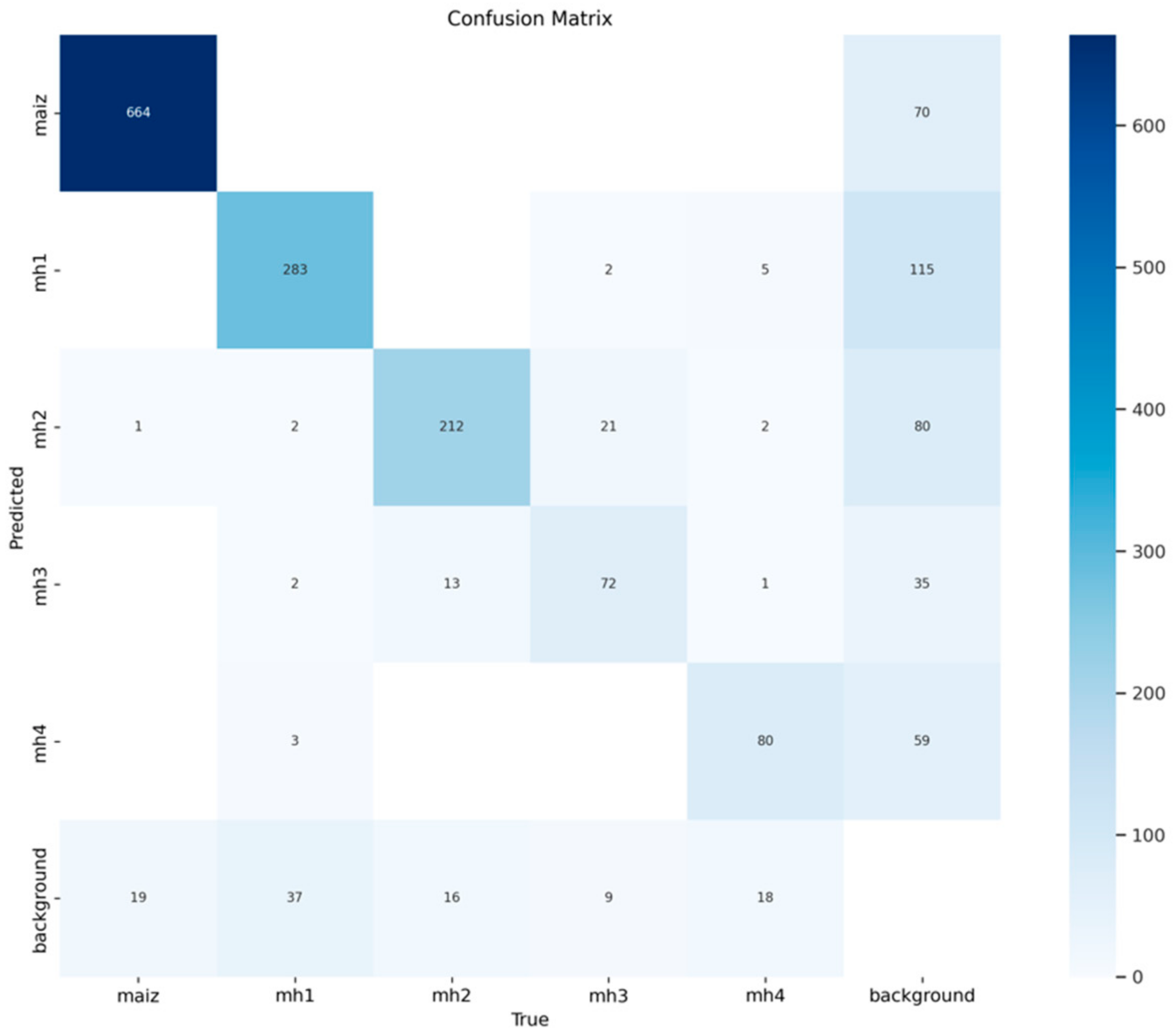
In Figure 5, it can be observed that the YOLOv8s model has a solid performance in the detection of the maize class, with 664 true positives, which represents a high ability to identify this class correctly. However, 70 false positives for “background” indicate that the model is confusing elements present in the background with maize. Likewise, 19 false negatives are presented; in this case, they would be instances of maize that the model does not detect and classifies as background. The accuracy was calculated at 0.905, which indicates that the model presents a moderate rate of false positives, erroneously classifying some elements of the background as maize. As for recall at 0.972, it reflects its ability to identify almost all real instances of this class in images.

Regarding the standard confusion matrix for the YOLOv8s model shown in Figure 6, the “maize” class shows that 0.97 of the maize instances were correctly classified as “maize”. However, it has 0.03 false negatives (i.e., samples from the maize class are not identified as any other class but are considered “background”). This is an excellent result since the YOLOv8s model identified the “maize” class with great precision, with minimal confusion with the background and no significant errors with other classes. However, there are 0.32 false positives with the background.

Regarding the class “mh1”, it has an acceptable performance, with 283 true positives. However, the 115 false positives for “background FP” represent a significant challenge to the accuracy of this class, which reaches only 0.711. This indicates that the visual characteristics of “mh1” are not sufficiently distinctive for the model compared to the background. In addition, the 37 false negatives for “background FN” affect recall, which stands at 0.884, showing that the model loses some real instances of “mh1”. In general, the YOLOv8s model shows that 0.87 of the “mh1” instances were correctly classified; it is a good performance. However, it has 0.11 false negatives and 0.03 with the other classes (see Figure 6).

The detection of the “mh2” class has a relatively good performance, with 212 true positives and 16 false negatives for “background FN”, resulting in a recall of 0.93, indicating that the model correctly identified most of the real instances of this class. However, the 80 false positives at the bottom for “background FP” affect the accuracy, which is reduced to 0.726. This result suggests that the model is confusing the visual characteristics of “mh2” with those of the background. In general, the class “mh2” of the YOLOv8s model showed that 0.88 of the instances of “mh2” were correctly classified and 0.07 were false negatives for “background FN”. Including more examples with variations of the “mh2” class in the dataset could help improve the model’s ability to distinguish this class from the others and the background.

The “mh3” class with 72 true positives is one of the classes with the weakest performance, with 35 false positives for “background FP”, indicating that the model has difficulty differentiating this class of elements from the environment, which leads to an accuracy of 0.673. The nine false negatives for “background FN” also affect performance, although to a lesser extent, reaching a recall of 0.889. In general, the YOLOv8s model classifies 0.69 of the instances of the “mh3” class correctly. It is important to mention that this class “mh3” has a 0.2 of true negatives with the class “mh2”. This result is logical due to the similarity between them; the two are wide leaves that are usually confused in the early stages of growth. The results could be improved by increasing the number of examples of “mh3” in training.

The “mh4” class shows a slightly moderate performance, with 80 true positives and 59 false positives for “background FP”, for an accuracy of 0.576, indicating that the model frequently confuses real background instances with the “mh4” class. This can be attributed to visual similarities or an insufficient representation of this class in the training set. In addition, the 18 false negatives for “background FN” and the recall of 0.819 reflect that the model loses real instances of “mh4”. In general, the YOLOv8s model shows that 0.75 of the “mh4” instances were correctly classified as “mh4”; however, it has 0.17 false negatives and 0.16 false negatives, although this “mh4” class performs better than “mh3”. The “mh4” class has considerable confusion with the background. This result could be improved by increasing the examples of this class in the training set and adjusting the training parameters of the model.

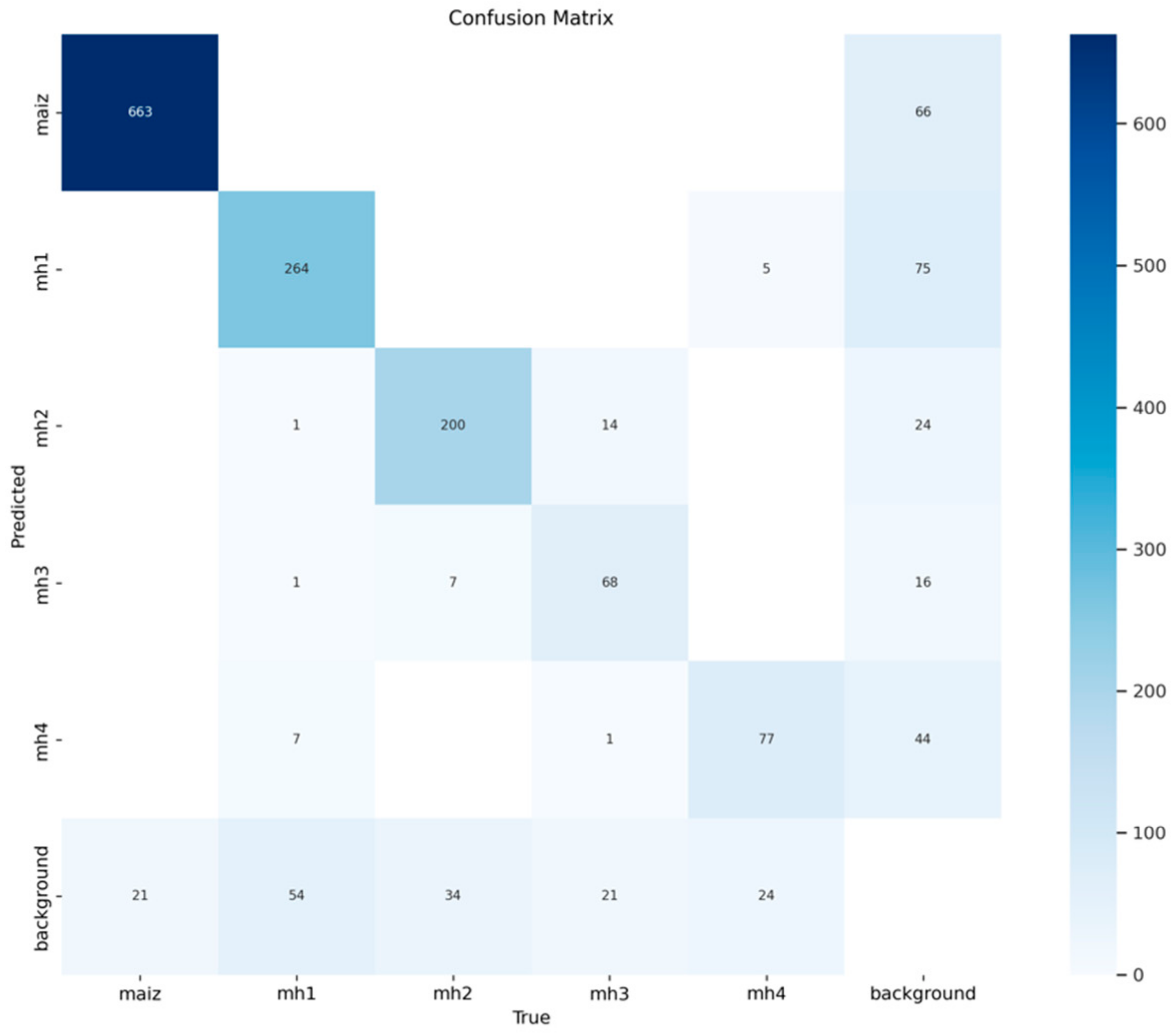
3.1.2. Confusion Matrices for the Model YOLOv9s

Figure 7 shows the confusion matrix with absolute values for the YOLOv9s model, showing a robust performance in detecting the “maize” class, achieving 663 true positives. This indicates that it correctly identified most instances of this class. However, there are 66 false positives for “background FP”, which reflects that the model incorrectly classifies certain instances of the background as maize. On the other hand, there are 21 false negatives for “background FN”, which represent real instances of maize that the model fails to detect, classifying them as background. With these results, the model reaches an accuracy of 0.909 and a recall of 0.969, demonstrating its high ability to identify maize accurately and exhaustively. 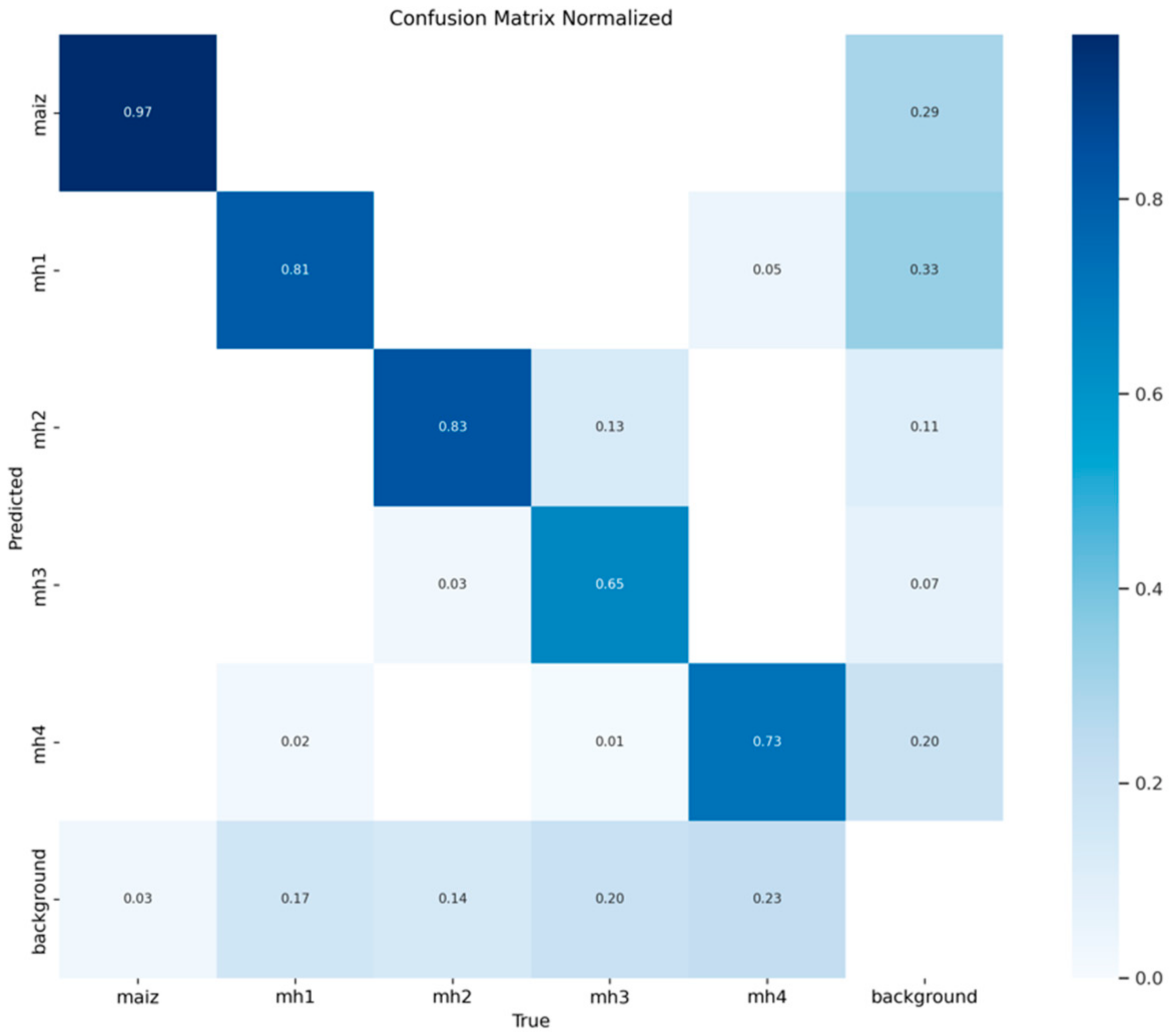Figure 8 shows the standard confusion matrix for the YOLOv9s model, which shows that 0.97 of the instances of the “maize” class were correctly classified as “maize”; on the contrary, the model presented 0.03 false negatives for “background”, as in the YOLOv8s model, which is an excellent result, since it allows the “maize” class to be identified with great precision, without errors with the other classes. However, it presents a 0.29 false positive, which is lower than the YOLOv8s model.

In the detection of the mh1 class, the YOLOv9s model achieves 264 true positives, demonstrating good performance in this class. However, the 75 false positives for “background FP” stand out as a significant source of error, indicating that the model confuses elements of the background with this class. In addition, there are 54 false negatives for “background FN”, representing real instances of “mh1” incorrectly classified as background. These metrics translate into an accuracy of 0.779 and a recall of 0.830, showing a reasonable, although not optimal, balance in recognizing this class. Regarding the standardized data, in Figure 8, the class “mh1” shows a good performance, with 0.807 of the instances correctly classified as “mh1”. However, 0.165 of the real instances of “mh1” were classified as false negatives, which indicates an area of improvement in the detection of this class. There is also a 0.047 degree of confusion with the class “mh4”, which could be due to the similarity of being broad-leaved. False positives reach 0.33 for “background”, indicating that the model needs a greater distinction between this class and the background.

In detecting the “mh2” class, the model achieves 200 true positives, indicating that it correctly identified most instances of this class. However, there are 24 false positives for “background FP”, suggesting that some elements of the background are wrongly classified as “mh2”. On the other hand, there are 34 false negatives for “background FN”, representing real instances of “mh2” incorrectly classified as background. With these results, the model reaches an accuracy of 0.893 and a recall of 0.855, reflecting a good balance between precision and completeness. In general, the class “mh2” has a good performance, with 0.83 of the instances classified correctly, as shown in Figure 8. However, there are 0.141 false negatives and 0.135 false negatives with the class “mh3”. In addition, the 0.107 false positives for “background” indicate that the model also confuses instances of other classes as if they were “mh2”.

The “mh3” class has a more limited performance, with 68 true positives, indicating greater difficulty in correctly identifying this class. In addition, there are 16 false positives for “background FP”, reflecting a significant confusion between background and “mh3”. The 21 false negatives for “background FN” indicate that a considerable proportion of actual instances of “mh3” are not detected, which affects recall. The resulting metrics are an accuracy of 0.810 and a recall of 0.764, showing that this class is less accurate and exhaustive compared to the others. In general, looking at Figure 8, the class “mh3” has the lowest performance, with only 0.654 of the instances classified correctly. The YOLOv9s model confuses 0.20 of the actual instances of “mh3” with “background” and 0.135 with the class “mh2”. This indicates that the classes “mh3” and “mh2” have similar characteristics, which is logical as both species are narrow leaves. As for the false positives related to “background” being less than 0.071, although it is a low value, it is necessary to improve the model in the detection of this class.

In the “mh4” class, the YOLOv9s model achieves 77 true positives, which demonstrates reasonable performance, but presents 44 false positives for “background FP”, suggesting that the model sometimes misclassifies background elements as “mh4”. In addition, there are 24 false negatives for “background FN”, which reflect real instances of “mh4” that the model does not detect. This results in an accuracy of 0.636 and a recall of 0.762, showing that although the model identified a reasonable proportion of the actual instances of “mh4”, its ability to avoid errors is limited. Figure 8 shows that the “mh4” class performs reasonably, with 0.726 instances correctly classified. However, the model confuses 0.226 of the real instances with “background” and 0.1 confusion with the “mh3” class. Although the model correctly detects most instances of “mh4”, the high percentages of false positives (0.196) and negatives show that there is room for improvement in the detection and differentiation of this class.

3.1.3. Confusion Matrices for the Model YOLOv10s

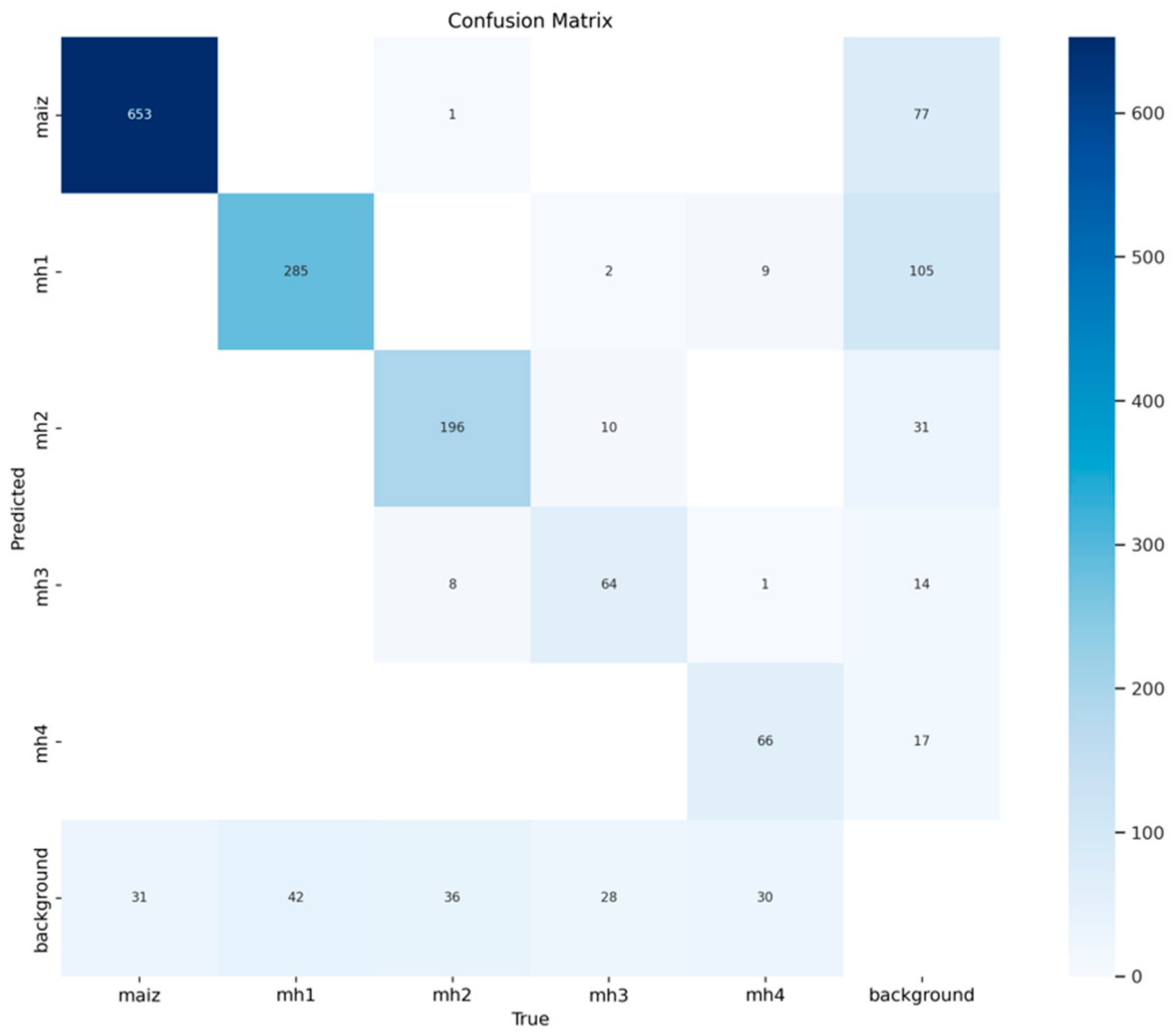
In Figure 9, model YOLOv10s correctly identified 653 true positives of the “maize” class. However, it presented 77 false positives for “background FP”, classifying other classes as “maize”, and 31 false negatives for “background FN”, where real instances of “maize” were classified as background. These results result in an accuracy of 0.895 and a recall of 0.955, showing that the model has a solid and reliable performance for this class. 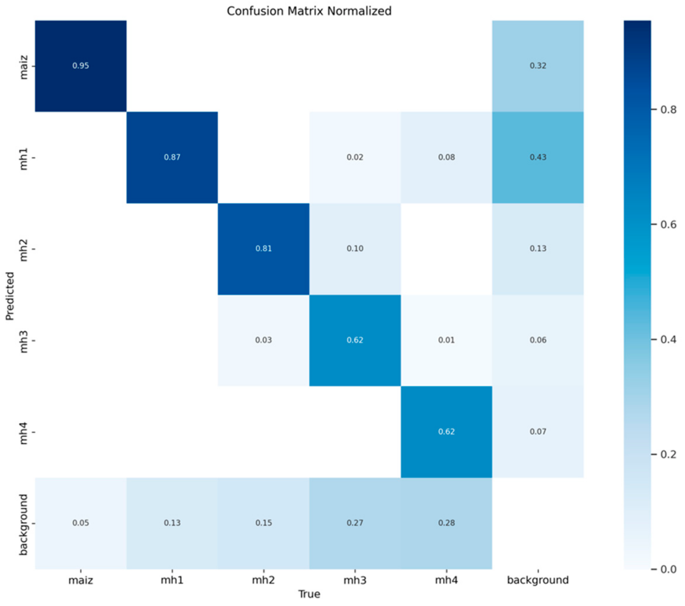Regarding the standard confusion matrix, as shown in Figure 10, 0.955 of the instances of the “maize” class were correctly classified, while 0.045 were confused with other classes, mainly with “background”. This shows that the model is highly effective in detecting this class, with an excellent balance between accuracy and recall.

In the class “mh1”, Figure 9 shows that the YOLOv10s model achieved 285 true positives for the class “mh1”, but with 105 false positives for “background FP” and 42 false negatives for “background FN”, reflecting a more moderate performance. This results in an accuracy of 0.731 and a recall of 0.872, showing that the model faces challenges distinguishing “mh1” from other classes, especially from “background”. In the standard confusion matrix, Figure 10 shows that 0.872 of the instances of “mh1” were correctly classified. However, 0.128 of the instances were confused, mainly with “background” and, to a lesser extent, with “mh4”. This performance indicates that while the model performs well overall, it could benefit from improvements to reduce confusion.

In the “mh2” class, the YOLOv10s model correctly identified 196 true positives, with 31 false positives for “background FP” and 36 false negatives for “background FN”. These results generate an accuracy of 0.863 and a recall of 0.845, highlighting a strong performance for this class with relatively low error rates. Figure 10 shows that 0.813 of the “mh2” instances were correctly classified. The errors of 0.187 in total were mainly distributed between confusions with “mh3” and “background”. This shows that the model has a reasonably high ability to identify this class.

Figure 9 shows 64 true positives for class “mh3”, but 14 false positives for “background FP” and 42 false negatives for “background FN”. This results in an accuracy of 0.821 and a recall of 0.696, reflecting that the model struggles with accuracy, although it is reasonably exhaustive in detecting this class. Regarding the standardized confusion matrix, Figure 10 shows that 0.615 of the “mh3” instances were correctly classified, while 0.385 of the instances were mainly confused with “mh2” and “background”.

Regarding the class “mh4”, it can be seen from Figure 9 that the YOLOv10s model achieved 66 true positives, but also showed 17 false positives for “background FP” and 30 false negatives for “background FN”. This results in an accuracy of 0.795 and a recall of 0.688, indicating that the model has acceptable performance, although it faces challenges in identifying this class accurately. Its performance in terms of the standardized confusion matrix, as shown in Figure 10, indicates that 0.623 of the “mh4” instances were correctly classified, but 0.377 were mainly confused with “background”.

3.1.4. Confusion Matrices for Model YOLOv11s

Figure 11 shows that the YOLOv11s model achieved an accurate detection of the “maize” class, reaching 667 true positives and 73 false positives for “background FP”. However, the model also showed 17 false negatives for “background FP”, indicating that certain instances of “maize” were classified as “background”. These results allow an accuracy of 0.901 and a recall of 0.975 to be calculated, reflecting the model’s high ability to correctly identify “maize” while maintaining a low false negative rate. In Figure 12, 0.975 of the “maize” instances were correctly classified, which underlines the robustness of the model to identify this class without being confused with other categories or the background, and only 0.025 of the “maize” instances were erroneously classified as “background”.

In Figure 11, the YOLOv11s model correctly identified 285 instances of “mh1” but also produced 140 false positives for “background FP” and 40 false negatives for “background FN”. This performance translates into an accuracy of 0.670 and a recall of 0.877, indicating that, although the model correctly detects many instances of “mh1”, there is significant confusion with “background” and other classes. With regard to the standard confusion matrix, as shown in Figure 12, 0.872 of the mh1 instances were correctly classified, and 0.128 errors were due to the erroneous classification as “background” or “maize”. This highlights the need to improve the separation between mh1 and the background, especially when background data have similar visual characteristics.

Regarding the class “mh2”, Figure 11 shows that the YOLOv11s model achieved an identification of 212 true positives and 43 false positives for “background FP”, and 22 false negatives for “background FN” were also recorded. This generates an accuracy of 0.831 and a recall of 0.906, which indicates a good overall performance, although some errors persist, especially with the background. In the normalization of the matrix (Figure 12), 0.88 of the instances of “mh2” were correctly classified, highlighting a superior performance in terms of the identification of this class. A total of 0.12 errors were presented, which were distributed between “background” and “mh3”.

In the “mh3” class, model YOLOv11s correctly identified 65 true positives for “mh3”, but committed 26 false positives to “background FP” and 18 false negatives to “background FN”. This results in an accuracy of 0.714 and a recall of 0.783. In the standard matrix, as shown in Figure 12, 0.625 of the “mh3” instances were correctly classified but 0.375 of the errors were mainly distributed between confusions with “mh2” and “background”, reflecting the difficulties that the model faces in separating this class from the background and other classes.

Figure 11 shows that model YOLOv11s achieved an adequate detection of 77 instances of “mh4”, with 59 false positives for “background FP” and 17 false negatives for “background FN”. This performance leads to an accuracy of 0.566 and recall of 0.794, indicating that the “mh4” class presents a considerable challenge in terms of detection. The model has shown a tendency to confuse “mh4” with “background” and “mh3”. In Figure 12, the standardized confusion matrix shows 0.726 instances of “mh4” correctly classified, but 0.274 of the errors were caused by confusion with “background” and “mh3”.

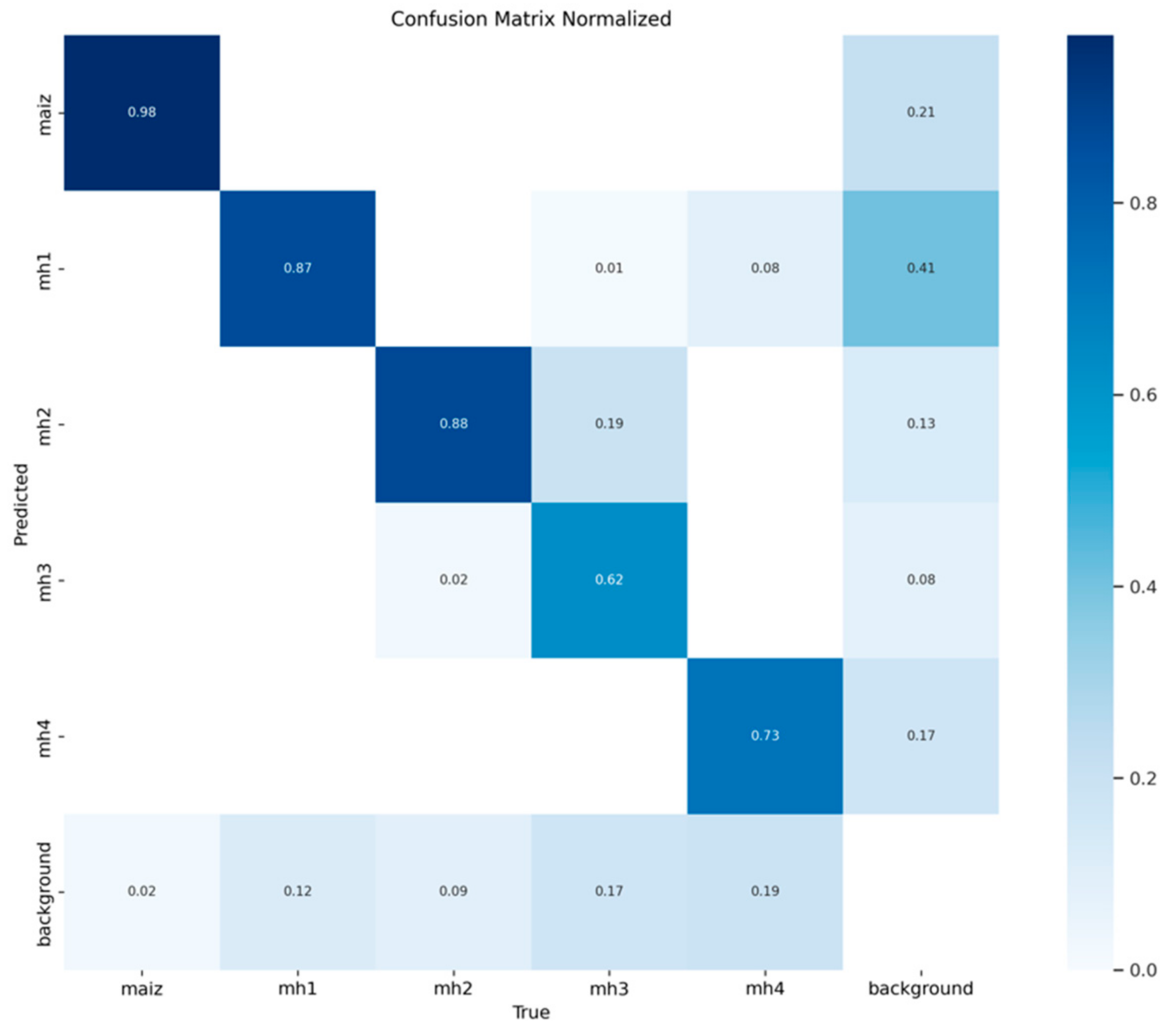
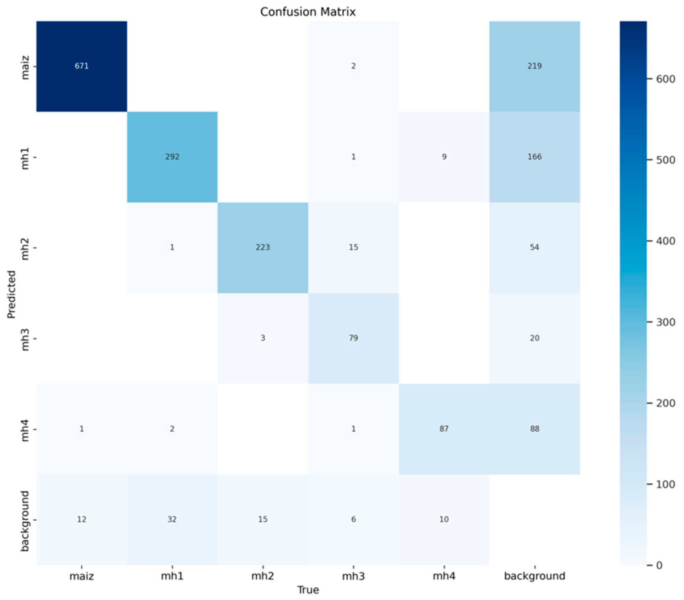
3.1.5. Confusion Matrices for the RT-DETR-l Model

Figure 13 shows that the RT-DETR-l model correctly identified 671 true positives of the “maize” class, while there were 219 false positives for “background FP” and 12 false negatives for “background FN”. These results provide an accuracy of 0.754 and a recall of 0.982. The RT-DETR-l model shows a higher number of false positives than the YOLO models in this class, although the recall is high, showing a high ability to identify instances of “maize” by sacrificing false positives. Regarding the standardized confusion matrix, Figure 14 shows that the 0.981 of the “maize” instances were correctly classified, while 0.019 were confused with other classes, mainly with “background”. This highlights robust performance in terms of recall, although the high rate of false positives negatively affects accuracy.

In class “mh1”, the RT-DETR model detected 292 true positives, 166 false positives for “background FP”, and 32 false negatives for “background FN”, resulting in an accuracy of 0.637 and a recall of 0.901. As in the previous class, although the model identified most instances of “mh1”, it showed a considerable number of false positives. With the normal values, as shown in Figure 14, 0.893 of the instances of “mh1” were correctly classified, while 0.107 were confused, mostly with “background” and, to a lesser extent, with “maize” or “mh4”.

In Figure 13, the RT-DETR model identified 223 true positives for “mh2”, with 54 false positives for “background FP” and 15 false negatives for “background FN”, resulting in an accuracy of 0.805 and a recall of 0.937. This performance reflects a strong ability to classify this class correctly. The standard values, as shown in Figure 14, show that 0.925 of the instances of “mh2” were correctly classified, and 0.075 of errors were distributed between “mh3” and “background”.

In class “mh3”, the RT-DETR-l model correctly identified 79 true positives, 20 false positives for “background FP” and 6 false negatives for “background FN”, obtaining an accuracy of 0.798 and a recall of 0.929. Although these results are good, the false positives with “background” and “mh2” indicate some confusion in the separation between these classes. In Figure 14, the normalized values show that 0.760 of the “mh3” instances were correctly classified, with 0.24 errors, mainly with “background”. In Figure 13, the RT-DETR-l model identified 87 true positives for “mh4”, but presented 88 false positives for “background FP” and 10 false negatives for “background FN”, resulting in an accuracy of 0.497 and a recall of 0.897. This reflects that, although the model is exhaustive in identifying “mh4”, its accuracy is affected by a high rate of false positives. The standard values show that 0.821 of the instances of “mh4” were correctly classified, while 0.179 of the errors were distributed between “background” and other classes as “mh1”.

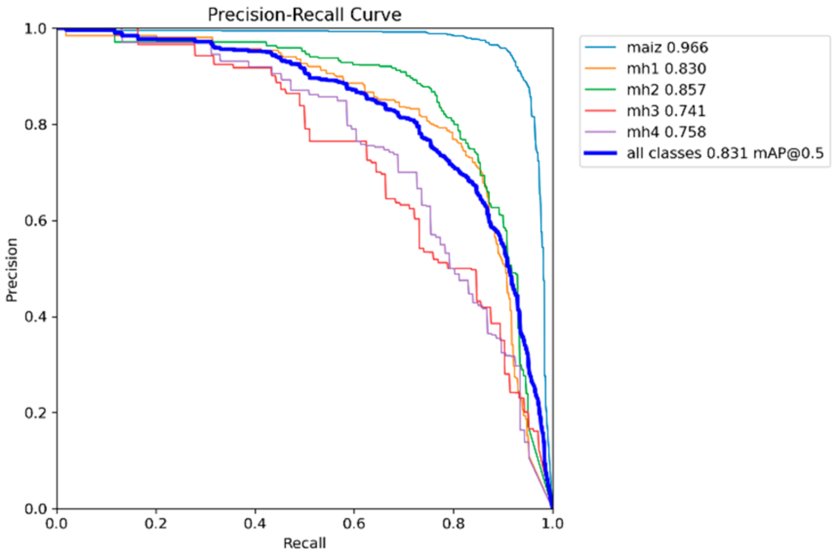
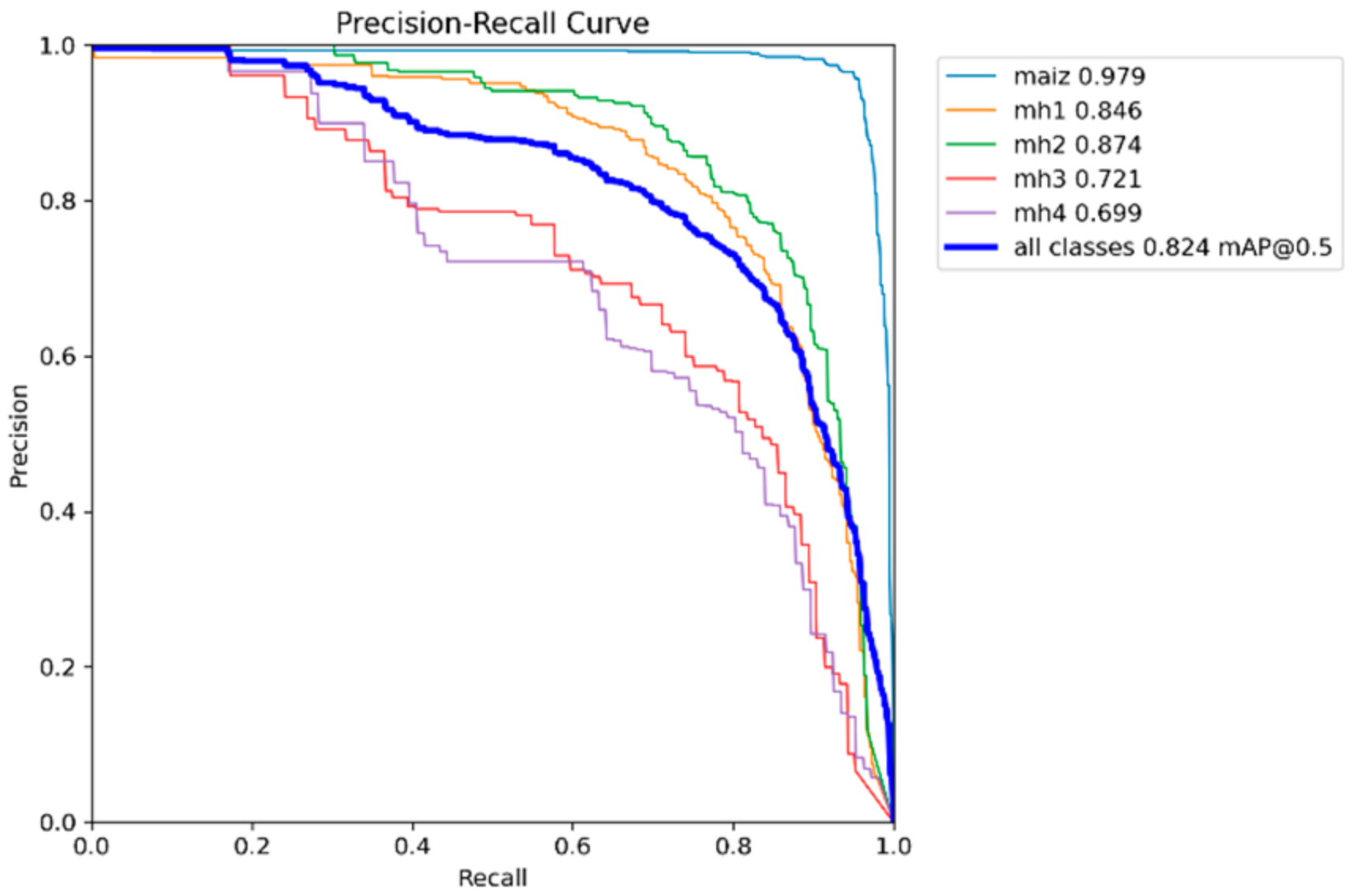
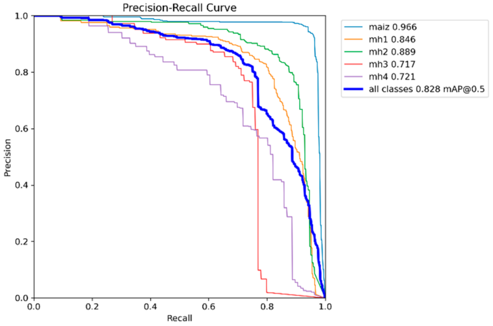
3.2. Precision–Recall Curves

The Precision–Recall curve makes it possible to evaluate the performance of classification models, especially when unbalanced classes are presented; each point on the curve corresponds to a combination of precision and recall for a specific threshold.

As this threshold changes, the accuracy and recall rates also change, and the curve plots show how this relationship behaves. A high curve to the right indicates a good balance between accuracy and recall. In Figure 15, Figure 16, Figure 17, Figure 18 and Figure 19, the precision and recall relationship is presented for each model used, calculating the mAP at an IoU of 0.5 for each class, which is considered a correct prediction if the overlap is at least 50%. Additionally, the mean of mAP@0.5 is calculated for all classes to obtain the general mAP of the model.

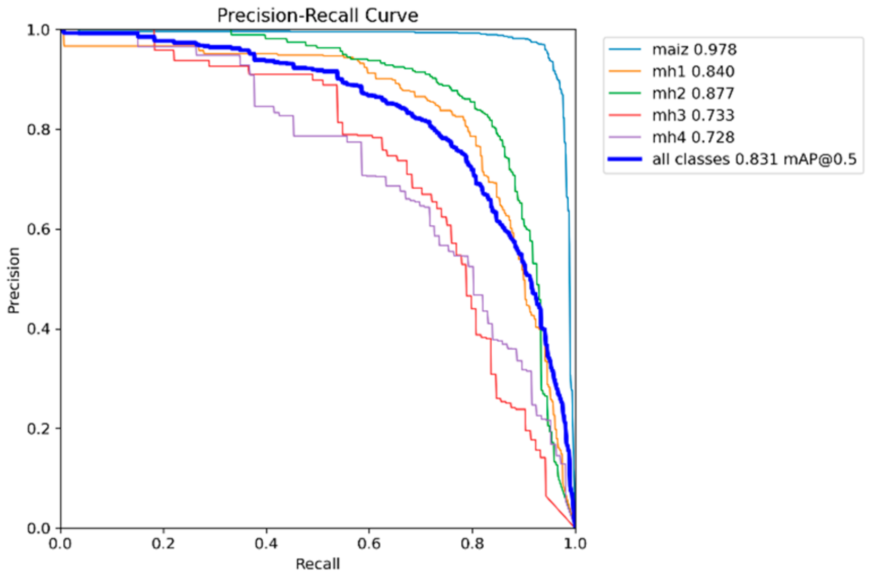
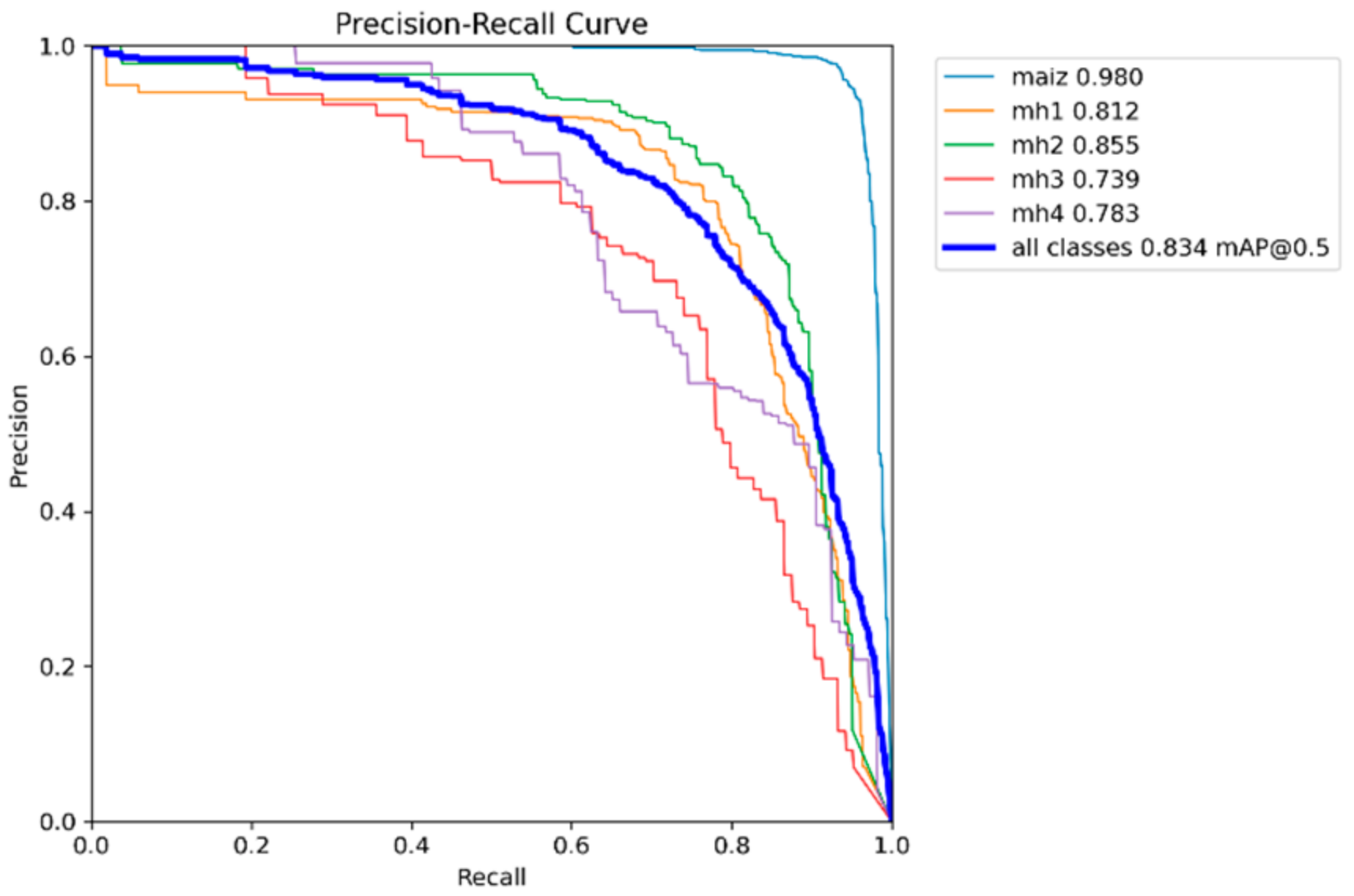
It can be seen that the “maize” class in all the models is the one with the highest curve and to the right, while the classes “mh3” and “mh4” did not perform well.

Table 3. Values of mAP@0.5 for each class of the analyzed models, the data highlighted in bold show the largest mAP@0.5 for each class.

CLASS	YOLOv8s	YOLOv9s	YOLOv10s	YOLOv11s	RT-DETR-l
maize	0.978	0.980	0.966	0.979	0.966
mh1	0.840	0.812	0.830	0.846	0.846
mh2	0.877	0.855	0.857	0.874	0.889
mh3	0.733	0.739	0.741	0.721	0.717
mh4	0.728	0.783	0.758	0.699	0.721
All classes	0.831	0.834	0.831	0.824	0.828

shows the values of mAP@0.5 calculated from the Precision–Recall graphs for the five models YOLOv8s, YOLOv9s, YOLOv10s, YOLOv11s, and RT-DETR-l. These values indicate the average performance of each model for each class and for all classes combined; the higher the value of mAP@0.5, the better the performance of the model.

For the “maize” class, the highest performance was obtained with the YOLOv9s model with 0.98 of mAP@0.5; all models achieve excellent performance in this class, with mAP@0.5 higher than 0.96, reflecting that it is a class for which all trained models show great performance. Regarding the class “mh1”, there is a tie between the models with higher performance, YOLOv11s and RT-DETR-l, both with values of 0.846. Compared to the other models, there is a slight variation in performance; although the performance is acceptable, the performance of YOLOv9s falls, possibly due to confusion with other classes. The “mh2” class obtained the best performance with the RT-DETR-l model with 0.889, followed by the YOLOv8s model with 0.840. In the “mh3” class, the model with the highest performance was YOLOv10s with 0.741, followed by YOLOv9s with 0.739, with values very similar between them; this class presents the greatest challenge for all models since all have mAP@0.5 below 0.75. Confusion with the background or with other classes is probably the cause. In the “mh4” class, the highest performance model was YOLOv9s with 0.783; the performance in this class is variable, with YOLOv9s standing out significantly, while YOLOv11s has a lower performance. As for the overall performance of the model, the highest performance was YOLOv9s with 0.834; all models have similar overall performance, with minor differences in the average, with mAP@0.5 higher than 0.82. The RT-DETR-l model also stands out with 0.828, showing superiority in the classes “mh1” and “mh2”.

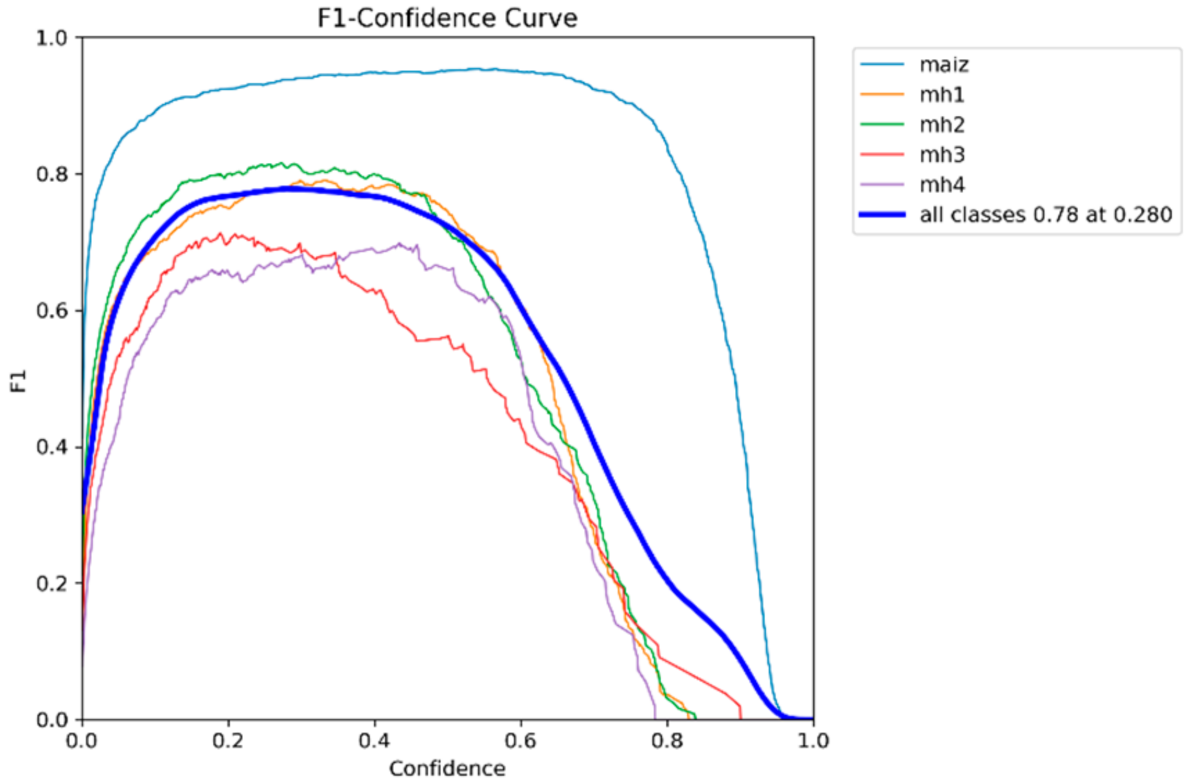
3.3. F1-Score–Confidence Curves

The F1-score–Confidence curve allows the performance of classification models to be assessed against the confidence thresholds applied to their predictions. This graph shows how F1-score, a metric that balances accuracy and recall, varies across different confidence levels for each class in a multiclass dataset. By analyzing these curves, optimal confidence thresholds can be identified that maximize model performance, providing detailed insight into the model’s ability to handle uncertainty in its predictions and enabling fine adjustments to improve the accuracy and recall of each class individually.

Figure 20, Figure 21, Figure 22, Figure 23 and Figure 24 show the values of the confidence thresholds of each model used and their balance between accuracy and recall, plus each curve shows the overall F1-score (for all classes combined) to an optimal confidence threshold of balancing between accuracy and recall.

Table 4. F1-score values for the balanced confidence thresholds of the analyzed models.

MODEL	F1-Score	Confidence Threshold
YOLOv8s	0.78	0.400
YOLOv9s	0.78	0.280
YOLOv10s	0.77	0.269
YOLOv11s	0.76	0.316
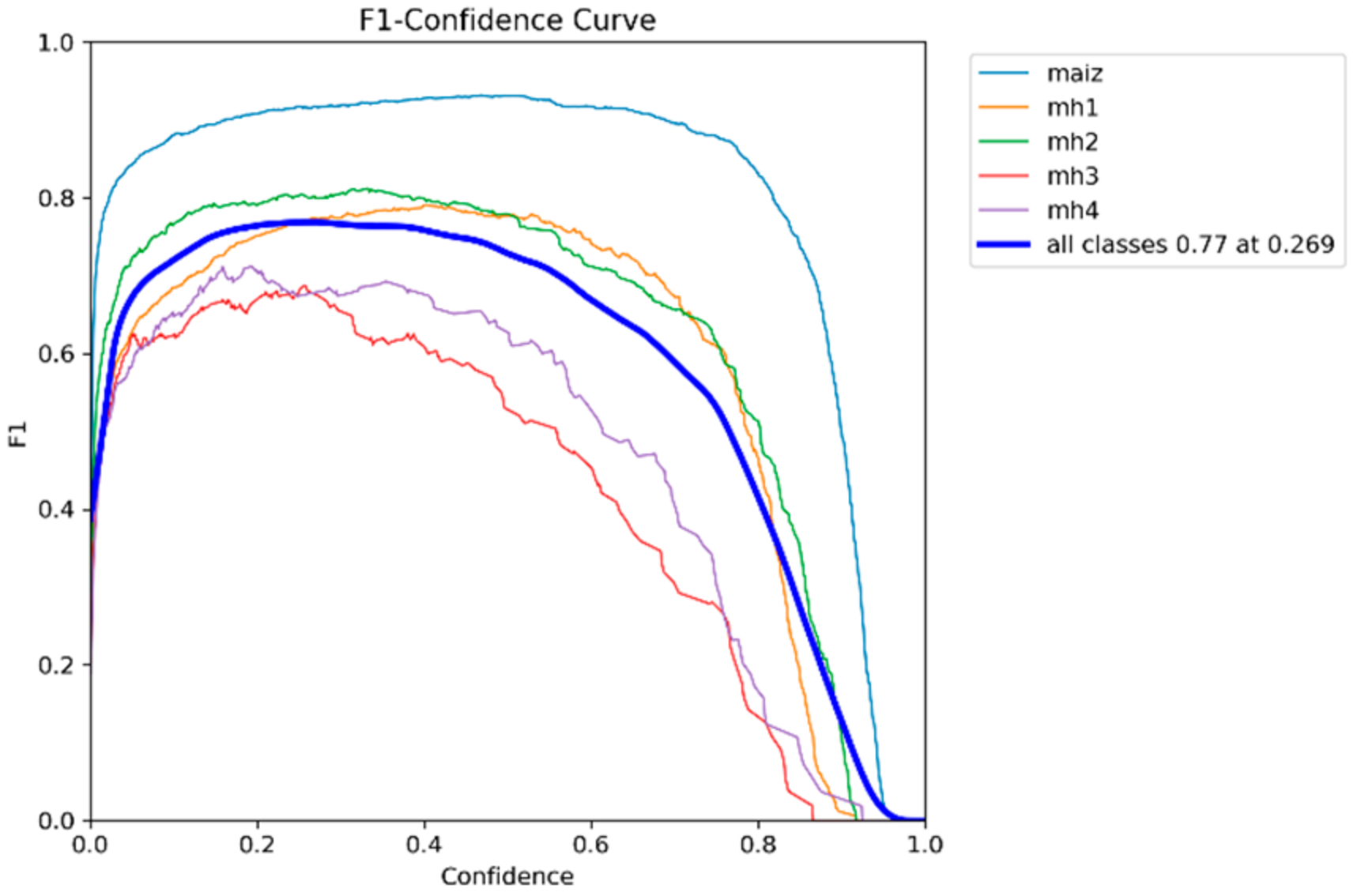
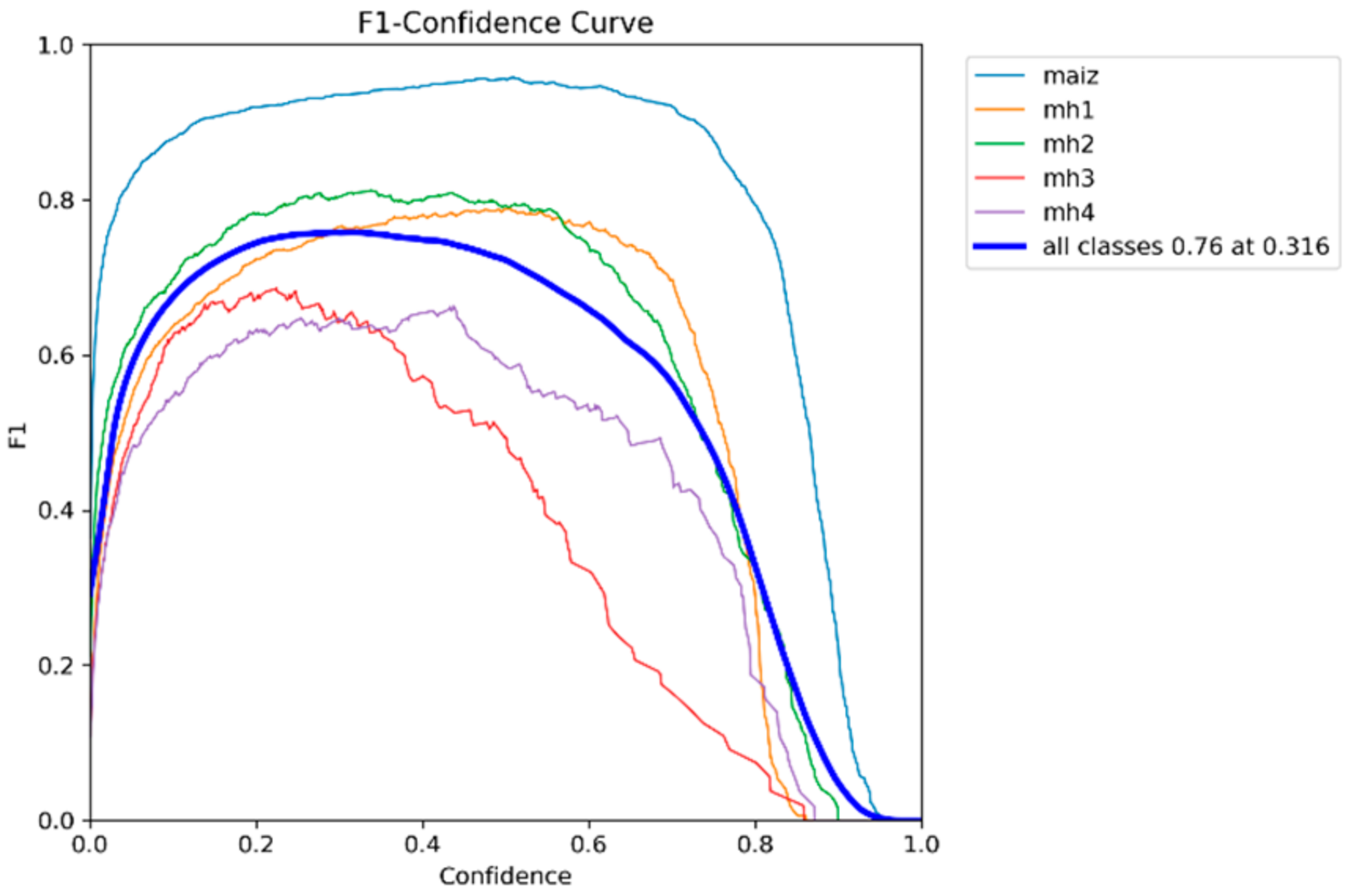
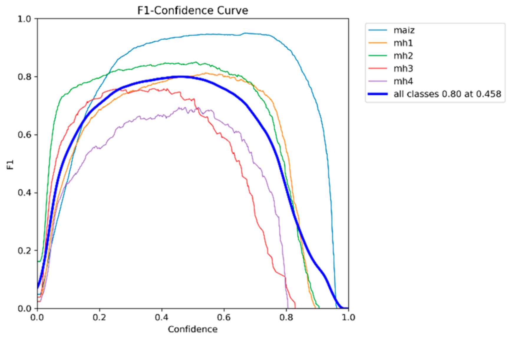
RT-DETR-l	0.80	0.458

shows F1-score values and corresponding balanced confidence thresholds for five models (YOLOv8s, YOLOv9s, YOLOv10s, YOLOv11s, and RT-DETR-L). These values were calculated from the F1-score–Confidence curves and reflect the optimal balance between accuracy and recall for each model.

According to Table 4, the YOLOv8s model with an F1-score of 0.78 achieves a good balance between accuracy and recall with a relatively high confidence threshold of 0.400. This indicates that the model tends to be more conservative in its predictions, focusing on reducing false positives while maintaining a competitive F1-score. The YOLOv9s model has the same F1-score as the 0.78 YOLOv8s but with a significantly lower confidence threshold of 0.280; this suggests that the model is more aggressive in detecting positives. As for the YOLOv10s model, the slightly lower 0.77 F1-score reflects a drop in the balance between accuracy and recall compared to YOLOv8s and YOLOv9s. The lower confidence threshold of 0.269 indicates that this model prioritizes recall over accuracy. The YOLOv11s model has the lowest F1-score among the evaluated 0.76 models, indicating a lower overall balance between accuracy and recall. The intermediate confidence threshold of 0.316 reflects that the model is more moderate in its selectivity compared to YOLOv9s and YOLOv10s. The RT-DETR-l model is of higher overall performance, reaching the highest F1-score of 0.80, and its confidence threshold is higher than 0.458, suggesting that this model is more conservative, maintaining a good overall balance, but at the cost of having higher false positives.

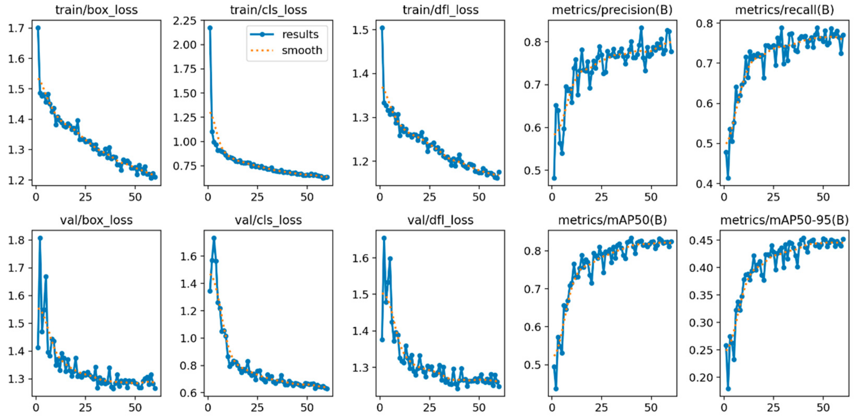
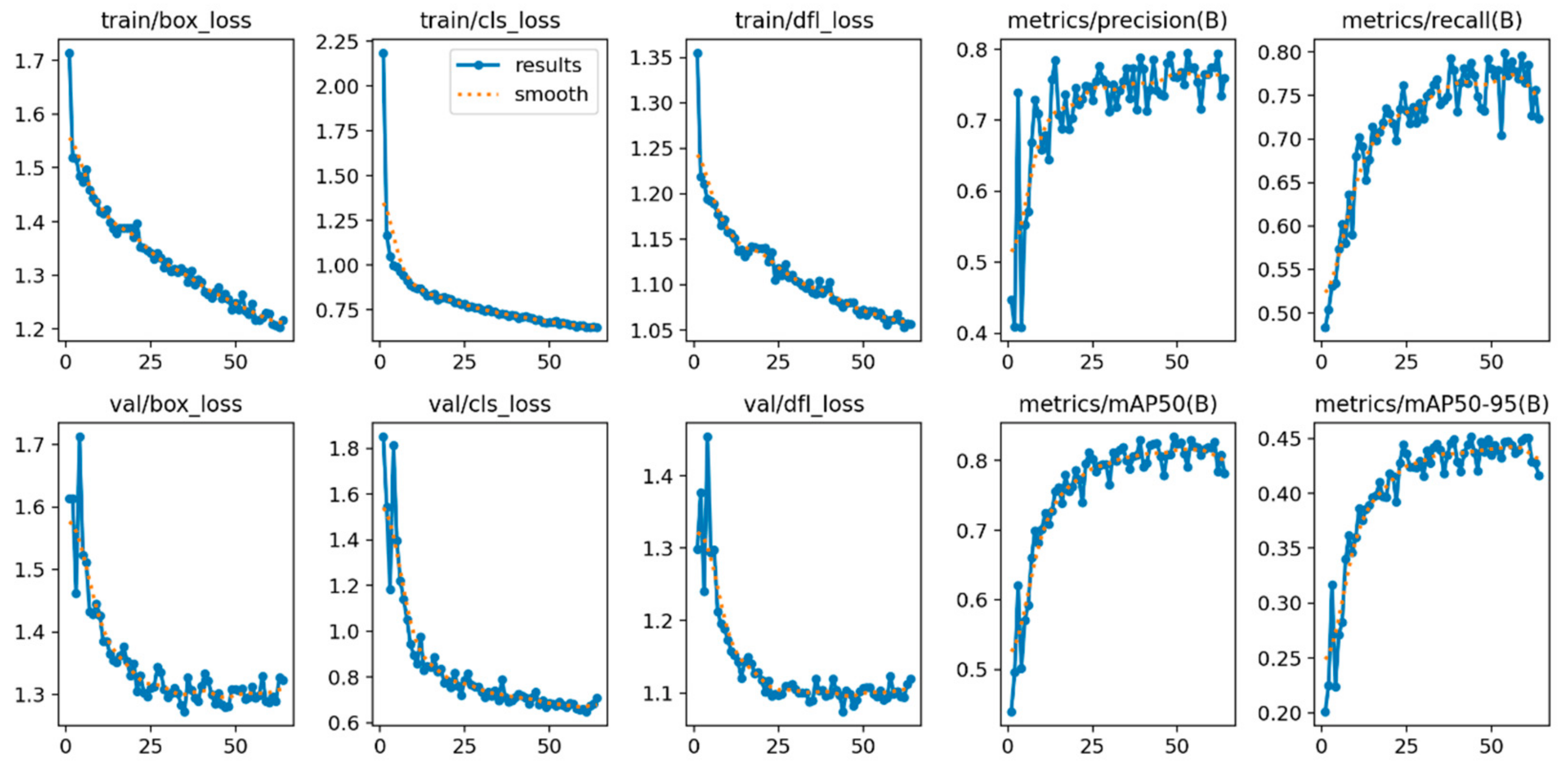
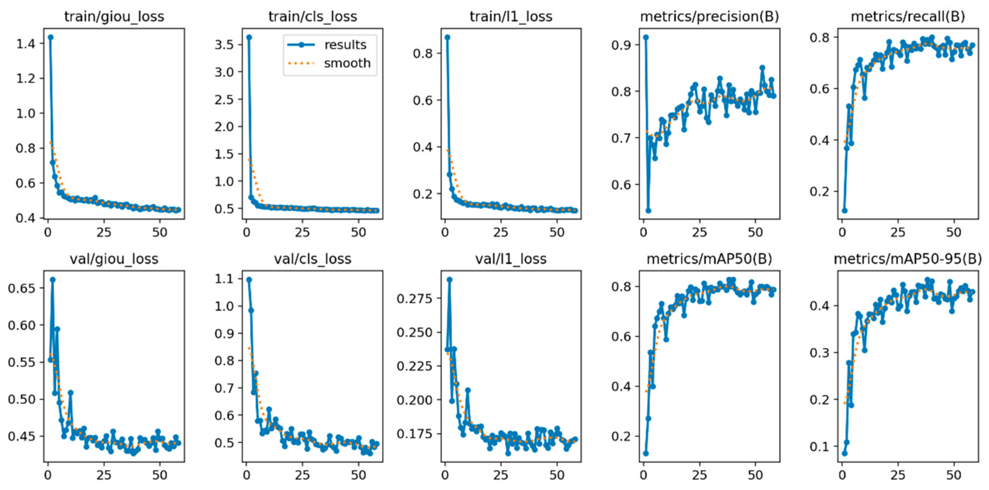
3.4. Evolution of Losses and Metrics During Training and Validation of the YOLOv8s, YOLOv9s, YOLOv10s, YOLOv11s, and RT-DETR-L Models

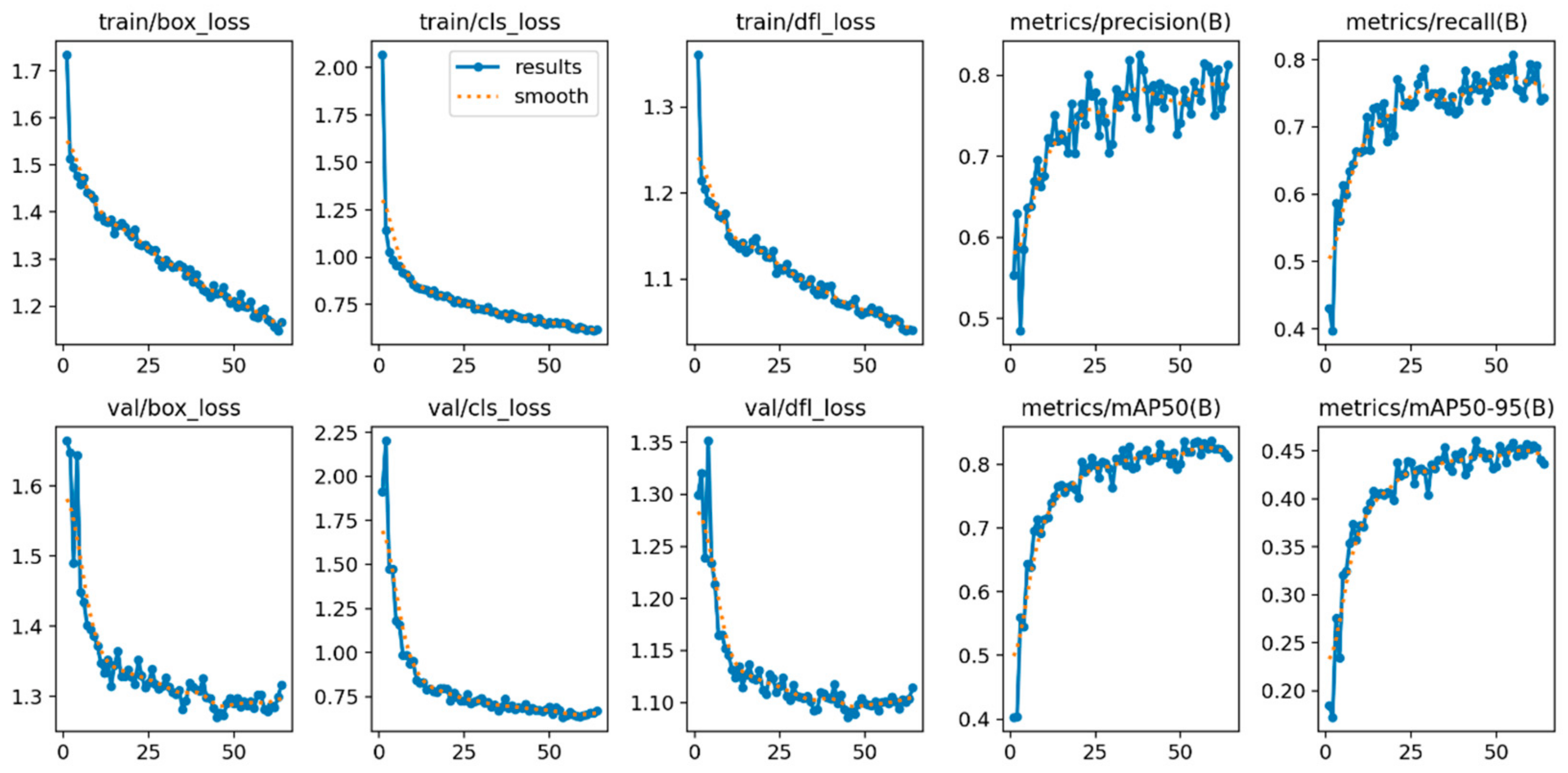
For the analysis of the evolution of losses and metrics,

Table 5. Number of times where the models converge.

MODEL	YOLOv8s	YOLOv9s	YOLOv10s	YOLOv11s	RT-DETR-l
Epochs	64	60	87	64	58

was constructed, which shows the number of times each model is required to achieve convergence during training. Convergence is defined as the point where losses (losses) and key metrics (precision, recall, and mAP) stop improving significantly, indicating that the model has learned the main patterns of the dataset.

RT-DETR-l and YOLOv9s are the fastest, converging in 58 and 60 epochs, respectively, making them ideal for efficient workouts. The YOLOv8s and YOLOv11s models require 64 epochs, striking a balance between time and learning. On the other hand, YOLOv10s needs 87 epochs, being the slowest model to converge; this does not mean that it is less efficient than the others. Additionally, Figure 25, Figure 26, Figure 27, Figure 28 and Figure 29 were constructed in which the behavior of losses (box_loss, cls_loss, and dfl_loss) and key metrics (precision, recall, mAP@0.5, and mAP@0.5–0.95) are shown during training and validation for each model analyzed.

The Box Loss evaluates the discrepancy between predicted and actual bounding boxes, adjusting parameters to optimize the position, size, and shape of these boxes using metrics such as IoU. The Cls Loss (cls_loss) measures the accuracy in classifying detected objects to ensure that each bounding box is correctly associated with its corresponding category. On the other hand, the DFL Loss (Distribution Focal Loss—dfl_loss) refines the prediction of the coordinates of the bounding boxes by representing the locations as discretized distributions, improving accuracy in scenarios that demand high resolution or greater detail.

Figure 25 corresponds to the YOLOv8s model, which shows a rapid convergence of loss functions (box_loss, cls_loss, and dfl_loss), indicating efficient learning during the training process. The model reaches its maximum performance with a mAP@0.5 of 0.831 in epoch 44 and a mAP@0.5–0.95 of 0.460. Although the model was trained up to epoch 64, as shown in Table 5, the Early Stopping technique was implemented, which automatically stops the training when no improvement in the loss of the validation set is observed for a consecutive number of epochs this through the patience parameter, which in this case was set to 20 epochs.

In Figure 26, the YOLOv9s model achieves convergence over 60 epochs, with low losses and robust metrics demonstrating a solid balance between accuracy and recall. Its maximum performance in mAP@0.5 of 0.834 is reached in epoch 40, standing out for an outstanding performance for standard detections. As for all the models, the Early Stopping technique was used to configure the patience parameter in 20 epochs; the mAP@0.5–0.95 achieved a value of 0.454, which suggests room for improvement in more accurate detections.

Figure 27 shows that the YOLOv10s model converges at epoch 87, evidencing robust performance with a mAP@0.5 of 0.831. Reduced and stable losses throughout training indicate that the model is properly adjusted. In addition, it achieves a mAP@0.5–0.95 of 0.456, reinforcing its overall performance; the Early Stopping technique was used to configure the patience parameter in 20 epochs.

In Figure 28, the YOLOv11s model achieves convergence in 64 epochs and achieves robust performance with a mAP@0.5 of 0.824 and a mAP@0.5–0.95 of 0.452. The consistent losses between training and validation reflect a generalized model, likewise, the Early Stopping technique was implemented with the patience parameter set in 20 epochs.

In Figure 29, it can be observed that the RT-DETR-l model converges at epoch 58, which shows a high efficiency in the training process and a robust performance, reaching a mAP@0.5 of 0.828 and a mAP@0.5–0.95 of 0.456. The stability and low level of losses during training reflect a well-adjusted model. For this training, the Early Stopping technique was implemented, configuring the patience parameter in 20 epochs to automatically stop the process in the absence of improvements in the validation set.

3.5. Diagnosis and Comparison of Models YOLOv8s, YOLOv9s, YOLOv10s, YOLOv11s, and RT-DETR-L

The trained and analyzed models, YOLOv8s, YOLOv9s, YOLOv10s, YOLOv11s, and RT-DETR-l, generally meet the objective of detecting maize and the four types of weeds. However, there is a difference between them that makes them stand out more than others in their efficiency, balance, and overall performance, as shown in

Table 6. Summary of global metrics obtained from each model.

MODELs	Precision	Recall	mAP@0.5	mAP@0.5–0.95	F1-Score	Confidence Threshold
YOLOv8s	0.790	0.777	0.831	0.460	0.78	0.4
YOLOv9s	0.801	0.765	0.834	0.454	0.78	0.28
YOLOv10s	0.789	0.760	0.831	0.456	0.77	0.269
YOLOv11s	0.742	0.787	0.825	0.452	0.76	0.316
RT-DETR-l	0.814	0.791	0.828	0.456	0.8	0.458

.

According to the values in Table 6, it is possible to determine which models are most suitable for the purpose of this study. For this purpose, the value of mAP@0.5 is first considered as the primary evaluation criterion since a high value in this metric indicates that the model is able to correctly detect objects with a minimum of 50% overlap (IoU) between the prediction and the real object. Secondly, the F1-score, which reflects the balance between accuracy and recall, was analyzed. A high value in this metric ensures that the model achieves an optimal balance between correct object identification and error minimization, reducing both FP and FN. Thus, the combination of a high mAP@0.5 with a robust F1-score allows the selection of the most efficient and reliable model for object detection in this study. Based on these criteria, the models that obtained the best results were the YOLOv9s model and the RT-DETR-l model.

The YOLOv9s model stands out for leading in the overall average, achieving a mAP@0.5 of 0.834 and a mAP@0.5–0.95 of 0.454, which reflects a high detection capacity in diverse scenarios. In terms of balance, it obtained an F1-score of 0.78, evidencing an adequate balance between an overall precision of 0.801 and an overall recall of 0.765, although its relatively low confidence threshold of 0.280 suggests that the model is more permissive, accepting predictions with lower probability. In terms of accuracy per class, YOLOv9s showed outstanding results: the “maize” class reached 0.909, followed by “mh2” with 0.893, “mh1” with 0.779, “mh3” with 0.810, and “mh4” with 0.636, consolidating its performance as robust in several categories. Its convergence is at 60 epochs, making it competitive in speed and performance.

The RT-DETR-l model stands out for obtaining a higher overall performance, reaching the highest F1-score of 0.80. Its confidence threshold is higher than 0.458, which suggests that this model is more conservative, with an overall precision of 0.814 and an overall recall of 0. 791, maintaining a good overall balance, but at the cost of having greater false positives, which is reflected in the precision per class. For the “maize” class, it obtained 0.754, for the “mh1” class 0.638, “mh2” 0.805, “mh3” 0.798, and for the “mh4” 0.497, which is lower than for the YOLOv9s model. Regarding recall per class, the RT-DETR-l model obtained higher values compared to YOLOv9s, especially in the more challenging classes “mh3” and “mh4”, which makes it interesting since in these classes, the YOLO models presented lower yields. Additionally, the RT-DETR model was the fastest to complete its training by converging in 58 epochs.

Although the other YOLOv8s, YOLOv10s, and YOLOv11s models show a solid performance in terms of overall metrics, they do not excel in the classification of more challenging weeds, with classes “mh3” and “mh4” being surpassed by the YOLOv9s model. However, we analyzed their performance.

Comparing YOLOv8s with YOLOv9s, it was observed that YOLOv9s demonstrates superior performance compared to YOLOv8s, excelling in all key metrics. Its precision is 0.801 vs. 0.790, and its mAP@0.5 of 0.834 vs. 0.831 is higher, indicating a greater ability to detect objects accurately. Although both models share the same F1-score of 0.78, YOLOv9s has a lower confidence threshold of 0.28 vs. 0.4, allowing it to perform more detections without being overly restrictive. This factor makes it more efficient in situations where a trade-off between detection and prediction confidence is required. However, when comparing YOLOv8s to RT-DETR-l, the latter outperforms in all key metrics, with a higher precision of 0.814 vs. 0.790 and a higher recall of 0.791 vs. 0.777, indicating that RT-DETR-l detects more objects with lower error rate. In addition, its F1-score of 0.8 vs. 0.78 reinforces its better overall balance between precision and recall.

As for YOLOv10s, its performance is slightly inferior to YOLOv9s in several key aspects. YOLOv10s precision of 0.789 and its mAP@0.5 of 0.831 are lower compared to those of YOLOv9s, indicating that it has a lower detection capability. In addition, its F1-score of 0.77 vs. 0.78 in YOLOv9s reflects a less efficient balance between precision and recall. A relevant aspect is its lower confidence threshold of 0.269 vs. 0.28 in YOLOv9s, suggesting that it accepts more detections with lower certainty, increasing the risk of FP and affecting the reliability of predictions. In comparison with RT-DETR-l, YOLOv10s is also at a disadvantage, as RT-DETR-l has a higher precision of 0.814 vs. 0.789, a better recall of 0.791 vs. 0.760, and a higher F1-score of 0.8 vs. 0.77, making it more balanced and reliable. In addition, its mAP@0.5–0.95 of 0.456 in both models suggests that RT-DETR-l is equally efficient over a wide IoU range but with higher robustness in detection.

On the other hand, YOLOv11s differs by its higher precision of 0.787 vs. 0.765 in YOLOv9s, indicating that it is more efficient in detecting a larger number of objects. However, this advantage is accompanied by a reduction in precision of 0.742 vs. 0.801 in YOLOv9s, which generates a higher number of false positives. Its mAP@0.5 of 0.825 is the lowest among the YOLO models evaluated, and its F1-score of 0.76 vs. 0.78 in YOLOv9s confirms that its balance between precision and recall is less efficient. Moreover, its higher confidence threshold of 0.316 vs. 0.28 in YOLOv9s causes it to discard more detections, although it still maintains a higher false positive rate. Compared to RT-DETR-l, YOLOv11s is inferior in the precision of 0.742 vs. 0.814, recall of 0.787 vs. 0.791, and F1-score of 0.76 vs. 0.8, indicating that RT-DETR-l offers better overall performance with a better balance between detection and precision. Although YOLOv11s manages to detect more objects than other YOLO models, RT-DETR-l is still the most reliable and stable option in terms of overall performance.

Numerous studies have explored and compared different models of CNNs for weed detection in maize crops. For example, previous research has developed and evaluated various architectures with the aim of improving accuracy and efficiency in weed identification, optimizing existing models, and proposing new variants adapted to this specific context; for example, the authors of [38] designed a CNN based on the YOLOv4-tiny model to detect weeds in maize crop. To verify its effectiveness, it was compared with CNNs obtaining a mAP in Faster R-CNN and obtained a value of 0.685, 0.692 for SSD300, 0.855 for YOLOv3, 0.757 for YOLOv3-tiny, and 0.833 for YOLOv4-tiny; the proposed model obtained a value of 0.867. For the models analyzed in this study, their mAPs are lower for YOLOv9s with 0.834 and RT-DETR with 0.828, which does not mean that they are less efficient; it is necessary to take into account that the training set in [34] used five weed species but considered them as a single class, unlike our study that worked with four weed species.

In the work in [39], a precision spraying robot for maize crops based on YOLOv5s was developed. To evaluate its performance, different versions of the model were compared, including YOLOv5s, YOLOv5m, YOLOv5l, and YOLOv5x. The best configuration was a modification of YOLOv5s, which incorporated a C3-Ghost-bottleneck module, significantly improving the architecture. As a result, the optimized model achieved a mAP of 0.963 in maize detection and a mAP of 0.889 in weed detection, outperforming the standard versions in terms of accuracy and efficiency. The improved model is close to the results of this research, which for the maize class, the RT-DETR-l model obtained a 0.98 accuracy and YOLOv9s obtained an accuracy of 0.97; it is necessary to take into account that the authors of [39] only used one weed species “Solanum rostratum”, while in this study, four different species were evaluated. Likewise, the authors of [40] evaluated the behavior of YOLOv5s in the detection of weeds in the maize crop, obtaining excellent results in the global mAP@0.5, obtaining a value of 0.836. In the maize class, they achieved a mAP of 0.97, which is a result very similar to those obtained in this study, which shows that the YOLO models are suitable for detecting weeds in maize crops. On the other hand, in the study in [50], different versions of the YOLOv5 model (n, s, m, l, and x) were evaluated for the identification of four types of weeds in maize crops. The best results were obtained with YOLOv5l with a mAP@0.5 of 0.744 and YOLOv5x with a mAP@0.5 of 0.758. In addition, F1-score values ranged from 0.72 to 0.74, and confidence thresholds were in the range of 0.312 to 0.433. In comparison, YOLOv9s showed superior performance, reaching a mAP@0.5 of 0.834, indicating higher detection accuracy. Its F1-score of 0.78 was higher than that of YOLOv5, evidencing a better balance between precision and recall, with a lower false positive and false negative rate. In addition, its confidence threshold (0.28) is lower than that of YOLOv5, allowing for more flexible detection without compromising reliability.

The authors of [51] proposed an improved weed detection model based on YOLOv5s in maize fields with straw cover; for the selection of YOLOv5s, they evaluated several models obtaining a mAP value in Faster R-CNN of 0.719, SSD of 0.883, YOLOv4 of 0.922, YOLOv5s of 0.923, and YOLOv8 of 0.91. The proposed model faced several challenges in terms of variability in lighting, plant overlap, and environmental conditions. These variations affected the accuracy of the model, causing the mAP to decrease by 0.9%, as some weeds were partially hidden or confused with crop residues. Additionally, the model showed difficulties when facing new types of weeds not represented in the training set, which evidenced the need to increase the diversity of the dataset.

3.6. Inference of the YOLOv9s and RT-DETR-l Models

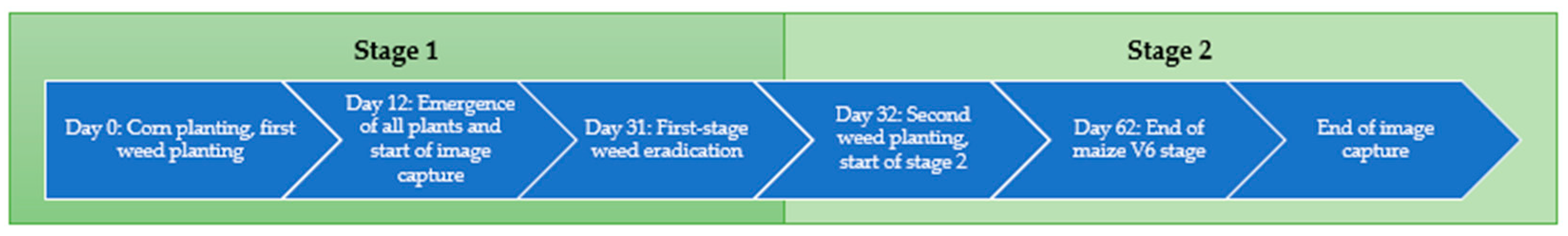
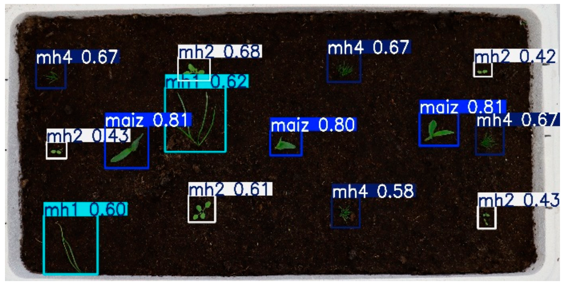
To verify the predictions of the top-performing models, inference was performed on images at two different stages of crop development, 15 and 30 days after planting. Each bounding box has its corresponding label and the probability value assigned by the model to detect the class.

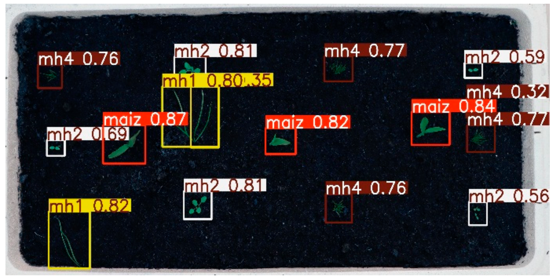
Figure 30 shows the inference of the YOLOv9s model on an image 15 days after planting. It can be observed that the model identified all the maize plants with probabilities of 0.81, 0.80, and 0.81. As for the weed “mh1”, it finds it twice, with probabilities of 0.60 and 0.62. The weed “mh2” was found five times, with probabilities ranging from 0.42 to 0.68. The model does not identify “mh3” weeds at this growth stage, although they exist in the image, and it confuses them with “mh2” plants, which is logical since in the early stages of growth, the weeds corresponding to “mh2” and “mh3” are similar as they are broad-leaved. As for the “mh4” weeds, it finds them four times with probabilities between 0.58 and 0.67.

Figure 31 corresponds to the inference of the RT-DETR-l model in an image 15 days after planting; it is observed that the model identified all the maize plants with probabilities of 0.87, 0.82, and 0.84. As for the weed “mh1”, the RT DETR-l model detects it three times, unlike YOLOv9s. One of the detections of the “mh1”, the RT-DETR-l model divides it into two distinct objects, which, for the purposes of our study, we do not consider an error; on the contrary, t is a success in identifying them separately, the probability of these is 0.80 and 0.35. Like YOLOv9s, the “mh2” weed was identified five times, with probabilities ranging from 0.56 to 0.81. As for the “mh3” weeds, the model did not identify any, just like YOLOv9s. As for the “mh4” weeds, the RT DERT-l model finds five with probabilities between 0.32 and 0.77, finding one more weed than YOLOv9s, which was correctly identified.

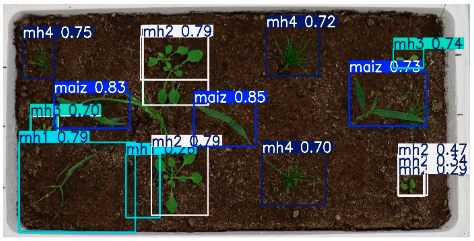
Figure 32 corresponds to the inference of YOLOv9s 30 days after planting; at this stage of growth, weeds are at a size that begins to compete strongly with maize plants. As for the maize plants, the three plants were identified with probabilities of 0.83, 0.85, and 0.73. Regarding the “mh1” weeds, two are identified, but one is new with respect to the previous image, and the other is not identified. The “mh2” weed was found five times; at this stage, the model does identify all the weeds present in this class and is no longer confused with the “mh3” weeds. As for the “mh3” weeds, two are identified with probabilities of 0.70 and 0.74. The “mh4” weeds were found four times, which is one time less than in the last stage; this is due to the fact that they were found under the maize plant.

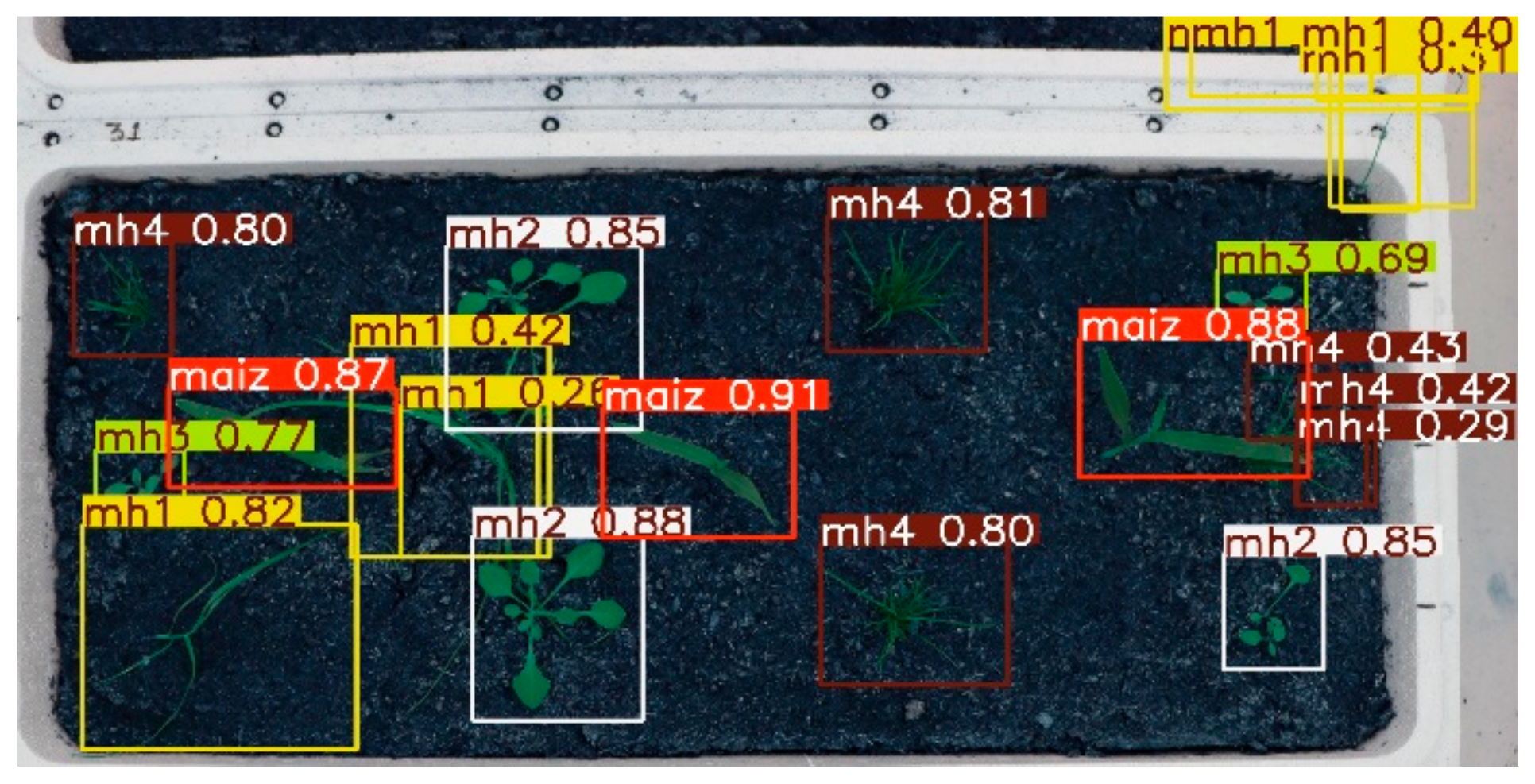
Figure 33 corresponds to the inference of RT-DETR-l 30 days after planting; the model finds the three maize plants with probabilities of 0.87, 0.91, and 0.88. In the case of the “mh1” weed, seven instances were detected, unlike the YOLOv9s model. RT-DETR-l managed to retain the identification of one instance that YOLOv9s did not recognize, and also detected one weed of this class that was in the early stages of growth. In addition, it found a weed of this class that was in the early stages of growth. Regarding the “mh2” weed, the model identified three of them, but in fact, there are five; the model joined two of the weeds into a single classification. As with the YOLOv9s model, the “mh3” weed was correctly detected twice. As for the “mh4” weed, this model identified six instances, an increase of two detections over YOLOv9s. These additional detections correspond to weeds partially hidden behind a corn plant.

These inferences visually show that despite their differences, the two models efficiently identify the weeds and differentiate them from the maize plants, making both models suitable for implementation in precision weeding systems.

4. Conclusions

The models YOLOv8s, YOLOv9s, YOLOv10s, YOLOv11s, and RT-DETR-l were trained for the detection of weeds in the cultivation of sweet corn Zea maiz L., for which four types of weeds, Lolium rigidum “mh1”, Sonchus oleraceus “mh2”, Saolanun nigrum “mh3”, and Poa annua “mh4”, were used. The results show that all models demonstrated outstanding performance in the identification of the “maize” class, suggesting that the morphological and visual characteristics of the crop are highly distinguishable from weeds, which is the purpose of this study, to differentiate maize plants from weeds. The YOLOv9s and RT-DETR-l models were the best performers in the yield analysis.

The YOLOv9s model demonstrated competitive performance, standing out in global metrics such as a mAP@0.5 of 0.834 and a mAP@0.5–0.95 of 0.454, indicating a high detection capability in different scenarios. Its F1-score of 0.78 reflects an adequate balance between precision and recall, although its low confidence threshold of 0.280 makes it more permissive, increasing detection sensitivity. In addition, the YOLOv9s model presented an outstanding performance in key categories, reaching an accuracy of 0.909 in “maize” and 0.893 in “mh2”, distinguishing itself as an efficient model with fast convergence in 60 epochs.

On the other hand, RT-DETR-l was positioned as the model with the best balance between precision and recall, reaching the highest F1-score of 0.80. Its higher confidence threshold of 0.458 makes it more conservative, although it generates more false positives in classes such as “maize” and “mh1” compared to YOLOv9s. However, it excels in recall, especially in challenging classes such as “mh3” and “mh4”, where it outperforms the YOLO models.

As for the other models, the YOLOv8s, YOLOv10s, and YOLOv11s models showed solid performances with mAP@0.5 values between 0.824 and 0.831, but with less balance between accuracy and recall. In this study, YOLOv9s was found to be the most suitable option, as it offers the optimal performance required for the implementation of an automatic weed detection system in maize crops.

In future work, Data Augmentation techniques will be integrated to increase the number of samples in the less represented and unbalanced classes, with the objective of improving performance in the categories that obtained insufficient results. Additionally, different models such as YOLO-NAS and PP-YOLOe will be evaluated, as well as modern architectures such as EfficientDet and DETR modifications, to analyze their effectiveness in detecting weeds in maize crops. New images of new campaigns, taken in various field conditions and phenological states and captured with different devices, such as drones and cameras mounted on agricultural machinery, will also be incorporated. This will make it possible to strengthen the models of trained CNNs, selecting the best CNN to integrate it into a highly efficient precision weeding system capable of operating in harsh field environments and handling the variability inherent in the different agricultural production conditions.

The use of artificial intelligence in agriculture represents a transformative opportunity to improve the efficiency, productivity, and sustainability of the primary sector. However, its adoption faces key challenges, such as data collection and quality, high development and implementation costs, and the need for a regulatory framework that ensures the security, privacy, and accessibility of information, in addition to protecting farmers’ ancestral knowledge. Overcoming these limitations will be critical to maximizing the positive impact of AI in agriculture and ensuring its equitable and sustainable integration.

Integrating CNN models with machine vision systems opens up a broad spectrum of applications beyond the scope of this work, which focuses on evaluating different CNN models that can be integrated into a precision weeding system capable of selective and high-precision weed removal. These systems could also incorporate algorithms designed to monitor the state of crops, maintaining a constant record of their growth. In addition, this technology can be used to monitor damage caused by pests or diseases, facilitating timely decision-making on preventive or corrective measures.

The long-term effectiveness of precision weeding is reflected in three key aspects: crop yield, profitability, and environmental impact. By reducing weed competition in a selective and localized manner, crops can optimally access essential resources, resulting in higher yields and improved end-product quality. From an economic standpoint, precise herbicide application lowers the costs associated with chemical inputs and reduces the need for manual interventions, improving the profitability of agricultural production. In addition, this approach minimizes the indiscriminate use of herbicides, which contributes to the reduction in weed resistance to chemicals, promoting more sustainable agricultural practices. In environmental terms, the localized application of herbicides reduces soil and water pollution, reduces the ecological footprint of agricultural production, and favors the preservation of biodiversity in agricultural ecosystems. In this way, precision weeding not only optimizes productivity and costs in the short term but also establishes a basis for more efficient, profitable, and sustainable agriculture in the long term.

The incorporation of new algorithms, adapted and trained specifically for each type of crop, represents an interesting line of future research. In the context of precision weeding, CNN models could be combined with innovative technologies that remove weeds without resorting to agrochemicals. For example, pressurized water jet systems could be integrated to cut weeds or laser technologies for their removal, promoting cleaner agriculture. This approach not only drives the modernization of agricultural tools but also contributes to more efficient and sustainable crop management, marking a significant advance in precision agriculture.