Integrating UAV-Based Multispectral Data and Transfer Learning for Soil Moisture Prediction in the Black Soil Region of Northeast China

Abstract

The rapid and accurate acquisition of soil moisture (SM) information is essential. Although Unmanned Aerial Vehicle (UAV) remote sensing technology has made significant advancements in SM monitoring, existing studies predominantly focus on developing models tailored to specific regions. The transferability of these models across different regions remains a considerable challenge. Therefore, this study proposes a transfer learning-based framework, using two representative small agricultural watersheds (Hongxing region and Woniutu region) in Northeast China as case studies. This framework involves pre-training a model on a source domain and fine-tuning it with a limited set of target domain samples to achieve high-precision SM inversion. This study evaluates the performance of three algorithms: Random Forest (RF), Convolutional Neural Network (CNN), and Long Short-Term Memory (LSTM) network. Results show that the fine-tuned model significantly mitigates the decline in prediction accuracy caused by regional differences. The fine-tuned LSTM model achieved the highest retrieval accuracy, with the following results: 10% samples (R = 0.615, RRMSE = 15.583%), 30% samples (R = 0.682, RRMSE = 13.97%), and 50% samples (R = 0.767, RRMSE = 16.321%). Among these models, the LSTM model exhibited the most significant performance improvement and the best transferability. This study underscores the potential of transfer learning for enhancing cross-regional SM monitoring and providing valuable insights for future UAV-based SM monitoring.

1. Introduction

Soil moisture (SM) is a critical driver in terrestrial hydrological and ecological cycles [1]. In-depth research on the dynamic variation in SM is essential for water resource management, soil conservation, as well as drought risk assessment and early warning [2,3]. Small agriculture watersheds, characterized by their unique hydrogeological features, serve as ideal sites for studying SM variations [4]. Traditional SM measurement methods, such as field sampling and laboratory SM testing [5], provide highly accurate point-based data. However, these methods face challenges in obtaining large-scale, high-frequency SM data due to spatial extent limitations and monitoring frequency constraints [6]. Additionally, they are constrained by high costs and spatiotemporal limitations [7], making it particularly difficult to capture SM variations at larger scales, especially in areas with diverse land use types [8,9,10,11]. Satellite remote sensing technology has demonstrated significant advantages in regional-scale soil moisture assessments through platforms like SMAP (Soil Moisture Active Passive) and SMOS (Soil Moisture and Ocean Salinity), which provide extensive coverage and multidimensional data support specifically for soil moisture retrieval. However, these remote sensing products typically have coarse spatial resolutions on the order of tens of kilometers [12], limiting their ability to capture surface-level details, especially in complex terrains or diverse land use areas. Moreover, while optical remote sensing data provide high spatial resolution, they are often limited by revisit cycles and weather conditions, reducing their suitability for real-time monitoring of rapidly changing processes [13].

Recent advancements in Unmanned Aerial Vehicle (UAV) remote sensing technology have provided unprecedented opportunities to address the aforementioned challenges. With their excellent mobility and capability to rapidly acquire high-resolution data, UAVs offer an efficient and reliable means for monitoring and assessing SM. In recent years, UAV remote sensing technology has been extensively applied to field-scale SM studies [14,15]. Additionally, the integration of machine learning and deep learning techniques for SM inversion has gained increasing popularity. In this context, machine learning methods have emerged as powerful tools for processing remote sensing covariates and SM data [16]. Random Forest (RF), a robust non-parametric ensemble learning method, can effectively capture the nonlinear relationships between SM and environmental variables [17], making it particularly suitable for addressing feature importance issues when using multispectral data from UAVs along with ground-measured data. Chen et al. [18] conducted a detailed monitoring study on summer maize at different growth stages by integrating the RF algorithm with the Particle Swarm Optimization–Support Vector Machine (PSO-SVM) model. Ground-truth data and multispectral imagery were gathered at six crop growth stages to serve as the dataset for developing a UAV-based spectral information framework aimed at soil moisture content (SMC) estimation. Two-thirds of the dataset was used for model training, while the remaining one-third was reserved for testing. Model performance was evaluated using the coefficient of determination (R²) and root mean square error (RMSE) as key metrics. The results indicated that these machine learning models performed exceptionally well during the jointing stage of maize; however, prediction accuracy gradually declined in subsequent growth stages. Notably, the RF model demonstrated strong robustness in SMC estimation, with R² values on the test set consistently exceeding 0.5 and, in some cases, surpassing 0.7. These findings highlight the stability and reliability of the RF model for soil moisture monitoring. Moreover, Zhang et al. [19] utilized UAV-based multispectral, thermal infrared, and RGB data and applied three machine learning algorithms—Partial Least Squares Regression (PLSR), K-Nearest Neighbors (KNNs), and RF—to predict SMC in maize fields under different irrigation levels. Their study was based on a dataset of 300 soil moisture samples collected from 2018 to 2019, which was divided into a training set and a test set in an 8:2 ratio to ensure model generalization. The results indicated that the RF algorithm outperformed the other models in SMC prediction, achieving coefficients of determination (R²) of 0.68 and 0.78 at soil depths of 10 cm and 20 cm, respectively. The relative root mean square errors (RRMSEs) were 20.82% and 19.36%, demonstrating high prediction accuracy. This study highlighted the significant potential of the RF algorithm for irrigation scheduling at the farmland scale.

With the rapid development of deep learning technology, its powerful predictive capabilities have made it a preferred method for remote sensing data analysis [20]. Convolutional Neural Networks (CNNs) and Long Short-Term Memory (LSTM) networks excel in spatial data interpretation and are particularly suited for predicting SM changes in response to land use variations. For instance, Hegazi et al. [21] proposed a novel non-contact soil moisture monitoring method based on a Convolutional Neural Network (CNN) framework. This framework consisted of six convolutional layers, one max-pooling layer, one flattened layer, and one fully connected layer for final prediction. The model utilized 17,325 Sentinel-1 satellite images and soil moisture data from the OZNET and WEGENERNET networks of the International Soil Moisture Network (ISMN) as data sources. During model training and evaluation, the dataset was divided into a training set and a test set in an 8:2 ratio to ensure its generalization capability. The coefficient of determination (R²), mean absolute error (MAE), and root mean square error (RMSE) were selected as evaluation metrics. The results showed that the model achieved an R² of 0.864, an MAE of 0.0144, and an RMSE of 0.0274, demonstrating the stability and accuracy of the predictions. Additionally, Ahmed et al. [22] developed an innovative soil moisture (SM) prediction framework, BRF-LSTM, by integrating a long short-term memory (LSTM) network with BRF feature selection techniques. This framework not only leveraged the strength of LSTM in handling time-series data but also incorporated the BRF feature selection method to enhance predictive performance. During model training, the dataset derived from Coupled Model Intercomparison Project Phase 5 (CMIP5) simulations was normalized and then divided into 70% historical data (1950–2005) for training and 30% for validation. Additionally, future soil moisture predictions (2006–2100) were utilized for independent testing to assess the model’s generalization capability. Evaluation results demonstrated that the BRF-LSTM framework outperformed standalone models in two different warming scenarios, with over 95% of prediction errors remaining below 0.02 mm and a relatively low root mean square error (RMSE), confirming the superiority of this framework in terms of prediction accuracy. These studies further highlight the broad application potential of deep learning models in predicting dynamic SM changes when combined with remote sensing data.

Although machine learning and deep learning technologies have made significant progress in field-scale SM inversion, research on shallow and deep SM prediction at the watershed scale, particularly in areas with complex land use types, remains underexplored. At the watershed scale, land use typically encompasses mixed types such as grassland, forest, farmland, and bare land, each exhibiting significantly different SM characteristics [23,24]. The diversity of terrains, land use practices, and soil types affects water storage and infiltration capacity, further complicating remote sensing-based SM inversion. The spatial heterogeneity of these landscapes makes accurate SM prediction even more challenging [25]. Meanwhile, applying different models across various geographic regions presents numerous challenges. Due to variations in terrain, climate, and land use, SM characteristics exhibit significant spatial heterogeneity across regions. Traditional machine learning and deep learning algorithms often rely on large, region-specific datasets, which are difficult to obtain in many areas. This dependence on data limits the spatial applicability of models. Additionally, transferring SM values between models may introduce errors, and model transferability is typically confined to the same geographic region [26,27].

Transfer learning offers an effective strategy to mitigate the heavy reliance on ground-truth data in traditional machine learning and deep learning models while overcoming data acquisition and model transfer limitations [28,29]. Transfer learning enables knowledge from data-rich regions to be transferred to data-scarce regions, allowing models trained in one region to be fine-tuned and applied in another without complete retraining. This approach not only compensates for data scarcity but also achieves high prediction accuracy [30,31], significantly enhancing the generalization ability and application efficiency of the models. Currently, transfer learning has been successfully applied in various fields, including land cover mapping [32], vegetation monitoring [33], soil property assessment [34], crop yield prediction [35], and water resource management [36]. However, studies combining UAV technology for cross-regional SM prediction remain relatively scarce.

Based on this, this study focuses on the application of transfer learning for soil moisture prediction across agricultural regions at different depths (0–10 cm, 20–30 cm, and 20–40 cm) and proposes a transfer learning framework for cross-regional SM inversion, using the small watersheds from the Hongxing (HX) and Woniutu (WNT) regions as research areas. This framework initially constructs a model utilizing source domain data from the HX region. Subsequently, it fine-tunes the pre-trained model using varying proportions of samples from the target domain (WNT) to evaluate both the model’s transferability and the fine-tuning ratio. Under this framework, UAV remote sensing data are combined with transfer learning techniques to improve soil moisture estimation accuracy across different regions and depths. The performance of RF, CNN, and LSTM algorithms is systematically evaluated. Specifically, key features such as the normalized difference vegetation index (NDVI) and the green normalized difference vegetation index (GNDVI) are first extracted from UAV imagery and correlated with ground-measured soil moisture data. During model training, the model is initially pre-trained on source domain data and then fine-tuned using a limited amount of target domain data to enhance its adaptability and predictive accuracy. The primary objective of this study is to enhance SM prediction in complex small watersheds by integrating UAV multispectral data with transfer learning. The specific goals and key contributions include the following: (1) developing a novel approach that combines UAV multispectral remote sensing with transfer learning to explore the potential of a transfer learning framework for SM inversion in small watersheds; (2) conducting a comprehensive comparison of RF, CNN, and LSTM models in terms of prediction accuracy, adaptability, and robustness across soil depths; and (3) evaluating the effectiveness and advantages of the transfer learning framework in cross-regional SM prediction and scenarios with limited target domain data.

2. Materials and Methods

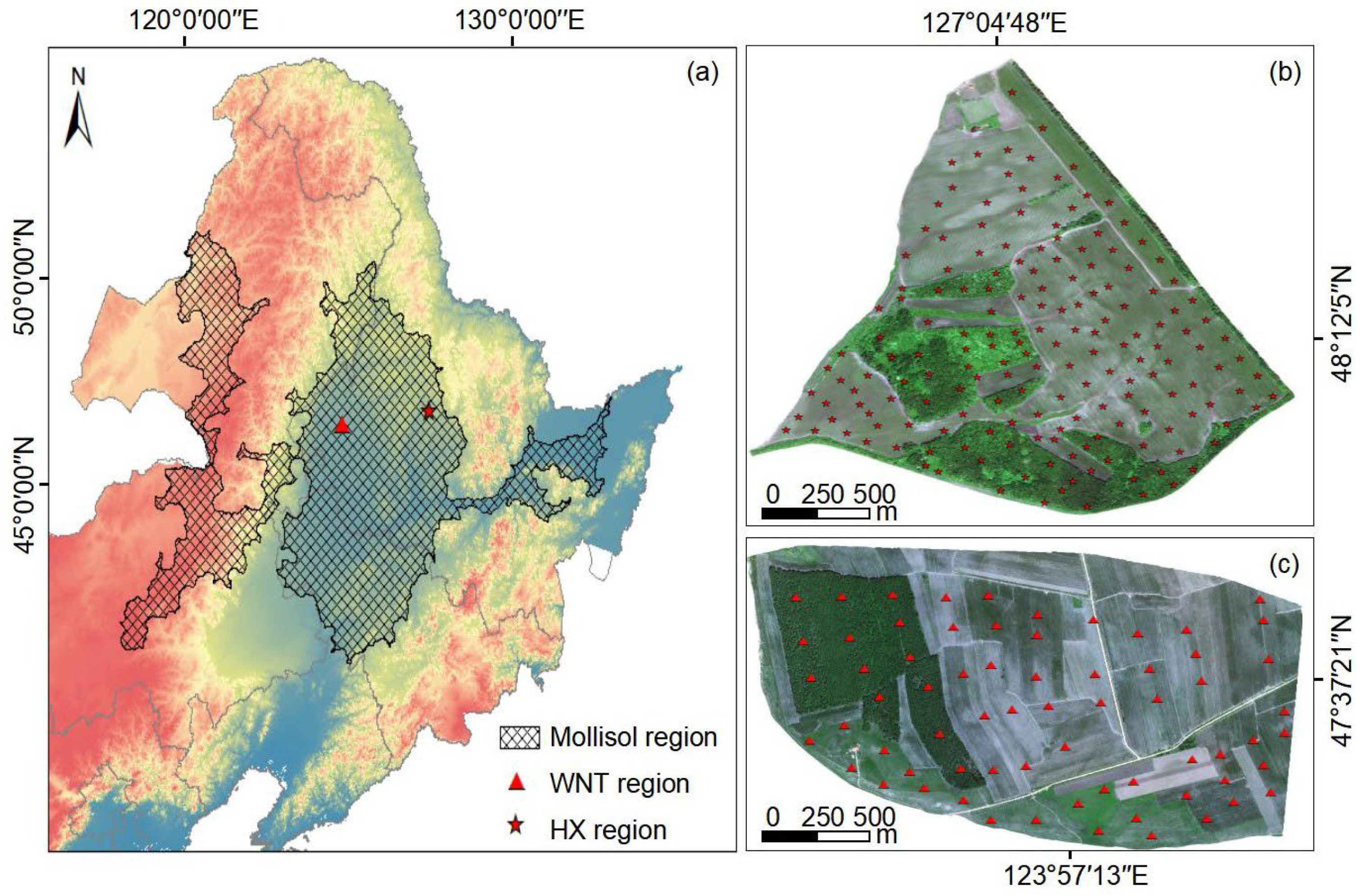
2.1. Study Area

This study selected two representative research areas in the black soil region of Northeastern China: the HX region and the WNT region (Figure 1a). Both regions are typical rain-fed agricultural areas, located approximately 350 km apart.

The HX region is situated in Beian City, Heilongjiang Province (48°21′ N, 126°08′ E) (Figure 1b), within the Mollisol region of Northern China. It experiences a temperate semi-humid continental monsoon climate, characterized by cold, dry winters and warm, rainy summers. The average annual precipitation is 555 mm, with a frost-free period of about 140 days. According to the Food and Agriculture Organization (FAO) classification (FAO, 2015 [37]), the primary soil type is referred to as “black soil” or “clayey soil.” The topography is gently sloping, with an average gradient of 5°. Land use is predominantly arable land [38], with small areas of natural forest and grassland, primarily formed by reclamation from forested areas.

The WNT region is located on the Songnen Plain (47°37′11″ N, 123°56′17″ E) (Figure 1c), part of the alluvial and fluvial plain of the Songhua River in Heilongjiang Province, Northeastern China. This region has a typical temperate continental monsoon climate, with an average annual precipitation of 433 mm and an average temperature of 3.2 °C. The frost-free period is approximately 130 days. The primary land use type is arable land, followed by natural grassland and forest. According to the FAO classification (FAO, 2015, [37]), the dominant soil type is “sandy black soil.” The terrain is also characterized by gentle slopes, with an average gradient of approximately 5° [39].

2.2. Data Sources

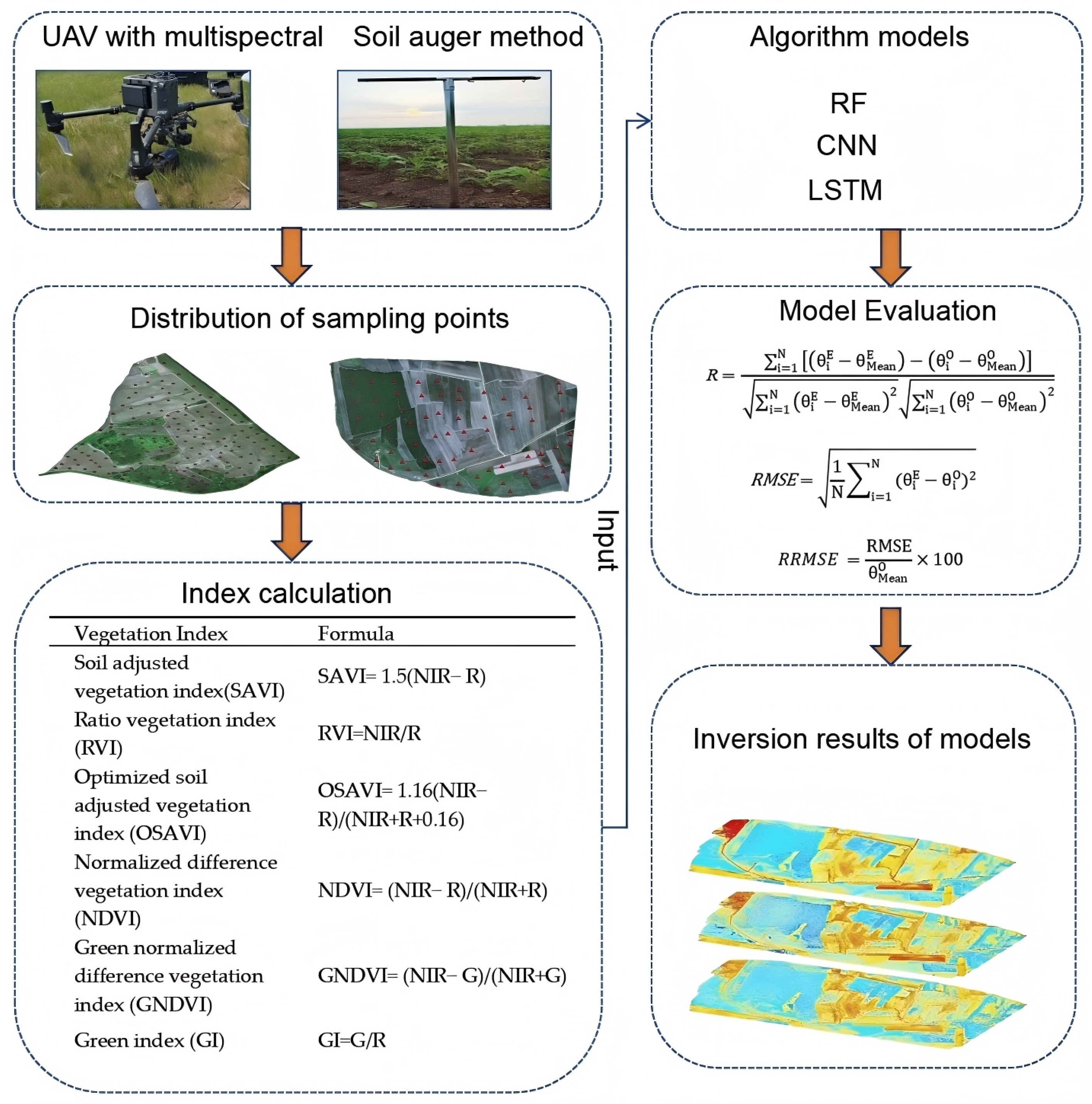
2.2.1. UAV Multispectral Data

Image acquisition was conducted using a DJI Matrice 300 drone (DJI Technology Co., Ltd., Shenzhen, China) equipped with the MS600 Pro multispectral camera (Changguang Yusense Co., Ltd., Qingdao, China). The MS600 Pro is a six-band multispectral camera installed on a stabilized platform to ensure smooth and clear images during each flight. The camera captures six spectral bands: blue (450 nm), green (555 nm), red (660 nm), red edge 1 (720 nm), red edge 2 (750 nm), and near-infrared (840 nm). All image data were accurately calibrated to convert them into orthorectified surface reflectance values. Data collection was scheduled between 11:00 AM and 2:00 PM under clear weather conditions to ensure the solar zenith angle was greater than 50°, thereby ensuring high-quality imagery. The flight parameters were set as follows: an altitude of 400 m, a flight speed of 5 m per second, and a vertical camera orientation with a focal length of 25 mm. The longitudinal overlap of the images was 85%, and the lateral overlap was 75%, ensuring a ground resolution of 20 cm per pixel. The calibration system included an optical intensity sensor and a fixed reflectance calibration panel for optical and radiometric corrections.

Image processing was performed using Pix4D Mapper software (version 4.5.6, Pix4D, Lausanne, Switzerland) to stitch the raw remote sensing data. ENVI 5.6 software was utilized for band fusion and radiometric correction. Subsequently, ArcMap 10.8 was employed to extract reflectance values at sampling points from the processed images. The collected reflectance data were then used to analyze the correlation with soil water content in agricultural crops.

Data for the WNT region were collected on 1 July 2024, while data for the HX region were collected on 2 July 2024. During these two days of image acquisition, the weather was clear and cloudless, providing optimal flight conditions and ensuring the accuracy and reliability of the UAV remote sensing data for both research areas.

2.2.2. In Situ SM

Since there are no publicly available datasets that meet the research requirements for these two study areas, we collected UAV data and ground-measured SM data in both regions to meet research requirements and ensure the accuracy of the soil moisture data and the effectiveness of transfer learning. With the UAV image acquisition, field SM sampling was simultaneously conducted in both the WNT region and HX region study areas; the sampling points are shown in Figure 1b,c. The sampling points were evenly distributed across the study areas, covering various land use types, including farmland, forest, grassland, and slopes. Soil samples were collected using the soil auger method at depths of 0–10 cm, 10–20 cm, and 20–40 cm. The collected black soil samples were placed in aluminum boxes. On the day of sampling, the wet weight of the samples was recorded, after which they were dried in an oven at 105 °C for 8 h. Once drying was complete, the dry weight of the soil was measured. The SM content (SMC) was calculated using the following formula:

$$\theta ={\displaystyle \frac{w-w’}{w’}}$$

(1)

where $\mathrm{w}$ is the wet weight of the sample and $\mathrm{w}\mathrm{’}$ is the dry weight of the sample.

In total, 519 in situ SM samples were collected from the HX region, with 173 samples from each soil depth layer, and 210 in situ SM samples were collected from the WNT region, with 70 samples from each depth layer. Soil and elevation information of the two study regions are presented in

Table 1. Soil texture and elevation in the HX region and the WNT region.

Location	Clay Fraction (%)	Particle Size Range (%)	Sand Particle Range (%)	Elevation Range (m)
Hongxing region	8.82–15.64	50.74–63.14	21.22–40.44	281–325
Woniutu region	1.38–6.66	7.8–61.83	32.99–89.68	153–158

. These SM data provided important ground-truth support for the modeling and analysis in this study.

2.3. Methods

2.3.1. Calculation of Indices

This study utilized reflectance data from different spectral bands to calculate a variety of vegetation and soil indices relevant to SM. Each index is associated with soil moisture through different mechanisms. The vegetation-based indices include the normalized difference vegetation index (NDVI), soil adjusted vegetation index (SAVI), optimized soil adjusted vegetation index (OSAVI), green normalized difference vegetation index (GNDVI), enhanced vegetation index (EVI), and ratio vegetation index (RVI). These indices are widely used to estimate vegetation health and canopy cover, as plant growth is closely related to soil moisture. The soil reflectance-based indices include the brightness index (BI), redness index (RI), and color index (CI), which are mainly used to characterize soil properties that affect its water retention capacity. Additionally, indices related to chlorophyll, such as the modified chlorophyll absorption in reflectance index (MCARI), transformed chlorophyll absorption in reflectance index (TCARI), and green index (GI), reflect chlorophyll content and plant physiological status, which are indirectly influenced by soil moisture levels. Furthermore, terrain-based indices, such as elevation, also affect the distribution of soil moisture. These indices are recognized for their significant value in soil moisture inversion and have been widely applied in previous research [14]. Detailed information is provided in

Table 2. The exponential calculation formula adopted in the experiment.

Index	Formula	References
Soil adjusted vegetation index (SAVI)	SAVI = 1.5(NIR − R)	[40]
Ratio vegetation index (RVI)	RVI = NIR/R	[41]
Optimized soil adjusted vegetation index (OSAVI)	OSAVI = 1.16(NIR − R)/(NIR + R + 0.16)	[42]
Normalized difference vegetation index (NDVI)	NDVI = (NIR − R)/(NIR + R)	[43]
Green normalized difference vegetation index (GNDVI)	GNDVI = (NIR − G)/(NIR + G)	[44]
Green index (GI)	GI = G/R	[45]
Enhanced vegetation index (EVI)	EVI = 2.5(NIR − R)/(NIR + 6R − 7.5B + 1)	[46]
Redness index (RI)	RI = R × R/(G × G × G)	[47]
Color index (CI)	CI = (R − G)/(R + G)	[47]
Brightness index (BI)	BI = (R2 + G2)0.5/2	[48]
Modified chlorophyll absorption in reflectance index (MCARI)	MCARI = [(RE − R) − 0.2(RE − G)](RE/R)	[49]
Transformed chlorophyll absorption in reflectance index (TCARI)	TCARI = 3[(RE − R) − 0.2(RE − G)(RE/R)]	[49]

Note: B—Blue band. G—Green band. R—Red band. RE—Red edge band. NIR—Near-infrared band.

.

2.3.2. Machine Learning and Deep Learning Methods

This study selects three models—RF, CNN, and LSTM—with a focus on comparing their potential for predicting soil moisture at different depths and evaluating their performance after transfer learning.

RF is an ensemble learning method that makes predictions by aggregating the outputs of multiple decision trees. During training, RF randomly selects subsets of features to construct each decision tree, thereby enhancing model diversity and reducing the risk of overfitting [50]. However, the inherent tree structure of RF poses challenges for transfer learning. Specifically, when fine-tuning the source domain model with target domain data, the tree structure is overwritten, effectively retraining the model rather than adapting it. To address this limitation, this study employs a weighted data fusion approach during RF fine-tuning. By integrating both source and target domain data, the fine-tuned model places greater emphasis on the distribution characteristics of the target domain, thereby improving its adaptability and performance.

CNN is a deep learning model composed of convolutional layers, pooling layers, and fully connected layers. The convolutional layers effectively capture local features of spatial data through a sliding window and weight-sharing mechanism [51]. The pooling layers reduce data redundancy via dimensionality reduction, thereby improving computational efficiency. By progressively extracting and combining features [52], CNN can effectively capture the complex spatial variability in farmland and forest areas. In this study, a CNN model was designed to optimize feature extraction and improve predictive performance. The first layer is a 1D convolutional layer (conv1) that receives a single-channel input and applies 16 convolutional kernels with a size of 3. The ReLU activation function introduces nonlinearity, thereby enhancing the model’s representational ability. The output of the convolutional layer is flattened, and the final prediction is generated through a regression task. During the fine-tuning of the CNN model, the parameters of the convolutional layers are frozen to preserve the feature extraction capabilities learned from the source domain, while only the fully connected layers are fine-tuned to better adapt to the target domain data characteristics. This transfer learning approach allows the model to retain valuable spatial feature representations while efficiently adapting to new regions.

LSTM is a variant of Recurrent Neural Networks (RNNs) specifically designed for sequence data [53]. LSTM can effectively capture both long-term and short-term dependencies in data. In SM prediction, LSTM integrates the temporal trends of SM content with environmental factors such as rainfall, evapotranspiration, and temperature, accurately simulating the spatiotemporal dynamics of moisture [54]. In this study, an optimized LSTM architecture was developed to enhance modeling performance.

The LSTM model consists of one LSTM layer and one fully connected layer, with an input dimension of 13 and a hidden layer size of 64. During the fine-tuning of the LSTM model, all parameters of the LSTM layer are frozen to preserve the learned temporal features, while only the fully connected layer is fine-tuned. This strategy ensures that the model retains its learned sequential dependencies while efficiently adjusting its predictions to align with the target domain characteristics.

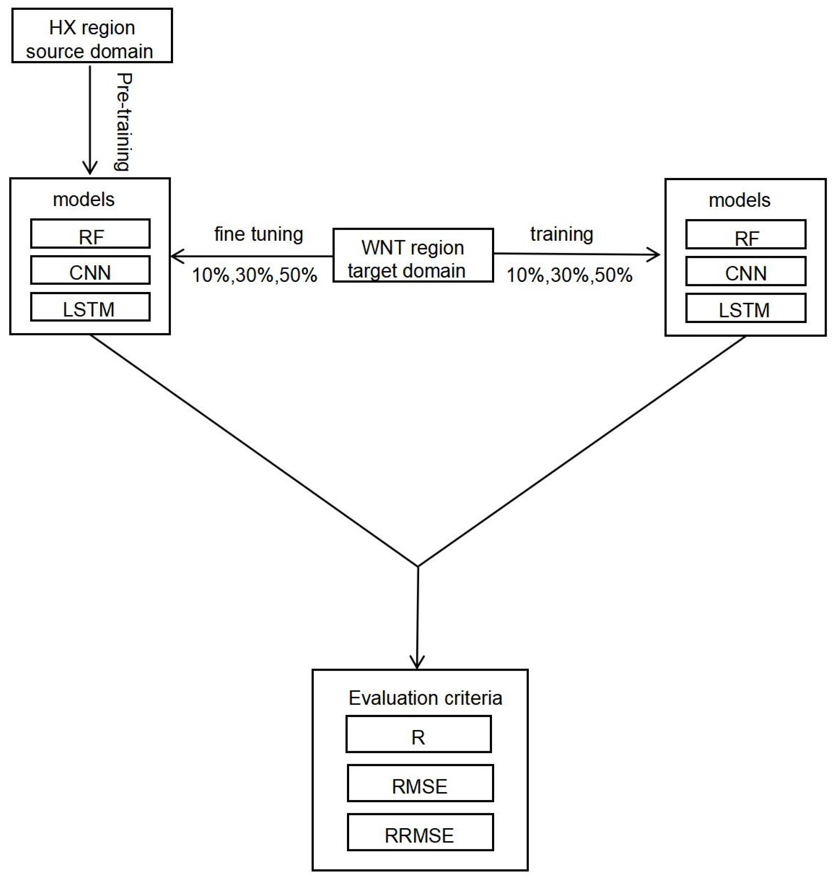
2.3.3. Transfer Learning Framework

As shown in Figure 2 in this study, the models (RF, CNN, and LSTM) are first built using the source domain data from HX region, which contains a larger number of training samples (173 SM sampling points) to construct the pre-trained models. Subsequently, a small number of samples from the target domain (WNT region) are used to fine-tune these pre-trained models. Specifically, this study fine-tunes the pre-trained models using 10%, 30%, and 50% of the target domain soil samples, while the remaining data are reserved for evaluating the performance of the fine-tuned models. By comparing the model performance under different fine-tuning ratios, the effect of the fine-tuning sample size on transfer performance is analyzed. The goal is to determine the optimal fine-tuning ratio under small sample conditions to evaluate the model’s transferability and generalization ability. The transfer learning method employed in this study leverages the pre-trained models, which have learned weights, to extract features for new tasks. The feature generation layers before the final fully connected layer are frozen [55].

2.3.4. Model Performance Evaluation

To evaluate the performance of the transfer learning framework and investigate the impact of different proportions of the target domain dataset used for fine-tuning on model performance, as well as the performance of different algorithms, this study compares four methods: (1) Source Domain Modeling: The RF, CNN, and LSTM algorithms are applied to model the source domain data. The potential of these algorithms for SM estimation is assessed, providing the foundation for subsequent transfer learning (

Table 3. Dataset details.

Dataset Name	Region	Total Samples	Each Soil Depth Layer Samples	Training Set Size/Testing Set Size	UAV Data
Source Domain (HX)	HX Region	519	173	7:3	Collected in the HX region.
Target Domain (WNT)	WNT Region	210	70	1:9 3:7 5:5	Collected in the WNT region.

). (2) Direct Transfer of the Source Domain Model: The trained source domain model is directly applied to the target domain for prediction. This serves as a control experiment with no transfer learning, allowing for comparison with the transfer learning models. (3) Fine-Tuning the Source Domain Model: The source domain model is fine-tuned using 10%, 30%, and 50% of the target domain samples, evaluating the effect of different fine-tuning data proportions on model performance to determine the optimal fine-tuning ratio. (4) Independent Training of the Target Domain Model: Using 10%, 30%, and 50% of the target domain samples, independent models are trained on the target domain, assessing whether transfer learning outperforms models trained solely on target domain data under limited sample conditions (Table 3). The flowchart is shown in Figure 3.

By comparing the four methods, the effectiveness of transfer learning under small sample conditions and its impact on improving model performance are analyzed. This also explores suitable fine-tuning strategies and algorithms to enhance the model’s generalization ability and cross-domain adaptability. To build the three different algorithm models, we perform multiple random training runs and take the average of the prediction results. This helps improve the accuracy and reliability of the model predictions. Multiple evaluation metrics, including the correlation coefficient (R), root mean square error (RMSE), and relative RMSE (RRMSE), are used to assess model performance. These metrics are widely applied in SM estimation [56]. A higher R value and smaller RMSE and RRMSE indicate better predictive capability of the model. The formulas for the model evaluation parameters are as follows:

$$\mathrm{R}={\displaystyle \frac{{\sum }_{\mathrm{i}=1}^{\mathrm{N}}\left[\left({\mathsf{\theta }}_{\mathrm{i}}^{\mathrm{E}}-{\mathsf{\theta }}_{\mathrm{Mean}}^{\mathrm{E}}\right)-\left({\mathsf{\theta }}_{\mathrm{i}}^{\mathrm{O}}-{\mathsf{\theta }}_{\mathrm{Mean}}^{\mathrm{O}}\right)\right]}{\sqrt{{\sum }_{\mathrm{i}=1}^{\mathrm{N}}{\left({\mathsf{\theta }}_{\mathrm{i}}^{\mathrm{E}}-{\mathsf{\theta }}_{\mathrm{Mean}}^{\mathrm{E}}\right)}^2}\sqrt{{\sum }_{\mathrm{i}=1}^{\mathrm{N}}{\left({\mathsf{\theta }}_{\mathrm{i}}^{\mathrm{O}}-{\mathsf{\theta }}_{\mathrm{Mean}}^{\mathrm{O}}\right)}^2}}}$$

(2)

$$RMSE=\sqrt{{\displaystyle \frac{1}{\mathrm{N}}}{\sum }_{\mathrm{i}=1}^{\mathrm{N}}{({\mathsf{\theta }}_{\mathrm{i}}^{\mathrm{E}}-{\mathsf{\theta }}_{\mathrm{i}}^{\mathrm{O}})}^2}$$

(3)

$$RRMSE={\displaystyle \frac{\mathrm{RMSE}}{{\mathsf{\theta }}_{\mathrm{Mean}}^{\mathrm{O}}}}\times 100$$

(4)

where $\mathrm{N}$ stands for the number of measured or estimated SM sample points and ${\mathsf{\theta }}^{\mathrm{O}}$ denotes the measured SM. Further more, ${\mathsf{\theta }}_{\mathrm{i}}^{\mathrm{E}}$ and ${\mathsf{\theta }}_{\mathrm{i}}^{\mathrm{O}}$ denote the i-th estimated SM and measured SM, respectively. ${\mathsf{\theta }}_{\mathrm{Mean} }^{\mathrm{E}}$ and ${\mathsf{\theta }}_{\mathrm{Mean}}^{\mathrm{O}}$ represent the mean values of estimated SM and measured SM, respectively.

3. Results

3.1. The Predictive Performance of the Source Domain Model

Figure 4 presents the modeling accuracy results using source domain (HX region) data at different depths (0–10 cm, 10–20 cm, 20–40 cm) with different algorithms (RF, CNN, LSTM). Overall, all three models exhibit significantly better performance in predicting shallow SM (0–10 cm) compared to deeper layers. The prediction accuracy for shallow soil is higher, indicating that the moisture characteristics of shallow soil are more distinct and easier for the models to capture. However, as soil depth increases, the complexity of SM characteristics also rises, leading to a decline in model performance. The performance of the three models varies at different depths.

LSTM shows outstanding performance in predicting shallow SM (0–10 cm), achieving an R value of 0.789, RMSE of 2.204%, and RRMSE of 7.432%. However, its performance significantly deteriorates with increasing soil depth. At the 10–20 cm depth, the R value drops to 0.472, and RRMSE increases to 15.132%. At the 20–40 cm depth, the R value further declines to 0.441, while RRMSE increases to 12.303%. CNN exhibits a similar trend in performance to LSTM. For example, at the 0–10 cm depth, it achieves high predictive accuracy with an R value of 0.765 and RMSE of 2.567%. At the 10–20 cm depth, the R value decreases to 0.455, and RMSE increases to 4.354%. At the 20–40 cm depth, CNN’s R value remains relatively stable at 0.454, suggesting that CNN’s prediction performance across different depths is relatively consistent. The RF model performs the best across all depths, demonstrating relatively consistent prediction accuracy at different soil depths, which indicates strong model robustness. This suggests that the RF model offers better stability and prediction advantages when training models with small sample data.

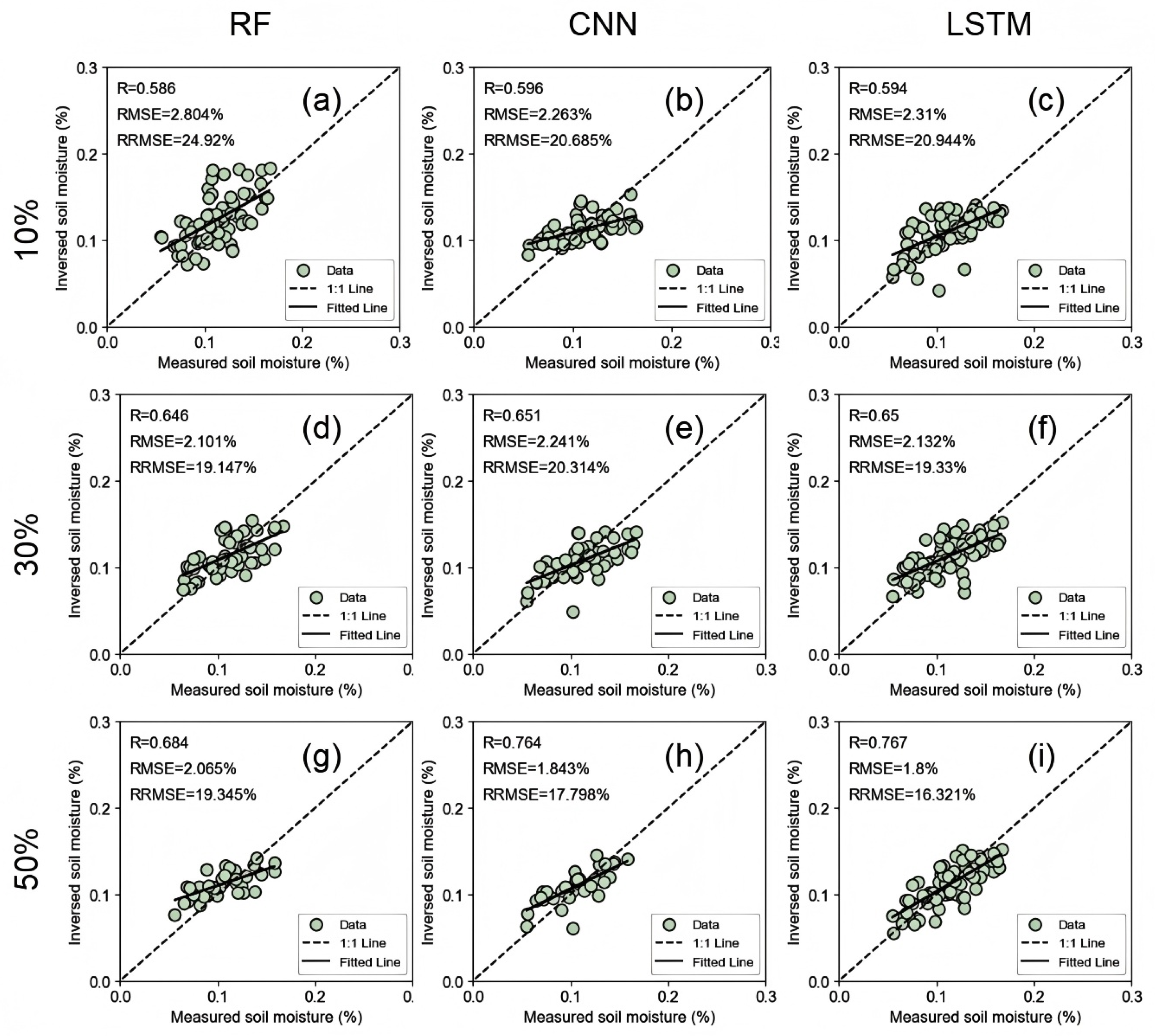
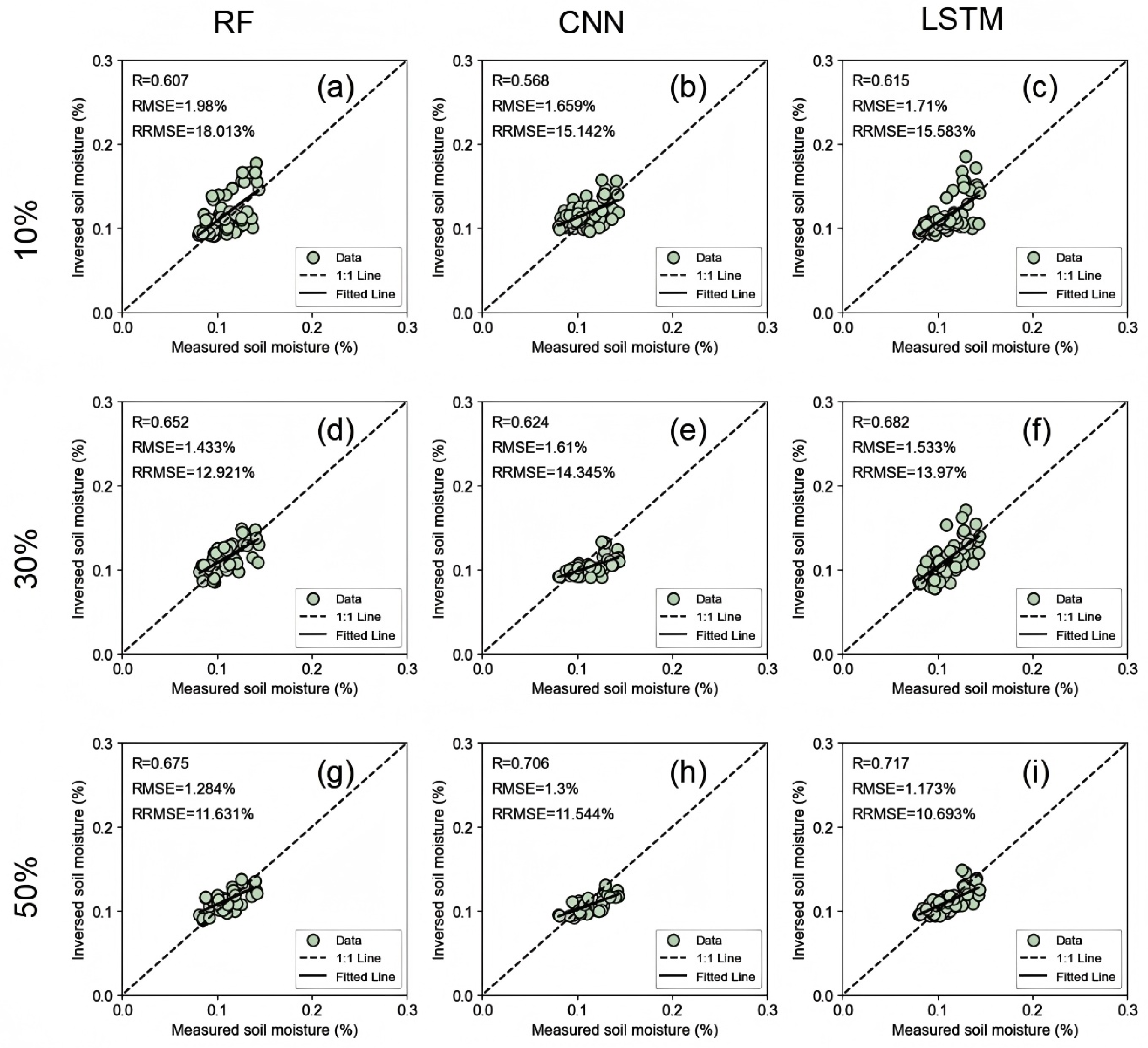
3.2. The Influence of Fine-Tuning Data with Different Proportions on the Performance of the Transfer Learning Framework

The results of fine-tuning the source domain model using different proportions of target domain data (10%, 30%, and 50%) are presented in Figure 5, Figure 6 and Figure 7. The findings indicate that increasing the proportion of training data is a crucial strategy for enhancing the model’s predictive accuracy. Specifically, the impact of data volume on model performance is particularly significant. Under the 10% fine-tuning condition, the RF, CNN, and LSTM models exhibit clear advantages, with rapid improvements in predictive performance to high levels. Notably, at the 30% fine-tuning data condition, all models show substantial performance enhancements across various depths, especially at 10 cm. For instance, at the 10 cm depth, the R values for the RF, CNN, and LSTM models increased by 10.24%, 9.23%, and 9.43%, respectively, while the RRMSE decreased by 23.17%, 1.79%, and 7.71%, respectively. These results suggest that all three models are highly sensitive to small sample fine-tuning data. Furthermore, the LSTM model demonstrates the most pronounced performance improvement at the 30% fine-tuning ratio, showing the fastest convergence compared to the other models.

As the data volume increases further, under the 50% fine-tuning condition, although the models continue to improve compared to the 30% fine-tuning condition, the disparities between the models become more evident. The RF model, even with 50% fine-tuning data, shows relatively minimal improvement, indicating that despite the increase in data volume, the performance enhancement remains constrained and significantly lower than that of the CNN and LSTM models. This suggests that the RF model has limitations in modeling complex data within the context of transfer learning. In contrast, the CNN model exhibits considerable improvement under the 50% fine-tuning condition, particularly at depths of 10 cm, 20 cm, and 40 cm, where the R values increased by 12.39%, 13.14%, and 11.68%, respectively. For the RF and LSTM models, the R values increased by 5.88%, 3.53%, 18.96%, 15.57%, 5.13%, and 10.53%, respectively.

At depths other than 0–10 cm, the CNN model demonstrates faster fine-tuning performance improvement compared to the LSTM model. However, the overall predictive accuracy of the CNN model remains lower than that of the LSTM model. The LSTM model shows significant improvement at a 30% fine-tuning ratio, with rapid convergence observed at 50%. In conclusion, LSTM demonstrated the greatest performance improvement and the best transferability. These results highlight the strong learning potential and adaptability of the LSTM model. In summary, the proportion of fine-tuning data directly influences the model’s ability to adapt to the target domain’s characteristics, particularly in deeper soil layers where data adequacy is critical for ensuring model performance.

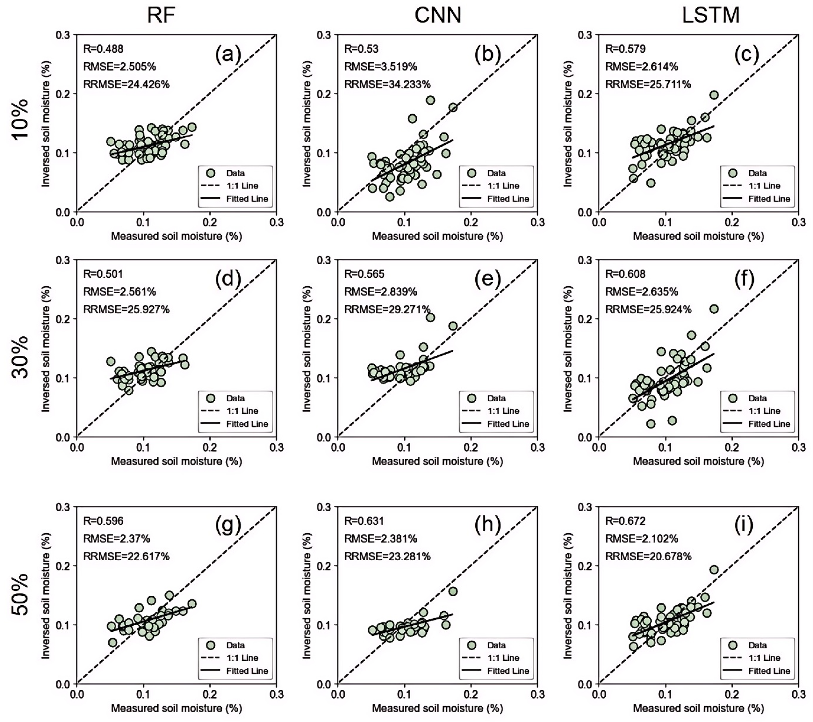
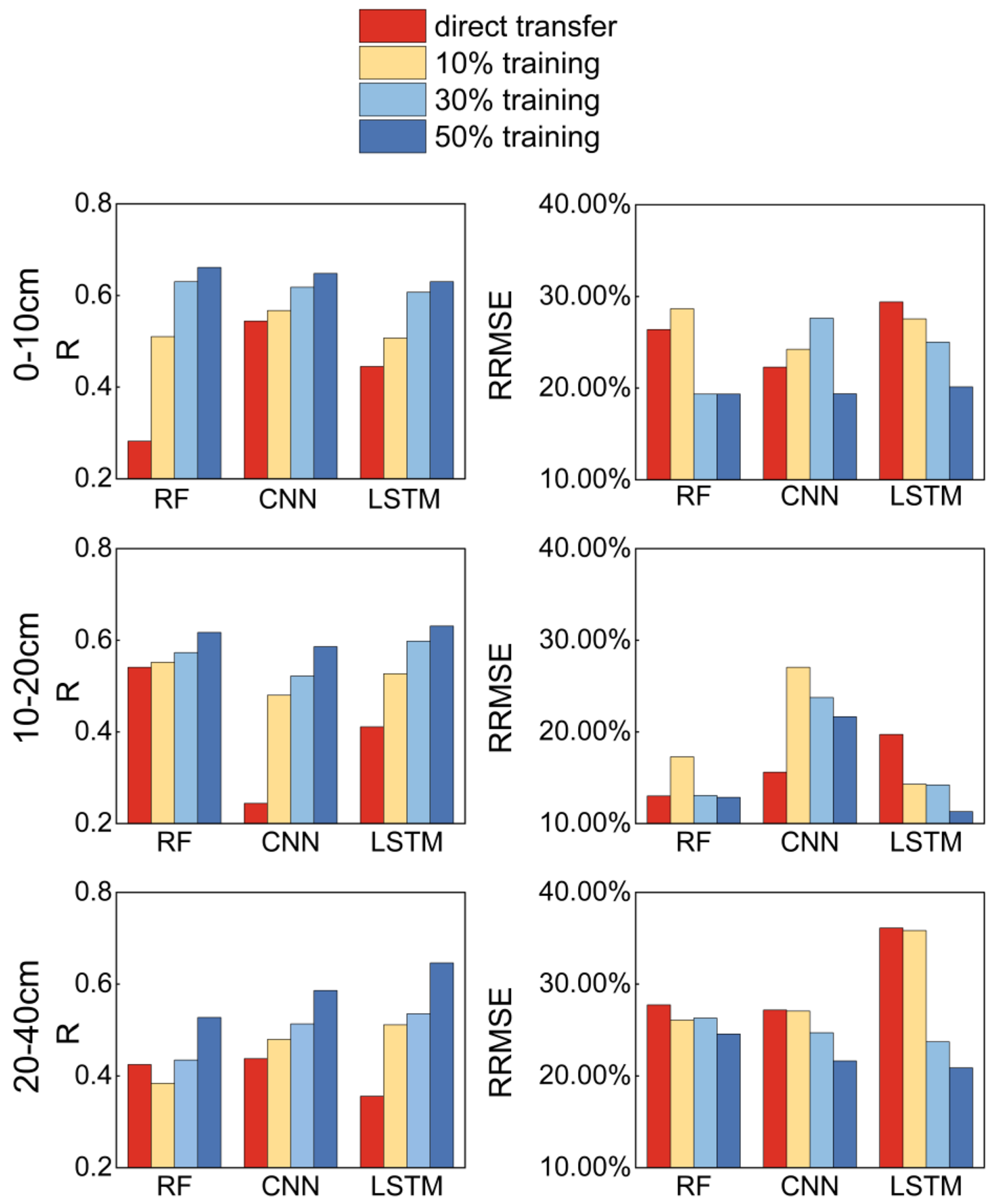
3.3. Comparison of Model Direct Transfer, Target Domain Training, and Transfer Learning Framework Performance

When the model is directly transferred from the source domain, the overall prediction accuracy is relatively low due to differences in data labels and environmental factors. As shown in Figure 8, at the 0–10 cm depth, the R-values for the three models (RF, CNN, and LSTM) are only 0.282, 0.544, and 0.445, respectively, which are far below the expected values. This result indicates that relying solely on source domain data for transfer prediction fails to adequately consider the characteristics of the target domain, leading to poor model adaptability.

When the models are independently trained using 10%, 30%, and 50% of the target domain data, their performance gradually improves with an increase in the training dataset proportion. Specifically, when only 10% of the target domain data are used for training, the overall accuracy of the three models remains low. Except for the RF model at the 0–10 cm depth and the CNN model at the 10–20 cm depth, the accuracy at other depths is similar to that observed under direct transfer, remaining well below the accuracy achieved through transfer learning with 10% fine-tuning data. This suggests that with limited target domain data, the models struggle to capture the target domain’s characteristics effectively, leading to slow improvements in accuracy.

As the proportion of the training dataset increases, especially when 30% of the target domain data are used, the performance of the models improves significantly. At the 0–10 cm depth, the R-values for the three models increase by 23.53%, 8.99%, and 19.72%, respectively, indicating that more target domain data help to enhance the model’s adaptability to the target domain. However, even with 30% target domain data, the accuracy remains lower than that achieved by the transfer learning framework with 30% fine-tuning, underscoring the importance of fine-tuning in improving model performance.

At the 10–20 cm and 20–40 cm depths, models trained with 30% of the target domain data perform similarly to the results obtained with 10% fine-tuning in the transfer learning framework. This suggests that as the dataset size increases, the models’ adaptability to these depths gradually improves. When 50% of the target domain data are used, the convergence speed slows, and the accuracy gains become more gradual, particularly in the 0–20 cm depth range. However, at the 20–40 cm depth, the model’s performance improvement is still notable. In this stage, models trained with 50% target domain data exhibit similar accuracy to the 30% fine-tuning results in the transfer learning framework, highlighting the significant performance enhancement that transfer learning provides under small sample conditions.

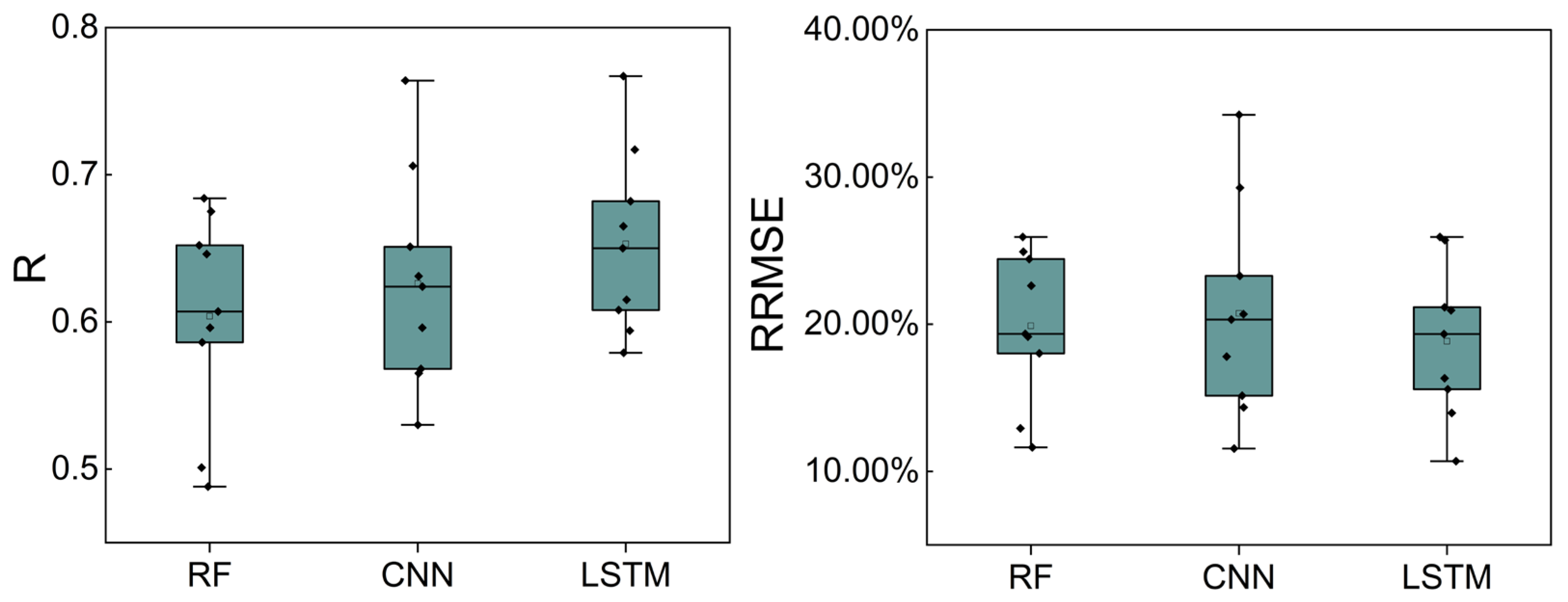
3.4. Overall Performance Comparison of RF, CNN, and LSTM Under the Framework of Transfer Learning

Figure 9 illustrates the overall performance comparison of the three models (RF, CNN, and LSTM) after transfer learning fine-tuning, with performance evaluated using two metrics: the correlation coefficient (R) and the normalized root mean square error (RRMSE). The results indicate that all three models exhibit a certain level of predictive capability, with CNN and LSTM generally outperforming RF. This is evidenced by higher medians and more concentrated distributions for CNN and LSTM. Specifically, the median R-values for CNN and LSTM are approximately 0.65, while RF’s median is slightly below 0.60. This suggests that deep learning models (CNN and LSTM) are better at capturing complex features of the data and can effectively extract multidimensional information to improve prediction accuracy.

However, there are notable differences in the stability of the models. CNN exhibits a wider distribution, with its prediction results fluctuating significantly across different experimental conditions, leading to higher variance and slightly lower stability compared to LSTM. In contrast, RF shows a narrower distribution but has a lower upper bound on prediction performance, reflecting its limitations in modeling complex nonlinear relationships.

The RRMSE values for all three models fall within the range of 0.10 to 0.30, indicating relatively low error levels. The median RRMSE for the LSTM model is the smallest, and its distribution is more concentrated, suggesting higher robustness and stability under different depth fine-tuning conditions. In contrast, CNN’s median RRMSE is close to that of LSTM, but its error distribution range is wider, particularly with higher extreme values, which may indicate issues such as overfitting or large prediction fluctuations. RF’s median RRMSE is notably higher than both CNN and LSTM, and its error range is also wider, further corroborating its limitations in modeling complex nonlinear data.

In summary, the analysis indicates that LSTM outperforms both CNN and RF in terms of performance and stability across both metrics (R and RRMSE), making it the optimal choice for fine-tuning under various depth conditions. Although CNN’s accuracy is comparable to LSTM’s, its broader fluctuation range suggests the need for further optimization of model hyperparameters or training strategies to enhance stability. RF, while suitable for simpler feature modeling tasks, falls short in both predictive capability and stability compared to deep learning models.

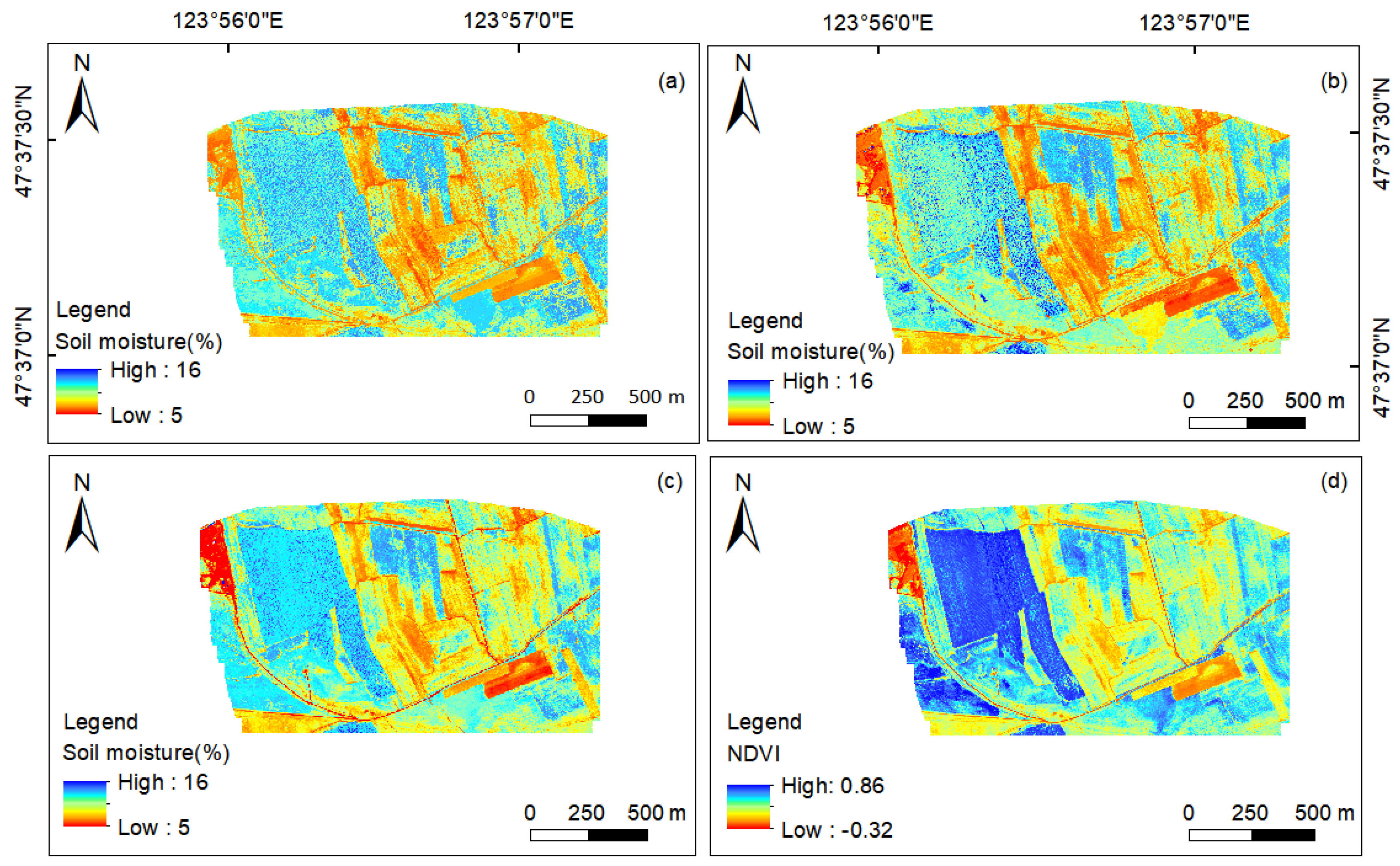
3.5. Analysis of Spatial Distribution of Study Area

Figure 10 illustrates the spatial distribution of soil moisture content. Figure 10a–c present the inversion results for RF, CNN, and LSTM algorithms, respectively, while Figure 10d displays the overall NDVI values across the study area. The inversion results from all three algorithms exhibit consistent spatial patterns, with soil moisture levels ranging between 5% and 16%. Each algorithm effectively captures the spatial distribution characteristics of soil moisture. Further analysis reveals a strong spatial correlation between higher NDVI values and increased soil moisture content, indicating a significant relationship between vegetation density and soil moisture.

Despite this consistency, notable differences exist in the detailed inversion results among the three algorithms, likely due to their distinct operational principles. Specifically, the RF and LSTM algorithms demonstrate more accurate and reasonable spatial distributions of soil moisture. According to the figure, the highest soil moisture content is observed in forested areas, followed by grasslands and farmlands, with bare soil areas exhibiting the lowest moisture levels.

4. Discussion

4.1. Comparison of Different Prediction Models and Limitations of Direct Transfer

In this study, we employed three models—RF, CNN, and LSTM—to estimate SM at different depths across two distinct study areas. Compared to CNN and LSTM models, the RF source domain model exhibited excellent predictive performance across varying depths and target domain models, highlighting the strong generalization ability of classical machine learning algorithms. This is due to RF’s lower computational requirements and simpler hyperparameter tuning process compared to deep learning models. Additionally, RF is robust to noise in the training data [57]. These findings align with the research by Cheng et al. [58]. However, despite RF’s high prediction accuracy in the source domain model, it demonstrated poor transferability [59], limiting its application in the target domain. To overcome the transfer limitations of RF, we introduced two deep learning models, CNN and LSTM. These models are considered among the most relevant deep learning techniques for hydrological prediction [60].

For shallow SM inversion (0–10 cm), both CNN and LSTM showed high prediction accuracy, with LSTM performing the best (R = 0.789, RRMSE = 7.432). However, for deeper soil layers (10–20 cm and 20–40 cm), RF outperformed CNN and LSTM in terms of predictive performance, maintaining stable model performance across different depths. This finding aligns with the research conducted by Teshome et al. [61], which suggests that deep learning models do not always outperform traditional machine learning algorithms in SM prediction.

When the source domain model is directly transferred to the target domain, the prediction accuracy significantly decreases [62], primarily due to distribution differences between the source and target domains. These differences may involve various factors such as feature space, climate conditions, and land use type changes. Such distribution discrepancies limit the model’s ability to generalize in the target domain, resulting in poor transferability [63].

Specifically, the differences in transfer performance among the three models can be attributed to the inherent characteristics of the algorithms as well as the distribution differences between the source and target domains: RF’s sensitivity to feature distribution changes restricts its generalization ability, leading to severely limited transferability. CNN and LSTM models perform poorly when feature extraction from the target domain is insufficient. Additionally, the small sample size and label distribution differences in the target domain exacerbate the limitations of transfer performance. For instance, Ma et al. [64] used a deep learning model trained on the source domain to predict maize yield in the target domain. Due to domain shift, the model’s performance deviated significantly from the target domain model. This highlights the need for more effective cross-domain alignment strategies in transfer learning tasks to better integrate the characteristics of both the source and target domains, ultimately improving model transferability.

4.2. The Advantages of Transfer Learning Frameworks in Few-Shot Transfer Learning

Fine-tuning is widely regarded as an efficient optimization strategy in transfer learning, where the source domain model is retrained with new data to improve its predictive performance in the target domain [65]. This method is particularly effective in small sample scenarios in the target domain, significantly enhancing model performance and enabling source domain models to exhibit greater adaptability across various domains [66]. Our study further validates the effectiveness of fine-tuning: By fine-tuning the source domain model with target domain data, the cross-regional soil moisture inversion accuracy of the model can be greatly improved. All fine-tuned source domain models outperformed models that were trained independently on target domain data from scratch, demonstrating the strong feature extraction and generalization capabilities of transfer learning in small-sample scenarios. For example, Zhu et al. [67] showed that after fine-tuning with only 10% of the target domain data, the model significantly improved its inversion accuracy in regions not covered by ground sample data, achieving an acceptable RMSE of 0.078 m³/m³ at other sites. Similarly, Yang et al. [68] confirmed that fine-tuning the source domain model in the target domain yielded superior performance compared to building a target domain model from scratch. Compared to traditional machine learning models (both source domain and target domain models), the proposed transfer learning framework significantly improves prediction accuracy. This is because traditional models require a large amount of data, and their performance often declines when applied to new regions with different data distributions, making generalization challenging. In contrast, the transfer learning framework effectively overcomes these limitations, enhancing adaptability across different regions while also alleviating the issue of data scarcity.

However, our study also revealed that the impact of different fine-tuning ratios on predictive accuracy varied significantly across different depths and models, adding complexity to the fine-tuning optimization process. Therefore, it is essential to determine the optimal fine-tuning ratio for each model at different depths to enhance the model’s adaptability and predictive capacity. In our study, for all three depths, the precision of the CNN and LSTM models when fine-tuned with 30% of the target domain data surpassed that of models fine-tuned with 50% of the target domain data. Moreover, when the fine-tuning ratio reached 50%, the models exhibited rapid convergence. This result confirms that deep learning models can still achieve good predictive performance with limited data and highlights the significant role of transfer learning in improving model performance [60].

4.3. Analysis of the Applicability of Different Algorithm Models in Transfer Learning

Different machine learning models exhibit significant variations in their performance during transfer learning, reflecting their suitability for SM prediction in transfer learning tasks. RF demonstrates certain advantages in capturing nonlinear relationships within the data, while maintaining good prediction accuracy and robustness. However, its limited adaptability in transfer learning restricts its generalization ability between source and target domains with large distribution differences [69]. In contrast, transfer deep learning models, such as CNN and LSTM, perform more effectively in this context [60]. For instance, Toth et al.’s research showed that after fine-tuning, the CNN model’s R² improved by approximately 100% in soil spectral prediction [70], demonstrating its strong transfer learning capability.

However, in this study, the fine-tuning ability of the CNN model was not as strong as that of the LSTM model. The LSTM model, in particular, exhibited remarkable performance in transfer learning, with substantial improvements in predictive accuracy after fine-tuning, especially when the target domain dataset was sufficiently large (e.g., 30% or 50%). This indicates that, with adequate data, the LSTM model’s nonlinear fitting capability outperforms others, showcasing stronger potential in transfer learning tasks. By combining transfer learning with deep learning, the model’s predictive ability in SM inversion was significantly enhanced, further expanding its application prospects in this domain. Future research could introduce additional transfer learning methods, such as domain alignment and feature transformation techniques, to further enhance the cross-domain adaptability of different models.

4.4. Future Research Directions

This study validates the effectiveness of fine-tuning strategies in transfer learning under small sample conditions and demonstrates their potential for soil moisture monitoring in agricultural watershed areas. However, several areas warrant further improvement. First, this study explores only fixed fine-tuning ratios (10%, 30%, 50%), whereas future research could develop dynamically adjustable fine-tuning strategies to optimize both fine-tuning proportions and target domain data scales. Second, the study focuses on two regions with similar climatic and geographic conditions. Expanding future research to a broader range of ecological environments would enhance the applicability and robustness of transfer learning. Finally, given the differences in transferability among various algorithms, future studies could explore hybrid models or ensemble learning approaches to improve model stability and predictive accuracy. These advancements would not only enhance the practicality of soil moisture monitoring but also facilitate the integration of UAV remote sensing with transfer learning techniques for more effective agricultural applications.

5. Conclusions

This study proposes a transfer learning-based framework for cross-regional SM inversion, leveraging RF, CNN, and LSTM models to address challenges posed by regional differences and the scarcity of target domain data. The study uses two typical small watersheds in Northeast China, HX and WNT, as case studies, systematically evaluating the impact of different algorithms, soil depths, and target domain training data proportions on SM prediction performance. It also explores the effects of fine-tuning using different proportions of target domain data. The results demonstrate that the fine-tuned models significantly outperform the direct application of the pre-trained source domain models. For instance, when only 10% of the target domain data are used, the fine-tuned model’s prediction accuracy closely approaches that of a model trained with 50% of the data. Transfer learning substantially enhances the prediction capability of models for the target domain, even when the available data are limited (10%), achieving reasonable prediction performance. As the training data increase (30% or 50%), deep learning models, especially LSTM, exhibit improved prediction accuracy. Additionally, this study reveals that the fine-tuning proportion significantly influences model performance. Higher fine-tuning proportions generally improve accuracy, but after a certain threshold (e.g., 50%), the performance gains plateau, and the model begins to converge rapidly.

The proposed transfer learning framework offers an effective solution for cross-regional UAV-based SM monitoring, significantly reducing the data requirements for the target domain while maintaining high prediction accuracy. This approach provides valuable insights for the widespread application of UAV-based SM monitoring, particularly in scenarios where data acquisition is challenging or regional differences are substantial, and it holds great potential for future applications.

References

1. Brocca, L.; Hasenauer, S.; Lacava, T.; Melone, F.; Moramarco, T.; Wagner, W.; Dorigo, W.; Matgen, P.; Martínez-Fernández, J.; Llorens, P. Soil moisture estimation through ASCAT and AMSR-E sensors: An intercomparison and validation study across Europe. Remote Sens. Environ. 2011, 115, 3390–3408. [Google Scholar] [CrossRef]
2. Peng, J.; Albergel, C.; Balenzano, A.; Brocca, L.; Cartus, O.; Cosh, M.H.; Crow, W.T.; Dabrowska-Zielinska, K.; Dadson, S.; Davidson, M.W.J.; et al. A roadmap for high-resolution satellite soil moisture applications—Confronting product characteristics with user requirements. Remote Sens. Environ. 2021, 252, 112162. [Google Scholar] [CrossRef]
3. Rahmani, A.; Golian, S.; Brocca, L. Multiyear monitoring of soil moisture over Iran through satellite and reanalysis soil moisture products. Int. J. Appl. Earth Obs. 2016, 48, 85–95. [Google Scholar] [CrossRef]
4. Luo, W.; Xu, X.; Liu, W.; Liu, M.; Li, Z.; Peng, T.; Xu, C.; Zhang, Y.; Zhang, R. UAV based soil moisture remote sensing in a karst mountainous catchment. Catena 2019, 174, 478–489. [Google Scholar] [CrossRef]
5. Robinson, D.A.; Campbell, C.S.; Hopmans, J.W.; Hornbuckle, B.K.; Jones, S.B.; Knight, R.; Ogden, F.; Selker, J.; Wendroth, O. Soil moisture measurement for ecological and hydrological watershed-scale observatories: A review. Vadose Zone J. 2008, 7, 358–389. [Google Scholar] [CrossRef]
6. Mukhlisin, M.; Astuti, H.W.; Wardihani, E.D.; Matlan, S.J. Techniques for ground-based soil moisture measurement: A detailed overview. Arab. J. Geosci. 2021, 14, 1–34. [Google Scholar] [CrossRef]
7. Guo, J.; Bai, Q.; Guo, W.; Bu, Z.; Zhang, W. Soil moisture content estimation in winter wheat planting area for multi-source sensing data using CNNR. Comput. Electron. Agr. 2022, 193, 106670. [Google Scholar] [CrossRef]
8. Zeng, L.; Hu, S.; Xiang, D.; Zhang, X.; Li, D.; Li, L.; Zhang, T. Multilayer soil moisture mapping at a regional scale from multisource data via a machine learning method. Remote Sens. 2019, 11, 284. [Google Scholar] [CrossRef]
9. Moore, I.D.; Grayson, R.B.; Ladson, A.R. Digital terrain modelling: A review of hydrological, geomorphological, and biological applications. Hydrol. Process. 1991, 5, 3–30. [Google Scholar] [CrossRef]
10. Chen, H.; Zhang, W.; Wang, K.; Fu, W. Soil moisture dynamics under different land uses on karst hillslope in northwest Guangxi, China. Environ. Earth Sci. 2010, 61, 1105–1111. [Google Scholar] [CrossRef]
11. Ma, K.M.; Fu, B.J.; Liu, S.L.; Guan, W.B.; Liu, G.H.; Lü, Y.H.; Anand, M. Multiple-scale soil moisture distribution and its implications for ecosystem restoration in an arid river valley, China. Land Degrad. Dev. 2004, 15, 75–85. [Google Scholar] [CrossRef]
12. Peng, J.; Tanguy, M.; Robinson, E.L.; Pinnington, E.; Evans, J.; Ellis, R.; Cooper, E.; Hannaford, J.; Blyth, E.; Dadson, S. Estimation and evaluation of high-resolution soil moisture from merged model and Earth observation data in the Great Britain. Remote Sens. Environ. 2021, 264, 112610. [Google Scholar] [CrossRef]
13. Hill, D.J.; Tarasoff, C.; Whitworth, G.E.; Baron, J.; Bradshaw, J.L.; Church, J.S. Utility of unmanned aerial vehicles for mapping invasive plant species: A case study on yellow flag iris (Iris pseudacorus L.). Int. J. Remote. Sens. 2017, 38, 2083–2105. [Google Scholar] [CrossRef]
14. Cheng, M.; Li, B.; Jiao, X.; Huang, X.; Fan, H.; Lin, R.; Liu, K. Using multimodal remote sensing data to estimate regional-scale soil moisture content: A case study of Beijing, China. Agr. Water Manag. 2022, 260, 107298. [Google Scholar] [CrossRef]
15. Seo, M.; Shin, H.; Tsourdos, A. Soil moisture retrieval model design with multispectral and infrared images from unmanned aerial vehicles using convolutional neural network. Agronomy 2021, 11, 398. [Google Scholar] [CrossRef]
16. Holloway, J.; Mengersen, K. Statistical Machine Learning Methods and Remote Sensing for Sustainable Development Goals: A Review. Remote Sens. 2018, 10, 1365. [Google Scholar] [CrossRef]
17. Maimaitijiang, M.; Sagan, V.; Sidike, P.; Hartling, S.; Esposito, F.; Fritschi, F.B. Soybean yield prediction from UAV using multimodal data fusion and deep learning. Remote Sens. Environ. 2020, 237, 111599. [Google Scholar] [CrossRef]
18. Chen, Z.; Chen, H.; Dai, Q.; Wang, Y.; Hu, X. Estimation of Soil Moisture during Different Growth Stages of Summer Maize under Various Water Conditions Using UAV Multispectral Data and Machine Learning. Agronomy 2024, 14, 2008. [Google Scholar] [CrossRef]
19. Zhang, Y.; Han, W.; Zhang, H.; Niu, X.; Shao, G. Evaluating soil moisture content under maize coverage using UAV multimodal data by machine learning algorithms. J. Hydrol. 2023, 617, 129086. [Google Scholar] [CrossRef]
20. Zhu, X.X.; Tuia, D.; Mou, L.; Xia, G.; Zhang, L.; Xu, F.; Fraundorfer, F. Deep learning in remote sensing: A comprehensive review and list of resources. IEEE Geosci. Remote Sens. Mag. 2017, 5, 8–36. [Google Scholar] [CrossRef]
21. Hegazi, E.H.; Yang, L.; Huang, J. A convolutional neural network algorithm for soil moisture prediction from Sentinel-1 SAR images. Remote Sens. 2021, 13, 4964. [Google Scholar] [CrossRef]
22. Ahmed, A.M.; Deo, R.C.; Ghahramani, A.; Raj, N.; Feng, Q.; Yin, Z.; Yang, L. LSTM integrated with Boruta-random forest optimiser for soil moisture estimation under RCP4. 5 and RCP8. 5 global warming scenarios. Stoch. Environ. Res. Risk Assess. 2021, 35, 1851–1881. [Google Scholar] [CrossRef]
23. Fu, B.; Wang, J.; Chen, L.; Qiu, Y. The effects of land use on soil moisture variation in the Danangou catchment of the Loess Plateau, China. Catena 2003, 54, 197–213. [Google Scholar] [CrossRef]
24. Xu, G.; Huang, M.; Li, P.; Li, Z.; Wang, Y. Effects of land use on spatial and temporal distribution of soil moisture within profiles. Environ. Earth Sci. 2021, 80, 128. [Google Scholar] [CrossRef]
25. Bulut, B.; Yilmaz, M.T.; Afshar, M.H.; Şorman, A.Ü.; Yücel, İ.; Cosh, M.H.; Şimşek, O. Evaluation of remotely-sensed and model-based soil moisture products according to different soil type, vegetation cover and climate regime using station-based observations over Turkey. Remote Sens. 2019, 11, 1875. [Google Scholar] [CrossRef]
26. Koster, R.D.; Guo, Z.; Yang, R.; Dirmeyer, P.A.; Mitchell, K.; Puma, M.J. On the nature of soil moisture in land surface models. J. Clim. 2009, 22, 4322–4335. [Google Scholar] [CrossRef]
27. Kornelsen, K.C.; Coulibaly, P. Root-zone soil moisture estimation using data-driven methods. Water Resour. Res. 2014, 50, 2946–2962. [Google Scholar] [CrossRef]
28. Dekker, A.G.; Peters, S.; Vos, R.; Rijkeboer, M. Remote sensing for inland water quality detection and monitoring: State-of-the-art application in Friesland waters. In GIS and Remote Sensing Techniques in Land-and Water-Management; Springer: Dordrecht, The Netherlands, 2001; pp. 17–38. [Google Scholar]
29. Wikle, C.K. A kernel-based spectral model for non-Gaussian spatio-temporal processes. Stat. Model. 2002, 2, 299–314. [Google Scholar] [CrossRef]
30. Pan, S.J.; Yang, Q. A survey on transfer learning. IEEE Trans. Knowl. Data Eng. 2009, 22, 1345–1359. [Google Scholar] [CrossRef]
31. Weiss, K.; Khoshgoftaar, T.M.; Wang, D. A survey of transfer learning. J. Big Data 2016, 3, 9. [Google Scholar] [CrossRef]
32. Pires De Lima, R.; Marfurt, K. Convolutional neural network for remote-sensing scene classification: Transfer learning analysis. Remote Sens. 2019, 12, 86. [Google Scholar] [CrossRef]
33. Li, J.; Xiao, Z.; Sun, R.; Song, J. Retrieval of the leaf area index from visible infrared imaging radiometer suite (VIIRS) surface reflectance based on unsupervised domain adaptation. Remote Sens. 2022, 14, 1826. [Google Scholar] [CrossRef]
34. Liu, L.; Ji, M.; Buchroithner, M. Transfer learning for soil spectroscopy based on convolutional neural networks and its application in soil clay content mapping using hyperspectral imagery. Sensors 2018, 18, 3169. [Google Scholar] [CrossRef] [PubMed]
35. Wang, A.X.; Tran, C.; Desai, N.; Lobell, D.; Ermon, S. in Deep transfer learning for crop yield prediction with remote sensing data. In Proceedings of the 1st ACM SIGCAS Conference on Computing and Sustainable Societies, Menlo Park, CA, USA, 20–22 June 2018; Association for Computing Machiner: New York, NY, USA, 2018; pp. 1–5. [Google Scholar]
36. Pu, F.; Ding, C.; Chao, Z.; Yu, Y.; Xu, X. Water-quality classification of inland lakes using landsat8 images by convolutional neural networks. Remote Sens. 2019, 11, 1674. [Google Scholar] [CrossRef]
37. FAO (Food and Agriculture Organization of the United Nations). World Reference Base for Soil Resources 2014. In International Soil Classification System for Naming Soils and Creating Legends for Soil Maps; World Soil Res ources Reports 106; FAO: Rome, Italy, 2015. [Google Scholar]
38. Liu, B.; Wen, Y.; Lin, L.; Wen, X.; Gao, R.; Zhang, B.; Li, T.; Yao, S. Variations in soil quality indicators under different cultivation ages and slope positions of arable land in the Mollisol region of China. Catena 2024, 246, 108418. [Google Scholar] [CrossRef]
39. Wen, Y.; Liu, B.; Lin, L.; Hu, M.; Wen, X.; Li, T.; Rong, J.; Yao, S. Shelterbelt effects on soil redistribution on an arable slope by wind and water. Catena 2024, 241, 108044. [Google Scholar] [CrossRef]
40. Huete, A.R. A soil-adjusted vegetation index (SAVI). Remote Sens. Environ. 1988, 25, 295–309. [Google Scholar] [CrossRef]
41. Mishra, S.; Mishra, D.R. Normalized difference chlorophyll index: A novel model for remote estimation of chlorophyll-a concentration in turbid productive waters. Remote Sens. Environ. 2012, 117, 394–406. [Google Scholar]
42. Rondeaux, G.; Steven, M.; Baret, F. Optimization of soil-adjusted vegetation indices. Remote Sens. Environ. 1996, 55, 95–107. [Google Scholar]
43. Rouse, J.W.; Haas, R.H.; Schell, J.A.; Deering, D.W. Monitoring vegetation systems in the Great Plains with ERTS. NASA Spec. Publ. 1974, 351, 309. [Google Scholar]
44. Wang, F.; Huang, J.; Tang, Y.; Wang, X. New vegetation index and its application in estimating leaf area index of rice. Rice Sci. 2007, 14, 195–203. [Google Scholar]
45. Zarco-Tejada, P.J.; Berjón, A.; Lopez-Lozano, R.; Miller, J.R.; Martín, P.; Cachorro, V.; González, M.R.; De Frutos, A. Assessing vineyard condition with hyperspectral indices: Leaf and canopy reflectance simulation in a row-structured discontinuous canopy. Remote Sens. Environ. 2005, 99, 271–287. [Google Scholar] [CrossRef]
46. Huete, A.; Didan, K.; Miura, T.; Rodriguez, E.P.; Gao, X.; Ferreira, L.G. Overview of the radiometric and biophysical performance of the MODIS vegetation indices. Remote Sens. Environ. 2002, 83, 195–213. [Google Scholar] [CrossRef]
47. Mathieu, R.; Pouget, M.; Cervelle, B.; Escadafal, R. Relationships between satellite-based radiometric indices simulated using laboratory reflectance data and typic soil color of an arid environment. Remote Sens. Environ. 1998, 66, 17–28. [Google Scholar]
48. Escadafal, R. Remote sensing of arid soil surface color with Landsat thematic mapper. Adv. Space Res. 1989, 9, 159–163. [Google Scholar]
49. Haboudane, D.; Miller, J.R.; Tremblay, N.; Zarco-Tejada, P.J.; Dextraze, L. Integrated narrow-band vegetation indices for prediction of crop chlorophyll content for application to precision agriculture. Remote Sens. Environ. 2002, 81, 416–426. [Google Scholar]
50. Svetnik, V.; Liaw, A.; Tong, C.; Culberson, J.C.; Sheridan, R.P.; Feuston, B.P. Random forest: A classification and regression tool for compound classification and QSAR modeling. J. Chem. Inf. Comput. Sci. 2003, 43, 1947–1958. [Google Scholar] [CrossRef]
51. LeCun, Y.; Boser, B.; Denker, J.; Henderson, D.; Howard, R.; Hubbard, W.; Jackel, L. Handwritten digit recognition with a back-propagation network. Adv. Neural Inf. Process. Syst. 1989, 2. [Google Scholar]
52. Wang, N.; Chen, F.; Yu, B.; Qin, Y. Segmentation of large-scale remotely sensed images on a Spark platform: A strategy for handling massive image tiles with the MapReduce model. ISPRS J. Photogramm. 2020, 162, 137–147. [Google Scholar] [CrossRef]
53. Hochreiter, S. Long Short-term Memory. Neural Comput. 1997, 9, 1735–1780. [Google Scholar]
54. Fang, K.; Shen, C. Near-real-time forecast of satellite-based soil moisture using long short-term memory with an adaptive data integration kernel. J. Hydrometeorol. 2020, 21, 399–413. [Google Scholar]
55. Ghazi, M.M.; Yanikoglu, B.; Aptoula, E. Plant identification using deep neural networks via optimization of transfer learning parameters. Neurocomputing 2017, 235, 228–235. [Google Scholar]
56. Li, S.; Han, Y.; Li, C.; Wang, J. A novel framework for multi-layer soil moisture estimation with high spatio-temporal resolution based on data fusion and automated machine learning. Agr. Water Manag. 2024, 306, 109173. [Google Scholar]
57. Belgiu, M.; Drăguţ, L. Random forest in remote sensing: A review of applications and future directions. ISPRS J. Photogramm. 2016, 114, 24–31. [Google Scholar]
58. Cheng, M.; Jiao, X.; Liu, Y.; Shao, M.; Yu, X.; Bai, Y.; Wang, Z.; Wang, S.; Tuohuti, N.; Liu, S. Estimation of soil moisture content under high maize canopy coverage from UAV multimodal data and machine learning. Agr. Water Manag. 2022, 264, 107530. [Google Scholar]
59. Skobalski, J.; Sagan, V.; Alifu, H.; Al Akkad, O.; Lopes, F.A.; Grignola, F. Bridging the gap between crop breeding and GeoAI: Soybean yield prediction from multispectral UAV images with transfer learning. ISPRS J. Photogramm. 2024, 210, 260–281. [Google Scholar]
60. Li, Q.; Wang, Z.; Shangguan, W.; Li, L.; Yao, Y.; Yu, F. Improved daily SMAP satellite soil moisture prediction over China using deep learning model with transfer learning. J. Hydrol. 2021, 600, 126698. [Google Scholar]
61. Teshome, F.T.; Bayabil, H.K.; Schaffer, B.; Ampatzidis, Y.; Hoogenboom, G. Improving soil moisture prediction with deep learning and machine learning models. Comput. Electron. Agr. 2024, 226, 109414. [Google Scholar] [CrossRef]
62. Ma, Y.; Chen, S.; Ermon, S.; Lobell, D.B. Transfer learning in environmental remote sensing. Remote Sens. Environ. 2024, 301, 113924. [Google Scholar] [CrossRef]
63. Michau, G.; Fink, O. Unsupervised transfer learning for anomaly detection: Application to complementary operating condition transfer. Knowl.-Based Syst. 2021, 216, 106816. [Google Scholar]
64. Ma, Y.; Zhang, Z.; Yang, H.L.; Yang, Z. An adaptive adversarial domain adaptation approach for corn yield prediction. Comput. Electron. Agr. 2021, 187, 106314. [Google Scholar] [CrossRef]
65. Gao, Y.; Ruan, Y.; Fang, C.; Yin, S. Deep learning and transfer learning models of energy consumption forecasting for a building with poor information data. Energ. Build. 2020, 223, 110156. [Google Scholar] [CrossRef]
66. Simonyan, K. Very deep convolutional networks for large-scale image recognition. arXiv 2014, arXiv:1409.1556. [Google Scholar]
67. Zhu, L.; Dai, J.; Liu, Y.; Yuan, S.; Qin, T.; Walker, J.P. A cross-resolution transfer learning approach for soil moisture retrieval from Sentinel-1 using limited training samples. Remote Sens. Environ. 2024, 301, 113944. [Google Scholar] [CrossRef]
68. Yang, J.; Yang, Q.; Hu, F.; Shao, J.; Wang, G. A climate-adaptive transfer learning framework for improving soil moisture estimation in the Qinghai-Tibet Plateau. J. Hydrol. 2024, 630, 130717. [Google Scholar] [CrossRef]
69. Sudhakara, B.; Bhattacharjee, S. Prediction of High-Resolution Soil Moisture Using Multi-source Data and Machine Learning. In International Conference on Distributed Computing and Intelligent Technology; Springer: Cham, Switzerland, 2024; pp. 282–292. [Google Scholar]
70. Tóth, G.; Jones, A.; Montanarella, L. The LUCAS topsoil database and derived information on the regional variability of cropland topsoil properties in the European Union. Environ. Monit. Assess. 2013, 185, 7409–7425. [Google Scholar] [CrossRef]
Figure 1. (a) Location of the study regions, Hongxing (HX) and Woniutu (WNT), within the Mollisol region of Northeast China. (b) Specific sampling point test settings for the Hongxing (HX) region. (c) Specific sampling point test settings for the Woniutu (WNT) region.
Agronomy 15 00759 g001
Figure 2. Transfer learning frameworks based on Random Forest (RF), Convolutional Neural Network (CNN), and Long Short-Term Memory (LSTM).
Agronomy 15 00759 g002
Figure 3. The specific flowchart of data analysis and processing using different indices and algorithm models.
Agronomy 15 00759 g003
Figure 4. The modeling outcomes for the source domain (HX area) using three model approaches: Random Forest (RF), Convolutional Neural Network (CNN), and Long Short-Term Memory (LSTM), across three depth intervals: 0–10 cm, 10–20 cm, and 20–40 cm. Among them, (ac) are the inversion results of the RF, CNN, and LSTM models in the 0–10 cm range, (df) are the inversion results in the 10–20 cm range, and (gi) are the inversion results in the 20–40 cm range.
Agronomy 15 00759 g004
Figure 5. The accuracy outcomes of the three source domain models—Random Forest (RF), Convolutional Neural Network (CNN), and Long Short-Term Memory (LSTM)—after fine-tuning with target domain data proportions of 10%, 30%, and 50% at a depth of 0–10 cm. Among them, (ac) are the inversion results after fine-tuning the RF, CNN, and LSTM models with 10% of the target domain data, (df) are the inversion results after fine-tuning with 30% of the target domain data, and (gi) are the inversion results after fine-tuning with 50% of the target domain data.
Agronomy 15 00759 g005
Figure 6. The accuracy outcomes of the three source domain models—Random Forest (RF), Convolutional Neural Network (CNN), and Long Short-Term Memory (LSTM)—after fine-tuning with target domain data proportions of 10%, 30%, and 50% at a depth of 10–20 cm. Among them, (ac) are the inversion results after fine-tuning the RF, CNN, and LSTM models with 10% of the target domain data, (df) are the inversion results after fine-tuning with 30% of the target domain data, and (gi) are the inversion results after fine-tuning with 50% of the target domain data.
Agronomy 15 00759 g006
Figure 7. The accuracy outcomes of the three source domain models—Random Forest (RF), Convolutional Neural Network (CNN), and Long Short-Term Memory (LSTM)—after fine-tuning with target domain data proportions of 10%, 30%, and 50% at a depth of 20–40 cm. Among them, (ac) are the inversion results after fine-tuning the RF, CNN, and LSTM models with 10% of the target domain data, (df) are the inversion results after fine-tuning with 30% of the target domain data, and (gi) are the inversion results after fine-tuning with 50% of the target domain data.
Agronomy 15 00759 g007
Figure 8. A comparison of the modeling accuracy between direct transfer of the source domain model and fine-tuning with different proportions of target domain data (10%, 30%, and 50%) across various depth layers (0–10 cm, 10–20 cm, and 20–40 cm).
Agronomy 15 00759 g008
Figure 9. The overall accuracy of the three models—Random Forest (RF), Convolutional Neural Network (CNN), and Long Short-Term Memory (LSTM) is evaluated.
Agronomy 15 00759 g009
Figure 10. The spatial distribution maps of SM in the 0–10 cm soil layer generated by the proposed transfer learning model framework are presented. (a) The spatial distribution map of SMC generated by the Random Forest (RF) model; (b) the spatiotemporal distribution map generated by the Convolutional Neural Network (CNN) model; and (c) the spatiotemporal distribution map generated by the Long Short-Term Memory (LSTM) network. (d) The NDVI values of the study area.
Agronomy 15 00759 g010