Predicting Minimum Temperatures of Plastic Greenhouse During Strawberry Growing in Changfeng, China: A Comparison of Machine Learning Algorithms and Multiple Linear Regression

Abstract

Scientific management and environmental regulation of facility strawberries depends on the level of accurate prediction and forecasting of low temperature freezes in plastic greenhouses during winter and spring strawberry cultivation. Accurate identification of potential factors affecting layer-by-layer minimum temperatures in plastic greenhouses and selection of optimal forecasting methods are important for safe strawberry production. However, the identification of important drivers of minimum temperatures in plastic greenhouses and the prediction of potential drivers of use are still unclear. In this study, we used Classification and Regression Tree (CART) to identify the importance of the potential factors affecting the minimum temperatures at different depths and different heights of plastic greenhouses. Random forest (RF), back-propagation (BP), and multiple linear regression (MLR) were used to establish the minimum temperature prediction models for plastic greenhouses at different depths and heights, respectively. The results showed that T_smin10, T_smin25, T_amin150, T_amin320, and T_amin150 were the most important variables explaining the changes in minimum temperatures at heights T_smin25, T_smin10, T_smin2, T_amin150, and T_amin320 respectively. RF, BP performed much better than MLR, as it showed much lower error indices (AE and RMSE) and higher R² than MLR. The superiority of RF and BP in predicting minimum temperatures is related to their ability to deal with non-linear and hierarchical relationships between minimum temperatures and predictors. The low-temperature frost protection and fine management of strawberries in the Changfeng area can be related to the prediction method of minimum temperature in plastic greenhouses constructed in this study.

1. Introduction

The strawberry (Fragaria × ananassa Duch.) is a perennial herbaceous plant belonging to the berry fruit family (Rosaceae), originating from South America. Strawberry berries are bright red in colour, aromatic and juicy, sweet and sour, nutritious, and rich in vitamins, polyphenols, and other antioxidants, with high nutritional and economic value, and are loved by consumers [1,2]. In recent years, facility cultivation has been the main cultivation of strawberries, and Changfeng County is the first major county for strawberry production in China. At present, the strawberry planting area has reached 140,000 hm², with an annual output of over 360,000 t and a strawberry brand value of 10.2 billion yuan in Changfeng County. Strawberry is a light-loving, warm and cool climate plant. In different stages of development, it has different temperature requirements, with an optimum temperature of 15–25 °C; too high or too low a temperature will affect the growth and development of strawberry and yield formation [3,4]. Winter and spring is the critical period of facility strawberry production, when the strawberry is in a flowering and fruiting period, a wide range of cold wave cooling weather will cause the internal temperature of plastic greenhouses to drop, and ultimately lead to a large area of strawberry yield reduction, or even total loss. Therefore, it is of great practical significance to strengthen the monitoring and forecasting of minimum temperature at different depths and height layers in plastic greenhouses in winter and spring for strawberry disaster prevention and mitigation, and for improving quality and efficiency.

It has been shown that the microclimate in the plastic greenhouses and the external meteorological conditions have a certain correlation, as well as the existence of certain differences and hysteresis, existing obvious phenomenon of “shed temperature inversion” [5,6,7]. Daily management of plastic greenhouses and weather conditions often have a great influence on internal meteorological conditions, making the microclimate prediction in greenhouses very difficult [8,9]. Domestic and foreign research on numerical simulation of greenhouses temperature began in the 1960s, with research methods focusing on two categories: physical models and statistical models [10,11,12]. According to the theory of physical model combined with advanced fluid mechanics technology, the former simulated and predicted the internal environment under natural ventilation of single-span pitched roof greenhouses, which achieved better simulation results and provided a scientific basis for the structural optimisation and production management of solar greenhouses [13,14,15]. Statistical models mostly focus on simulating and predicting the elements in the greenhouses based on the differences in meteorological conditions inside and outside the greenhouses, and then screening out the key meteorological elements that affect the temperature changes in the greenhouse. The most representative statistical models are autoregressive models, multi-objective evolutionary algorithms, principal component analysis, harmonic methods, BP neural networks, support vector machines, etc. [8,16,17,18,19,20]. Physical models have strong predictive rationality and good interpretability, but the models require more parameters, complex methods, and larger computational errors. Statistical models are widely used in greenhouse microclimate characterisation because of their computational simplicity.

In the era of big data, the advantages of using machine learning to handle non-linear and hierarchical problems and solve high-dimensional variables [21,22,23] have been successfully applied in predicting the onset of winter wheat flowering [24], predicting pear flowering [25], predicting the ear rate of ruderalis disease [26], and predicting wheat yield [27]. However, little research has been reported on layer-by-layer minimum temperature prediction in plastic greenhouses using machine learning techniques. Given the rapid dynamics of minimum temperatures in plastic greenhouses, accurate prediction of minimum temperatures in plastic greenhouses is critical for safe strawberry production.

The objectives of this study were as follows: (1) To accurately identify the main meteorological factors affecting minimum temperatures at different soil depths and at different heights in plastic greenhouses using the CART method. (2) To predict minimum temperatures at different soil depths and at different heights in plastic greenhouses using the RF, BP, and MLR models, and to compare the performance of the three models.

2. Materials and Methods

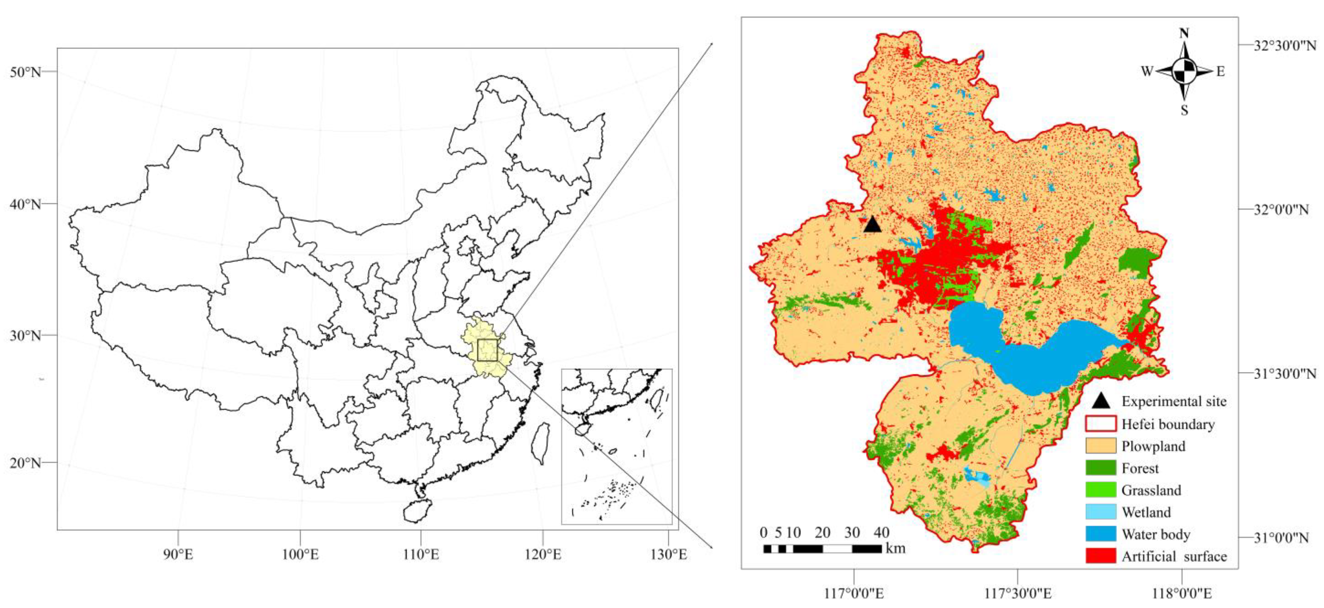
2.1. Study Area

The experiment was conducted at the Hefei Agrometeorological Experimental Station in central Anhui Province, China (117°03′ E, 31°57′ N) (Figure 1). The experimental area covers about 113.7 ha, with an elevation of 49.8 m above sea level. The experiment has a subtropical monsoon climate, with a mean annual temperature, rainfall, and daylight hours of 16.2 °C, 1000.9 mm, and 1868.1 h, respectively. The soil of the experimental site was loamy clay, acidic, and of medium fertility. Extreme cold events occur in this region from November to the following March, with the critical development period for facilities strawberry (flowering and fruiting period). The plastic greenhouses for growing strawberries are single span, arched roof greenhouses covering an area of 2 hectares, divided north and south, with a 2-layer trellis structure, with an additional layer of black mulch applied during planting. The outer greenhouse is 86.9 m long and 3.3 m high, and the inner greenhouse is 85.6 m long and 3 m high, made of 0.1 mm thick polyethylene film with over 90% light transmission. The strawberry variety for testing is ‘Red Face’. The strawberries are planted in plastic greenhouses at the beginning of September and harvested in May of the following year. The strawberries were grown in plastic greenhouses with a total of 7 rows, each 16.7 m long and 1.5 m wide, with a drainage ditch 40 cm wide and deep between the rows, and 1 plant per hole. Strawberry growing in plastic greenhouses was carried out in the usual local way, with additional daily ventilation management and without any heating measures.

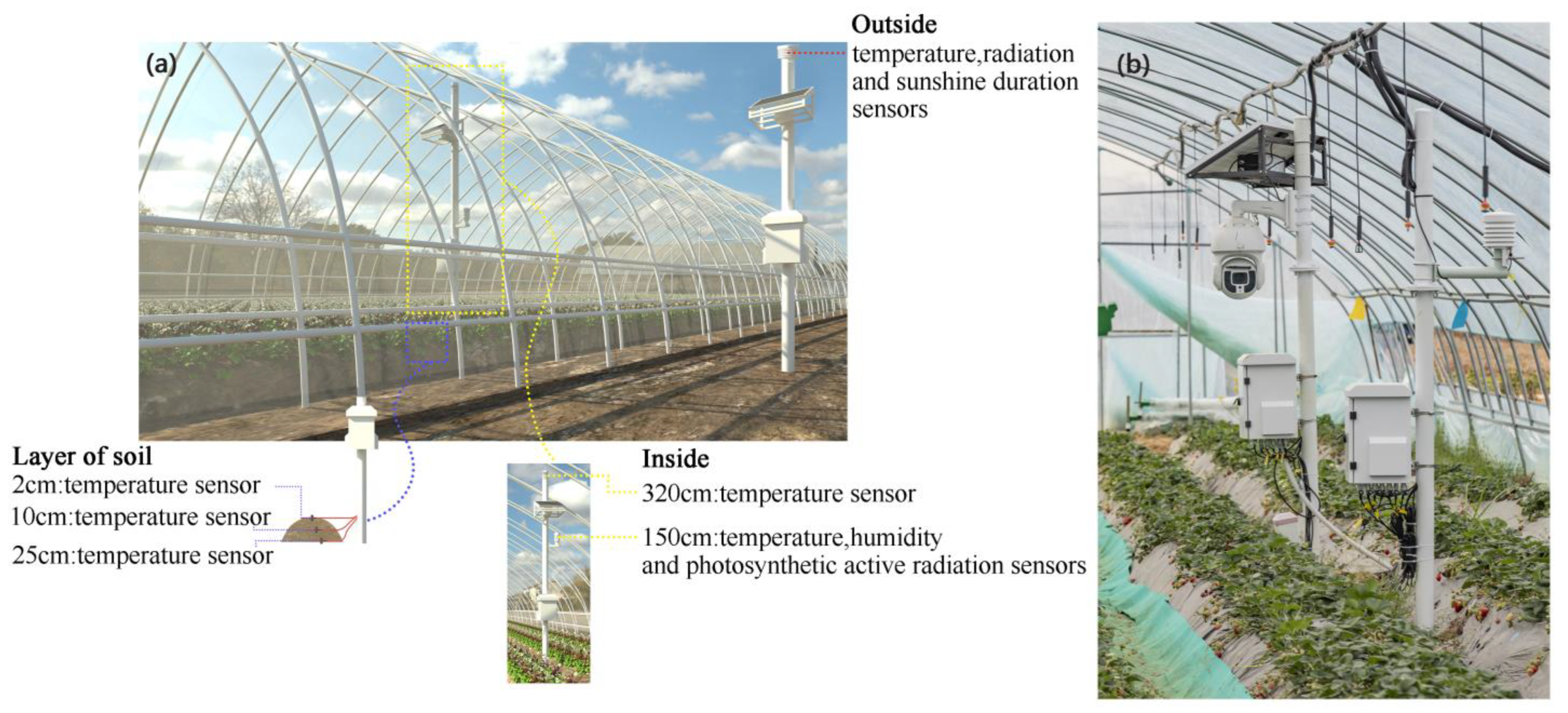
2.2. Data Collection Inside and Outside the Plastic Greenhouse

The experiment was conducted at the Hefei Agrometeorological Experimental Station from September 2021 to March 2023. In plastic greenhouses for strawberry cultivation, Microclimate Gradient Observing System (MGOS) as integrated by Anhui Lanke Information Technology Co. (Hefei, Anhui Province), with temperature and humidity sensors and photosynthetically active radiation sensors of HMP155 and SQ-421, respectively. The MGOS was installed, with the implementation of continuous and automatic monitoring of various meteorological elements for soil temperature at a depth of 25 cm (T_s25), soil temperature at a depth of 10 cm (T_s10), soil temperature at a depth of 2 cm (T_s2), air temperature at a height of 150 cm (T_a150), relative humidity at a height of 150 cm (RH₁₅₀), photosynthetic active radiation at a height of 150 cm (PAR₁₅₀), relative humidity at a height of 320 cm (RH₃₂₀), and air temperature at a height of 320 cm (T_a320)_. The relevant variables are shown in

Table 1. Various meteorological observation elements inside and outside plastic greenhouses for strawberry cultivation.

No.	Variable	Abbreviation	Unit
1	Soil temperature at a depth of 25 cm	Ts25	°C
2	Maximum soil temperature at a depth of 25 cm	Tsmax25	°C
3	Minimum soil temperature at a depth of 25 cm	Tsmin25	°C
4	Mean soil temperature at a depth of 25 cm	Tsmean25	°C
5	Mean soil temperature of one day before at a depth of 25 cm	Tsmean25odb	°C
6	Mean soil temperature of two days before at a depth of 25 cm	Tsmean25tdb	°C
7	Soil temperature at a depth of 10 cm	Ts10	°C
8	Maximum soil temperature at a depth of 10 cm	Tsmax10	°C
9	Minimum soil temperature at a depth of 10 cm	Tsmin10	°C
10	Mean soil temperature at a depth of 10 cm	Tsmean10	°C
11	Mean soil temperature of one day before at a depth of 10 cm	Tsmean10odb	°C
12	Mean soil temperature of two days before at a depth of 10 cm	Tsmean10tdb	°C
13	Soil temperature at a depth of 2 cm	Ts2	°C
14	Maximum soil temperature at a depth of 2 cm	Tsmax2	°C
15	Minimum soil temperature at a depth of 2 cm	Tsmin2	°C
16	Mean soil temperature at a depth of 2 cm	Tsmean2	°C
17	Mean soil temperature of one day before at a depth of 2 cm	Tsmean2odb	°C
18	Mean soil temperature of two days before at a depth of 2 cm	Tsmean2tdb	°C
19	Air temperature at a height of 150 cm	Ta150	°C
20	Maximum air temperature at a height of 150 cm	Tamax150	°C
21	Minimum air temperature at a height of 150 cm	Tamin150	°C
22	Mean air temperature at a height of 150 cm	Tamean150	°C
23	Mean air temperature of one day before at a height of 150 cm	Tamean150odb	°C
24	Mean air temperature of two days before at a height of 150 cm	Tamean150tdb	°C
25	Relative humidity at a height of 150 cm	RH150	%
26	Maximum relative humidity at a height of 150 cm	RHmax150	%
27	Minimum relative humidity at a height of 150 cm	RHmin150	%
28	Photosynthetic active radiation at a height of 150 cm	PAR150	μmol m−2 day−1
29	Air temperature at a height of 320 cm	Ta320	°C
30	Maximum air temperature at a height of 320 cm	Tamax320	°C
31	Minimum air temperature at a height of 320 cm	Tamin320	°C
32	Mean air temperature at a height of 320 cm	Tamean320	°C
33	Mean air temperature of one day before at a height of 320 cm	Tamean320odb	°C
34	Mean air temperature of two days before at a height of 320 cm	Tamean320tdb	°C
35	Relative humidity at a height of 320 cm	RH320	%
36	Maximum relative humidity at a height of 320 cm	RHmax320	%
37	Minimum relative humidity at a height of 320 cm	RHmin320	%
38	Outdoor maximum air temperature	Toamax	°C
39	Outdoor minimum air temperature	Toamin	°C
40	Outdoor mean air temperature	Tamean	°C
41	Outdoor sunshine duration	SD	hour
42	Outdoor solar radiation energy	Sre	W/m2

Note: T_a320 and RH₃₂₀ indicated the value of temperature and humidity between the two layers of the plastic film, respectively.

below. The MGOS was installed at 1/3 of one side of the plastic greenhouse (Figure 2). The simultaneous meteorological observations outside the plastic greenhouses were obtained from the National Ground Meteorological Observatory (NGMO) at a horizontal distance of 30 m from the experimental area, and the height of the roof of the greenhouses was equidistant from the ground observation field. Observational elements acquired include temperature, hours of sunshine, solar radiant energy (in the range 0–2000 W/m²), etc. All environmental data are collected in real time, quality controlled, and automatically transferred to a local server. The data set was then subjected to manual quality control in two steps before analysis: first, the data period was selected from September to March of the following year; second, data with daily absences of more than 3 h were excluded and data from stations with absences of less than 3 h were interpolated. After quality control, 382 days of daily and hourly data were available for modelling and validation.

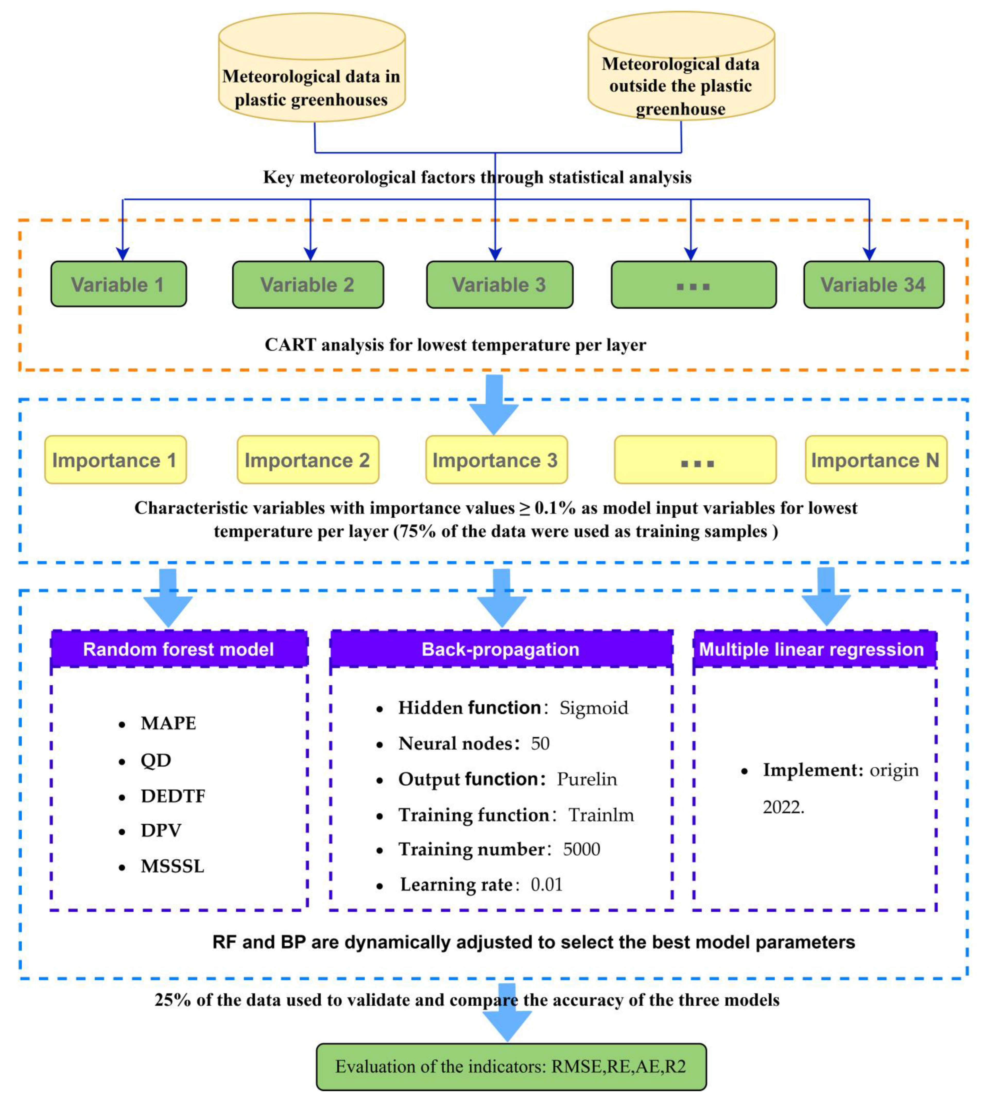
2.3. Predication Models

In this study, RF, BP, and MLR were employed to predict minimum temperature values at different depths and heights, whereas CART was applied to identify the main meteorological factors controlling minimum temperatures at different depths and heights. CART is a non-parametric data mining technique that can reflect non-linear and non-additive relationships between the response variable and predictor variables [28,29,30,31,32]. RF is able to significantly improve the prediction accuracy of the model compared to CART by integrating learning, feature randomness, and noise reduction [33]. The sample data set for the RF consists of key meteorological factors inside and outside the plastic greenhouses that affect minimum temperatures at different depths and heights. First, the training set and the test set are extracted by the random sampling method, and then the N subsets needed to construct N trees are obtained by sampling from the original sample set by the self-help method, and the data that are not sampled each time are called out-of-bag data, which are used to perform the estimation of the internal error and the evaluation of the importance of the feature variables. Details of the implementation of the random forest algorithm can be found in the literature [23,34]. BP is a multi-layer feed-forward network. It is trained using the error back-propagation algorithm. In this study, the gradient search technique is used to continuously adjust the weights and thresholds of the network through back-propagation to achieve the minimisation of the mean square deviation between the actual and desired outputs of the network. This paper adopts a 3-layer topology, which is set up based on the number of input layers [35,36]. MLR is a classical approach that has been widely used to predict the values of a dependent variable from predictor variables. It explores how the dependent and independent variables are correlated. In this study, RF and BP were implemented using the Python 3.12 programming language and MLR was implemented using Origin 2022. Schematic diagram of the three methods for predicting minimum temperatures at different depths and height layers of plastic greenhouses is shown in Figure 3 below.

2.4. Model Accuracy Evaluation Methods

In this study, Mean Absolute Percentage Error (MAPE), Root Mean Squared Error (RMSE), Relative Prediction Error (RE), Absolute Error (AE), and Coefficient of Determination (COD) R² were used to analyse and evaluate the agreement between simulated and measured minimum temperatures of plastic greenhouses in different depth and height layers as shown in Equations (1)–(5).

$$\mathrm{M}\mathrm{A}\mathrm{P}\mathrm{E}=(1/n)\times {\displaystyle \sum _{i=1}^n(\frac{\left|\right(O_i-S_i\left)\right|}{O_i})}\times 100\%$$

(1)

$$\mathrm{R}\mathrm{M}\mathrm{S}\mathrm{E}=\sqrt{{\displaystyle \frac{{\displaystyle \sum _{i=1}^n{(O_i-S_i)}^2}}{n}}}$$

(2)

$$\mathrm{R}\mathrm{E}={\displaystyle \frac{{\displaystyle \sum _{i=1}^n\left|\frac{S_i-O_i}{O_i}\right|}}{n}}$$

(3)

$$\mathrm{A}\mathrm{E}={\displaystyle \frac{{\displaystyle \sum _{i=1}^n\left|S_i-O_i\right|}}{n}}$$

(4)

$${\mathrm{R}}^2={\displaystyle \frac{{\left[{\displaystyle \sum _{i=1}^n\left(S_i-\overline{S}\right)\left(O_i-\overline{O}\right)}\right]}^2}{{\displaystyle \sum _{i=1}^n{(S_i-\overline{S})}^2{\displaystyle \sum _{i=1}^n{\left(O_i-\overline{O}\right)}^2}}}}$$

(5)

In the equation, S_i represents the predicted value; O_i represents the actual value; n represents the number of validation samples.

3. Results

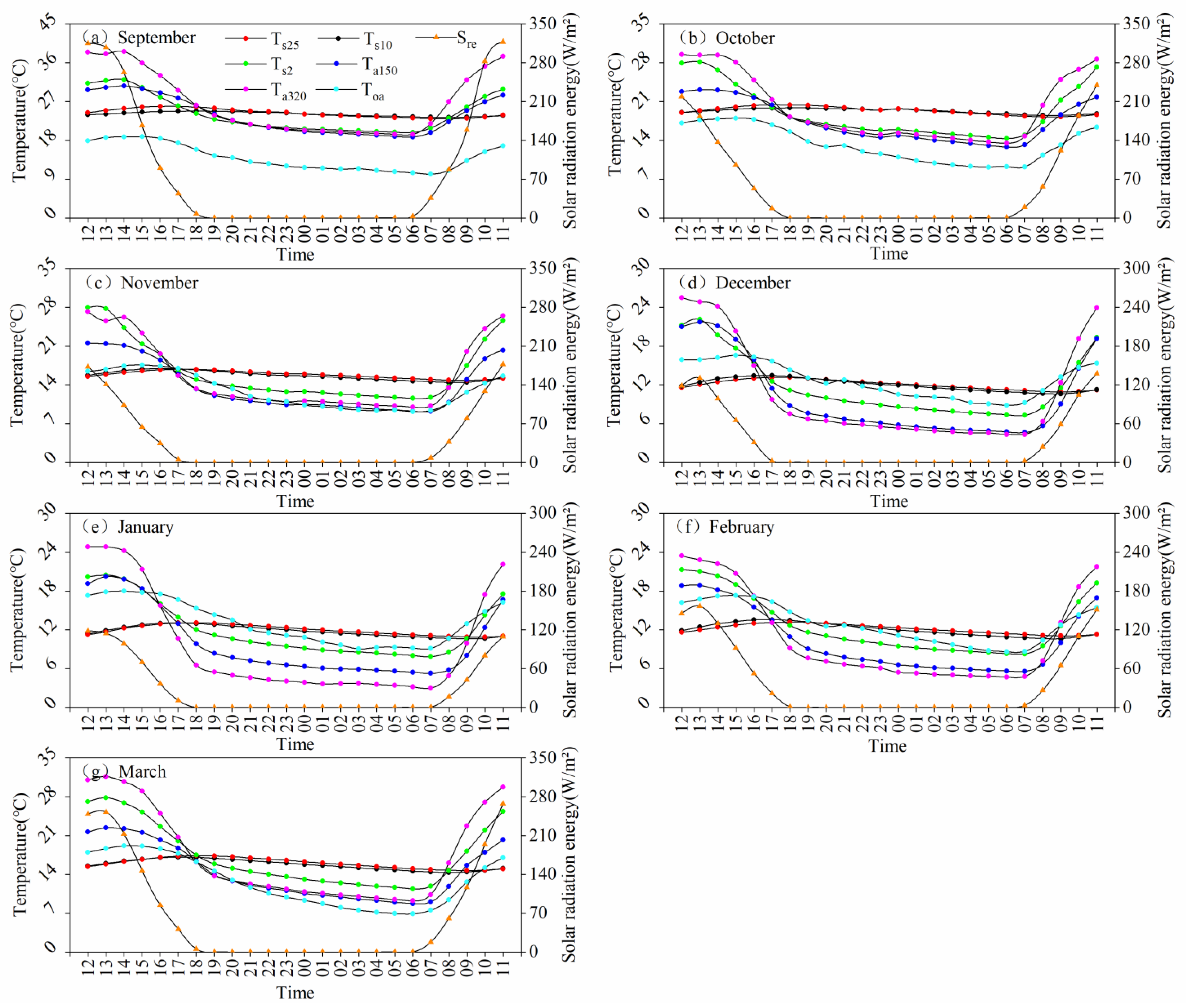
3.1. Characteristics of Monthly and Hourly Mean Temperature and Mean Solar Energy Variations in Different Depths and Heights at Plastic Greenhouses for Strawberry Cultivation

Figure 4a–g showed the daily temperature profiles of layered temperature and solar energy variations at different depths and heights inside and outside the plastic greenhouses during different strawberry growing seasons. Each hourly temperature and solar energy data are taken from the average of the corresponding hourly data for each day from the 1st to the end of the month. As can be seen from Figure 4 below, the temperature changes in the 25 cm and 10 cm soil layers in different months were the smallest, the curve fluctuated more smoothly, there was a slower recovery of soil temperature during the daytime hours. Peak soil temperatures in different layers occurred later relative to the inside of the plastic greenhouse at 150 cm and 320 cm and air temperatures outside the plastic greenhouse. The value of solar radiation energy is basically zero from 17:00 to 7:00, and it reaches its maximum between 11:00 and 13:00. From September to March of the following year, soil temperatures at 10 cm stabilised above 11.8 degrees Celsius on a monthly average. The air temperature inside and outside the plastic greenhouses for strawberry cultivation basically showed a trend of increasing and then decreasing at different heights in different months, with the daily change in temperature range of T_a320 > T_a150 > T_oa. During the day, the temperature at 320 cm (between the two layers of plastic film) was significantly higher than the temperature at 150 cm and outside the plastic greenhouse, and the night temperature was characterised by significant seasonal variations. Minimum temperatures at different depths and heights generally occur around 6:00–7:00 am, with slight variations from month to month. The analysis in Figure 4 also showed that in September and March of the following year there were periods of high temperatures above 30 °C at the 320 cm level of the plastic greenhouse, which shows a higher risk of high temperature heat damage, which accelerated or delayed strawberry development to varying degrees [37].

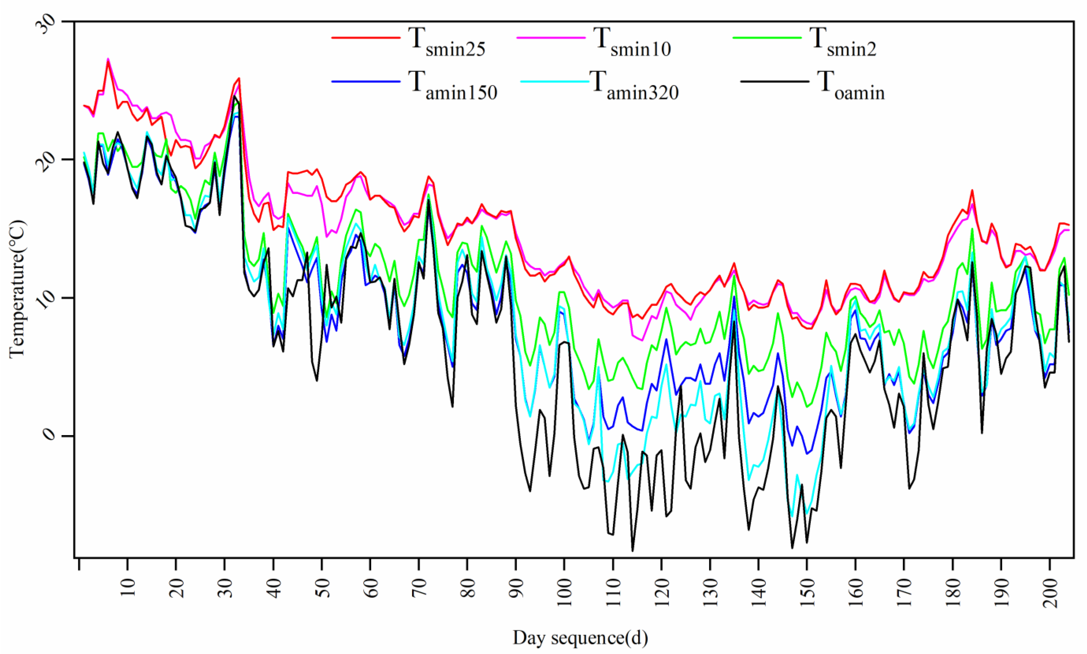
3.2. Characteristics of Daily Variation in Minimum Temperature in Different Depths and Heights of Plastic Greenhouse for Strawberry Cultivation

Figure 5 showed the characteristic daily profiles of minimum temperature changes in different depths and heights during the strawberry growing season. From the figure, it can be seen that the minimum temperature values of the 10 cm and 25 cm soil layers are significantly higher than the air temperature values of the different height layers inside and outside the plastic greenhouses on the same day. From November to the following March, the daily minimum temperature in the plastic greenhouses at heights of 150 cm and 320 cm appeared to be consistently lower than −5 °C. Sometimes the lowest temperatures at 150 cm and 320 cm were as low as −1.3 °C and −6.2 °C, respectively. At this time, strawberry is in the critical period of flowering and fruiting, and persistent low-temperature frost directly affects the flowering and fruiting of strawberry and the yield formation, which means that during this key stage, plastic greenhouses must be environmentally regulated. Therefore, it is of great importance to systematically study the change rule of minimum temperature in different depths and heights of plastic greenhouses and guide local farmers to carry out the defence of low-temperature freezing of strawberries.

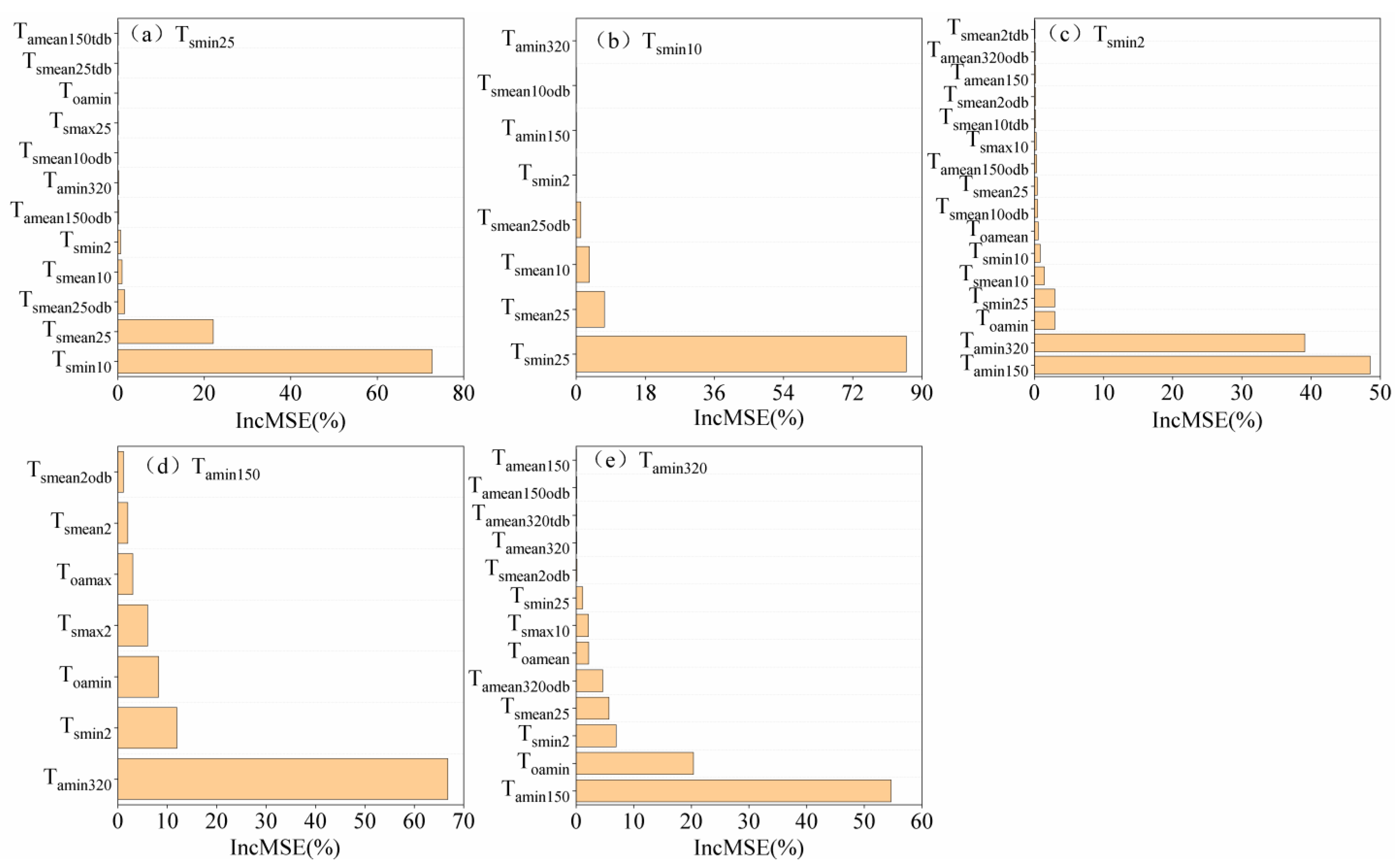
3.3. Analysis of the Importance of Variables Characterising Different Meteorological Elements in Plastic Greenhouse for Strawberry Cultivation

The results of the previous study showed that changes in various meteorological conditions inside and outside the plastic greenhouses were the main factors affecting the minimum temperature at different depths and heights inside the plastic greenhouses. In addition, the changes in the temperature of the air layer at different heights and the soil layer at different depths yesterday and the day before were also key factors influencing the changes in the minimum temperature of the day, with a significant lag effect. So, with so many key meteorological variables, what are the most critical factors affecting the prediction of minimum temperatures in different depths and heights of plastic greenhouses, and how should one judge which ones to choose as input variables? This is a question worth investigating. For this purpose, 34 variables were selected at different depths and heights inside and outside the plastic greenhouse as input variables, covering various meteorological elements such as minimum temperature, maximum temperature, average temperature, average temperature of the previous 1 day, average temperature of the previous 2 days, radiation at the height of 150 cm and temperature and sunshine hours (Table 1). The CART was used to predict the importance of each variable at different depths and heights of minimum temperature, and the importance of the characteristic variables is shown in Figure 6. The results of CART revealed that the key variables affecting the minimum temperature at different depths and heights were significantly different. T_smin10 was the most important variable for explaining the variation in T_smin25. The T_smean25 was the second most important variable controlling T_smin25 dynamics. The remaining variables, e.g., T_smean25odb, T_smean10, T_smin2, T_amean150odb, T_amin320, T_smean10odb, T_smax25, T_oamin, T_smean25tdb, and T_amean150tdb were the least important factors for T_smin25 dynamics. By analogy, the most important variables influencing the variation in minimum temperatures in the 10 cm depth, 2 cm depth, 150 cm, and 320 cm height layers are the 25 cm depth minimum temperature, the 150 cm minimum temperature, the 320 cm minimum temperature, and the 150 cm minimum temperature, respectively. By analogy, the most important variables that affect the changes in T_smin10, T_smin2, T_amin150, and T_amin320 were T_smin25, T_amin150, T_amin320, and T_amin150, respectively. The second most important variables were T_smean25, T_amin320, T_smin2, and T_oamin, respectively. Statistical analysis of the importance of the characteristic variables showed that the first two variables have an explanatory rate of 94.85 per cent, 93.4 per cent, 87.64 per cent, 78.82 per cent, and 75.07 per cent, respectively. This suggests that the first two are the most important factors influencing the variation in minimum temperatures at different depths and heights.

3.4. Construction of the Minimum Temperature Forecast Model in Different Depths and Heights of Plastic Greenhouse for Strawberry Cultivation

In order to obtain highly accurate models for the prediction of minimum temperatures in different depths and heights of plastic greenhouse, RF, BP, and MLR were used to train the data. The 382 valid data were screened by quality control; 75% of the data were used as training samples and 25% of the data were used for accuracy testing. In this paper, based on the results of the above analysis of the importance of the minimum temperature characteristic variables, the variables with an importance of the characteristic variables higher than 0.1 per cent were selected as input variables for the model. In this paper, the MAPE metrics were used to evaluate the models after building 1000 decision trees. The quasi-differences (QD) in the decision tree model parameters were preset as RMSE or AE. The depth of each decision tree in the forest (DEDTF) is set by default to 8, 9, 10, or 11. The default number of decision trees (DNDT) is 15, 16, or 17. The default percentage of variables (DPV) used per decision tree was 0.3, 0.4, or 0.5. The minimum split sample size for leaves (MSSSL) defaulted to 4, 8, 12. The minimum temperatures of different depths and heights were used as output variables, while the default values of the variables in the decision tree were dynamically adjusted according to the MAPE values, and the best parameters were finally selected. In this paper, the minimum temperature prediction model is developed separately using RF, and the relevant input parameters are shown in

Table 2. Optimal parameters for RF model selection.

Tmin	QD	MAPE	DEDTF	DPV	MSSSL	DNDT
Tsmin25	AE	1.87	13	0.7	4	17
Tsmin10	RMSE	3.56	9	0.5	4	19
Tsmin2	AE	6.93	7	0.7	4	17
Tamin150	RMSE	4.25	12	0.7	4	19
Tamin320	RMSE	16.51	13	0.6	4	17

Note: T_min: minimum temperature; QD: quasi-differences; MAPE: Mean Absolute Percentage Error; DEDTF: Depth of each decision tree in the forest; DPV: Default percentage of variables; MSSSL: Minimum split sample size for leaves; DNDT: Default number of decision trees.

below. A minimum temperature prediction model based on the BP is developed in the following steps: The filtered feature variables affecting the minimum temperature (Figure 6) were first normalised and used as input layers. The network was then trained on the impact factor data set. Sigmoid function is used for the hidden layer neuron transfer function. The number of variables in the net of neural nodes is set to 50 according to the number of predictor factors. The Purelin function is used for the transfer function of the output layer neuron. The training function used was Trainlm, with a training number of 50,000 and an initial learning rate of 0.01. The data were trained using the MLR in Origin 2024 and its multiple linear regression equation and R² are shown in

Table 3. Multiple linear regression equation for minimum temperature in different depths and heights of plastic greenhouses for strawberry cultivation.

Variables	Multiple Regression Equation	R2
Tsmin25	y = 0.172 × Tsmin10 − 0.096 × Tsmean10 + 0.033 × Tsmean10odb − 0.417 × Tsmax25 + 1.166 × Tsmean25 + 0.012 × Tsmean25odb + 0.004 × Tsmean25tdb + 0.108 × Tsmin2 + 0.003 × Tamin320 − 0.026 × Tamean150 + 0.012 × Tamean150tdb + 0.005 × Toamin + 0.433	0.994 **
Tsmin10	y = 0.167 × Tsmean10 + 0.134 × Tsmean10odb + 1.237 × Tsmin25 − 0.231 × Tsmean25 − 0.106 × Tsmean25odb − 0.429 × Tsmin2 − 0.045 × Tamin320 + 0.302 × Tamin150 − 0.518	0.969 **
Tsmin2	y = − 0.294 × Tsmax10 − 0.752 × Tsmin10 + 0.894 × Tsmean10 − 0.028 × Tsmean10odb + 0.056 × Tsmean10tdb + 0.822 × Tsmin25 − 0.480 × Tsmean25 − 0.025 × Tsmean2 + 0.185 × Tsmean2odb − 0.07 × Tamin320 − 0.145 × Tamean320odb + 0.630 × Tamin150 + 0.079 × Tamean150 + 0.002 × Tamean150 + 0.033 × Toamin + 0.050 × Toamean + 1.116	0.957 **
Tamin150	y = 0.005 × Tsmax2 + 0.836 × Tsmin2 − 0.027 × Tsmean2 − 0.099 × Tsmean2odb + 0.284 × Tamin320 − 0.025 × Toamax + 0.047 × Toamin − 1.137	0.955 **
Tamin320	y = 0.129 × Tsmax10 + 0.056 × Tsmin25 − 0.281 × Tsmean25 − 0.186 × Tsmin2 − 0.086 × Tsmean2odb + 0.256 × Tamean320 + 0.205 × Tamean320odb + 0.034 × Tamean320tdb + 1.148 × Tamin150 − 0.494 × Tamean150 − 0.180 × Tamean150 + 0.097 × Toamin + 0.171 × Toamean + 1.753	0.971 **

Note: ** indicates significance of difference at 0.01 level.

below.

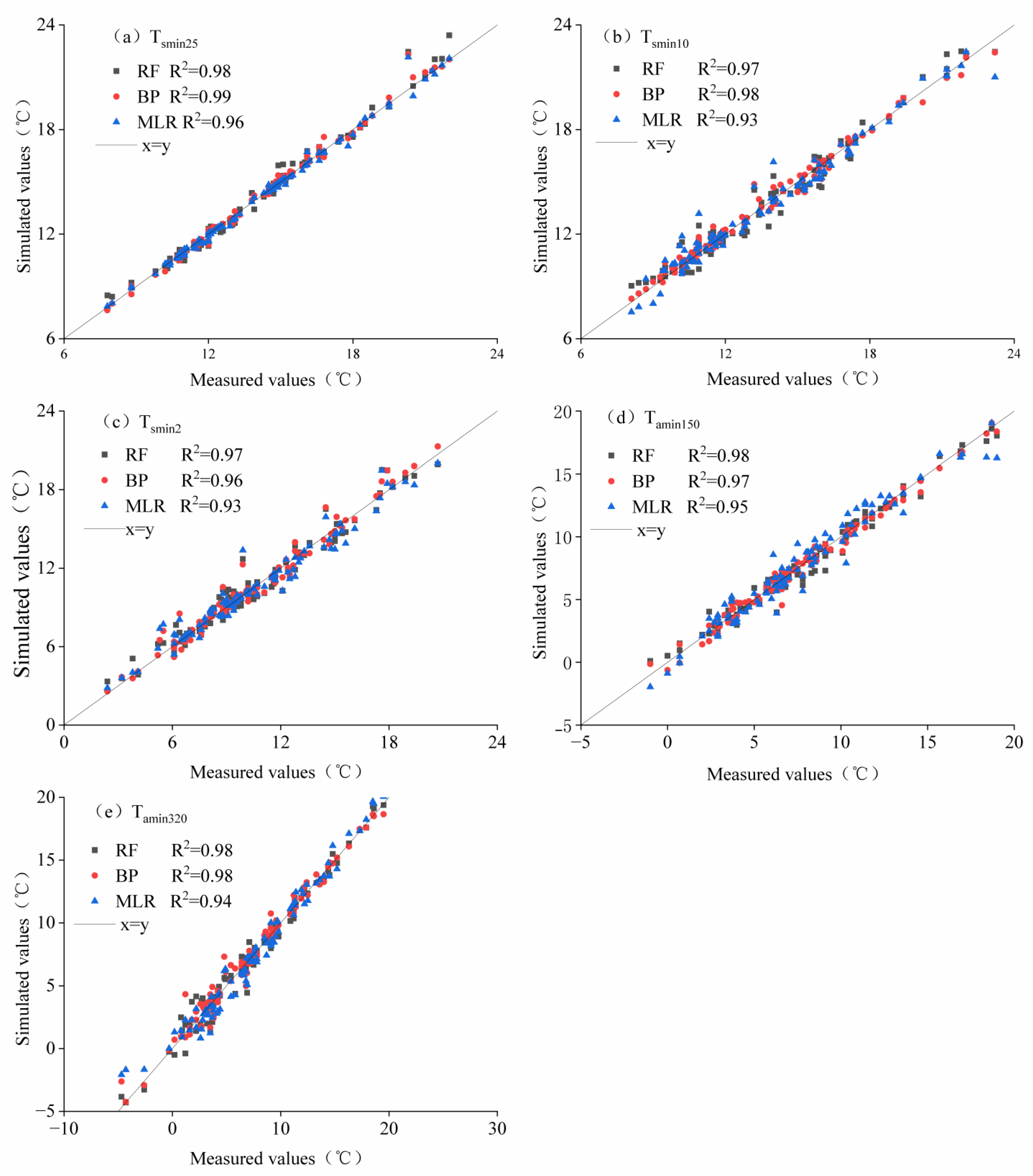
3.5. Model Validation for Predicting Minimum Temperatures in Different Depths and Heights of Plastic Greenhouses for Strawberry Cultivation

The simulated values of minimum temperatures at different depths and heights of plastic greenhouses predicted by the RF, BP, and MLR were analysed in comparison with the measured values for the same period. The results are shown in Figure 7, where the simulated and measured minimum temperatures at different depths and heights are relatively evenly distributed around the 1:1 line. The coefficients of determination of the simulated and measured minimum temperatures at different depths and heights were higher than 0.93 for all three models, and the coefficients of determination of the RF and the BP were higher than those of the MLR. The prediction test with different depths and heights of minimum temperature in plastic greenhouses is shown in

Table 4. Model validation for minimum temperatures at different depths and heights.

	Forecasting Methods	RMSE (°C)	RE (%)	AE (°C)	R2
Tsmin25	RF	0.37	0.02	0.25	0.98
	BP	0.31	0.01	0.19	0.99
	MLR	0.27	0.01	0.16	0.96
Tsmin10	RF	0.62	0.04	0.46	0.97
	BP	0.48	0.02	0.30	0.98
	MLR	0.61	0.03	0.44	0.93
Tsmin2	RF	0.85	0.07	0.65	0.97
	BP	0.81	0.06	0.54	0.96
	MLR	0.80	0.06	0.54	0.93
Tamin150	RF	0.61	0.03	0.45	0.98
	BP	0.78	0.04	0.45	0.97
	MLR	0.91	0.04	0.69	0.95
Tamin320	RF	0.68	0.21	0.53	0.98
	BP	0.74	0.24	0.51	0.98
	MLR	0.86	0.29	0.67	0.94

and Figure 8. The comparison of RMSE, RE, and AE values showed that RF is higher than BP and MLR in predicting the minimum temperature at −25 cm, −10 cm, and −2 cm depths, but the opposite trend is shown at 150 cm and 320 cm heights, i.e., RF is better than BP model and MLR. The three models simulated the minimum temperature at 320 cm height with significantly higher RE values than those at different depths of the soil layer and at 150 cm height.

The results of the above analyses showed that the simulation of the minimum temperature using RF, BP and MLR all had excellent performance. Overall, the RF and BP were superior to the MLR. The RF and BP were more effective in exploring the intricate relationships between different weather elements inside and outside the plastic greenhouses. The results also showed that for different depths and heights inside the plastic greenhouses, the selection of appropriate models can significantly improve the accuracy of predicting the minimum temperature of the plastic greenhouses so as to scientifically carry out the fine control of the plastic greenhouses and provide a scientific basis for the prevention and mitigation of strawberry disasters.

4. Discussion

Low temperature stress not only affects the chlorophyll content, photosystem fluorescence, protective enzymes, stomatal characteristics, and pollen development of strawberry leaves, but also reduces pollination success, numbers of fruit sets, and affects fruit yield and quality [38,39,40,41]. In practice, strawberries are often exposed to varying degrees of low temperature stress. The most critical developmental period in strawberry production is the flowering and fruiting period, and prolonged low-temperature freezing will prolong the developmental process of strawberry and even cause a large-scale reduction in the strawberry crop phenomenon. Therefore, based on extensive knowledge of the actual situation of strawberry greenhouse cultivation in the Changfeng area, we selected the widely planted “Red Face” as the research object. Field observation experiments of various meteorological elements in different depths of soil layers and different height layers in plastic greenhouses were carried out with the aim of exploring the characteristics of minimum temperature changes in different depths and heights in plastic greenhouses and establishing a prediction model of minimum temperature in plastic greenhouses based on the theoretical basis, so as to provide a scientific basis for the defence of low temperature freezing of strawberries in actual production.

The main function of horticultural facilities is to provide suitable environmental conditions for crops, the most important of which are temperature, light, and humidity conditions, and proper environmental control of facilities can effectively reduce the incidence of low temperature, low light, pests, and other meteorological disasters in facility crops. The growth cycle of strawberry is divided into five distinct stages: stolonogenesis, seedling, bud differentiation, flowering and fruiting, and dormancy. The growth of the strawberry is closely related to the environmental conditions, which are favourable with a temperature of 10–30 °C, with an optimal temperature of 15–25 °C. Below 10 °C is when the flower bud differentiation stopped. If the temperature of the environment in which the strawberry is growing drops significantly, the leaves of the whole plant will turn dark green and will wilt in a water-soaked state [42]. Strawberries in full bloom are most sensitive to low temperatures, and prolonged low temperatures and low sunlight can easily lead to frozen buds or poor fertilisation, resulting in flowers but no fruit [43]. The large amount of data in this study confirmed that the daily variation in soil temperature at different depths was more stable with two layers of plastic sheeting, with the lowest temperatures occurring between 6:00 and 7:00 am. From September to the following March, the average temperature of the 10 cm soil reached 24, 19.3, 15.7, 12, 11.8, 12, 15.7 °C, while the average temperature of the 25 cm soil reached 24.3, 19.3, 15.8, 12, 11.9, 12.1, 16 °C, respectively. The results of the study showed that strawberries grown inside the two layers of film did not suffer from root freezing, but they grew more slowly because the temperature did not reach 15 °C. From the daily variation in the lowest air temperature layer by layer in the plastic greenhouse, after two layers of the greenhouse film cover, there was a low temperature freeze of −5.8 °C in winter, electrolytes appeared as an obvious extravasation phenomenon, and the photosynthetic capacity was significantly reduced [44].

Secondly, the input parameters of the prediction model are the basis for determining the accuracy of minimum temperature prediction at different depths and heights. In this paper, based on the results of the importance analysis of the characteristic variables, the final numbers of input variables screened for different depths and heights were 12, 8, 16, 7, and 13, respectively. Based on the above key meteorological factors, RF, BP, and MLR were used to achieve the prediction of minimum temperatures in different depths and heights of plastic greenhouses, respectively. All three models showed some predictive potential when tested with independent data. The predictive accuracy of MLR is lower than that of RF and BP, indicating that machine learning algorithms are superior to traditional forecasting methods that build regression equations for single or multiple meteorological factors. Taken together, the idea of using machine learning algorithms to build minimum temperature prediction models for different depths and heights of plastic greenhouses in this paper provides a new approach to predicting low temperature freezing of strawberries in winter and spring. The analysis and comparison of the simulation accuracy of RF, BP, and MLR can provide a scientific basis for selecting different prediction models for different depths and heights of plastic greenhouses.

The conclusions of this study are based on the ‘Productive Plastic Greenhouses’ and ‘Red Face’ studies, and whether more types of greenhouse and strawberry cultivars show patterns of low-temperature chilling injury that are all consistent with the conclusions drawn in this study, or whether the minimum temperature prediction model needs further adjustment and optimisation, all need to be tested and improved by continuing to conduct more strawberry cultivars and more types of greenhouse experiments in the future.

5. Conclusions

The characteristics of the daily change in layer-by-layer temperature in plastic greenhouses in different months were similar, and the daily difference in soil temperature in different depths was smaller than the daily difference in air temperature in different heights, and even though there were two layers of plastic greenhouses covering the situation, strawberries in greenhouses were still exposed to different degrees of low-temperature frost damage in winter. Therefore, winter is the key to environmental control of strawberries in Changfeng area, and other auxiliary warming measures can be taken appropriately to avoid the occurrence of low-temperature frost damage and increase the yield and quality of strawberries.

There were more important meteorological factors affecting the minimum temperature of different depths and heights of plastic greenhouses, and this paper used the CART algorithm in the RF model to analyse the importance of the characteristic variables of each meteorological factor, which can greatly reduce the number of input variables. It is difficult to explain the complex non-linear relationship between response variables and predictor variables using the traditional regression model; compared with the traditional regression model, RF and BP deal with non-linear and hierarchical relationships more obvious advantages.

The coefficient of determination of all three models in simulating minimum temperatures at different depths and different heights was high, and the comparison of RMSE and RE values showed that the prediction error of RF was higher than that of BP and MLR at different depths of the soil layer, but it showed an opposite trend at different heights of the plastic greenhouses.

References

1. Song, C. Quality Strawberry Greenhouse Pollution-free Cultivation Technology. Agric. Eng. Technol. 2021, 41, 79–81. [Google Scholar]
2. Carbone, F.; Preuss, A.; DeVos, R.C.H.; D’Amico, E.; Perrotta, G.; Bovy, A.G.; Martens, S.; Rosati, C. Developmental, genetic and environmental factors affect the expression of flavonoid genes, enzymes and metabolites in strawberry fruits. Plant Cell Environ. 2009, 32, 1117–1131. [Google Scholar] [CrossRef] [PubMed]
3. Xu, Y. Strawberry High-yield Cultivation Technology. Rural. Sci. Technol. 2021, 12, 70–71. [Google Scholar]
4. Wang, S.Y.; Camp, M.J. Temperatures after bloom affect plant growth and fruit quality of strawberry. Sci. Hortic. 2000, 85, 183–199. [Google Scholar] [CrossRef]
5. Li, Q.; Shen, S.; Cao, W.; Zou, X. Neural Network Simulation on Air Temperature and Relative Humidity inside Plastic Greenhouse during Winter and Spring in Southern China. Chin. J. Agrometeorol. 2012, 33, 190–196. [Google Scholar]
6. Businger, J.A. The Glasshouse Climate Physics of Plant Environment; North-Holland Publishing Company: Amsterdam, The Netherlands, 1963; pp. 277–318. [Google Scholar]
7. Yang, D.; Ding, H.; Sun, J.; Li, Q.; Wei, S.; Huang, H. Characteristics and Forecasting Technology of Greenhouse Temperature Deficit in Southern Plastic Greenhouse. Chin. J. Agrometeorol. 2019, 40, 240–249. [Google Scholar]
8. Li, Q.; Shen, H.; Tao, S.; Zou, X. Simulation of Daily Air Temperature Inside Plastic Greenhouse Based on Harmonic Method. Chin. J. Agrometeorol. 2014, 35, 33–41. [Google Scholar]
9. Li, D.; Zhang, X.; Qi, H.; Zhang, B. Forecast Model of the Highest and Lowest Temperature in the Sunlight Greenhouse in Suzhou. Chin. J. Agrometeorol. 2013, 34, 170–178. [Google Scholar]
10. Abdel-Ghany, A.M.; Kozai, T. Dynamic modeling of the environment in a naturally ventilated, fog-cooled greenhouse. Renew. Energy 2006, 31, 1521–1539. [Google Scholar] [CrossRef]
11. Kumar, A.; Tiwari, G.N. Thermal modeling of a natural convection greenhouse drying system for jaggery: An experimental validation. Sol. Energy 2006, 80, 1135–1144. [Google Scholar] [CrossRef]
12. Fidaros, D.K.; Baxevanou, C.A.; Bartzanas, T. Numerical simulation of thermal behavior of a ventilated arc greenhouse during a solar day. Renew. Energy 2010, 35, 1380–1386. [Google Scholar] [CrossRef]
13. Okushima, L.; Sase, S.; Nara, M.A. support system for natural ventilation design of greenhouses based on computational aerodynamics. Acta Hortic. 1989, 284, 129–136. [Google Scholar] [CrossRef]
14. Kacira, M.; Sase, S.; Okushima, L. Effects of side vents and span numbers on wind-induced natural ventilation of agothic multi-span greenhouse. Jpn. Agric. Res. Q. 2004, 38, 227–233. [Google Scholar] [CrossRef]
15. Su, W.; Xue, X.; Xiong, Y.; Cao, J. Modeling the effect of natural ventilation on temperature inside solar greenhouse. Chin. J. Ecol. 2016, 35, 1635–1642. [Google Scholar]
16. Frausto, H.U.; Pieters, J.G.; Deltour, J.M. Modelling greenhouse temperature by means of auto regressive models. Biosyst. Eng. 2003, 84, 147–157. [Google Scholar] [CrossRef]
17. Herrero, J.M.; Blasco, X.; Martínez, M.; Ramos, C.; Sanchis, J. Non-linear robust identification of a greenhouse model using multi-objective evolutionary algorithms. Biosyst. Eng. 2007, 98, 335–346. [Google Scholar] [CrossRef]
18. Morteza, T.; Yahya, A.; Seyed, F.R. Modeling and experimental validation of heat transfer and energy consumption in an innovative greenhouse structure. Inf. Process. Agric. 2016, 3, 57–174. [Google Scholar]
19. Du, S.; Li, Y.; Chen, L.; Li, J. Modelling Greenhouse Environment with Artifical Neural Networks. Comput. Meas. Control 2006, 14, 887–889. [Google Scholar]
20. Wang, D. SVM Regression Modeling for Greenhouse Environment. J. Agric. Mach. 2004, 35, 106–109. [Google Scholar]
21. Bai, L.; Xu, Y.; He, M.; Li, N. Remote Sensing Inversion of Near Surface Air Temperature Based on Random Forest. J. Geo-Inf. Sci. 2017, 19, 390–397. [Google Scholar]
22. Zhang, H.; Wu, P.; Yin, A.; Yang, X.; Zhang, M.; Gao, C. Prediction of soil organic carbon in an intensively managed reclamation zone of eastern China: A comparison of multiple linear regressions and the random forest model. Sci. Total Environ. 2017, 592, 704–713. [Google Scholar] [CrossRef] [PubMed]
23. Iverson, L.R.; Prasad, A.M.; Matthews, S.N.; Peters, M. Estimating potential habitat for 134 eastern US tree species under six climate scenarios. For. Ecol. Manag. 2008, 254, 390–406. [Google Scholar] [CrossRef]
24. Xu, M.; Zhao, Y.; Zhang, G.; Gao, P.; Yang, R. Method for forecasting winter wheat first flowering stage based on machine learning algorithm. Trans. Chin. Soc. Agric. Eng. (Trans. CSAE) 2021, 37, 162–171. [Google Scholar]
25. Li, D.; Chen, W.; Le, Z.; Fan, X.; Sun, Y.; Meng, Y.; Yang, J. Forecast method for the first flowering date of Dangshansu pear based on random forest algorithm and meteorological factors. Trans. Chin. Soc. Agric. Eng. (Trans. CSAE) 2020, 36, 143–151. [Google Scholar]
26. Xu, M.; Xu, J.; Xie, Z.; Gao, P.; Li, Y.; Miao, J. Application of the random forest machine algorithm in forecasting diseased panicle rate of wheat scab in Jiangsu province. Acta Meteorol. Sin. 2020, 78, 43–153. [Google Scholar]
27. Liu, J.; He, X.; Wang, P.; Huang, J. Early prediction of winter wheat yield with long time series meteorological data and random forest method. Trans. Chin. Soc. Agric. Eng. (Trans. CSAE) 2019, 35, 158–166. [Google Scholar]
28. Myles, A.J.; Feudale, R.N.; Liu, Y.; Woody, N.A.; Brown, S.D. An introduction to decision tree modeling. J. Chemom. A J. Chemom. Soc. 2004, 18, 275–285. [Google Scholar] [CrossRef]
29. De’Ath, G.; Fabricius, K.E. Classification and regression trees: A poweful yet simple technique for ecological data analysis. Ecology 2008, 81, 3178–3192. [Google Scholar] [CrossRef]
30. Teixeira, A. Analyse discrimante par arbre de décision binaire (CART: Classification And Regression Tree). Revue des Maladies Respiratoires. 2004, 21, 1174–1176. [Google Scholar] [CrossRef]
31. Wiesmeier, M.; Barthold, F.; Blank, B.; Kögelknabner, I. Digital mapping of soil organic matter stocks using random forest modeling in a semi-arid steppe ecosystem. Plant Soil 2011, 340, 7–24. [Google Scholar] [CrossRef]
32. Wiesmeier, M.; Munro, S.; Barthold, F.; Steffens, M.; Schad, P.; Kögel-Knabner, I. Carbon storage capacity of semi-arid grassland soils and sequestration potentials in northern China. Glob. Change Biol. 2015, 21, 3836–3845. [Google Scholar] [CrossRef]
33. Breiman, L. Random Forests. Mach. Learn. 2001, 45, 5–32. [Google Scholar] [CrossRef]
34. Prasad, A.M.; Iverson, L.R.; Liaw, A. Newer classification and regression tree techniques: Bagging and Random forests for ecological rediction. Ecosystems 2006, 9, 181–199. [Google Scholar] [CrossRef]
35. Cybenko, G. Approximation by superpositions of a sigmoidal function. Math. Control. Signals Syst. 1989, 2, 303–314. [Google Scholar] [CrossRef]
36. He, R.; Guan, Z.Y.; Jin, L.A. Short-term cloud forecast model by neural networks. Trans. Atmos. Sci. 2010, 33, 725–730. [Google Scholar]
37. Xu, C.; Wang, M.; Yang, Z.; Han, W.; Zheng, S. Effect of High Temperature in Seedling Stage on Phenological Stage of Strawberry and its Simulation. Chin. J. Agrometeorol. 2020, 41, 644–654. [Google Scholar]
38. Xu, R.; Yang, Z.; Sheng, M.; Wang, M. Effects of Low Temperature Stress at Seedling Stage on Chlorophyll Content and Canopy Hyperspectral of “Hongyan” Strawberry. Chin. J. Agrometeorol. 2022, 43, 148–158. [Google Scholar]
39. Xu, J.; Yang, Z.; Yuan, C.; Luo, J.; Wang, C.; Zhang, H.; Jiang, N. Effect of Low Temperature at Anthesis on the Fluorescence Properties of Photosystem and Protective Enzyme Activity of Strawberry Leaves. Chin. J. Agrometeorol. 2024, 45, 178. [Google Scholar]
40. Khammayom, N.; Maruyama, N.; Chaichana, C. The Effect of Climatic Parameters on Strawberry Production in a Small Walk-In Greenhouse. AgriEngineering 2022, 4, 104–121. [Google Scholar] [CrossRef]
41. Koehler, G.; Wilson, R.C.; Goodpaster, J.V.; Sønsteby, A.; Lai, X.; Witzmann, F.A.; You, J.S.; Rohloff, J.; Randall, S.K.; Alsheikh, M. Proteomic Study of Low-Temperature Responses in Strawberry Cultivars (Fragaria × ananassa) That Differ in Cold Tolerance. Plant Physiol. 2012, 159, 1787–1805. [Google Scholar] [CrossRef]
42. Wang, Y.; Yang, H.; Li, S. Research on Cold Damage and Cold Resistance in Horticultural Plants-A Review of Literature. Acta Hortic. Sin. 1994, 21, 239–244. [Google Scholar]
43. Hu, M.; Jin, C.; Pan, H. Impact of persistent rainy and sunny weather on strawberry production in early spring. Zhejiang Agric. Sci. 2012, 10, 1407–1409. [Google Scholar]
44. Jiang, N.; Yang, Z.; Zhang, H.; Xu, J.; Li, C. Effect of Low Temperature on Photosynthetic Physiological Activity of Different Photoperiod Types of Strawberry Seedlings and Stress Diagnosis. Agronomy 2023, 13, 1321. [Google Scholar] [CrossRef]
Figure 1. Comprehensive location map of plastic greenhouses used for the production of strawberries.
Agronomy 15 00709 g001
Figure 2. Microclimate gradient observation system in plastic greenhouses: (a) schematic; (b) actual site plan.
Agronomy 15 00709 g002
Figure 3. Schematic diagram of the three methods for predicting minimum temperatures at different depths and heights of plastic greenhouses.
Agronomy 15 00709 g003
Figure 4. Hourly temperature variation at different depths and heights in plastic greenhouses for strawberry cultivation. Ts25: Daily variation in soil temperature at a depth of 25 cm; Ts10: Daily variation in soil temperature at a depth of 10 cm; Ts2: Daily variation in soil temperature at a depth of 2 cm; Ta150: Daily variation in air temperature at a height of 150 cm; Ta320: Daily variation in air temperature at a height of 320 cm; Toa: Daily variation in outdoor air temperature; Sre: Daily variation in outdoor solar radiation energy.
Agronomy 15 00709 g004
Figure 5. Characteristics of daily variation in minimum temperature in different depths and heights of plastic greenhouses for strawberry cultivation. Tsmin25: Daily variation in minimum soil temperature at a depth of 25 cm; Tsmin10: Daily variation in minimum soil temperature at a depth of 10 cm; Tsmin2: Daily variation in minimum soil temperature at a depth of 2 cm; Tamin150: Daily variation in minimum air temperature at a height of 150 cm; Tamin320: Daily variation in minimum air temperature at a height of 320 cm.; Toamin: Daily variation in outdoor minimum air temperature.
Agronomy 15 00709 g005
Figure 6. Importance analysis of characteristic variables in different depths and heights of plastic greenhouse for strawberry cultivation.
Agronomy 15 00709 g006
Figure 7. Performance of the three models in predicting minimum temperatures at different depths and heights.
Agronomy 15 00709 g007
Figure 8. Validation of model accuracy for three evaluation metrics at different depths and heights.
Agronomy 15 00709 g008