Field-Based, Non-Destructive, and Rapid Detection of Pesticide Residues on Kumquat (Citrus japonica) Surfaces Using Handheld Spectrometer and 1D-ResNet

Abstract

With growing consumer concerns about food safety, developing methods for the field-based, non-destructive, and rapid detection of pesticide residues is becoming increasingly critical. This study introduces a field-based, non-destructive, and rapid method for detecting pesticide residues on kumquat surfaces. Initially, spectral data from the visible/near-infrared (VNIR) light bands were collected using a handheld spectrometer from kumquats treated with three pesticides at various gradient concentrations and water. The data were then preprocessed and analyzed using machine learning (SPA-SVM) and deep learning models (1D-CNN, 1D-ResNet) to determine the optimal model. Features from the convolutional layer of the 1D-ResNet model were extracted for visualization and analysis, highlighting significant differences in features between the different pesticides and across varying concentrations. The results indicate that the 1D-ResNet model achieved 97% overall accuracy, with a macro average of 0.96 and a weighted average of 0.97, and that precision, recall, and F1-score approached 1.00 for most pesticide treatment gradients. The results of this research verified the feasibility of the handheld spectrometer combined with 1D-Resnet for the detection of pesticide residues on the surface of kumquat, realized the visualization of pesticide residue characteristics, and also provided a reference for the detection of pesticide residues on the surface of other fruits.

1. Introduction

The rational use of pesticides is essential for protecting crops from pests and diseases, thereby ensuring both yield and quality. However, improper pesticide application, such as over-spraying or misuse, can result in excessive pesticide residues, posing significant risks to human health and the environment. The primary route through which pesticide residues enter the human body is dietary intake, with fresh agricultural products such as fruits and vegetables being key vectors due to their direct consumption characteristics [1]. During the post-harvest handling of fruits, pesticides such as fungicides are often applied using soaking or spraying methods, leading to the easy accumulation of residues on the fruit skin [2], This risk is particularly prominent in certain citrus varieties—taking kumquats (Citrus japonica) as an example, their consumption involves chewing the skin directly or processing it, making pesticide residues on the skin more readily ingested by humans. However, in the existing research on pesticide residues on fruit surfaces, there is still a significant gap in the detection systems available for specialty varieties such as kumquats. This research lag not only hinders the quality control of specialty agricultural products but may also pose potential health risks to consumers, underscoring the urgent need for the development of targeted detection technologies [3,4,5].

Although gas chromatography (GC) and high-performance liquid chromatography (HPLC), as established analytical techniques, exhibit high sensitivity and multi-residue detection capabilities, their applications are constrained by complex pretreatment procedures, prolonged analytical durations, and the inherent limitations of destructive sampling. Therefore, to better meet the demands of food safety and quality control in modern agriculture, and to improve detection efficiency, reduce experimental costs, and ensure real-time monitoring of agricultural product safety, there is an urgent need to develop field-based, non-destructive, and rapid pesticide residue detection technologies for fruit surfaces [6,7,8].

Spectroscopic techniques are widely favored for their non-destructive, rapid, and multi-component detection capabilities [9]. Hao et al. [10] employed fluorescence hyperspectral imaging (HSI) to detect surface pesticide residues on navel oranges, analyzing varying concentrations of chlorpyrifos (0–2 mg/kg) and carbendazim (0–5 mg/kg). Sun et al. [11] used hyperspectral technology to collect data from 120 lettuce leaf samples treated with different concentrations of imidacloprid (1:500, 1:800, 1:1500, and a water control). Wang et al. [12] utilized borohydride-treated silver nanoparticles as surface-enhanced Raman spectroscopy (SERS) substrates to detect pesticide residues on apple skins by spraying diluted glyphosate and nine other pesticides (0.1 mg/L) and collecting data with a Raman spectrometer. Pham et al. [13] developed a novel SERS platform by replicating the structure of rose petals, combining silver coatings and silver nanoparticles (AgNPs), and creating an efficient substrate for detecting pesticide residues on mango surfaces; the detection limits for imidacloprid, acephate, and chlorothalonil were 0.02 mg/kg, 5 × 10⁻⁵ mg/kg, and 5 × 10⁻³ mg/kg, respectively. Soltani Nazarloo et al. [14] applied 500-fold diluted dibromophos to tomato surfaces and used visible/near-infrared (VNIR) spectroscopy to detect pesticide residues in the 400–1050 nm range.

In recent years, advancements in machine learning and deep learning technologies have significantly enhanced the rapid analysis and real-time detection of spectral data. As a result, the integration of spectroscopy with machine learning and deep learning algorithms has become a key focus in pesticide residue detection research [9,15]. Peng et al. [16] used HSI in combination with a stacked ensemble learning (SEL) model to detect malathion residues in sorghum grains. By applying competitive adaptive reweighting sampling and minimum angle regression for feature extraction, they achieved a root mean square error of 0.6940 mg/kg on the calibration set. Ye et al. [17] employed hyperspectral technology alongside machine learning and deep learning to detect four types of mixed pesticides on grapes. For Vis-NIR spectra, the ResNet model achieved the highest accuracy, exceeding 93%, while the LR model performed best for NIR spectra, with accuracy surpassing 97%. Ong et al. [18] utilized VIS/NIR spectroscopy (400–2498 nm) to collect spectral data from the target samples. The acquired data were then input into a one-dimensional convolutional neural network (1D-CNN) model for analysis, demonstrating that the 1D-CNN model significantly outperformed traditional partial least squares regression (PLSR) in terms of prediction accuracy. Hu et al. [19] diluted imidacloprid, malathion, pyraclostrobin, and β-cypermethrin at a 1:1000 ratio and sprayed them on cantaloupe surfaces. Using VNIR and shortwave infrared (SWIR) HSI systems, they collected 200 cantaloupe samples (800 data points) and achieved a detection accuracy of 94% for four pesticide residues when combined with a 1D-CNN model featuring an attention mechanism.

Portable spectrometers have enabled rapid field-based detection, and their application in agriculture has been enhanced by integrating machine learning and deep learning techniques. Sun et al. [20] collected spectral data from lettuce leaves using a portable spectrometer and employed SVM and GSA-SVM classification models to detect fenvalerate and chlorpyrifos residues in 240 samples; by optimizing preprocessing methods and selecting characteristic wavelengths, they achieved efficient and accurate detection. Lapcharoensuk et al. [21] used a portable NIR spectrometer combined with PLS-DA, SVM, ANN, and PC-ANN to detect chlorpyrifos residues on cabbage, attaining accuracies between 0.92 and 1.00. Kuo et al. [22] gathered spectral data from pesticide samples with a portable Raman spectrometer and detected chlorpyrifos, fenvalerate, and carbofuran residues in 3000 samples, ultimately developing a CNN model optimized by the CSO algorithm that reached an accuracy of 89.33%. Zhu et al. [23] introduced a novel approach that integrated SERS with 1D-CNN for the rapid on-site identification of pesticide residues in tea; their cloud-based 1D-CNN model, which utilized augmented SERS data acquired by a handheld Raman spectrometer, outperformed traditional methods in accuracy, stability, and sensitivity while requiring minimal spectral preprocessing.

Based on these studies, we propose a field-based, non-destructive, and rapid detection method that combines handheld spectrometry with deep learning to analyze pesticide residues on kumquat surfaces. This method is simple to operate, requires no sample pretreatment, and features a streamlined data processing workflow that simplifies feature extraction and enhances overall efficiency. Furthermore, an in-depth analysis of the model’s feature extraction reveals the characteristic distribution and concentration variations of various pesticides, providing detailed insights for decision-making. These findings offer valuable technical support for the safety regulation of kumquats and other specialty crops, and they lay a solid foundation for further applications of portable spectral detection technology in agriculture.

2. Materials and Methods

2.1. Sample Preparation

The experiment utilized 810 oil-peel kumquats from Yangshuo, Guilin, Guangxi. All kumquats were initially washed to remove surface contaminants and dirt, ensuring the accuracy of data collection. After washing, the fruits were air-dried for 24 h in a well-ventilated laboratory to standardize conditions for the experiments.

Based on the analysis by Zeng et al. [24] on pesticide residue violations in Chinese vegetables and fruits, as well as the local citrus pest and disease control and safe pesticide use guidelines in Guilin, we selected prochloraz, cypermethrin, and difenoconazole for investigation. These three pesticides are widely used in citrus cultivation and represent common types of insecticides and fungicides. The specific details of these three pesticides are as follows:

• Prochloraz: 450 g/L emulsifiable concentrate, manufactured by Shandong Xinbang Biochemical Co., Ltd. (Linyi, China). A broad-spectrum fungicide primarily used to control fungal diseases such as anthracnose, blue mold, and green mold. It is also employed in post-harvest treatments, such as fruit soaking, to extend shelf life.
• Cypermethrin: 20% emulsifiable oil, manufactured by Zhejiang Weilda Chemical Co., Ltd. (Dongyang, China). A broad-spectrum insecticide mainly used for controlling various citrus pests, including leafminers, red mites, Panonychus citri, and slug caterpillars.
• Difenoconazole: 10% water-dispersible granules, manufactured by Syngenta Nantong Crop Protection Co., Ltd. (Nantong, China). A systemic fungicide with long-lasting effects, primarily used to control citrus scab and anthracnose. According to the same study by Zeng et al. [24], pesticide residue monitoring in China from 2021 to 2022 found that difenoconazole exceeded the regulatory limit in 5 out of 27 tested citrus batches.

These pesticides were mixed with water to prepare solutions at the following concentrations:

• Prochloraz: 1 mg/L, 4 mg/L, 7 mg/L, 10 mg/L, 50 mg/L, 100 mg/L, 500 mg/L, 1000 mg/L;
• Cypermethrin: 0.5 mg/L, 1 mg/L, 5 mg/L, 10 mg/L, 50 mg/L, 100 mg/L, 500 mg/L, 1000 mg/L;
• Difenoconazole: 0.1 mg/L, 0.3 mg/L, 0.6 mg/L, 0.9 mg/L, 5 mg/L, 10 mg/L, 50 mg/L, 100 mg/L, 500 mg/L, 1000 mg/L.

A total of 760 kumquat samples were randomly assigned to 26 treatment groups based on these pesticide concentrations, and each was uniformly sprayed. An additional 50 samples were sprayed with water alone to serve as a control group. After treatments, the samples were left in a ventilated area for 24 h before data collection commenced. Due to natural decay and other issues during the experiment, the number of samples in each group varied.

2.2. Data Collection

Spectral data were acquired from kumquat surfaces using the PSR+3500 spectrometer (Spectral Evolution, Inc., Haverhill, MA, USA), which offers a broad spectral range from 350 nm to 2500 nm. The spectrometer was equipped with a dedicated reflective contact probe, which was connected to the main body of the spectrometer via optical fibers. The handheld probe, featuring a standard spot size of 10 mm and a built-in 5-watt tungsten halogen light source, facilitated close-range spectral data collection. Data processing was conducted using DARWin SP Data Acquisition software 1.5, ensuring the meticulous handling and analysis of spectral information.

The spectrometer interfaced with a laptop via Bluetooth, using the DARWin SP Data Acquisition software installed on the device. The probe was firmly pressed against the kumquat surface, and spectral data were transmitted to the software each time the collection button on the probe was pressed, displaying the acquired spectral curve. To ensure the accuracy and stability of the data, samples were collected from different parts of each kumquat, with four readings taken per sample to minimize the impact of skin imperfections and variations in the probe’s handling angle.

Before each batch of data was collected, spectral readings from a white reference board and a black reference board were taken to facilitate subsequent calibration and baseline correction. Once collection was complete, all spectral data were stored on the connected computer and underwent preliminary processing with the DARWin SP Data Acquisition software. Each dataset was recorded under a unique sample identifier and included information on the corresponding pesticide solution gradient group, ensuring accuracy and traceability for future analysis.

After accounting for experimental attrition, a total of 3146 spectral datasets from kumquat samples were obtained. These datasets were divided into training and test sets at a 7:3 ratio, as detailed in

Table 1. Dataset partition.

Type	Training Set	Test Set	Total Set
Water	200	60	260
Prochloraz	616	264	880
Difenoconazole	742	318	1060
Cypermethrin	662	284	946

. These data were used for subsequent spectral analysis and for training and validating models aimed at classifying pesticide residues.

2.3. Spectral Data Preprocessing

To mitigate light source fluctuations, detector response variability, background noise, and dark current interference, spectral data were subjected to a black and white correction. This process used measurements from white and black reference boards acquired during each batch of sample measurements and applied the following equation:

$$R={\displaystyle \frac{I-B}{W-B}}$$

(1)

where $R$ represents the corrected spectral data, $I$ is the original spectral data, $W$ is the data from the white reference board, and $B$ is the data from the black reference board.

This step ensured that the normalized data fell within a range from 0 to 1, where 0 indicates the spectral response of the black reference board (no light reflection) and 1 represents the spectral response of the white reference board (maximum light reflection). By adjusting the raw spectral data relative to stable reference points, this correction compensates for fluctuations in the light source intensity and variations in detector sensitivity over time. As a result, it reduces the impact of instrumental drift and environmental changes, enhancing the comparability of data collected under different conditions and facilitating subsequent data analysis.

Following the black and white correction, the spectral data for each sample were smoothed using a Savitzky–Golay (SG) filter to reduce random noise while preserving important spectral features. The filter applied a second-order polynomial fitting within a moving window for each row of data. The smoothed value $\widehat{y}\left(i\right)$ for each data point $y\left(i\right)$ was calculated as follows:

$$\widehat{y}\left(i\right)=\sum _{k=-m}^m{c}_k·y(i+k)$$

(2)

where $c_k$ represents the polynomial coefficients, $m$ is half of the window size, and $2m+1$ is the full window size. $k$ represents the relative position of the data points within the window, ranging from $-m$ to $m$. In this study, we used a window size of 15.

2.4. Classification Model

2.4.1. SPA-SVM

SPA (successive projections algorithm) is an efficient feature selection method particularly well suited for datasets with high-dimensional feature spaces, such as spectral data. The core of the SPA method involves an iterative process of variable selection, where each iteration selects a variable that has the maximum projection with the residuals of the current model [25].

A support vector machine (SVM) is a robust classifier that identifies an optimal hyperplane in the feature space by maximizing the margin between classes. When combined with SPA, SVM utilizes the feature bands selected by SPA as inputs to construct the decision surface. In this study, the RBF (radial basis function) kernel was used for nonlinear classification, and parameters $C$ and γ were optimized through grid search and 5-fold cross-validation to achieve the highest accuracy.

2.4.2. 1D-CNN

1D-CNN is specifically designed for processing one-dimensional data, such as time series, audio signals, or spectral data. It has evolved from traditional 2D convolutional networks to meet the feature extraction requirements of 1D signals [26].

In this study, a 1D-CNN model was constructed with an initial convolutional layer for extracting low-level features, followed by three convolutional layers with kernel sizes of 9, 7, and 3 and output channels of 64, 128, and 256, respectively, to refine the feature representation progressively. Max pooling layers were incorporated to reduce dimensionality, enhance computational efficiency, and mitigate overfitting. The resulting feature maps were flattened and processed by a fully connected layer to yield a probability distribution over the target categories. The model was optimized using the RMSprop optimizer with an initial learning rate of 0.0005 and L2 regularization to reduce overfitting. A StepLR scheduler reduced the learning rate to 10% of its initial value every 25 epochs, improving convergence and stability in later training stages. The model was trained for 100 epochs with a batch size of 32.

2.4.3. 1D-ResNet

1D-ResNet adapts the classic deep residual network (ResNet) tailored for one-dimensional data such as time series and spectral measurements. ResNet mitigates the degradation problem in deep networks by incorporating skip connections, enabling the effective training of deeper architectures [27].

In this study, the 1D-ResNet model consisted of an initial convolution layer, multiple residual layers composed of BasicBlocks, and a final, fully connected layer, as depicted in Figure 1. The input features were processed through a 7 × 1 convolution layer followed by batch normalization and then downsampled through ReLU activation and a 3 × 1 max pooling layer. Subsequent layers (from layer 1 to layer 4) progressively extracted higher-level features and effectively addressed the issue of gradient vanishing, common in deep learning. Each layer also employed forward hooks to facilitate feature capture and analysis. The output features, after being processed by an adaptive average pooling layer, were flattened and fed into a fully connected layer for classification, with an output dimension of 27, corresponding to 27 categories. The remaining parameters were consistent with those used in 1D-CNN.

2.5. Model Evaluation Criteria

In evaluating model performance, key metrics such as accuracy, precision, recall, and F1-score were employed. These metrics were derived from the confusion matrix, which comprised true positives (TP), true negatives (TN), false positives (FP), and false negatives (FN). TP indicates the number of positive samples correctly identified, TN denotes the number of negative samples correctly identified, FP represents negative samples mistakenly classified as positive, and FN corresponds to positive samples mistakenly classified as negative.

Accuracy reflects the model’s overall capability to correctly classify the test dataset and is a measure of global performance, defined by the following formula:

$$Accuracy={\displaystyle \frac{TP+TN}{TP+TN+FP+FN}}$$

(3)

Precision indicates the proportion of actual positives among all samples predicted as positive, measuring the model’s precision, i.e., its ability to minimize $FP$, as shown below:

$$Precision={\displaystyle \frac{TP}{TP+FP}}$$

(4)

Recall denotes the proportion of actual positives that were correctly identified by the model, assessing the model’s capability to capture positive samples and minimize $FN$, expressed as

$$Recall={\displaystyle \frac{TP}{TP+FN}}$$

(5)

The F1-score is the harmonic mean of precision and recall, considering the balance between them, which is particularly useful in scenarios of class imbalance. It is defined as

$$F1-score=2\times {\displaystyle \frac{Precision\times Recall}{Precision+Recall}}$$

(6)

In multi-class classification, summary metrics such as macro average and weighted average are widely used. Macro average is computed as the unweighted mean of precision, recall, and F1-score across all classes, treating each class equally regardless of its sample size. In contrast, weighted average accounts for class imbalances by weighting each metric according to the number of samples in that class, thereby reflecting its true impact on overall performance.

2.6. Model Decision Visualization

Grad-CAM (Gradient-weighted Class Activation Mapping) is a visualization method that highlights the most influential feature regions in deep learning models for specific class predictions, thereby elucidating the model’s decision-making process. It generates class activation maps by computing the gradient-weighted contributions of the target class relative to the network’s convolutional feature maps.

The process begins by identifying the model output category $c$ to be interpreted, with the score for category $c$ in the model output layer denoted as $y_c$. The score $y_c$ is then backpropagated to obtain the output gradients ${\displaystyle \frac{{\partial y}_c}{{\partial a}_{i,j}}}$ of the last convolutional layer, where $a_{i,j}$ represents the k activation in the layer. These gradients are subjected to global average pooling over all spatial locations (indexed by $i$ and $j$) to calculate the global average weight of each feature map, denoted as ${GAP}_c$, according to the formula below:

$${GAP}_c={\displaystyle \frac{1}{M\times N}}{\sum }_{i=1}^M{\sum }_{j=1}^N{\displaystyle \frac{{\partial y}_c}{{\partial a}_{i,j}}}$$

(7)

where $M\times N$ represents the dimensions of the feature map.

The GAP results are then multiplied with the feature maps $a_k$ of the last convolution layer to produce weighted feature maps:

$${CAM}_c^l=ReLU\left({\sum }_{k=1}^z{GAP}_C·a_k^l\right)$$

(8)

Here, $a_k^l$ is the $k$ activation in the $l$ layer feature map, and the ReLU function ensures that only positive contributions are retained. The CAM image is then upsampled to match the size of the original input spectral data using cubic interpolation. Finally, the upsampled results are visualized using a stacked graph approach.

2.7. Software Environment

The implementation of the deep learning algorithms for this study utilized Pytorch 1.8.0, programmed in Python version 3.7, with development carried out using PyCharm 2023.3.7. The experiments were conducted on an Intel Core i7-7700 CPU @ 3.60GHz with 32.0 GB of RAM, an NVIDIA GeForce GTX 1070 GPU, and the Windows 10 operating system.

3. Results Analysis and Discussion

3.1. Comparative Results of Different Classification Models

In this study, we compared the performance of three different models—SPA-SVM, 1D-CNN, and 1D-ResNet—on the task of pesticide residue classification. To ensure the reliability and stability of the results, all models were evaluated using fivefold cross-validation. The precision, accuracy, macro average, and weighted average values presented in

Table 2. Comparison of different classification models.

Model	Precision (%)				Accuracy (%)	Macro Avg (%)	Weighted Avg (%)
	Water	Prochloraz	Difenoconazole	Cypermethrin
SPA-SVM	0.89	0.49	0.67	0.87	0.72	0.66	0.72
1D-CNN	0.95	0.81	0.90	0.96	0.92	0.89	0.92
1D-ResNet	1.00	0.93	0.94	0.99	0.97	0.96	0.97

represent the mean outcomes from this cross-validation.

The results show that the 1D-ResNet model outperforms both the SPA-SVM and 1D-CNN models across multiple metrics. Specifically, in terms of precision, 1D-ResNet achieves a perfect score of 1.00 for the water-treated samples, indicating its ability to accurately distinguish between pesticide-treated and non-treated samples, which is crucial for pesticide residue detection. In contrast, both SPA-SVM and 1D-CNN exhibit some false positive issues. Furthermore, 1D-ResNet demonstrates the highest precision in classifying other pesticides, highlighting its superior ability to differentiate between pesticide types.

In terms of accuracy, 1D-ResNet achieves an overall accuracy of 0.97, which is higher than both SPA-SVM (0.72) and 1D-CNN (0.96), indicating its strong predictive performance across most categories. The macro average for 1D-ResNet is 0.96, demonstrating consistent performance across pesticide classes, while 1D-CNN shows a balanced performance (0.89), and SPA-SVM lags behind with a macro average of 0.66, indicating lower overall classification capability, especially for the samples treated with prochloraz and difenoconazole. The weight average metric further corroborates the superior performance of 1D-ResNet, taking into account the sample distribution across categories.

In conclusion, the 1D-ResNet model demonstrates superior performance in terms of precision, accuracy, macro average, and weighted average, making it the optimal choice for pesticide residue detection. Therefore, 1D-ResNet was selected as the decision model for pesticide classification in this study.

Table 3. Detailed classification outcomes for various pesticides across concentration gradients.

Type	Concentration (mg/L)	Precision (%)	Recall (%)	F1-Score (%)
Water	0	1.00	1.00	1.00
Prochloraz	1	0.80	0.84	0.82
	4	0.89	1.00	0.94
	7	1.00	1.00	1.00
	10	0.95	0.83	0.88
	50	0.89	0.85	0.87
	100	1.00	0.98	0.99
	500	0.93	1.00	0.96
	1000	1.00	0.94	0.97
Difenoconazole	0.1	1.00	0.96	0.98
	0.3	0.95	1.00	0.98
	0.6	0.93	1.00	0.97
	0.9	0.96	0.96	0.96
	5	1.00	1.00	1.00
	10	1.00	1.00	1.00
	50	0.80	0.80	0.80
	100	1.00	0.98	0.99
	500	0.98	1.00	0.99
	1000	0.86	0.83	0.84
Cypermethrin	0.5	0.98	1.00	1.00
	1	1.00	1.00	1.00
	5	1.00	1.00	1.00
	10	1.00	0.98	0.99
	50	0.98	0.98	0.98
	100	0.98	1.00	0.99
	500	1.00	1.00	1.00
	1000	1.00	1.00	1.00

presents the detailed classification outcomes of the 1D-ResNet model for various pesticides and their concentration gradients. For most categories, the precision values approach or reach 1.00, indicating that the model seldom misclassifies these categories. Similarly, the recall rates are close to or equal to 1.00, demonstrating that the model effectively identifies true-positive instances with minimal missed detections. The F1-scores, which integrate both precision and recall, also reflect exceptional performance across most categories. Notably, the F1-scores for all concentration categories of cypermethrin are nearly 1.00 or very close to it, demonstrating superior performance within this group.

However, within the prochloraz group, the 1 mg/L concentration exhibits the lowest precision (0.80) and a recall of 0.84. This indicates that a relatively low proportion of the model’s positive predictions are true positives, likely due to the spectral similarity between low-concentration prochloraz and water, which hinders accurate feature recognition. The low recall further suggests that many true positives are missed at this concentration. Additionally, the 50 mg/L concentration of difenoconazole shows the poorest performance across all metrics, highlighting significant classification challenges. Since the model performs well at lower concentrations (e.g., 0.1 mg/L), where spectral features are more distinct, spectral overlap is unlikely to be the primary issue. We suspect that the insufficient number of training samples at 50 mg/L impeded the model’s ability to learn its distinguishing features.

While the 1D-ResNet model demonstrates near-perfect performance overall, some challenges persist. In particular, the model struggles with accurately classifying 1 mg/L prochloraz and 50 mg/L difenoconazole, suggesting that it may not fully capture the subtle spectral features in these cases. We attribute these issues partly to spectral similarity and the limited number of training samples. To address these shortcomings, we plan to further optimize the model’s parameters and structure, as well as expand the training dataset.

3.2. Spectral Data Analysis

3.2.1. Original Spectral Data of Samples

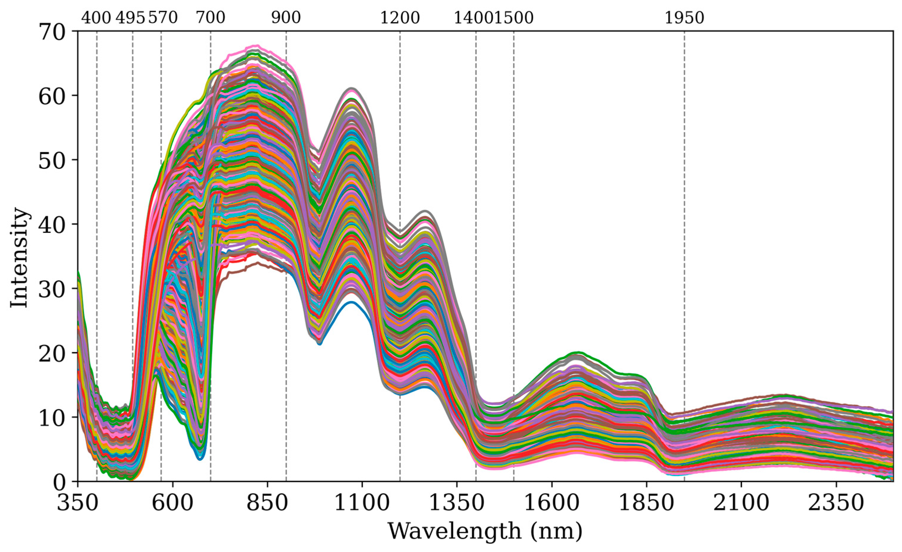
Figure 2 presents the average reflectance curves of the collected spectral data for all pesticides and their respective concentration gradients, spanning wavelengths from 350 nm to 2500 nm. This range spans both the visible and near-infrared regions. Overall, the average reflectance trends across the different pesticides and concentration gradients appear to be similar.

In the ultraviolet range (350–400 nm), high reflectance in the kumquat peel is attributed to flavonoids and other UV-absorbing compounds that protect the plant from ultraviolet radiation, enhancing its survival [28].

In the visible spectrum, the 400–495 nm band shows reduced reflectance due to absorption by pigments such as anthocyanins and carotenoids, which regulate light absorption and influence physiological functions. The 495–570 nm band exhibits higher reflectance, correlating with the peel’s yellow-orange color due to the reflection of green light. Between 570 and 700 nm, reflectance varies with chlorophyll and carotenoid content; chlorophyll absorbs blue and red light, reducing reflectance, whereas increased carotenoid levels enhance the reflection of red and yellow light [29,30,31].

In the near-infrared spectrum, the 700–1100 nm band displays reflectance fluctuations related to water and sugar content in the fruit, with decreased reflectance influenced by lower chlorophyll content and the red edge effect [32]. From 1100 to 1500 nm, the absorption characteristics of cellulose, hemicellulose, starch, and water are evident, with notable absorption valleys near 1200 nm and 1400 nm linked to the fruit’s texture, maturity, and moisture content [33,34]. The 1500–2500 nm band is critical for analyzing internal chemical components such as sugars, fatty acids, and moisture, with absorption valleys primarily due to water from 900 to 1950 nm. Beyond 1950 nm, reflectance stabilizes, indicating the saturation of absorbing substances or diminished absorption effects [35].

3.2.2. Spectral Absorption Characteristics

As shown in Figure 3, prochloraz, difenoconazole, and cypermethrin all contain aromatic rings and conjugated double bonds. In the ultraviolet–visible region (350–700 nm), their spectral absorption is primarily governed by the aromatic and conjugated systems within their molecular structures. Specifically, the presence of aromatic rings and conjugated double bonds facilitates π→π* and n→π* electronic transitions, resulting in distinct absorption peaks in the 350–450 nm range. In the 500–700 nm region, minor absorption variations may arise due to differences in molecular scattering properties. In the near-infrared region (700–2500 nm), spectral features are predominantly attributed to the vibrational and overtone absorptions of functional groups such as C-H, N-H, O-H, and C=O. [36,37,38].

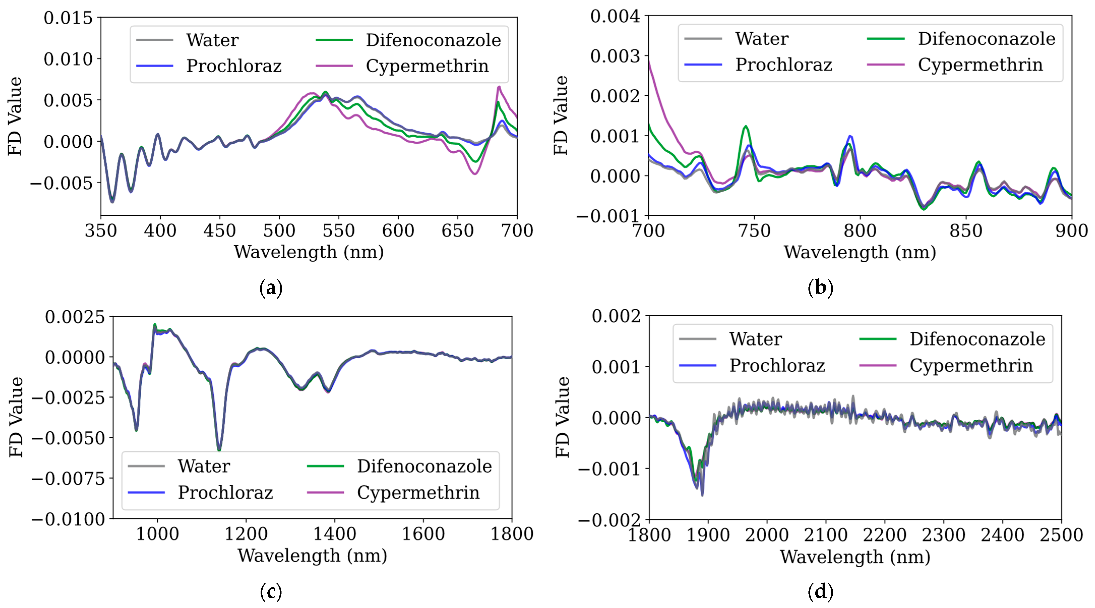
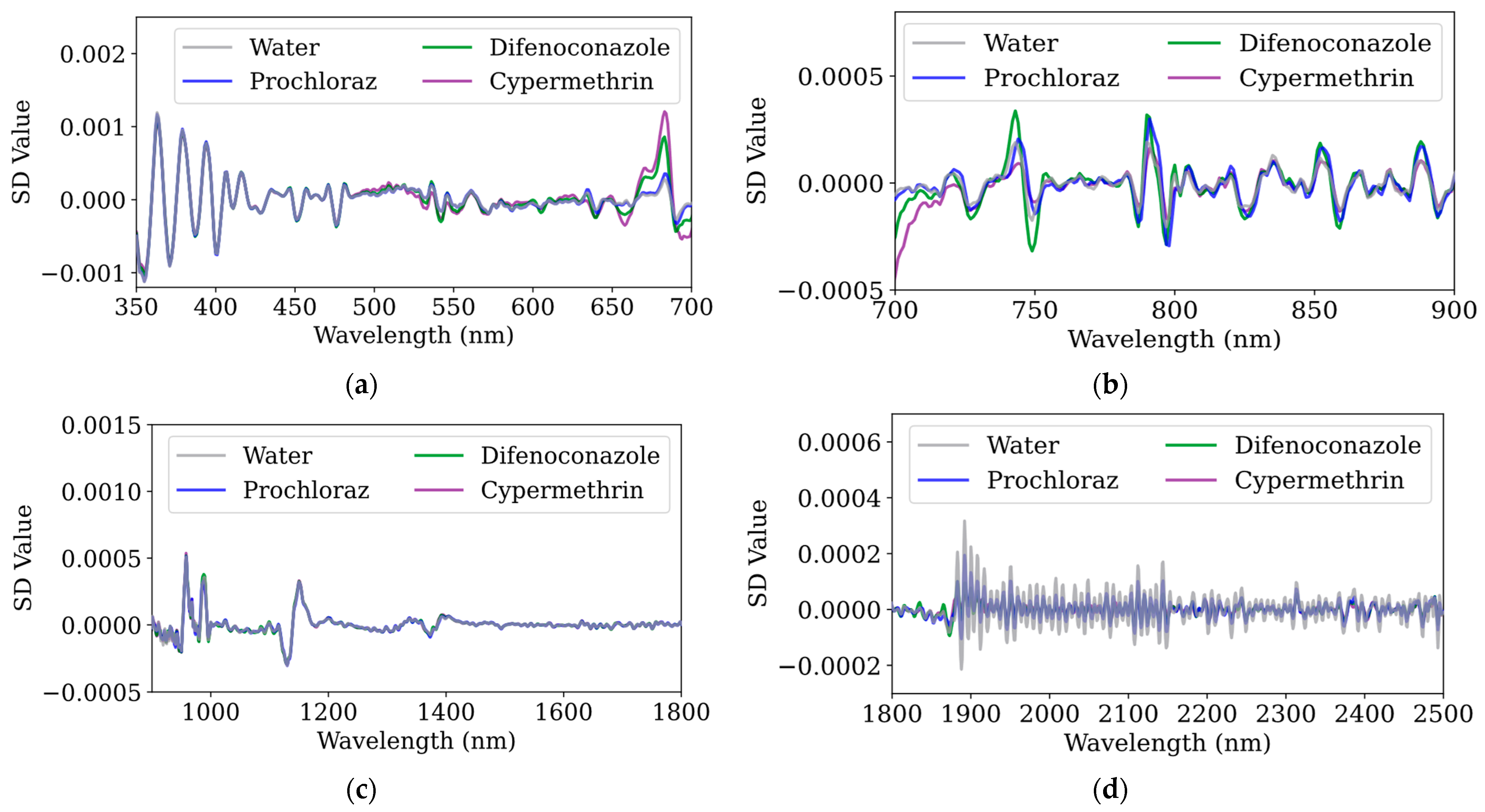
To further investigate the spectral characteristics of pesticides, this study applied first-order and second-order derivative analyses to the raw spectral data. Figure 4 and Figure 5 illustrate the first derivative and second derivative spectra of water and three pesticides (prochloraz, difenoconazole, and cypermethrin) in the 350–700 nm range. Compared to the raw spectra, derivative processing enhances subtle spectral differences: the first-order derivative highlights slope variations, facilitating the identification of upward and downward trends, while the second-order derivative further accentuates inflection points and peak–valley features, making it more sensitive to weak absorption bands and baseline variations.

As shown in Figure 4a and Figure 5a, the molecular structures of prochloraz, difenoconazole, and cypermethrin contain aromatic rings and conjugated double bonds, which induce π→π* transitions in the UV region (200–400 nm) and result in distinct absorption peaks [39,40,41]. These electronic transitions cause pronounced changes in the first-order derivative spectra—particularly between 350 and 500 nm—while the second-order derivative spectra exhibit significant fluctuations in the 350–400 nm range, reflecting strong UV absorption. In the visible region (400–700 nm), the absorption is relatively weak, though minor absorption bands lead to modest variations in both first and second derivative values. Notably, in the 550–700 nm range, the spectral features on kumquat surfaces differ markedly; the absorption peak near 550 nm is typically associated with chlorophyll b, certain carotenoids, and orange peel flavonoids, while the absorption valley at 660 nm corresponds to the low-absorption region between the two main peaks of chlorophyll a (430–450 nm and 640–680 nm). Furthermore, the strong absorption peak at 680 nm represents one of the primary absorption points of chlorophyll a, which is critical for photosynthesis [42,43].

In the 700–900 nm range, several small absorption peaks and troughs can be observed, likely related to localized water absorption, post-peak chlorophyll, other biological pigments (such as flavonoids and vitamins), and interactions between molecules and internal plant structures [44]. The first and second overtone absorptions of the C-H, N-H, and O-H bonds, associated with molecular vibrations, manifest as multiple small peaks or troughs in this band [45], as shown in Figure 4b and Figure 5b, with difenoconazole and prochloraz exhibiting significantly different absorption characteristics compared to the other two classes.

In the 900–1500 nm range, as shown in Figure 4c and Figure 5c, the pesticide and water absorption peaks significantly influence each other, showing distinct spectral responses. The first-order derivative spectra exhibit clear absorption peaks and troughs at 950 nm, 1000 nm, 1140 nm, 1225 nm, 1275 nm, 1360 nm, and 1380 nm, indicating the vibrational modes of key chemical bonds such as C-H, O-H, and N-H and water molecule characteristics [46,47]. The second-order derivative further reveals subtle peaks and troughs, where the peaks and troughs for prochloraz and difenoconazole distinctly differ from other categories. In the 1500–1800 nm range, subtle absorption peaks and troughs are primarily associated with higher-order overtones, combination frequencies, and the complexity of sample components, revealing the vibrational modes of chemical bonds and their interactions [48].

As shown in Figure 4d and Figure 5d, the first-order derivative absorption trough at 1875 nm, significantly characterized by difenoconazole, relates to its conjugated system, as well as C-H and N-H bond vibrations, water molecule interactions, and compound absorption effects [49]; when combined with the second-order derivative, water samples in the 1875–2500 nm range show more pronounced fluctuations than other categories, especially near 1900 nm, where the O-H bonds in water molecules exhibit significant absorption characteristics in this band, while organic compounds’ C-H and N-H bond absorptions are relatively lower in intensity and narrower in bandwidth [50].

3.3. Feature Visualization

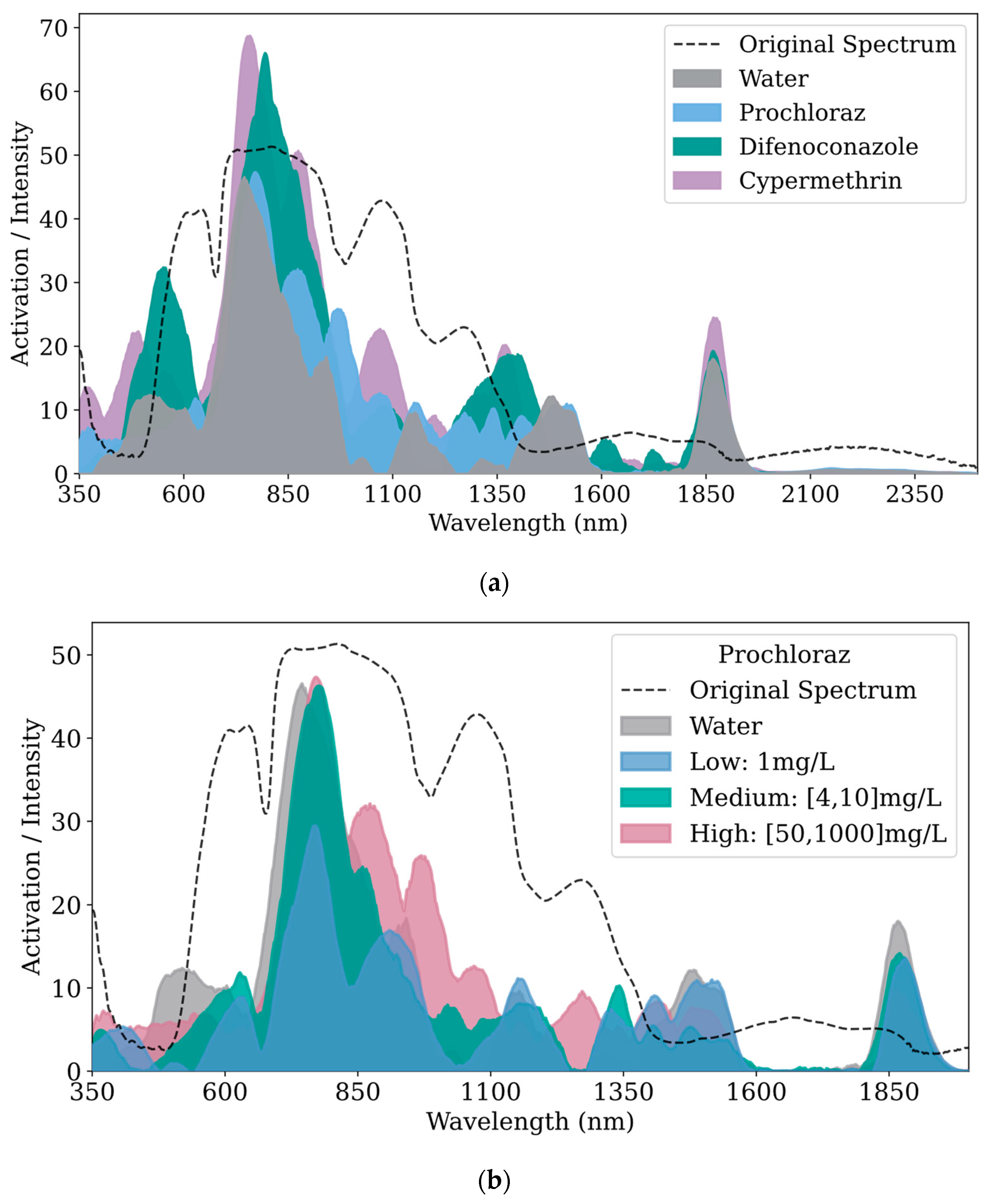
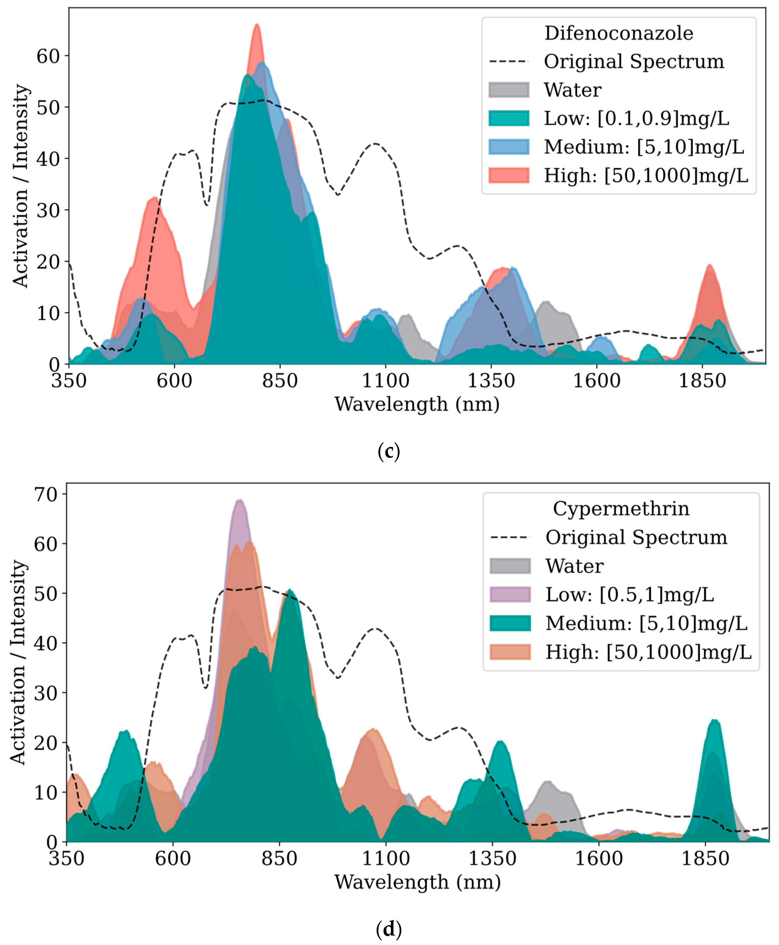
Figure 6 displays the feature visualization results extracted from the convolutional layers of the 1D-ResNet model, where the x-axis represents wavelength (nm) and the y-axis represents the intensity of spectral feature activations. Figure 6a compares the feature visualizations of three pesticides and the water control group. Figure 6b–d displays the feature visualizations comparing high, medium, and low concentrations of prochloraz, difenoconazole, and cypermethrin, respectively, against the water control group. Each subplot in Figure 6 includes the average reflectance of kumquat surfaces without residues as a reference.

In Figure 6a, clear distinctions in features across categories are observed, especially around 500 nm, 800 nm, 1050 nm, 1375 nm, and 1850 nm. The features of cypermethrin and difenoconazole are more pronounced across the entire wavelength range, particularly near 800 nm, where the feature peaks exceed those of the other categories. In the 350–650 nm band, the features of cypermethrin and difenoconazole are more distinct than those of other categories, with the highest peak for difenoconazole occurring near 550 nm. Within the 650–1250 nm band, all categories show high activation values with multiple feature peaks; the highest peaks occur near 800 nm, followed by a gradual decline. Prochloraz at 975 nm and cypermethrin near 1075 nm show distinct feature differentiation from other categories; the water group exhibits a distinct peak near 1050 nm. From 1250to 1550 nm, the feature contrasts among categories are evident, with cypermethrin and difenoconazole both displaying characteristic peaks near 1375 nm with similar peak values. Prochloraz shows four shoulder peaks near 1275 nm, 1335 nm, 1400 nm, and 1480 nm; the water group has weak features from 1250to 1400 nm, with a peak appearing only at 1485 nm. In the 1550–1800 nm band, aside from the weak feature peaks of difenoconazole near 1615 nm and 1725 nm, the activation values of other categories tend towards zero, contributing minimally to model decision-making. All categories exhibit significant feature peaks near 1875 nm, with cypermethrin’s features being the most prominent. From 2000 to 2500 nm, the activation values of all categories tend towards zero, indicating minimal contribution to model decisions; hence, this band is not displayed in subsequent subfigures and analyses.

To facilitate the observation of changes across different concentration gradients of each pesticide, the gradients were categorized into high, medium, and low, as specified in

Table 4. Classification of pesticide concentration gradients.

Type	Low (mg/L)	Median (mg/L)	High (mg/L)
Prochloraz	1	4, 7, 10	50, 100, 500, 1000
Difenoconazole	0.1, 0.3, 0.6, 0.9	5, 10	50, 100, 500, 1000
Cypermethrin	0.5, 1	5, 10	50, 100, 500, 1000

.

Figure 6b displays the feature visualization results for high, medium, and low concentrations of prochloraz. It can be observed that the activation values in the 1600–1800 nm band tend towards zero, indicating minimal contribution to the model’s decision-making process in this band. In other bands, the differences in features across prochloraz concentrations are pronounced, except for the lower concentration, which shows slightly higher peaks near 1050 nm, 1400 nm, and 1500 nm compared to medium and high concentrations. Generally, the peak values of prochloraz features decrease with decreasing concentration.

Figure 6c shows the feature visualization results for difenoconazole. Overall, the feature peaks decrease as the concentration lowers. The distinction in features between high concentration and medium/low concentrations is most apparent near 550 nm; at 1375 nm, the differences between high/medium and low concentrations are most distinct; near 1865 nm, the difference between high concentration and medium/low concentrations is also clearly visible.

Figure 6d presents the feature visualization results for cypermethrin. In the 1500–1800 nm band, the activation values tend towards zero, suggesting that the features within this band are similar and contribute minimally to the model’s decision-making. Overall, the feature peaks of cypermethrin decrease with decreasing concentration. Notably, near 750 nm, the feature peaks are highest for the low concentration, followed by the high concentration, which may be caused by instrumental errors, environmental differences, sample variability, or the chemical characteristics of the pesticide, necessitating further analysis.

Overall, the extracted features from the convolutional layers, whether differences between pesticides or among concentrations within a pesticide are pronounced in the model, contribute to an overall accuracy of 0.97. However, further model adjustments might be necessary for data with slightly lower metrics.

4. Conclusions

This study introduced a novel approach integrating handheld spectroscopy and deep learning, achieving 97% accuracy in detecting pesticide residues on kumquat surfaces. This method enables the rapid, field-based, and non-destructive detection of various pesticides and their concentration gradients by directly inputting standardized spectral data into the 1D-ResNet model, simplifying feature extraction and improving both efficiency and applicability.

Experimental results confirm the approach’s reliability and effectiveness, with a macro average of 0.96 indicating balanced performance across categories, and a weighted average of 0.97 reflecting strong performance in categories with larger sample sizes. While accuracy is slightly lower for detecting 1 mg/L prochloraz and 50 mg/L difenoconazole, the model excels in other pesticides and concentrations, with precision, recall, and F1-scores approaching or exceeding 1.00. Additionally, feature extraction and visualization from the convolutional layers of the 1D-ResNet model have provided valuable insights into its decision-making process, enhancing model interpretability and serving as a foundation for future quantitative analysis of pesticide residues.

Future work will focus on improving the model’s generalization for low-concentration pesticide detection, particularly for 1 mg/L prochloraz and 50 mg/L difenoconazole, by expanding the training dataset, applying advanced data augmentation, and fine-tuning the model. We also plan to develop a real-time system that reads data from the handheld spectrometer and automatically processes the data for immediate detection results, streamlining data flow and enabling rapid, precise detection. Furthermore, a class-incremental learning strategy will be implemented to introduce new pesticide residue categories while retaining the model’s ability to differentiate older ones, enhancing its flexibility and long-term applicability. These advancements will improve detection efficiency and provide better support for the safety monitoring of specialty crops like kumquats.