Computational Fluid Dynamics Simulation and Quantification of Solar Greenhouse Temperature Based on Real Canopy Structure

Abstract

The temperature distribution of the cucumber canopy in an energy-saving solar greenhouse was simulated in this study. The canopy temperature data of autumn and winter cucumber were collected using temperature sensors, and the spatial heterogeneity of temperature distribution was analyzed. Utilizing ground-based LiDAR scanning, point cloud data of plant canopies were acquired to construct a convex hull porous model and leaf organ model. Validation against real solar greenhouse measurements revealed the convex hull porous model’s superior performance over the hexahedral porous model in computational fluid dynamics (CFD) simulations, with a root mean square error of 0.71 °C and a mean relative error of 2.9%, as opposed to 0.99 °C and 4.3%, respectively. Simulations in a scaled virtual greenhouse demonstrated the convex hull porous model and leaf organ model reduced temperature variation by 0.6 °C and 2.3 °C compared to the hexahedral porous model. The leaf organ model particularly provided a smooth temperature transition among leaves, closely approximating actual crop conditions. These results offer insights for crop model selection in greenhouse CFD modeling.

1. Introduction

Solar greenhouses are highly energy-efficient horticultural facilities that can effectively solve the problem of year-round vegetable supply in the cold regions of northern China. Cucumber has the largest greenhouse cultivation area in China, with an average annual sowing area of about 1.23 million hectares and an annual total yield of about 66.23 million tons. Its yield is ranked first globally among all crops and shows an increasing annual trend [1]. The growth and yield of cucumbers are closely influenced by various microclimatic factors, including greenhouse internal temperature, light intensity, and relative humidity [2]. Due to its unique structural properties, the climate and environmental conditions are not evenly distributed in solar greenhouses. This unevenness results in significant heterogeneity in the cucumber canopy structure. Empirical studies have demonstrated that the optimization of the indoor thermal environment within solar greenhouses can significantly enhance the physiological performance and yield of cucumber plants, which has specifically led to increases of 30% in plant height, 25% in stem diameter, and 28% in fruit yield, respectively [3]. Therefore, quantifying the spatiotemporal distribution and variations of environmental parameters is crucial for creating optimal conditions for cucumber growth and promoting sustainable agricultural development.

Previous studies have established a thermal balance physical model of a solar greenhouse using data collected from experiments with the principle of mass-energy transfer. This model can reflect the energy exchange relationship between the solar greenhouse enclosure structure and the external weather environment [4,5]. However, it requires on-site experimental research that is costly and model results are often limited by experimental conditions [6]. Further, this model assumes a steady-state uniform energy distribution that does not reflect the actual production situation [7]. Research on microclimate simulation models that include the environmental characteristics of solar greenhouses has increased significantly. Computational Fluid Dynamics (CFD), which is based on the principle of greenhouse thermal balance, enables the development of dynamic models for microclimates such as temperature and light. It can simulate and analyze the spatial distribution characteristics of microclimates within the greenhouse [8]. This approach aids researchers in optimizing systems such as ventilation and temperature control, ultimately enhancing crop growth quality and yield in greenhouses [9,10]. Saberian and Sajadiye [11] used a variable solar radiation model to develop a three-dimensional CFD model of dynamic solar heat load and temperature field in a solar greenhouse, leading to an enhanced ability to monitor and analyze the dynamic microclimate heterogeneity in the vertical direction from the roof to the ground. Liu et al. [12] developed a CFD coupling model integrating crop canopy and external weather. This model accurately simulated the spatiotemporal distribution of three-dimensional canopy condensation of greenhouse cucumbers at night, providing valuable insights for early warning and control strategies.

While significant progress has been made in studying temperature distribution in solar greenhouses, most CFD-based greenhouse modeling studies focus on empty greenhouses or treat crops as uniform porous media. This approach tends to ignore or simplify the microclimate differences caused by the spatial heterogeneity of crop canopies [13,14,15]. The three-dimensional structure of crops directly affects their light interception capacity and is also the most important feature for determining plant phenotypes. Crop life processes, including temperature regulation, transpiration, and carbon dioxide flux, significantly impact their surrounding environment. Accounting for the dynamic and distributed energy exchange between the crop canopy and the greenhouse environment can significantly improve the accuracy of the greenhouse microclimate CFD model [16]. Consequently, the meticulous consideration of the dynamic energy interchange between the crop canopy and the greenhouse ambiance is of paramount importance for augmenting the precision of CFD models pertaining to the microclimate within greenhouses.

In recent years, advancement in 3D reconstruction technology for crop canopies has significantly progressed, leading to improved and diversified methods for data collection methods and enhanced efficiency. Based on differences in sampling and reconstruction methods, two common approaches for crop 3D reconstruction have emerged: 3D reconstruction based on image sequences [17], and 3D reconstruction using lidar scanning [18,19]. The 3D reconstruction technology based on image sequences is good for reconstructing individual crops, but it has limitations when applied to the 3D reconstruction of group crops in greenhouses. Lidar technology effectively solves this problem. By calculating the time difference between emitted and returned pulses, LiDAR determines the position of the target object. The resulting data is in the form of a point cloud, which contains the spatial point coordinates, intensity, and RGB information of the target object [20]. The use of ground-based lidar for high-precision point cloud data collection can accurately obtain information such as crop position, height, aboveground biomass, canopy coverage, leaf area index, etc. Researchers have applied high-precision LiDAR to the phenotyping of crops such as tomatoes, rice, and corn [21,22,23]. Currently, LiDAR technology has been used in various areas such as monitoring crop stress response, estimating crop economic yield, and calculating light interception [24,25,26,27].

The integration of high-precision and efficient methodologies for acquiring the three-dimensional architecture of plants with CFD has facilitated a more profound comprehension of the underlying mechanisms and dynamic processes associated with crop growth. This approach is of paramount importance in propelling research endeavors related to high-throughput plant phenotyping and the synergistic analysis of plant functionality and structural characteristics. Yu et al. [28] utilized CFD simulation to assess the thermal performance of a 3D tomato model constructed with SolidWorks. The simulation results were consistent with the measurements taken at the same height within a greenhouse, with a standard deviation of only 0.069 K between the calculated and measured data. This finding underscores the reliability of the computational model and its potential applications. Gu et al. [29] conducted 3D modeling of the soybean canopy using a scanner, and the results indicated that the CFD simulation had a mean absolute error of 0.4 °C in leaf temperature. These outcomes confirm the consistency between the 3D model and traditional porous medium models. The application of three-dimensional plant structures obtained from LiDAR scanning in greenhouse CFD simulations has not been widely explored, which is the experimental method we will investigate in this paper.

The overall goal of this paper is to simulate the thermal environment of the solar greenhouse canopy using CFD technology. By comparing and analyzing the collected test data from the solar greenhouse, the temperature distribution patterns of the canopy are examined. Additionally, LiDAR-based crop canopy point cloud data are used for three-dimensional modeling. CFD is then used to analyze the differences between the conventional porous media model and the greenhouse thermal environment simulation using the real three-dimensional canopy structure model, offering insights for the simulation and analysis of the three-dimensional crop leaf level in the solar greenhouse field using CFD technology.

2. Materials and Methods

2.1. Experimental Design

The experiment was conducted from 21 September to 10 December 2023. Temperature sensors (RC-4, Elitech, Xuzhou, China) were used to continuously monitor the surface temperature changes of each enclosure structure (front roof, rear roof, rear wall, soil) inside the solar greenhouse. Each sensor probe was treated to prevent light radiation interference. The greenhouse was divided into test areas every 20 m in the east-west direction. Using the northeast corner of the greenhouse as the origin, area A extends 20 m from west to east, area B spans from 20 m to 40 m, and area C covers from 40 m to 60 m in length. In each planting test area, a total of 27 temperature sensors were arranged, with 9 sensors placed in a 3 × 3 grid pattern. These sensors were positioned at horizontal intervals of 2.0 m and at vertical heights of 0.5 m, 1.0 m, and 1.5 m above the ground. The layout of the sensors is shown in Figure 1. These sensors recorded data at the same frequency as the outdoor meteorological station, collecting data every 10 min.

To explore the possible heterogeneity of canopy temperature at different developmental stages, three typical sunny days were selected for analysis: the seedling stage, the initial flowering stage, and the fruiting stage of cucumber crops. The seedling stage was observed on 30 September 2023, with an average canopy height of 0.55 m. The initial flowering stage was observed on 14 October 2023, with an average canopy height of 1.17 m. The fruiting stage was taken on 2 November 2023, with an average canopy height of 1.79 m. Due to the variation in canopy height at different developmental stages, only the horizontal plane at a height of 0.5 m can be used to describe the canopy temperature during the seedling stage. During the initial flowering stage, the horizontal planes at both 0.5 m and 1.0 m can be used to study canopy temperature. During the fruiting stage, temperatures at all three horizontal plane heights (0.5 m, 1.0 m, and 1.5 m) are suitable for analyzing canopy temperature.

During the cucumber fruiting stage, the cucumber canopy was scanned using a ground-based LiDAR FARO SCAN (FARO Focus, Lake Mary, FL, USA). In the course of the scanning procedure, the system adheres to the predefined settings, which include a 1/4 resolution scale, a quality enhancement factor of 2×, and a High Dynamic Range (HDR) multiplier of 5×. Prior to each scan, a target ball was placed between the ridges to identify the unique spatial point within the field of view of the adjacent scanning station. For data collection, a six-stack scanning method was used with LiDARplaced at the four corners and the midpoint of the long side of the collection area. Each scan took about 10 min. The collected ground-based LiDAR data was processed using the supporting software FARO SCENE 2023. This software was used to align and fuse the multi-stack three-dimensional point cloud, followed by steps to remove the ground, perform denoising, and extract the green plant point cloud. For more specific procedural details, reference should be made to the study conducted by Wang et al. [30]. Finally, data containing only plant point clouds (Figure 2a), single plant point cloud data (Figure 2b), and single plant three-dimensional convex hulls (Figure 2c) and leaf organ models (Figure 2d) constructed based on this are obtained.

2.2. Basic Control Equations

2.2.1. Energy Balance Equations

The heat transfer and fluid flow inside the greenhouse follow the laws of physical conservation. The flow of gas in a solar greenhouse follows turbulent motion, and the Standard $k-\epsilon$ model is used for numerical simulation calculations. The control equations include the continuity equation (mass conservation), the momentum conservation equation, the $k$ (turbulent kinetic energy) equation, and the $\epsilon$ (dissipation rate) equation, all of which can be written in the following general form [31,32,33]:

$${\displaystyle \frac{\partial \left(\rho \varphi \right)}{\partial t}}+div\left(\rho \overrightarrow{V}\varphi \right)=div\left({\mathsf{\Gamma }}_{\varphi }grad\varphi \right)+S_{\varphi }$$

(1)

where $\varphi$ is a universal physical variable, representing the solution variables such as mass, velocity, and temperature, $\rho$ is the fluid density (kg m⁻³), $\overrightarrow{V}$ represents the velocity vector (m s⁻¹), ${\Gamma }_{\varphi }$ is the generalized diffusion coefficient of the variable $\varphi$, $S_{\varphi }$ is the generalized source term of the variable $\varphi$, and $div$ and $grad$ are the divergence and gradient operators, respectively.

2.2.2. Radiation Model

Solar radiation plays an important role in the microclimate of a solar greenhouse. During daylight, solar irradiance traverses the translucent facade of the greenhouse, interacting with the surfaces of the diverse enclosure structures via radiative heat exchange processes. Nocturnal conditions witness the cessation of solar irradiance and the subsequent closure of the insulating cover, which results in the enclosure structures maintaining a relatively elevated inner surface temperature. This temperature disparity significantly contributes to the radiative heat exchange, thereby exerting a substantial influence on the thermal distribution within the greenhouse. Consequently, the present investigation employs the Discrete Ordinates Radiation Model (DO model) to conduct computational analyses [34]. The model integrates temporal and spatial variables, including the local time, geographic coordinates, and meteorological parameters specific to Beijing, utilizing a ray-tracing approach to simulate the radiative heat transfer dynamics. Thus, the real-time simulation of the solar altitude angle and the angle of incidence is achieved. The specific formula is as follows:

$$\nabla \left(I_{\lambda }\left(\overrightarrow{r},\overrightarrow{s}\right)\overrightarrow{s}\right)+\left(a_{\lambda }+{\sigma }_s\right)I_{\lambda }\left(\overrightarrow{r},\overrightarrow{s}\right)=a_{\lambda }{n}_{\lambda }^2{\displaystyle \frac{\sigma T^4}{\pi }}+{\displaystyle \frac{{\sigma }_s}{4\pi }}\times {\int }_0^{4\pi }{I}_{\lambda }\left(\overrightarrow{r},\overrightarrow{s^{\prime }}\right)\varphi \left(\overrightarrow{\mathrm{s}},\overrightarrow{{\mathrm{s}}^{\prime }}\right)\mathrm{d}\Omega$$

(2)

where $I_{\lambda }$ is the radiation intensity (W m⁻²), $\overrightarrow{r}$ is the position vector (m), $\overrightarrow{s}$ is the direction vector, $\nabla$ is the divergence operator, $\overrightarrow{s^{\prime }}$ is the scattering direction vector, $a_{\lambda }$ is the absorption coefficient (m⁻¹), $\sigma$ is the Stefan Boltzmann constant (5.67 × 10⁻⁸ Wm⁻² K⁻⁴), ${\sigma }_s$ is the scattering coefficient (m⁻¹), $n_{\lambda }$ is the refractive index, $T$ is the temperature (°C), $\varphi$ is the phase function, and $\Omega$ is the radiation solid angle.

The capacity of the atmosphere to absorb solar radiation may be characterized by the effective sky temperature. Under clear and cloudless weather conditions, the effective sky temperature is given by [35]:

$$T_{\mathrm{sky}}=0.055\times 2T_0^{1.5}$$

(3)

where $T_0$ is the outdoor air temperature (K).

2.2.3. Plant Porous Media Model

Porous media is a mixture of solid skeletons and fluid in the skeleton gaps. This study uses the plant porous media model to simulate the influence of plants. The drag effect of plants on air is reflected by the source term of the momentum equation of the basic equation. Assuming that the plant is a uniform isotropic porous medium, there is:

$$S_{\varphi }=-\left({\displaystyle \frac{\mu }{a}}\nu +Y\rho \left|\nu \right|{\displaystyle \frac{\nu }{2}}\right)$$

(4)

where $S_{\varphi }$ is the momentum source term, $\mathsf{\mu }$ is the dynamic viscosity of air (N·s·m⁻²), and $a$ is the porosity of the medium obtained through experimental measurement. $Y$ is the nonlinear momentum dissipation coefficient (m⁻¹), $\rho$ is the air density (kg m⁻³), and $\nu$ is the airflow velocity (m s⁻¹).

The corresponding expression for the plant drag effect in terms of momentum source per unit volume of the canopy can be written as [36]:

$$S_{\varphi }=-\rho C_D{\nu }^{2}LAD$$

(5)

where $LAD$ is the Leaf Area Density (m²/m³), and $C_D$ is the drag coefficient, with an experimental value of 0.32 [37].

2.3. Model Establishment

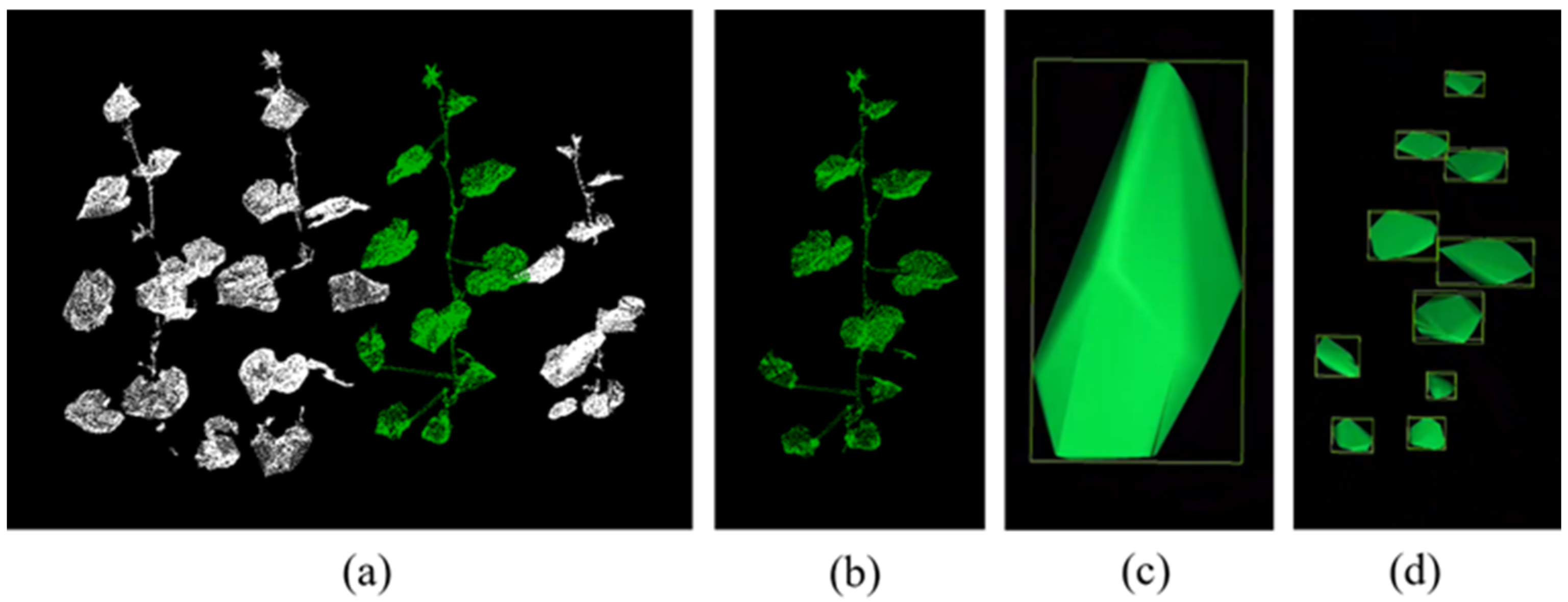
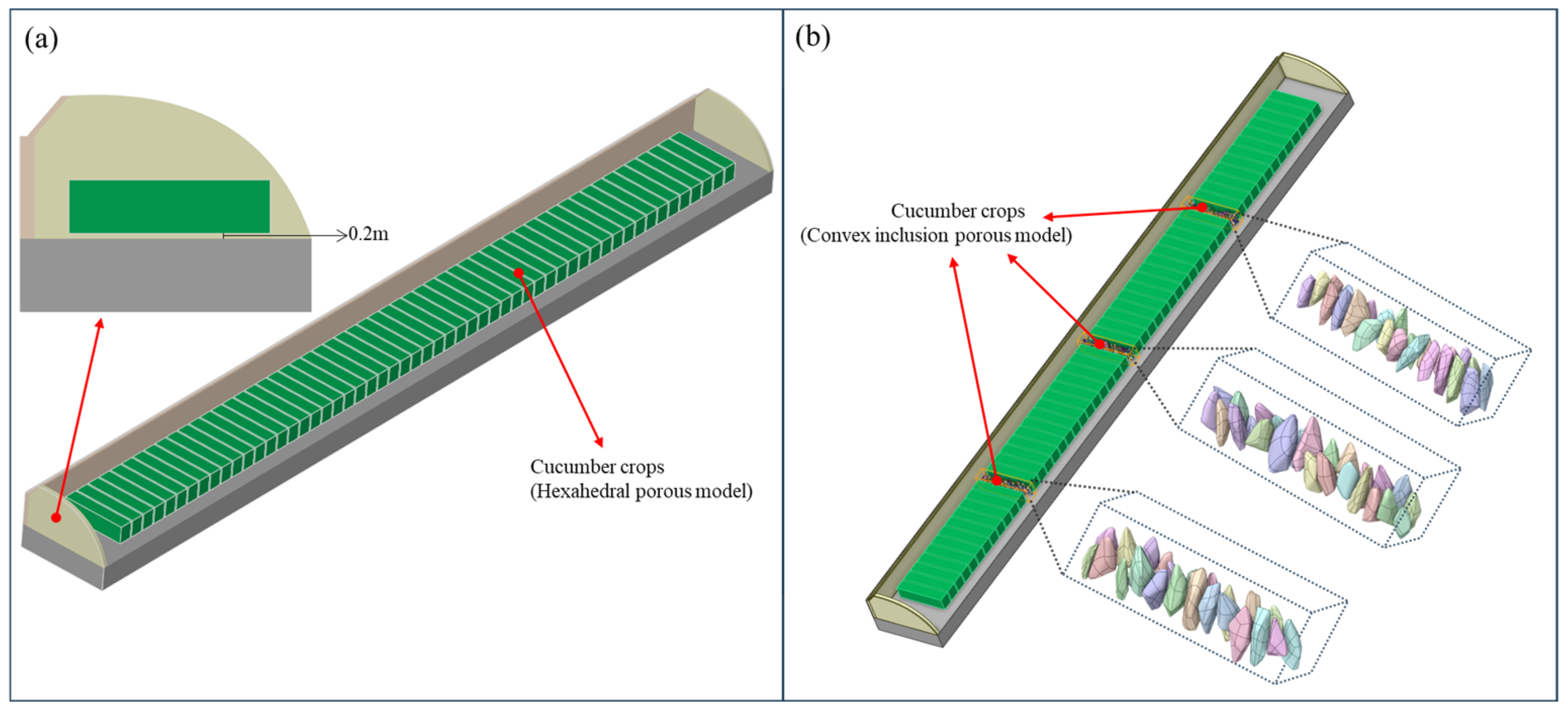
2.3.1. Real Greenhouse 3D Structural Model and Simplified Plant Model Assumptions

Based on the actual dimension of the test greenhouse, a three-dimensional solid model was established in Ansys 2023 R2 SpaceClaim. In this model, the positive direction of the x-axis represents the south, the positive direction of the y-axis represents the west, and the positive direction of the z-axis is vertically upwards. To simplify the complex heat transfer process within the greenhouse while maintaining accuracy, the following assumptions were made for the heat transfer model: (1) The air inside the greenhouse is treated as a viscous, incompressible ideal gas in a turbulent state; (2) It is assumed that there is no ventilation in the greenhouse during the simulation process; (3) The influence of arches and ducts on the heat transfer is ignored; (4) The growth conditions of each plant in the greenhouse are assumed to be uniform, and each plant is treated as an equivalent porous medium model [16]; (5) The buoyancy term caused by temperature differences satisfies the Boussinesq assumption.

Given the large size of the actual greenhouse, which measures 80 m in length and 8 m in span with 55 rows of cucumber plants, modeling the fine canopy structure of all plants would require huge amount of data and need substantial computational resources that are well beyond the capacity of the software. To address this challenge, a simplification approach was adapted. For the hexahedral porous model, each row of crops is represented as a hexahedron with dimensions of 1.2 m × 1.8 m × 5.8 m, resulting in 55 rows of simplified hexahedral crop areas in this greenhouse (Figure 3a). For the convex hull porous model, the three rows of hexahedral porous models located at 20 m, 40 m, and 60 m were replaced by the convex hull porous models generated from point clouds (Figure 3b). Since the root and stem parts of the cucumber crop close to the ground are relatively sparse and have large porosity, the height below 0.2 m from the ground is set as blank during modeling.

2.3.2. Small Greenhouse Model Considering the Fine 3D Structure of Plants

To further explore the microclimate distribution in the greenhouse while considering the fine 3D structure of crops, a small artificial climate chamber greenhouse was virtually designed. The greenhouse has dimensions of 2.0 m × 2.0 m × 2.0 m, with a 30 cm high sunshade installed on the top of the greenhouse. The entire greenhouse is modeled as a fully enclosed environment. Four cucumber plants of different heights, measured by ground-based lidar, were selected. Three different models of hexahedral porous medium, convex hull porous medium, and single leaf assembly were used to simulate and calculate each cucumber (Figure 4). In the Fluent software configuration, the convex hull model is designated as a porous medium, employing an identical $C_D$ value to that of the hexahedral porous model. The volume of each model can be directly measured within the SpaceClaim 2023 software. Convex hull models exhibit higher LAD values than porous hexahedral models, given their smaller volumes and constant leaf area. The leaf organ model, conversely, does not treat the leaves as a porous medium; rather, each leaf organ of the cucumber is a solid option within the software, with all leaves being endowed with uniform thermodynamic and radiative characteristics.

2.3.3. Grid Generation and Independence Verification

In this study, an unstructured grid system is used. The grid is locally refined based on the temperature field’s gradient distribution within the calculation area. For the large greenhouse with the same area as the actual dimension in this study, grid systems with grid numbers 1,124,329, 1,491,983, and 1,896,258 are selected to verify the grid independence of the hexahedral porous medium plant model; grid systems with grid numbers 2,858,121, 10,336,415, and 31,898,827 are selected to verify the grid independence of the convex hull porous plant model. For the small greenhouse, grid systems with grid numbers 53,676, 96,911, and 128,674 were selected to verify the grid independence of the greenhouse using the hexahedral porous medium crop model; grid systems with grid numbers 784,465, 922,643, and 1,377,306 were selected to verify the grid independence of the greenhouse using the convex hull plant model generated by point cloud; grid systems with grid numbers of 1,058,893, 1,544,039 and 2,021,265 were selected to verify the grid independence of the greenhouse using the leaf organ model generated by point cloud. By testing these various grid systems, the study ensures that the simulation results are independent of grid resolution.

2.4. Boundary Conditions

Boundary conditions are crucial to the quality and accuracy of the numerical results. This study used Ansys 2023 R2 Fluent software to set boundary conditions in the software based on experimental test data. The absorptivity and transmittance of the greenhouse film for visible light and near-infrared light were set in the radiation model to simulate its selectivity for different wavelengths. From 08:00 to 18:00, the south-facing roof is defined as a layer of transparent plastic film, while for the rest of the time, it is set as a layer of Heat preservation quilt. During the day, the short-wavelength transmittance of the plastic film on the south side of the greenhouse, along with all other envelope structures, is set to 0.8. Since the plastic film is almost impermeable to infrared radiation, a very large absorption coefficient is applied to the long-wavelength portion. The east and west walls of the greenhouse are constructed with opaque materials, which cast shadows during specific times of the day, particularly in the early morning and late afternoon. These shadows can influence the distribution of solar radiation within the greenhouse, affecting both temperature and light availability for plant growth. In the CFD simulations, the shading effect was incorporated by defining ray-tracing boundary conditions for solar radiation. Energy inside and outside the greenhouse is exchanged in three forms: convection, heat conduction, and radiation through the greenhouse film and walls. According to the experimental arrangement of measurement points, the measured greenhouse thermal environment parameters are used as the initial conditions and verification data for the three-dimensional transient thermal environment simulation of the solar greenhouse. The measured data of the outside of the greenhouse and the greenhouse enclosure structure at 00:00 on 2 November 2023, a typical sunny day, were selected as the initial conditions for the simulation to simulate the thermal environment of the solar greenhouse from 00:00 on the same day to 00:00 on the next day. Integrate the geographical latitude and longitude of Beijing, along with the effective sky temperature and solar irradiance intensity, derived from experimental measurements, into the Fluent CFD solver. The experimental greenhouse and the simulated greenhouse wall are modeled with coupled boundary conditions, as implemented in the Fluent software settings. The greenhouse enclosure structure and crops are affected by solar radiation, and the rest do not participate in the radiation calculation. The relevant material thermophysical properties set within the Fluent software are shown in

Table 1. Physical properties of the greenhouse materials.

Materials	Thickness (mm)	Density (kgm−3)	Specific Heat Capacity (J kg−1K−1)	Thermal Coefficient (Wm−1K−1)	Absorption Coefficient (m−1)	Scattering Coefficient (m−1)	Refractive Index
Air	-	1.225	1006	0.02	0.15	0	1.0
Brick wall	350	1700	1050	0.81	0.5	0	1.2
Polystyrene board	80	50	1300	0.03	0.3	0	1.1
Board	60	550	2500	0.29	0.3	0	1.2
Soil	-	1860	1150	1.28	0.8	1.0	1.9
Plastic film	0.1	70	2300	0.19	0.1	0.3	1.2
Heat preservation quilt	40	950	1000	0.05	0.1	0	1.2
Canopy	-	1001	3300	0.4	0.6	0.1	1.5

.

2.5. Calculation Strategy

The calculation and simulation were performed using Ansys 2023 R2 Fluent. A non-steady-state heat transfer model was used with the SIMPLE algorithm for the coupled calculation of pressure momentum and velocity momentum. The least squares method was used for the gradient term in the spatial discretization design, and the second-order upwind scheme was used for momentum, energy, and viscosity terms. The residual convergence criterion for the energy term was set to less than 10⁻⁶, while the continuity equation and the $k-\epsilon$ equation was set to less than 10⁻³. The calculation used a time stop of 60 s, with a total of 1440 steps to model 24 h temperature change.

3. Results

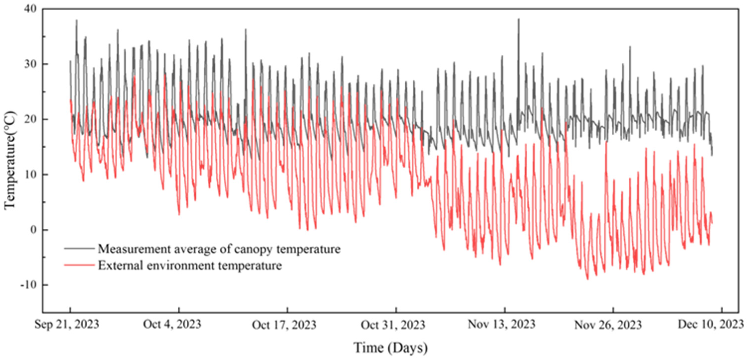
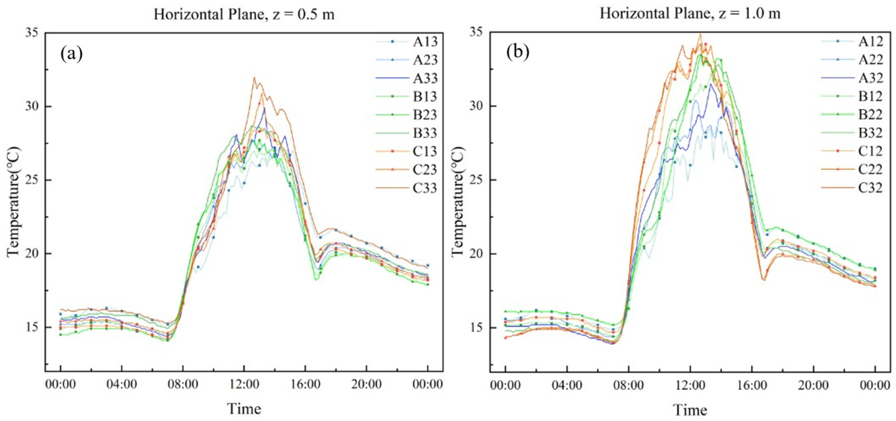
3.1. Experimental Data Analysis

Figure 5 shows the average temperature of the 27 stations in the greenhouse and 1 station outdoors from 21 September 2023 to 10 December 2023. The greenhouse has taken warming measures since October 29.

Figure 6 shows the canopy temperature at the height of 0.5 m measured on 30 September 2023. The measured temperature distribution in the north–south (x direction) across Zones A, B, and C of the greenhouse indicates a clear thermal gradient, where temperatures were consistently higher in the south compared to the north. Within 24 h, the measured value at A33 in the south of Zone A was 1.8 °C higher than at A13 in the north; the measured value at B33 in the south of Zone B was 1.4 °C higher than at B13 in the north, and the measured value at C33 in the south of Zone C was 1.4 °C higher than at C13 in the north.

In the east–west y direction, before 06:40, the average temperature was the highest on the east side (Zone A) and the lowest on the west side (Zone C). From 06:40 to 14:30, the average canopy temperature of the greenhouse in Zone C was higher than Zone A, reaching an average maximum temperature difference of 3.4 °C at 09:00. After 14:30, the average canopy temperature in Zone A gradually exceeded that of Zone C, reaching an average maximum temperature difference of 1.3 °C at 15:50.

The study on 14 October 2023 added canopy temperature data at a height of 1.0 m (Figure 7). In the north–south direction, before 08:00, the north side of areas A, B, and C had higher average temperatures than the south side. From 08:10 to 15:00, the south side of areas A, B, and C had higher temperatures than the north side. After 15:10, the north side gradually became warmer than the south side. In addition, the north–south temperature difference at 1.0 m was greater than at 05 m. The maximum north–south temperature difference reached 4.8 °C at 13:30 at the 1.0 m height, compared to 3.6 °C at 12:40 at the 0.5 m height.

In the east–west y direction, before 07:30, the average canopy temperature in area A was higher than in area C. From 07:40 to 15:50, the average canopy temperature in area C was higher than in area A, with the maximum temperature difference of 4.3 °C observed at 12:40. After 16:00, the temperature in area A gradually became higher than in area C, and the maximum temperature difference reached 0.6 °C at 16:30. The east–west temperature difference at a height of 1.0 m was more pronounced than at 0.5 m. The 1.0 m canopy reached a maximum east–west temperature difference of 6.4 °C at 10:50 while the 0.5 m canopy reached a maximum east–west temperature difference of 2.8 °C at 13:00.

In the vertical z direction, the average temperature at 0.5 m was higher than at 1.0 m at night. From 07:50, the average temperature at 1.0 m gradually exceeded that at 0.5 m. The maximum vertical temperature difference was observed at 10:50 in area A, with the average temperature at 1.0 m being 8.0 °C higher than at 0.5 m. From 15:50, the average temperature at 0.5 m began to exceed that at 1.0 m again.

The measurements at three heights on 2 November 2023 (Figure 8) can be used to study canopy temperature. In the north–south x direction, prior to 08:40, the average temperature on the north side of areas A, B, and C was higher than on the south side. However, after 08:50, the temperature on the south side of these areas gradually increased and surpassed the temperature on the north side. The time at which the temperature on the north side exceeded that on the south side varied depending on the canopy height: at 14:50 for 0.5 m, 15:30 for 1.0 m, and 16:10 for 1.5 m. The north–south temperature difference was greatest at a canopy height of 1.5 m, with the south side being 2.9 °C higher than the north side at 12:40. In contrast, the north–south temperature difference at a canopy height of 0.5 m was the smallest, staying below 1.5 °C throughout the 24 h period.

In the east–west y direction, from 11:10 to 18:30, the average canopy temperature in area C was higher than in area A, with the maximum temperature difference reaching 3.2 °C at 12:40. At other times, the average canopy temperature in area A was higher than that in area C. The east–west temperature difference was more pronounced at a canopy height of 1.5 m than at 0.5 m. At 1.5 m, the maximum east–west temperature difference was 3.6 °C at 12:30, while at 0.5 m, the maximum temperature difference was, also at 12:30.

In the vertical z direction, the average temperature at the 1.5 m and 1.0 m canopy height was higher than at 0.5 m. The temperature difference followed a pattern of first increasing and then decreasing throughout the day. At 00:00, the average vertical temperature difference between 1.5 m and 0.5 m reaches a maximum of 4.2 °C. It then gradually decreased and dropped to within 0.1 °C by 23:30.

3.2. CFD Grid Independence Verification Results

Table 2. Comparison results of grid sensitivity analysis.

	Greenhouse Models *	Total Number of Elements	Minimum Orthogonal Quality	Maximum Skewness	Average Minimum Air Temperature (°C)
Coarse grid	a	1,124,329	0.24	0.76	25.2
	b	2,858,121	0.19	0.8	24.8
	c	53,676	0.23	0.78	24.9
	d	784,465	0.23	0.77	25.5
	e	1,058,893	0.21	0.79	25.8
Middle grid	a	1,491,983	0.32	0.68	22.1
	b	10,336,415	0.27	0.73	22.5
	c	96,911	0.34	0.66	22.3
	d	922,643	0.35	0.66	22.6
	e	1,544,039	0.29	0.72	22.5
Fine grid	a	1,896,258	0.29	0.71	21.8
	b	31,898,827	0.26	0.74	22.0
	c	128,674	0.29	0.7	22.1
	d	1,377,306	0.31	0.69	22.5
	e	2,021,265	0.25	0.75	22.5

* Hexahedral porous model (a) and Convex hull porous model (b) for simulated real greenhouse; Hexahedral porous model (c), Convex hull porous model (d), and Leaf organ model (e) for simulated small virtual greenhouse.

shows the average minimum temperature of simulations using different numbers of grids in the selected grid independence verification scenarios. Compared to the coarse grid simulations, those using medium-sized grids exhibit noticeable temperature differences. However, when compared with the fine grid simulations, the maximum temperature difference using medium-sized grids is within 3%. This indicates that increasing the number of grids for the medium-sized grid simulations will hardly affect the simulation results. The medium-sized grid system can already produce accurate simulation results that are independent of grid resolution. To optimize computing resources while ensuring the simulation accuracy, this study uses medium-sized grids for the simulation analysis.

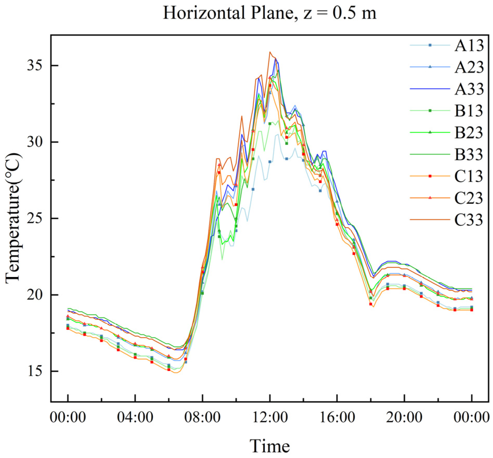
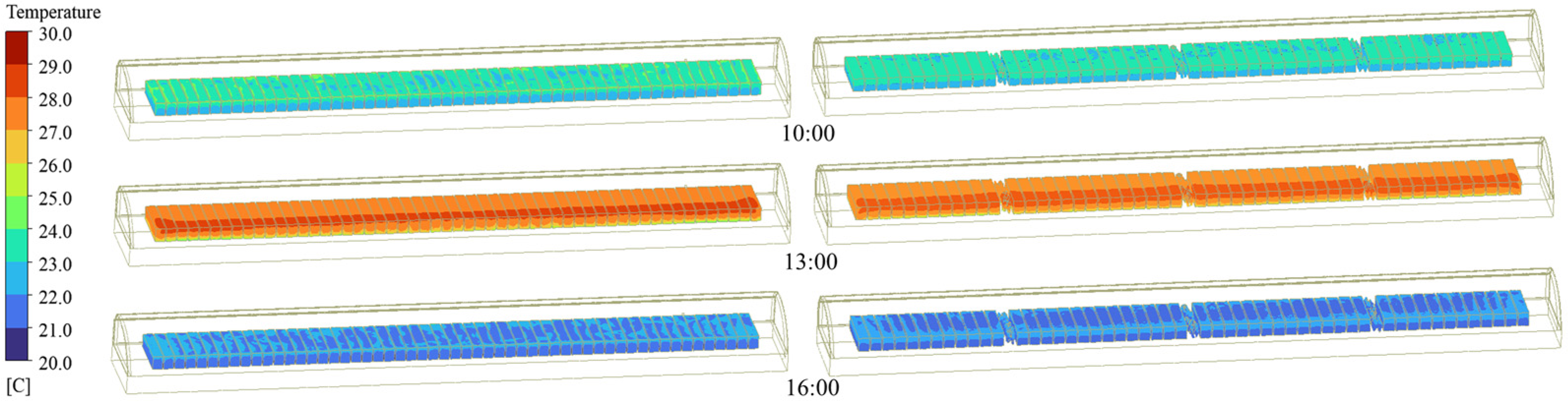
3.3. CFD Simulation Analysis of a Real Greenhouse

The typical internal and external environmental parameters of the greenhouse from 00:00 on 2 November 2023 to 00:00 on the following day were selected for analysis. The average temperature of 27 canopy measurement points was compared with the simulated average temperature from the established CFD heat transfer model. The trends of the simulated values for both models closely match that of the measured values, as shown in Figure 9. For the hexahedral porous model, the absolute error between the measured average temperature of the 27 measurement points in the greenhouse and the CFD simulated average temperature ranged from 0.1 to 1.8 °C. The root mean square error was 0.99 °C, the average relative error was 4.3%, and the maximum relative error was 7.1%. For the convex hull porous model, the absolute error ranged from 0.1 to 1.1 °C, the root mean square error was 0.71 °C, the average relative error was 2.9%, and the maximum relative error was 6.5%. Overall, the measured and simulated values of both models showed good agreement, confirming the reliability of the heat transfer model and its numerical calculation method.

The CFD simulation results established at 10:00, 13:00, and 16:00 on 2 November 2023, are depicted in Figure 10. Both the hexahedral porous model and the convex hull porous medium model demonstrated similar patterns of temperature distribution. At 10:00 and 13:00 the temperatures in regions A, B, and C were observed to be higher on the southern side compared to the northern side, with higher temperatures also noted in the upper levels compared to the lower levels. At 13:00, the southern side exhibited a significantly higher temperature than the northern side, and the temperature contour maps at the three heights of 1.5 m, 1.0 m, and 0.5 m revealed pronounced stratification. By 16:00, the temperature disparity between the north and south had diminished, and regions where the northern side surpassed the southern side in temperature had appeared. These simulation results are consistent with the findings from previous analysis.

Figure 11 illustrates the temperature differences between the actual measured canopy temperatures at 27 specific points within the experimental greenhouse and the simulated values generated by the heat transfer model at three distinct times. At 10:00, the hexahedral porous model had a standard deviation of 0.28 °C, a root mean square error of 1.58 °C, and an average absolute percentage error of 6.3%. In contrast, the convex hull porous medium model had a standard deviation of 0.16 °C, a root mean square error of 0.75 °C, and an average absolute percentage error of 3.0%. At 13:00, the hexahedral porous model’s standard deviation was 0.19 °C, the root mean square error was 1.73 °C, and the average absolute percentage error was 6.6%, while the convex hull porous model had a standard deviation of 0.09 °C, a root mean square error of 1.08 °C, and an average absolute percentage error of 4.1%. By 16:00, the hexahedral porous model showed a standard deviation of 0.17 °C, a root mean square error of 1.53 °C, and an average absolute percentage error of 6.9%, whereas the convex hull porous model demonstrated a standard deviation of 0.09 °C, a root mean square error of 1.01 °C, and an average absolute percentage error of 4.6%. At all three selected times, the performance of the convex hull porous model was superior to that of the hexahedral porous model.

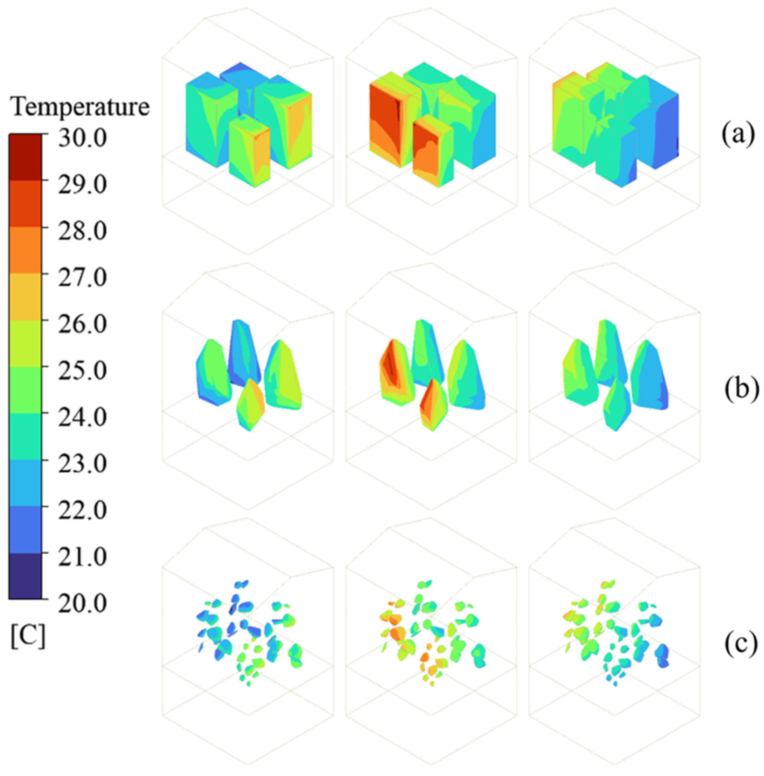
3.4. Comparative Analysis of CFD Simulation of a Small Virtual Greenhouse Model Considering the Fine 3D Structure of Plants

Although different canopy models are used to represent crops, the trend in canopy temperature change remains consistent across the models. The temperature cloud map in Figure 12 reviews significant differences in temperature distribution based on the selected model. The hexahedral porous medium model exhibits distinct regions of high and low temperatures, resulting in substantial temperature differences across the canopy. For the convex hull porous model, the differences are less pronounced compared to the hexahedral porous model. The leaf organ model demonstrates the smoothest transitions in temperature between individual leaves without large temperature discrepancies within the canopy. The average canopy temperature ranges for the hexahedral porous medium, convex cladding porous medium, and leaf organ models are 15.1–30.3 °C, 15.3–29.9 °C, and 15.9–28.8 °C, respectively.

At 10:00, the highest temperatures were observed on the east-facing appeared on the east sunny side while the northwest backlit side recorded the lowest temperatures, and the lowest temperature appeared on the northwest backlit side. The highest temperature value of the hexahedron porous model was 26.8 °C, and the lowest temperature value was 20.1 °C. The highest temperature value of the convex hull porous medium model was 26.4 °C, and the lowest temperature value was 20.5 °C. The highest temperature value of the leaf organ model was 26.1 °C, and the lowest temperature value was 21.1 °C.

At 13:00, the temperature values on the south side of the three models were much higher than those on the north side. The highest temperature value of the hexahedron porous medium model was 29.9 °C, and the lowest temperature value was 22.3 °C. The highest temperature value of the convex hull porous medium model was 29.7 °C, and the lowest temperature value was 22.5 °C. The highest temperature value of the leaf organ model was 27.8 °C, and the lowest temperature value was 22.9 °C.

At 16:00, the canopy temperature on the west side of the three models was higher than that on the east side. The maximum temperature of the hexahedral porous medium model was 26.8 °C, and the minimum temperature was 20.3 °C. The maximum temperature of the convex hull porous medium model was 26.4 °C, and the minimum temperature was 20.7 °C. The maximum temperature of the leaf organ model was 26.1 °C, and the minimum temperature was 21.5 °C.

4. Discussion

4.1. Microclimate Distribution in Solar Greenhouse

The distribution of temperature within a greenhouse is uneven. This variability is influenced not only by external environmental factors but also by the structural characteristics of the greenhouse and crops [38,39]. During the energy exchange between crops, greenhouse enclosures, and sunlight, solar short-wave radiation can penetrate the greenhouse plastic film. Inside the greenhouse, the light waves are converted into long-wave radiation, which is subsequently reflected back by the greenhouse film. This process creates a high-temperature environment inside the greenhouse [40,41].

In the north–south direction, the influence of sunlight during the day results in higher canopy temperatures on the south side of the greenhouse, especially near the greenhouse film. At night, as the external ambient temperature drops, the heat storage and insulation properties of the greenhouse’s north wall become more pronounced, causing higher canopy temperatures on the north side [14,42].

In the east–west direction, the western part of the greenhouse receives light radiation first, causing it to warm up earlier and experience a more significant temperature increase. Conversely, as the west side loses sunlight first, its temperature also begins to drop earlier. During the night, the eastern part of the greenhouse maintains a slightly higher temperature than the western side.

In the vertical direction, the shading effect of the canopy on sunlight produces higher temperatures in the upper canopy compared to the lower canopy during the day. At night, the soil’s heat storage and release properties cause the temperature drop at the 0.5 m canopy height to be smaller than that of the upper canopy, leading to a graduate reduction in vertical temperature difference. These findings are consistent with the research conducted by Mobtaker et al. [43], Xu et al. [44], and Mao et al. [45].

4.2. Necessity of Applying Real Canopy Structure and Future Directions and Challenges

In CFD simulations of the real greenhouse, the convex hull porous model produced results that were closer to the actual values compared to the hexahedral porous model, and the temperature fluctuation range was smaller than that of the hexahedral porous model. Similarly, in simulations of the small greenhouse, the ranges of simulated temperature variations for the hexahedral porous model, the convex hull porous model, and the leaf organ model decreased in that order. This trend is primarily due to the largest spatial volume occupied by the hexahedral porous medium, which has a greater impact on sunlight transmission and airflow in CFD simulation [46]. The convex hull porous medium model occupies a smaller spatial volume than the hexahedral porous medium model. Despite the fact that the simulation results of the latter two models in simulations of the small greenhouse did not exhibit a significant discrepancy compared with those of the hexahedral porous medium model in this experiment, only four plant specimens were employed. Considering the potential cumulative effects of group crops, the convex hull porous medium model still holds great potential for CFD simulations in real greenhouse environments, especially when dealing with crops with larger space volumes, such as cucumbers. The leaf organ model, which has the highest demand for computational resources and shows the smoothest simulated temperature results, best represents the shading effect on sunlight and air retardation, closely matching the real crop growth environment. It is considered the optimal choice if computing resources are sufficient. Currently, there have been applications of 3D CFD models to greenhouse crops such as tomatoes [28] and soybeans [29]. Although the number of simulated plants is relatively small, these studies have proven the broad applicability of the leaf organ model to other greenhouse crops.

The leaf distribution and density of cucumber plants change throughout their growth cycle with plants at different growth stages presenting different degrees of obstruction to airflow. Future models could consider the temporal and spatial variation in porosity to better represent the porous characteristics of crops at different growth stages [29]. Different parts of the plant (such as leaves, stems, and fruits) have different effects on airflow. Leaves tend to have lower permeability, while stems and areas around the fruits may exhibit higher permeability. To improve simulation accuracy, non-uniform permeability should be defined for different regions [28]. During the process of LiDAR point cloud scanning and model generation, some degree of error may naturally occur, as the intricate details of such complex geometries may not be fully captured. The measurement process of sensors can also introduce errors. Additionally, assuming a static canopy structure within a single-day simulation without considering leaf movement or deformation can lead to inaccuracies in the results. Our current CFD model employs a three-row crop layout with the convex hull model and applies the leaf organ model to only four of types crops, both constrained by limited computational resources. Such isolated simulations may not adequately capture the complex interactions across the entire greenhouse. Future research should aim to expand the simulation scope to larger sections of the greenhouse, allowing for a more comprehensive assessment of inter-row interactions.

5. Conclusions

In CFD simulations, modeling greenhouse cucumber plants as porous media can help simulate processes such as airflow, heat transfer, and humidity distribution and provide valuable insights on optimizing the microenvironment inside the greenhouse to improve crop yield and quality. However, the porous media model has limitations in accurately representing the actual temperature distribution that needs further improvement and optimization. In this study, the canopy temperature of the cucumbers at different growth stages was measured using a sensor arrangement. Our analysis indicates the variation in spatial heterogeneity of the canopy temperature of cucumbers in different growth periods. A CFD model of the solar greenhouse was constructed. In the CFD simulations of the real greenhouse, the convex hull porous model yielded results that more closely matched the real-world values than the hexahedral porous model, and it also exhibited a narrower range of temperature fluctuations. In the small greenhouse, the comparison of three crop models using the hexahedral porous model, convex hull porous model, and leaf organ model were conducted. The temperature variation range of the convex hull porous model and the leaf organ model was reduced by 0.6 °C and 2.3 °C, respectively, and both models improved the uniformity of the simulation results.

References

1. Li, T.; Qi, M.; Meng, S. Sixty Years of Facility Horticulture Development in China: Achievements and Prospects. Acta Hortic. Sin. 2022, 10, 2119–2130. [Google Scholar] [CrossRef]
2. Blum, A. Heterosis, Stress, and the Environment: A Possible Road Map towards the General Improvement of Crop Yield. J. Exp. Bot. 2013, 64, 4829–4837. [Google Scholar] [CrossRef]
3. Chen, C.; Ling, H.; Zhai, Z.; Li, Y.; Yang, F.; Han, F.; Wei, S. Thermal Performance of an Active-Passive Ventilation Wall with Phase Change Material in Solar Greenhouses. Appl. Energy 2018, 216, 602–612. [Google Scholar] [CrossRef]
4. Meng, L.; Yang, Q.; Bot, G.P.; Wang, N. Visual Simulation Model for Thermal Environment in Chinese Solar Greenhouse. Trans. Chin. Soc. Agric. Eng. 2009, 25, 164–170. [Google Scholar]
5. Han, Y.; Xue, X.; Luo, X.; Guo, L.; Li, T. Establishment of Estimation Model of Solar Radiation within Solar Greenhouse. Trans. Chin. Soc. Agric. Eng. 2014, 30, 174–181. [Google Scholar]
6. Bournet, P.E.; Rojano, F. Advances of Computational Fluid Dynamics (CFD) Applications in Agricultural Building Modelling: Research, Applications and Challenges. Comput. Electron. Agric. 2022, 201, 107277. [Google Scholar] [CrossRef]
7. Zhou, P.; Wang, S.; Zhou, J.; Hussain, S.A.; Liu, X.; Gao, J.; Huang, G. A Modelling Method for Large-Scale Open Spaces Orientated toward Coordinated Control of Multiple Air-Terminal Units. Build. Simul. 2023, 16, 225–241. [Google Scholar] [CrossRef]
8. Guzmán, C.H.; Carrera, J.L.; Durán, H.A.; Berumen, J.; Ortiz, A.A.; Guirette, O.A.; Arroyo, A.; Brizuela, J.A.; Gómez, F.; Blanco, A.; et al. Implementation of Virtual Sensors for Monitoring Temperature in Greenhouses Using CFD and Control. Sensors 2019, 19, 60. [Google Scholar] [CrossRef] [PubMed]
9. Bartzanas, T.; Boulard, T.; Kittas, C. Effect of Vent Arrangement on Windward Ventilation of a Tunnel Greenhouse. Biosyst. Eng. 2004, 88, 479–490. [Google Scholar] [CrossRef]
10. Ould Khaoua, S.A.; Bournet, P.E.; Migeon, C.; Boulard, T.; Chassériaux, G. Analysis of Greenhouse Ventilation Efficiency Based on Computational Fluid Dynamics. Biosyst. Eng. 2006, 95, 83–98. [Google Scholar] [CrossRef]
11. Saberian, A.; Sajadiye, S.M. The Effect of Dynamic Solar Heat Load on the Greenhouse Microclimate Using CFD Simulation. Renew. Energy 2019, 138, 722–737. [Google Scholar] [CrossRef]
12. Liu, R.; Liu, J.; Liu, H.; Yang, X.; Bárcena, J.F.B.; Li, M. A 3-D Simulation of Leaf Condensation on Cucumber Canopy in a Solar Greenhouse. Biosyst. Eng. 2021, 210, 310–329. [Google Scholar] [CrossRef]
13. Tong, G.; Christopher, D.M.; Zhang, G. New Insights on Span Selection for Chinese Solar Greenhouses Using CFD. Comput. Electron. Agric. 2018, 149, 3–15. [Google Scholar] [CrossRef]
14. Wu, X.; Li, Y.; Jiang, L.; Wang, Y.; Liu, X.; Li, T. A Systematic Analysis of Multiple Structural Parameters of Chinese Solar Greenhouse Based on the Thermal Performance. Energy 2023, 273, 127193. [Google Scholar] [CrossRef]
15. Fatnassi, H.; Bournet, P.E.; Boulard, T.; Roy, J.C.; Molina-Aiz, F.D.; Zaaboul, R. Use of Computational Fluid Dynamic Tools to Model the Coupling of Plant Canopy Activity and Climate in Greenhouses and Closed Plant Growth Systems: A Review. Biosyst. Eng. 2023, 230, 388–408. [Google Scholar] [CrossRef]
16. Boulard, T.; Roy, J.C.; Pouillard, J.B.; Fatnassi, H.; Grisey, A. Modelling of Micrometeorology, Canopy Transpiration and Photosynthesis in a Closed Greenhouse Using Computational Fluid Dynamics. Biosyst. Eng. 2017, 158, 110–133. [Google Scholar] [CrossRef]
17. Xiao, S.; Chai, H.; Shao, K.; Shen, M.; Wang, Q.; Wang, R.; Sui, Y.; Ma, Y. Image-Based Dynamic Quantification of Aboveground Structure of Sugar Beet in Field. Remote Sens. 2020, 12, 269. [Google Scholar] [CrossRef]
18. Chen, B.; Shi, S.; Gong, W.; Zhang, Q.; Yang, J.; Du, L.; Sun, J.; Zhang, Z.; Song, S. Multispectral LiDAR Point Cloud Classification: A Two-Step Approach. Remote Sens. 2017, 9, 373. [Google Scholar] [CrossRef]
19. Sultan Mahmud, M.; Zahid, A.; He, L.; Choi, D.; Krawczyk, G.; Zhu, H.; Heinemann, P. Development of a LiDAR-Guided Section-Based Tree Canopy Density Measurement System for Precision Spray Applications. Comput. Electron. Agric. 2021, 182, 106053. [Google Scholar] [CrossRef]
20. Weiss, U.; Biber, P. Plant Detection and Mapping for Agricultural Robots Using a 3D LIDAR Sensor. Rob. Auton. Syst. 2011, 59, 265–273. [Google Scholar] [CrossRef]
21. Hosoi, F.; Nakabayashi, K.; Omasa, K. 3-D Modeling of Tomato Canopies Using a High-Resolution Portable Scanning Lidar for Extracting Structural Information. Sensors 2011, 11, 2166–2174. [Google Scholar] [CrossRef] [PubMed]
22. Wei, G.; Song, S.; Zhu, B.; Shi, S.; Li, F.; Cheng, X. Multi-Wavelength Canopy LiDAR for Remote Sensing of Vegetation: Design and System Performance. ISPRS J. Photogramm. Remote Sens. 2012, 69, 1–9. [Google Scholar] [CrossRef]
23. Schneider, F.D.; Leiterer, R.; Morsdorf, F.; Gastellu-Etchegorry, J.P.; Lauret, N.; Pfeifer, N.; Schaepman, M.E. Simulating Imaging Spectrometer Data: 3D Forest Modeling Based on LiDAR and in Situ Data. Remote Sens. Environ. 2014, 152, 235–250. [Google Scholar] [CrossRef]
24. Bailey, B.N.; Mahaffee, W.F. Rapid Measurement of the Three-Dimensional Distribution of Leaf Orientation and the Leaf Angle Probability Density Function Using Terrestrial LiDAR Scanning. Remote Sens. Environ. 2017, 194, 63–76. [Google Scholar] [CrossRef]
25. Omasa, K.; Ono, E.; Ishigami, Y.; Shimizu, Y.; Araki, Y. Plant Functional Remote Sensing and Smart Farming Applications. Int. J. Agric. Biol. Eng. 2022, 15, 1–6. [Google Scholar] [CrossRef]
26. Xiao, S.; Ye, Y.; Fei, S.; Chen, H.; Zhang, B.; Li, Q.; Cai, Z.; Che, Y.; Wang, Q.; Ghafoor, A.Z.; et al. High-Throughput Calculation of Organ-Scale Traits with Reconstructed Accurate 3D Canopy Structures Using a UAV RGB Camera with an Advanced Cross-Circling Oblique Route. ISPRS J. Photogramm. Remote Sens. 2023, 201, 104–122. [Google Scholar] [CrossRef]
27. Xiao, S.; Fei, S.; Ye, Y.; Xu, D.; Xie, Z.; Bi, K.; Guo, Y.; Li, B.; Zhang, R.; Ma, Y. 3D Reconstruction and Characterization of Cotton Bolls in Situ Based on UVA Technology. ISPRS J. Photogramm. Remote Sens. 2024, 209, 101–116. [Google Scholar] [CrossRef]
28. Yu, G.; Zhang, S.; Li, S.; Zhang, M.; Benli, H.; Wang, Y. Numerical Investigation for Effects of Natural Light and Ventilation on 3D Tomato Body Heat Distribution in a Venlo Greenhouse. Inf. Process. Agric. 2023, 10, 535–546. [Google Scholar] [CrossRef]
29. Gu, X.; Goto, E. Evaluation of Plant Canopy Microclimates with Realistic Plants in Plant Factories with Artificial Light Using a Computational Fluid Dynamics Model. Build. Environ. 2024, 264, 111876. [Google Scholar] [CrossRef]
30. Wang, Z.; Xu, D.; Lu, T.; Cao, L.; Ji, F.; Zhu, J.; Ma, Y. Quantification of Canopy Heterogeneity and Light Interception Difference within Greenhouse Cucumbers Based on Terrestrial Laser Scanning. Comput. Electron. Agric. 2025, 230, 109879. [Google Scholar] [CrossRef]
31. Kichah, A.; Bournet, P.E.; Migeon, C.; Boulard, T. Corrigendum to “Measurement and CFD Simulation of Microclimate Characteristics and Transpiration of an Impatiens Pot Plant Crop in a Greenhouse” [Biosyst. Eng. 112 (1) (2012) 22–34]. Biosyst. Eng. 2012, 112, 252. [Google Scholar] [CrossRef]
32. Majdoubi, H.; Boulard, T.; Fatnassi, H.; Bouirden, L. Airflow and Microclimate Patterns in a One-Hectare Canary Type Greenhouse: An Experimental and CFD Assisted Study. Agric. For. Meteorol. 2009, 149, 1050–1062. [Google Scholar] [CrossRef]
33. Campen, J.B.; Bot, G.P.A. Determination of Greenhouse-Specific Aspects of Ventilation Using Three-Dimensional Computational Fluid Dynamics. Biosyst. Eng. 2003, 84, 69–77. [Google Scholar] [CrossRef]
34. Nebbali, R.; Roy, J.C.; Boulard, T. Dynamic Simulation of the Distributed Radiative and Convective Climate within a Cropped Greenhouse. Renew. Energy 2012, 43, 111–129. [Google Scholar] [CrossRef]
35. Swinbank, W.C. Long-Wave Radiation from Clear Skies. Q. J. R. Meteorol. Soc. 1963, 89, 339–348. [Google Scholar] [CrossRef]
36. Bartzanas, T.; Boulard, T.; Kittas, C. Numerical Simulation of the Airflow and Temperature Distribution in a Tunnel Greenhouse Equipped with Insect-Proof Screen in the Openings. Comput. Electron. Agric. 2002, 34, 207–221. [Google Scholar] [CrossRef]
37. Molina-Aiz, F.D.; Valera, D.L.; Álvarez, A.J.; Madueño, A. A Wind Tunnel Study of Airflow through Horticultural Crops: Determination of the Drag Coefficient. Biosyst. Eng. 2006, 93, 447–457. [Google Scholar] [CrossRef]
38. Xu, D.; Henke, M.; Li, Y.; Zhang, Y.; Liu, A.; Liu, X.; Li, T. Optimal Design of Light Microclimate and Planting Strategy for Chinese Solar Greenhouses Using 3D Light Environment Simulations. Energy 2024, 302, 131805. [Google Scholar] [CrossRef]
39. Zheng, S.; Cui, N.; Wei, X.; Wang, T.; Bai, Y.; Pei, D.; Fu, S.; Plauborg, F.; Jiao, P. Dynamics, Plant Physiological and Environmental Controls of Energy Exchange in a Grapevine Greenhouse in Northeast China. J. Hydrol. 2024, 637, 131395. [Google Scholar] [CrossRef]
40. Baneshi, M.; Gonome, H.; Maruyama, S. Wide-Range Spectral Measurement of Radiative Properties of Commercial Greenhouse Covering Plastics and Their Impacts into the Energy Management in a Greenhouse. Energy 2020, 210, 118535. [Google Scholar] [CrossRef]
41. Zhang, Y.; Xu, L.; Zhu, X.; He, B.; Chen, Y. Thermal Environment Model Construction of Chinese Solar Greenhouse Based on Temperature–Wave Interaction Theory. Energy Build. 2023, 279, 112648. [Google Scholar] [CrossRef]
42. Li, Y.; Jian, Y.; Wang, S.; Liu, X.; Li, W.; Arıcı, M.; Zhang, L.; Li, W.; Cao, Y. Spatial Temperature Distribution and Ground Thermal Storage in the Plastic Greenhouse: An Experimental and Modeling Study. J. Energy Storage 2024, 77, 109938. [Google Scholar] [CrossRef]
43. Mobtaker, H.G.; Ajabshirchi, Y.; Ranjbar, S.F.; Matloobi, M. Simulation of Thermal Performance of Solar Greenhouse in North-West of Iran: An Experimental Validation. Renew. Energy 2019, 135, 88–97. [Google Scholar] [CrossRef]
44. Xu, K.; Guo, X.; He, J.; Yu, B.; Tan, J.; Guo, Y. A Study on Temperature Spatial Distribution of a Greenhouse under Solar Load with Considering Crop Transpiration and Optical Effects. Energy Convers. Manag. 2022, 254, 115277. [Google Scholar] [CrossRef]
45. Mao, Q.; Li, H.; Ji, C.; Peng, Y.; Li, T. Experimental Study of Ambient Temperature and Humidity Distribution in Large Multi-Span Greenhouse Based on Different Crop Heights and Ventilation Conditions. Appl. Therm. Eng. 2024, 248, 123176. [Google Scholar] [CrossRef]
46. Cui, H.; Wang, C.; Yu, S.; Xin, Z.; Liu, X.; Yuan, J. Two-Stage CFD Simulation of Droplet Deposition on Deformed Leaves of Cotton Canopy in Air-Assisted Spraying. Comput. Electron. Agric. 2024, 224, 109228. [Google Scholar] [CrossRef]
Figure 1. Distribution of observed sensors for temperature within the solar greenhouse.
Agronomy 15 00586 g001
Figure 2. Acquisition of three-dimensional canopy structure of cucumber in solar greenhouse based on ground-based radar: (a) Swarm point clouds; (b) Single-plant point clouds; (c) Convex hull porous model generated by point clouds; (d) Leaf organ model generated by point clouds.
Agronomy 15 00586 g002
Figure 3. Geometric model of the solar greenhouse and its cross-section view: (a) Hexahedral porous; (b) Convex hull porous models.
Agronomy 15 00586 g003
Figure 4. Geometric model of the simulated greenhouse: (a) Hexahedral porous model; (b) Convex hull porous model generated by point clouds; (c) Leaf organ model generated by point clouds.
Agronomy 15 00586 g004
Figure 5. Average measurements of canopy temperature and outdoor temperature during the cucumber growth periods.
Agronomy 15 00586 g005
Figure 6. Canopy temperature at each measurement point (30 September 2023).
Agronomy 15 00586 g006
Figure 7. Canopy temperature of each measurement point at the height of 0.5 m (a) and 1.0 m (b) on 14 October 2023.
Agronomy 15 00586 g007
Figure 8. Canopy temperature at each measurement point at the height of 0.5 m (a), 1.0 m (b), and 1.5 m (c) on 2 November 2023.
Agronomy 15 00586 g008
Figure 9. Comparison between simulated and measured canopy temperature values on 2 November 2023.
Agronomy 15 00586 g009
Figure 10. CFD simulation of canopy temperature distribution at 10:00, 13:00, and 16:00 in solar greenhouse on 2 November 2023. From left to right are simulated results of hexahedral porous and convex hull porous models.
Agronomy 15 00586 g010
Figure 11. Histogram of temperature differences between measured and simulated values in the greenhouse at (a) 10:00, (b) 13:00, and (c) 16:00.
Agronomy 15 00586 g011
Figure 12. CFD simulation of canopy temperature distribution in a simulated greenhouse with Hexahedral porous model (a), Convex hull porous model generated by point clouds (b), and Leaf organ model generated by point clouds (c). From left to right are calculated results at 10:00, 13:00, and 16:00.
Agronomy 15 00586 g012