Article

Joint Effects of Climate and Phenology on Agricultural and Ecological Resource Productivity

1
School of Water Conservancy and Civil Engineering, Northeast Agricultural University, Harbin 150030, China
2
Research Center for Eco-Environment Protection of Songhua River Basin, Northeast Agricultural University, Harbin 150030, China
3
School of Economics and Management, Harbin University of Science and Technology, Harbin 150086, China
*
Author to whom correspondence should be addressed.
These authors contributed equally to this work.
Agronomy 2025, 15(11), 2486; https://doi.org/10.3390/agronomy15112486
Submission received: 30 September 2025 / Revised: 22 October 2025 / Accepted: 23 October 2025 / Published: 26 October 2025
(This article belongs to the Section Agroecology Innovation: Achieving System Resilience)

Abstract

Gross primary productivity (GPP) serves as a critical indicator of carbon uptake in agricultural and natural ecosystems, quantifying the extent of carbon dioxide fixation through photosynthesis. Understanding the influence of climate, phenology, and elevation on GPP is essential for achieving carbon neutrality and ensuring sustainable agricultural and ecosystem management. This study adopts a novel methodology that integrates the Shapley Additive Explanations analysis framework with the XGBoost model (R 4.3.3 package xgboost 1.7.7.1) to elucidate complex nonlinear interactions among the factors under investigation. The results show that from 2001 to 2022, GPP increased at an average rate of 6.77 g C/m2/year, with forests exhibiting the highest productivity (>900 g C/m2) compared to grasslands and croplands (300–600 g C/m2). Phenological changes, such as a 0.44 d/year extension in the growing season and a 0.20 d/year advancement in its peak, highlight the significant impact of climate change on vegetation growth. SHAP analysis further identifies precipitation as the primary driver for croplands, growing season length for forests, and temperature for grasslands. These findings support global initiatives aimed at achieving sustainable development goal 13 (Climate Action) by offering actionable insights for adaptive land use policies and carbon-neutrality strategies.

1. Introduction

Global climate change continues to reshape ecosystem dynamics, and understanding the role of vegetation phenology in carbon sequestration and productivity has become essential for developing effective environmental policies. Vegetation phenology, which includes the length of the growing season (LOS) and the timing of the peak of the growing season (POS), reflects the temporal patterns of vegetation growth and plays a critical role in mediating the exchange of energy, carbon, and water between the biosphere and the atmosphere [1,2,3]. It is increasingly recognized as a fundamental indicator for assessing the impacts of climate change on vegetation dynamics and serves as a vital proxy for key ecosystem functions, enabling the evaluation of terrestrial ecosystem productivity [4,5,6,7,8]. While traditional field observations provide valuable insights into phenological responses, their spatial and temporal limitations present significant challenges for large-scale policy assessment [9]. Remote sensing technologies, particularly MODIS-derived products, have become indispensable for analyzing phenological patterns across extensive regions with high temporal resolution [10,11,12]. Satellite imagery, offering comprehensive global coverage and consistent repeatability, has become pivotal in deriving vegetation characteristics [13,14]. The MCD12Q2 product, known for its robust performance in monitoring vegetation dynamics, is especially well-suited for examining the interactions between phenology, climate, and ecosystem productivity at regional scales [15,16,17].
Vegetation productivity serves as a pivotal indicator of ecosystem functioning, with gross primary productivity (GPP) playing a fundamental role in comprehending the carbon balance of ecosystems and evaluating vegetation responses to global changes [18,19]. Accurately capturing the spatiotemporal variations in GPP and interannual fluctuations in carbon sinks is crucial for ecosystem management and climate mitigation [20,21]. Climate shifts have significantly impacted the timing of key phenological events. An earlier start of the growing season (SOS) and a delayed end of the growing season (EOS) result in an extended LOS, subsequently leading to increased GPP due to the prolonged LOS [22]. Simultaneously, the POS plays an important role in shaping the seasonal dynamics of GPP [23]. Climate-induced changes in phenological parameters can indirectly impact vegetation GPP, thereby influencing the carbon sequestration capabilities of ecosystems [24,25]. Previous studies have identified temperature (Tem) and precipitation (Pre) as the primary drivers of phenological shifts [6,26].
Ecosystems exhibit varied responses to climatic factors and elevation (Ele) gradients [27,28]. Consequently, both GPP and vegetation phenology play critical roles in shaping carbon sequestration in terrestrial ecosystems [29,30,31]. Although numerous studies have investigated the impacts of climate-phenology interactions on ecosystem productivity, most have focused on individual climatic variables or relied on conventional statistical methods that assume linear relationships [32]. For instance, recent studies have employed statistical models to assess the effect of temperature and precipitation on GPP [33,34], yet these approaches often neglect nonlinear interactions among multiple drivers. Moreover, while some studies have examined the influence of elevation on phenology and productivity, its interactive effects with other climatic variables remain insufficiently understood [35,36]. Capturing such nonlinear dynamics and quantifying the relative importance of each factor continues to pose a significant challenge. The integration of eXtreme Gradient Boosting (XGBoost) with Shapley Additive Explanations (SHAP) provides a robust framework for uncovering these complex relationships [37,38]. XGBoost excels in handling high-dimensional and nonlinear data, and when coupled with SHAP, it enables not only the detection of intricate interaction patterns but also the interpretation of individual variable contributions. This combined approach has been effectively applied across diverse domains, including human health [38,39], socio-economic sciences [40], and vegetation dynamics [41,42]. Nevertheless, its potential to reveal climate-ecological interactions underlying ecosystem productivity remains underexploited.
This study employs the XGBoost-SHAP framework to elucidate the nonlinear interactions between phenological factors, climate drivers, and GPP. This novel methodology enables the precise quantification of individual contributions and interactions among variables, providing deeper insights compared to traditional correlation analyses. The primary objectives of this research are to (1) analyze the spatiotemporal distribution of phenological indices and GPP and (2) assess the impacts of phenological and environmental factors on GPP across various ecosystems. By integrating advanced analytical methodologies with actionable insights, this study aims to bridge the gap between environmental science and policy-making, thereby contributing to the achievement of carbon neutrality in global ecosystems and providing replicable methodologies for similar ecosystems globally.

2. Materials and Methods

2.1. Study Area

The Songhua River Basin (SRB) is situated in Northeast China (119°52′ to 132°31′ E, 41°42′ to 51°38′ N), spanning an area of approximately 561,200 km2 across four provincial administrative regions: Heilongjiang, Jilin, Liaoning, and the Inner Mongolia Autonomous Region [43] (Figure 1). The primary land use categories within the basin consist of cultivated land and grassland, with forest land being the second most prevalent. The vast geographical expanse and considerable elevation variation in the SRB create a complex meteorological and hydrological landscape, which is essential for informing regional environmental policy and management [44]. The annual average Tem ranges from −4.41 to 7.28 °C, with a spatial distribution that decreases from south to north. Moreover, the overall elevation of the basin varies between 48 and 2576 m, while the annual average precipitation ranges from 351 to 1143 mm. In most regions within the SRB, there is a predominant single growth cycle, typically occurring from April to October, during which vegetation reaches its peak in July and August.

2.2. Datasets

To meet the data requirements for our models, we compiled multiple datasets from diverse sources, as summarized in Table 1. The analysis focused on GPP estimates derived from the MODIS (MOD17A2) product aboard NASA’s Terra satellite, covering the period from 2001 to 2022. A comprehensive assessment was conducted on the complete pixel dataset across the SRB, enabling a systematic evaluation of ecosystem diversity and complexity throughout the entire study region, rather than relying on fragmented or localized sampling. To validate the MODIS GPP estimates, we compared them with ground-based measurements from FLUXNET stations. Due to the limited spatial distribution of FLUXNET stations within the SRB, we selected data from two representative sites in China, Changling Station (CN-Cng) and Changbai Mountain Station (CN-Cha), for verification purposes (https://fluxnet.org/data/fluxnet2015-dataset, accessed on 15 May 2025). Correlation analysis revealed determination coefficients (R2) of 0.8893 and 0.8346 between the MODIS GPP estimates and observed values at CN-Cng and CN-Cha, respectively, supporting the reliability and applicability of the MODIS GPP data for the SRB.
The characteristic variables included LOS, POS, Pre, Tem, and Ele. LOS and POS, as phenological parameters, help elucidate the impact of the plant growth cycle on GPP [45], while Pre and Tem are primary climatic drivers influencing phenological changes [46]. Additionally, variations in Ele significantly affect regional climate patterns and vegetation types [47]. Therefore, when analyzing the influence of phenology on GPP, incorporating Ele as an auxiliary variable allows for a more accurate simulation of GPP distribution patterns across different ecosystems. To ensure consistent spatial resolution, LULC and GPP datasets were resampled to 1 km × 1 km.

2.3. Methods

To achieve the research objectives, this study employed an integrative methodological framework that combines remote sensing data, machine learning techniques, and SHAP method approaches [41,42,48]. The overall methodological framework of this study is illustrated in Figure 2, where we utilized the MODIS dataset to establish the GPP and phenological datasets within the SRB (Steps 1 and 2). Subsequently, we evaluated the correlation between phenological indices and GPP while considering climate and terrain factors (Step 3). Finally, by employing the XGBoost-SHAP model, we assessed how phenological indices impact GPP under the influence of climate and terrain factors (Step 4). This methodological framework not only ensures robust quantification of the drivers influencing GPP but also offers actionable insights into the interactions among climate, phenology, and productivity, providing a valuable foundation for policy-relevant ecological management.

2.3.1. Data Preparation

We utilized MODIS satellite imagery spanning from 2001 to 2022, constituting a 22-year time series dataset. The data were processed to extract annual GPP, phenological indicators (LOS and POS), and environmental variables (Pre, Tem, and Ele) at a spatial resolution of 1 km × 1 km. The extracted data were organized into a spatiotemporal matrix, with each pixel representing an independent observation. Ele data were integrated to account for topographical variability, while phenological and climatic variables captured the seasonal and interannual variability affecting GPP. Data preprocessing involved resampling all datasets to a consistent spatial resolution, ensuring the alignment of climate, phenology, and productivity data.

2.3.2. Model Construction: Extreme Gradient Boosting Model Framework

To analyze the intricate relationships among phenological, climatic, and topographical factors, an XGBoost model was employed [49]. XGBoost is a machine learning algorithm renowned for its efficiency in processing large datasets and capturing nonlinear interactions between predictors and target variables. It effectively integrates tree-based learning methods, making it particularly suitable for capturing the complex nonlinear dependencies present in the data [46]. This model was chosen for its ability to mitigate potential overfitting and provide robust predictions [50].

2.3.3. Explainable Predictions: SHAP Method

The SHAP method can be utilized to calculate the marginal contribution of all features to the model output and interpret black-box models at both global and local levels [49]. We employed SHAP values, which provide insights into the marginal contribution of each predictor variable toward the target variable [51]. The combination of XGBoost and SHAP not only allows for quantifying the contribution of each predictor variable to the target variable but also facilitates analyzing interactions among different predictor variables and their effects on the target variable. For every prediction sample, the model generates a prediction value. By utilizing the SHAP method, it becomes feasible to compute the contribution of feature values related to influential factors toward the dependent variable [38]. The SHAP value was obtained using Equation (1).
φ j = S x 1 x p x i S ! p S 1 ! p ! f x S x j f x S
where φj denotes the contribution of the jth feature, x represents the feature value vector of the instance to be explained, and p indicates the number of features. Moreover, fx(S) refers to the prediction of feature values in subset S, marginalized over features not included in S.
Subsequently, the additive feature attribution method was utilized to calculate the SHAP value according to Equation (2).
g Z = φ 0 + j = 1 M φ j Z j
where g denotes the interpretation model, z′∈{0,1} indicates whether a feature is present ( Z j = 1) or not ( Z j = 0) in the calculation, and M is the total number of features.
The SHAP method offers a means of providing global interpretation [52]. It enables the measurement of the importance of SHAP characteristics in influencing factors through the calculation formula presented in Equation (3).
I S H A P j = 1 n i = 1 n φ j i
where j and i are the input variable and data sample, respectively, and n is the number of samples.
SHAP was applied to quantify feature contributions (SHAP values), main effects independent of other inputs (SHAP main effects values), and pairwise interaction effects (SHAP interaction values). Feature importance was ranked by the mean absolute SHAP value for each predictor. After identifying the main influential factors, we analyze their individual and interactive effects on GPP using SHAP values. The XGBoost model was computed using R 4.3.3 package xgboost 1.7.7.1, while the computation of the SHAP model was performed using R 4.3.3 package shapviz 0.9.3.

2.3.4. Statistical Validation

To validate the findings, we conducted complementary statistical analyses, including Theil-Sen trend analysis and the Mann–Kendall test (M–K test), to evaluate temporal trends in GPP and phenological indicators [53]. Partial correlation analyses were further performed to isolate the effects of individual variables while controlling for potential confounders. Detailed equations and validation metrics are provided in Supporting Information (SI). Trend detection, the M–K test, correlation and partial correlation analyses, as well as the GeoDetector model based on optimized parameters, were performed using R 4.3.3 package GD 10.8. Line graphs, box plots, and bar charts were generated using Origin 2025.

3. Results

3.1. Spatio-Temporal Changes in the GPP and Vegetation Phenology

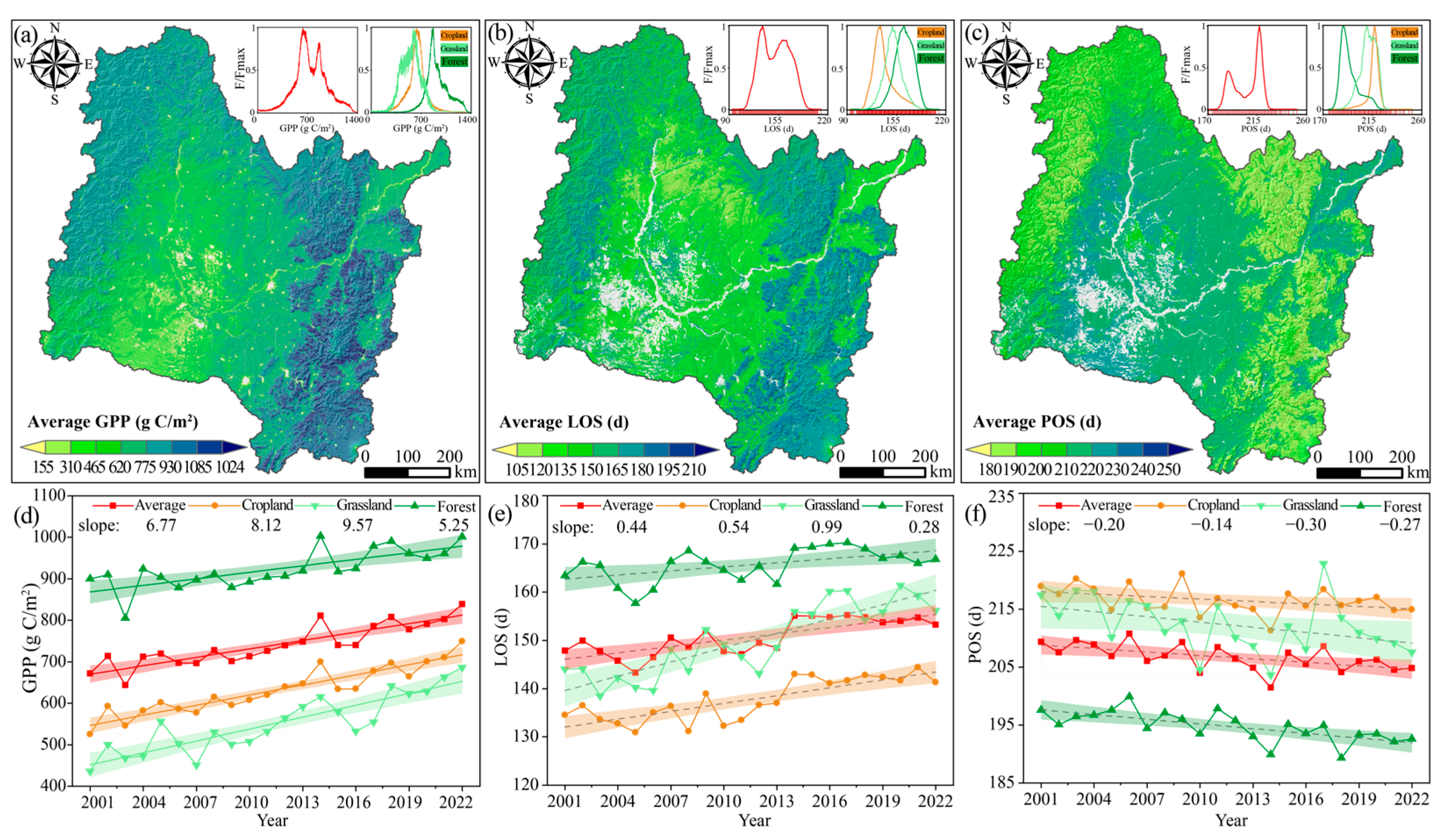
The average gross primary productivity (GPP) of the study region from 2001 to 2022 was recorded as 741 g C/m2, with forested areas consistently exhibiting higher GPP values (often surpassing 900 g C/m2 in southeastern regions), while cropland-dominated areas displayed comparatively lower values (ranging between 300 and 600 g C/m2) (Figure 3a). During the 22-year study period, GPP exhibited a significant upward trend, with an average annual increase rate of 6.77 g C/m2/year. Specifically, cropland, grassland, and forest areas demonstrated substantial increases in GPP at rates of 8.12, 9.57, and 5.25 g C/m2/year, respectively (Figure 3d). The average length of growing season (LOS) and peak of growing season (POS) were recorded as 151 days (Figure 3b) and 206 days (Figure 3c), respectively; moreover, LOS showed a consistent annual extension of 0.44 d/year (Figure 3e), and POS continued to advance by 0.20 d/year (Figure 3f). Differences in LOS and POS values were observed across land use types: forests exhibited the longest LOS (165 days) and the earliest POS (194 days), while croplands had the shortest LOS (138 days) and latest POS (216 days). These phenological patterns displayed spatial variations, with an extension trend of LOS from high to low latitudes and a delayed initiation followed by advancement pattern observed particularly in grassland and cropland areas.
The Mann–Kendall (M–K) test revealed that 96.8% of GPP pixels exhibited increasing trends, with statistically significant increases observed in 73.4% of cases (Figure S1a,d). Similarly, lengthening trends were observed in 81.2% of LOS pixels, with a significant extension found in 46.3%, predominantly in low-altitude cropland and grassland areas (Figure S1b,e). In contrast, approximately 68.8% of POS pixels demonstrated advancement trends, particularly noticeable in high-altitude forested regions, where a significant advancement was observed in 25.2% of pixels (Figure S1c,f).

3.2. Correlation Analysis of GPP with Vegetation Phenology and Environmental Factors

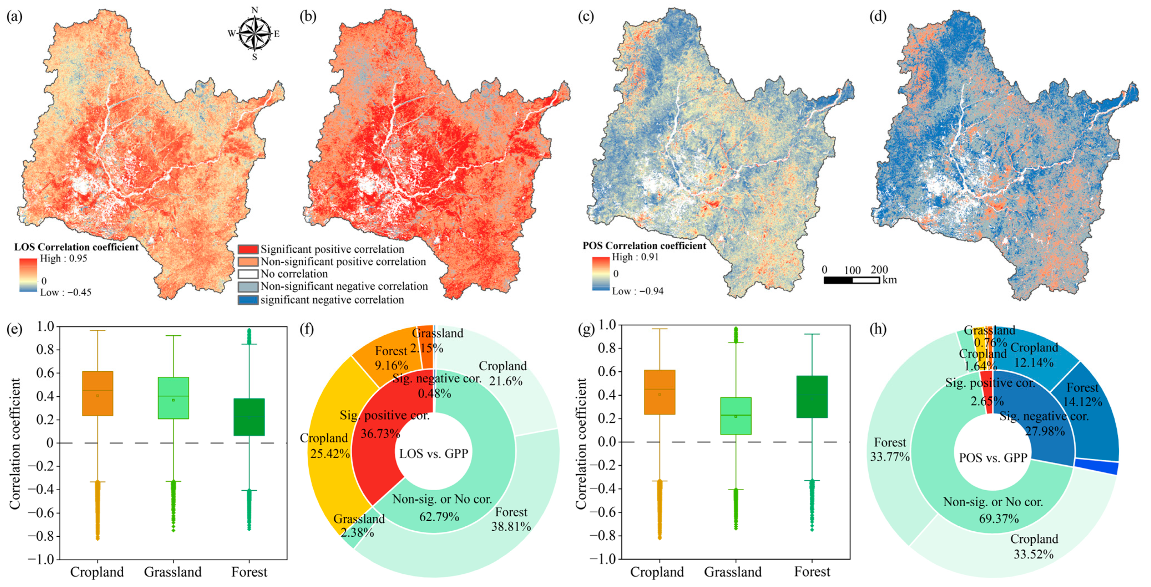
Spatial correlation analysis revealed a predominantly positive relationship between GPP and LOS (Figure 4a,b), while GPP was mainly negatively correlated with POS (Figure 4c,d). These findings suggest that an extended LOS generally enhances GPP across the study area, whereas POS has a constraining effect in certain ecosystems. Among different vegetation types, cropland-dominated regions demonstrated the strongest positive correlation between LOS and GPP, followed by grassland and forest areas (Figure 4e,f). In contrast, the correlations between POS and GPP varied among vegetation types, with cropland and forest showing stronger relationships compared to grassland areas (Figure 4g,h). To further explore these relationships, we conducted a partial correlation analysis controlling for elevation (Ele), temperature (Tem), and precipitation (Pre): (a) without any control factor (C0); (b) using Ele as a control factor (C1); (c) using Tem and Pre as control factors (C2); and (d) using Ele, Pre, and Tem as control factors (C3) (Figure S2). The results consistently showed that, regardless of the controlled conditions used in the analysis (Ele, Tem, and Pre), LOS exhibited a positive partial correlation with GPP, particularly in forest ecosystems, where this correlation remained strong across all controlled conditions (C1–C3). On the other hand, POS maintained a negative correlation with GPP, especially under C1 and C2 conditions, indicating that Ele and climate factors modulate the influence of POS on GPP to varying degrees (Figure S2). Controlling for Ele, Tem, and Pre enhanced the observed correlations between LOS and GPP, suggesting that interactions among climate factors and Ele amplify the positive impact of an extended growing season. In grassland ecosystems, Ele consistently exhibited a negative effect on GPP (Figure S2b), while in cropland and forest ecosystems, the positive influence of LOS on GPP remained robust (Figure S2a,c).

3.3. SHAP Analysis of GPP Driving Factors, Main Effects, and Interaction Effects

The relationship between vegetation GPP and phenology, including LOS and POS, poses a challenge for characterization solely through simple correlation analysis. This approach may introduce uncertainty and limit further exploration of the association [54]. In this study, we utilized Shapley Additive Explanations (SHAP) values derived from the SHAP-XGBoost model to quantify the influence magnitude of various factors on GPP across all pixels from 2001 to 2022 (Figure 5). A negative SHAP value indicates a reduction in GPP due to a specific influencing factor, while a positive value suggests an increase. In cropland ecosystems, Pre is identified as the most influential factor, followed by LOS, whereas POS has a relatively lower impact (Figure 5a). In grassland ecosystems, Tem emerges as the most significant influencing factor, with a significantly higher impact compared to others, while POS and LOS are found to be the least influential factors (Figure 5b). In forest ecosystems, LOS and Pre are identified as the two main influencing factors, whereas Ele has the lowest impact on ecosystem dynamics (Figure 5c). However, due to the wide range of variations in Pre and LOS, GPP exhibits significant dynamic fluctuations, resulting in pronounced left and right tails in the SHAP values. In cropland ecosystems (Figure 5d), the SHAP values for LOS and Ele exhibit unimodal distributions, primarily centered around the mean, with limited variability in the positive range. Conversely, Pre demonstrates a more symmetric pattern, with SHAP values evenly distributed across both positive and negative ranges, reflecting a balanced impact. In grassland ecosystems (Figure 5e), Tem and Ele significantly contribute to GPP improvement, as indicated by predominantly positive SHAP values. LOS and POS show concentrated distributions near the mean, suggesting a relatively consistent effect, while Pre maintains a balanced distribution without significant deviation. In forest ecosystems (Figure 5f), LOS and POS exhibit strong positive contributions, whereas Pre shows neutral impact reflected by balanced SHAP value distributions. To ensure the robustness of our findings, we conducted a year-by-year SHAP analysis, which revealed remarkable consistency with the SHAP analysis presented in the main text (Figures S3–S5).
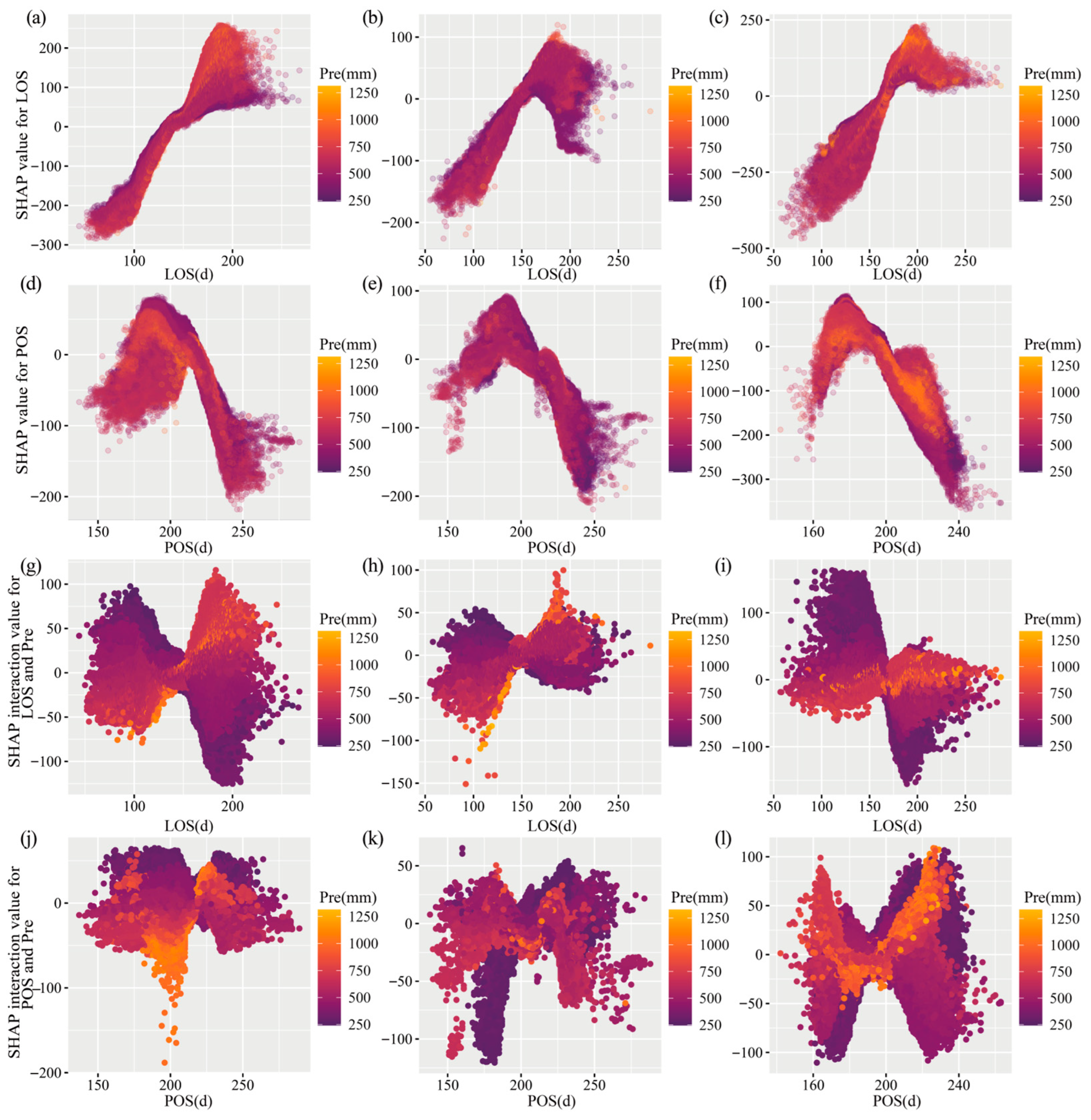
We employ SHAP dependency and interaction plots to examine the influence of key driving factors on the relationship between vegetation phenology (LOS and POS) and GPP. In different ecosystems, a shift from GPP inhibition to enhancement observed when LOS exceeds 120 days in croplands, 150 days in grasslands, and 170 days in forests, evidenced by a transition in SHAP values from positive to negative (Figure 6). Among these thresholds, cropland LOS exerts the most pronounced effect on GPP at approximately 170 days (Figure 6a), whereas both grassland (Figure 6b) and forest (Figure 6c) ecosystems exhibit peak influence at an LOS of around 180 days. However, the response patterns between POS and LOS show limited consistency. In cropland ecosystems, POS exhibited a positive value between 170 and 220 days, but its effect on GPP shifted from promotion to inhibition when exceeding 230 days (Figure 6d). In grasslands, the influence of POS on GPP became ambiguous within the 180 to 220 day range (Figure 6e). In forests, POS promoted GPP before reaching 200 days, but inhibited it thereafter (Figure 6f). Moreover, the SHAP dependency plots clearly reveal the interaction between two variables. A distinct positive correlation between LOS and Pre is evident from the vertical spread in the plots: higher LOS values correspond to higher Pre values (Figure 6g–i). Conversely, lower LOS values are generally associated with reduced Tem, resulting in lower SHAP values (Figure S6a–c,g–i). From an ecological perspective across ecosystems, grasslands exhibit less pronounced interaction effects between LOS/POS and Pre compared to croplands (Figure 6j) and forests (Figure 6k,l). However, the coupling between LOS and Pre is stronger than that between POS and Pre, with notable variation across ecosystem types. Generally, lower POS values are associated with decreased Tem levels, leading to reduced SHAP values (Figure S6d–f,j–l). Annual analysis consistently reveals positive effects in forest ecosystems when LOS approaches 170 days, whereas croplands and grasslands exhibit greater volatility during periods of low Pre. Furthermore, the impact of POS gradually shifts from promotion to inhibition under high-Tem conditions, highlighting its sensitivity to interannual climate variability (Figures S7–S18).
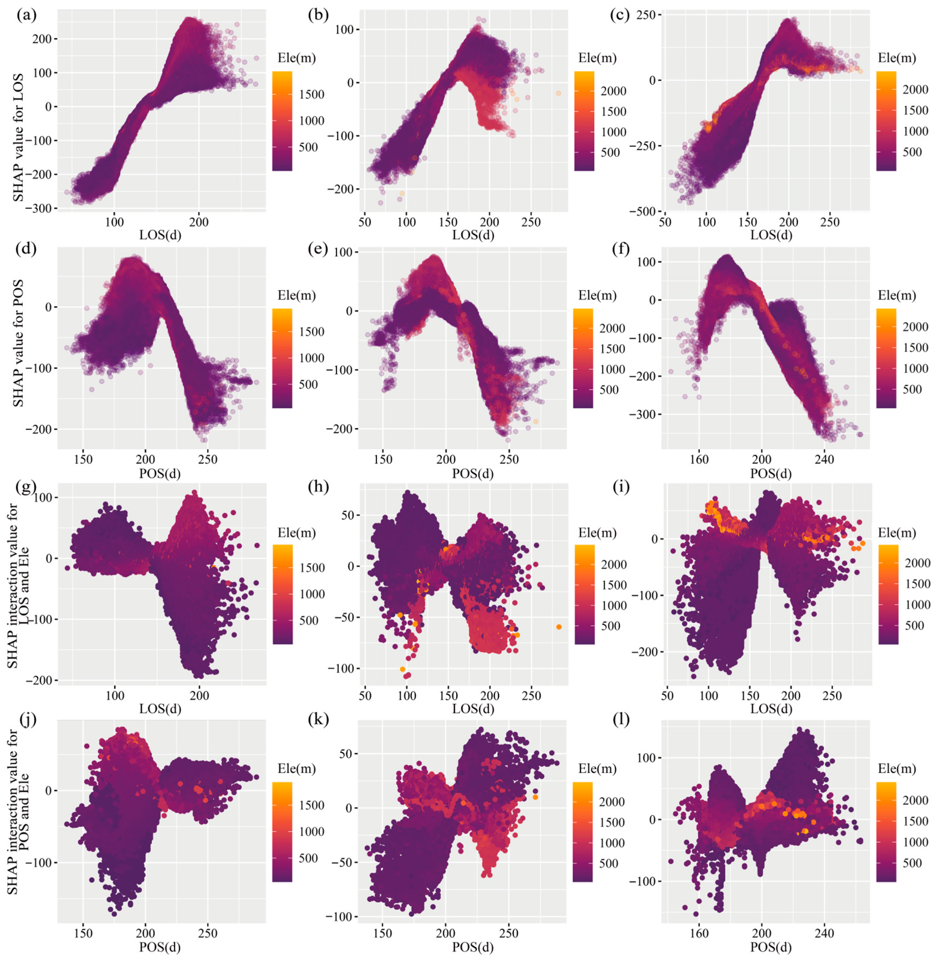
The dependency relationship between GPP and LOS (Figure 7a–c), as well as POS (Figure 7d–f), remains unaffected by variations in Ele, which exhibits both positive and negative SHAP values in regions of high and low Ele. Across all ecosystems, the SHAP values of LOS and POS do not exhibit any distinct directional bias with changes in Ele. From an ecosystem perspective, the interaction between LOS and Ele strengthens with increasing Ele in croplands (Figure 7g). In grassland ecosystems, the SHAP values of LOS and Ele increase with higher Ele but decrease with lower Ele (Figure 7h), while in forest ecosystems, the interaction effect diminishes consistently across all Ele ranges (Figure 7i). The interaction pattern between POS and Ele mirrors that of LOS (Figure 7j–l). Overall, we observe that the sensitivity response of most GPP is significantly influenced by the interaction between Tem and Pre, whereas the impact of Ele interaction on vegetation phenology sensitivity response is not significant. The annual and overall analyses reveal that the influence of LOS and POS on GPP fluctuates depending on Ele (Figures S19–S24). Notably, in high-altitude regions, the inflection points of SHAP values show more pronounced positive and negative transitions.
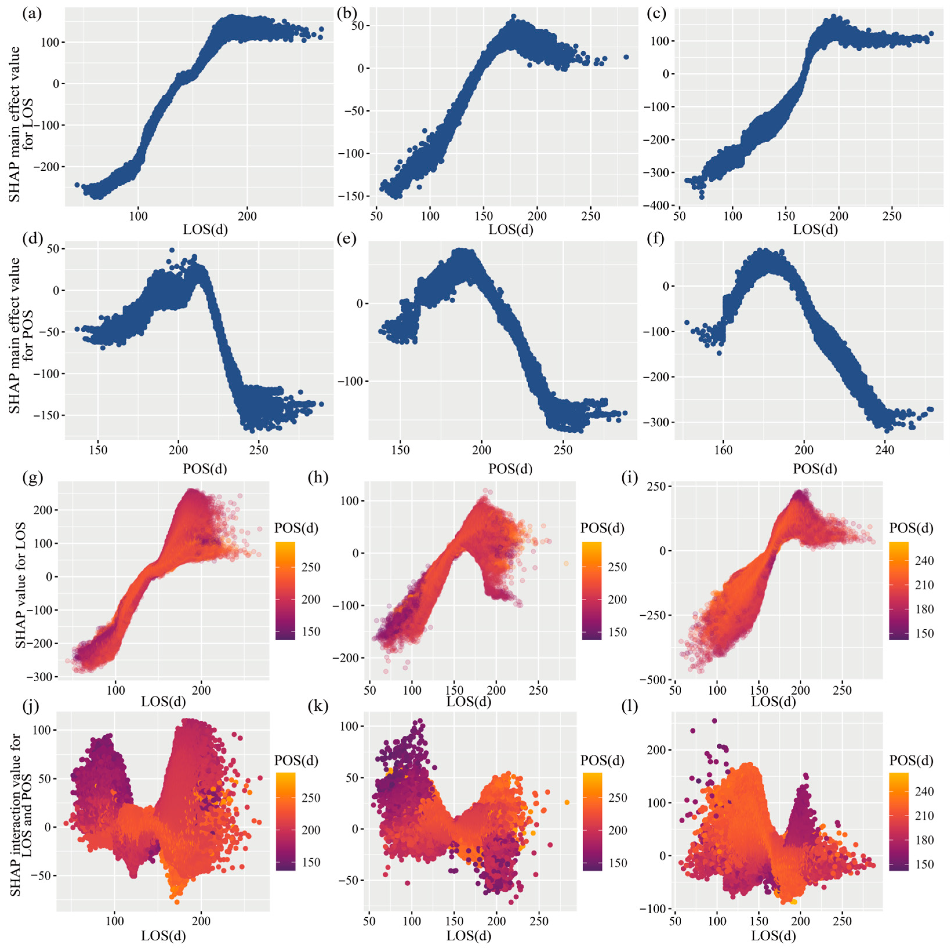
In cropland (Figure 8a) and grassland ecosystems (Figure 8b), an increase in LOS is associated with a positive impact on GPP, as indicated by the upward trend in SHAP main effect values. However, in regions with high LOS, fluctuations in SHAP values reflect the influence of environmental factors and data uncertainty. In forest ecosystems (Figure 8c), the SHAP main effect value initially increases with LOS, reaching a peak at approximately 200 days before declining, suggesting reduced photosynthetic efficiency during extended growing seasons. The relationship between the SHAP main effect values and POS is shown in Figure 8d–f. Overall, an increase in POS leads to a rise in the SHAP main effect values, which then gradually decline after reaching a peak. Notably, these peaks exhibit certain fluctuations: around 220 days in cropland ecosystems, 190–200 days in grassland ecosystems, and 180 days in forest ecosystems. Following their respective peaks, fluctuations are observed during the decline of SHAP values, underscoring the complex nature of photosynthesis across diverse ecosystems. From the perspective of dynamic ecosystem response, SHAP values for forest ecosystems show relatively minor year-to-year fluctuations, indicating high stability amidst interannual variations. However, annual analyses of phenology in cropland and grassland ecosystems (Figures S25–S30) reveal significant interannual fluctuations in the high-value range of SHAP values, while maintaining a similar overall influence of LOS and POS on GPP. Additionally, the peak position of POS on GPP varies annually, with some years showing lower peak values in grassland ecosystems due to their sensitivity to environmental changes, whereas forest ecosystems demonstrate higher stability with smaller fluctuations in SHAP values over time.
Figure 8g–i depict the association between LOS and POS. The highest SHAP value of GPP typically corresponds to longer LOS and higher POS. In cropland ecosystems (Figure 8j), an increase in POS is linked to a decrease in the SHAP interaction value as LOS increases, whereas a decrease in POS leads to an increase in the SHAP interaction value with rising LOS, accompanied by local fluctuations. In forest ecosystems (Figure 8l), when there is a combination of high POS and low LOS or low POS and high LOS, the SHAP interaction value tends to be high. However, when both POS and LOS are high, resource constraints may cause a decrease in the SHAP interaction value. In grassland ecosystems (Figure 8k), compared to other ecosystems, the significance level of the interaction effect appears relatively lower, with a narrower range of SHAP values observed.
The relative importance of driving factors, quantified by mean absolute SHAP values and ranked in Table 2, identifies ecosystem–specific primary drivers of GPP: precipitation in croplands, temperature in grasslands, and growing season length in forests. This distinct pattern underscores the necessity for tailored ecosystem management strategies.
To validate the reliability of this conclusion, we applied the GeoDetector method, which is grounded in spatial heterogeneity theory and informed by the second law of geography, to analyze the factors driving the spatial variation in GPP across three ecosystems. Detailed computational procedures for the GeoDetector are provided in SI. The results are consistent with those obtained from XGBoost showing that Pre and LOS are dominant drivers in cropland and forest areas, whereas Tem exerts the primary influence in grasslands (Table 3). This independent analytical approach provides robust support for the SHAP analysis, reinforcing the identification of ecosystem-specific controls on GPP within the study region.

4. Discussion

4.1. Spatiotemporal Patterns of GPP and Vegetation Phenology (LOS and POS)

The multi-year average GPP in the SRB exhibits a distinct geographical pattern corresponding to the distribution of various ecosystems (Figure 3a). The combination of Theil Sen trend analysis and the M-K test effectively captures the spatiotemporal variations in GPP [55], while demonstrating robustness against outliers. However, the observed spatial heterogeneity in GPP also reflects varying levels of exposure to climatic risks, which directly informs the development of policy frameworks under Sustainable Development Goal (SDG) 13 (Climate Action) [56]. For example, cropland and grassland areas, which are highly sensitive to changes in Pre and Tem, could benefit from climate adaptation policies focused on optimizing water resources and implementing sustainable land use planning [57,58]. The central area of the SRB is predominantly characterized by cropland and grassland, while forests dominate its surrounding regions, thereby shaping the spatial distribution pattern of GPP with respect to land use (Figure 1b). There is strong evidence that across a wide range of taxonomic and functional groups, vegetation growth is significantly influenced by climatic factors [59], and species are adapting to climate change by modifying their phenology and geographical distributions [60,61]. Previous studies have also confirmed that vegetation growth is highly influenced by climate factors. A favorable hydrothermal environment plays a crucial role in providing essential resources for plant growth, while adequate soil moisture ensures normal photosynthesis under sufficient CO2 concentration and light [62]. Additionally, ample soil moisture facilitates nutrient transport processes [63,64]. Furthermore, Tem is another important climate factor affecting vegetation growth, particularly with regard to changes in vegetation phenology and LOS (Figure S3). Tem shows a negative correlation with POS, indicating that higher Tem advances POS (Figure S31). Increasing Tem promotes enzyme activity involved in photosynthesis, thereby enhancing both the intensity of plant photosynthesis and organic matter uptake by plants [65,66].
Pre can compensate for water deficits and exert uniform effects on LOS (Figure S32) and POS (Figure S33). Previous studies have demonstrated the significant sensitivity of vegetation phenology to Pre [67,68], indicating that supplementary rainfall can alleviate soil water deficits caused by greening processes [69], and that aridification induces systematic and abrupt changes in multiple ecosystem attributes [70]. Moreover, Zhou et al. [71] reported a correlation between accelerated vegetation growth and an earlier onset of spring vegetative development. Consistent with these findings, our trend analysis of SOS also supports this observation (Figure S34). Additionally, it should be noted that the influence of phenology on GPP depends on Tem and Pre, albeit with slight variations across different ecosystems. This finding aligns with the research conducted by Chen and Zhang [35]. With global warming, plants may experience an earlier rise in Tem, leading to an earlier emission of SOS signals, thereby exacerbating vegetation loss [6]. However, due to incomplete understanding of the impact mechanisms of Tem, Pre, and their interactions on phenology, as well as unclear responses of different ecosystems to climate change, further investigation and analysis are required to comprehend the main reasons for these differences [72].

4.2. Influence of Phenology on the Relationship Between Climate and GPP

According to the spatial distribution characteristics of Pre and Tem (Figure S35), the patterns of LOS, POS, and GPP in the SRB exhibit similarities with the distribution of Pre and Tem (Figure 3). The ongoing global warming trend has led to significant changes in vegetation phenology [73], with a progressive advancement of SOS (Figure S34) and a delayed EOS (Figure S36), resulting in a substantial prolongation of LOS in the SRB. The observed spatiotemporal correlations between phenological indices (LOS and POS) and GPP, moderated by climate factors, underscore the complex dynamics governing ecosystem productivity. These findings align closely with SDG 13 by highlighting the critical role of climate-driven phenological shifts in shaping vegetation responses. Previous studies have demonstrated that this extension profoundly impacts vegetation growth by providing an extended period for photosynthesis, thereby facilitating increased accumulation of organic matter and energy [74,75,76]. Photosynthesis plays a fundamental role in plant development, as it supplies essential nutrients and energy for growth and overall progression. Consequently, this extended phenological period enhances photosynthetic efficiency and increases the accumulation of photosynthetic products, which corresponds to the results of de Souza et al. [77] and Zhai et al. [78]. Therefore, alterations in vegetation phenology represent responses to climate change while serving as crucial mechanisms for ecosystem self-regulation and adaptation to environmental conditions [23].

4.3. The Importance of Ele to GPP Distribution

Vegetation growth is influenced by both climate change and geographical environmental factors [59,79]. Ele reflects topographic changes that directly impact the distribution of water, nutrients, air conditions, heat, and other environmental factors. These factors play a decisive role in vegetation growth and development [80,81,82]. Previous studies have found that thermal conditions (radiation and Tem) limit plant growth in high-latitude or high-altitude areas, where reduced radiation negatively affects plant productivity [83]. As a crucial topographic factor, Ele influences the distribution of GPP by shaping ecosystem distribution. The GPP of various ecosystems is influenced by phenological, climatic, and topographical factors, leading to distinct feedbacks. Our analysis reveals that cropland and forest ecosystems are primarily affected by Pre and LOS, while grasslands are influenced by Tem (Figure 5). As Pre decreases under low Pre conditions, an increase in LOS leads to a decrease in the SHAP interaction value between LOS and Pre for GPP (Figure 6), mainly due to drought-induced reductions in GPP levels [84]. Additionally, drought events often result in elevated carbon emissions caused by reduced humidity levels, decreased Pre rates, higher Tem, increased radiation exposure, as well as fire disturbances [85,86]. Plant phenology plays a crucial role in determining the growth period and intensity of photosynthesis activity among plants [87]. The threshold effect may manifest as either a mutation or attenuation of specific plant phenological phenomena on GPP after reaching a certain level [88].

4.4. Uncertainty and Future Research

This study quantitatively investigates the influence of vegetation phenology, climate, and altitude on changes in GPP within the SRB. It lays a foundation for further exploring the feedback effects of GPP changes on phenology and the environment, as well as their implications for carbon cycling. Moreover, it provides theoretical support for developing ecological restoration and management strategies in China’s major grain-producing regions, ecological security barriers, and typical basins in cold areas. However, uncertainties remain due to computational limitations, data collection challenges, and limitations of analytical methods. First, it should be noted that our findings are limited to the specific timeframe under investigation and cannot be extrapolated over longer durations. Second, while our focus lies on annual-scale growth patterns, it is important to recognize that short-term variations in vegetation response to climate change exhibit high dependence on temporal scales [89]. The XGBoost–SHAP framework effectively captures nonlinear relationships, yet it is subject to certain limitations. The substantial computational demands of XGBoost hinder its scalability when applied to large datasets [90], and SHAP-based interpretation introduces additional computational overhead, making real-time large-sample applications challenging. Although SHAP enhances model explainability [91], its interpretive reliability may diminish in the presence of deep decision trees or high-dimensional feature spaces, where interactions become increasingly complex. Future research should aim to overcome these constraints by investigating more computationally efficient machine learning models that maintain strong interpretability without compromising predictive performance. Additionally, extending the XGBoost-SHAP framework to incorporate additional environmental variables, such as soil moisture and atmospheric CO2 concentrations, could enhance the accuracy and robustness of GPP predictions under diverse climate scenarios.

5. Conclusions

This study accomplished its objectives by quantitatively analyzing the spatiotemporal patterns of vegetation phenology and GPP in the Songhua River Basin, as well as evaluating the influences of phenological and environmental factors on GPP across diverse ecosystems. The key findings are summarized as follows:
(1)
The integration of the XGBoost-SHAP framework effectively uncovered nonlinear relationships and quantified the individual contributions of driving factors on GPP, thereby overcoming the limitations of traditional linear analyses. This approach enabled a mechanistic understanding of ecosystem-specific drivers: precipitation was the dominant factor in croplands, temperature in grasslands, and length of growing season (LOS) in forests.
(2)
The study demonstrated that vegetation phenology plays a critical mediating role in linking climate change to ecosystem productivity. An extended LOS and an earlier peak of the growing season (POS) were found to significantly enhance carbon sequestration capacity. Furthermore, the interactions between phenological indicators and environmental factors revealed distinct threshold effects and varied across ecosystem types, indicating strong ecosystem dependency.
(3)
The research establishes a transferable analytical framework for understanding complex ecosystem dynamics, delivering actionable insights for regional carbon budget assessments and sustainable ecosystem management. The methodology and findings hold significant relevance for designing targeted climate adaptation strategies in agricultural and forest ecosystems within temperate regions.

Supplementary Materials

The following supporting information can be downloaded at: https://www.mdpi.com/article/10.3390/agronomy15112486/s1, Figure S1: Spatial trends in GPP, LOS, and POS; Figure S2: Partial correlation analysis of GPP with vegetation phenology and environmental factors; Figure S3: SHAP values of GPP driving factors in crop ecosystem; Figure S4: SHAP values of GPP driving factors in grass ecosystem; Figure S5: SHAP values of GPP driving factors in forest ecosystem; Figure S6: SHAP dependence plot and SHAP interaction plot across for GPP of crop, grass, and forest; Figure S7: SHAP dependence plot of LOS versus its SHAP value along the Pre for crop ecosystem; Figure S8: SHAP dependence plot of LOS versus its SHAP value along the Pre for grass ecosystem; Figure S9: SHAP dependence plot of LOS versus its SHAP value along the Pre for forest ecosystem; Figure S10: SHAP dependence plot of POS versus its SHAP value along the Pre for crop ecosystem; Figure S11: SHAP dependence plot of POS versus its SHAP value along the Pre for grass ecosystem; Figure S12: SHAP dependence plot of POS versus its SHAP value along the Pre for forest ecosystem; Figure S13: SHAP dependence plot of LOS versus its SHAP value along the Tem for crop ecosystem; Figure S14: SHAP dependence plot of LOS versus its SHAP value along the Tem for grass ecosystem; Figure S15: SHAP dependence plot of LOS versus its SHAP value along the Tem for forest ecosystem; Figure S16: SHAP dependence plot of POS versus its SHAP value along the Tem for crop ecosystem; Figure S17: SHAP dependence plot of POS versus its SHAP value along the Tem for grass ecosystem; Figure S18: SHAP dependence plot of POS versus its SHAP value along the Tem for forest ecosystem; Figure S19: SHAP dependence plot of LOS versus its SHAP value along the Ele for crop ecosystem; Figure S20: SHAP dependence plot of LOS versus its SHAP value along the Ele for grass ecosystem; Figure S21: SHAP dependence plot of LOS versus its SHAP value along the Ele for forest ecosystem; Figure S22: SHAP dependence plot of POS versus its SHAP value along the Ele for crop ecosystem; Figure S23: SHAP dependence plot of POS versus its SHAP value along the Ele for forest ecosystem; Figure S24: SHAP dependence plot of POS versus its SHAP value along the Ele for grass ecosystem; Figure S25: SHAP main effect plot of LOS on GPP for crop ecosystem; Figure S26: SHAP main effect plot of LOS on GPP for grass ecosystem; Figure S27: SHAP main effect plot of LOS on GPP for forest ecosystem; Figure S28: SHAP main effect plot of POS on GPP for crop ecosystem; Figure S29: SHAP main effect plot of POS on GPP for grass ecosystem; Figure S30: SHAP main effect plot of POS on GPP for forest ecosystem; Figure S31: Correlation between POS and Tem; Figure S32: Correlation between LOS and Pre; Figure S33: Correlation between POS and Pre; Figure S34: Distribution of SOS spatial change trend; Figure S35: Spatial distribution of climatic factors; Figure S36: Distribution of EOS spatial change trend. References [35,92,93] are cited in the Supplementary file.

Author Contributions

Conceptualization, S.C.; methodology, S.C. and Z.J.; software, Z.J. and Z.S.; validation, L.G. and F.Z.; formal analysis, F.Z.; investigation, F.Z. and Z.S.; resources, S.C.; data curation, Z.J.; writing—original draft preparation, F.Z. and Z.J.; writing—review and editing, S.C. and L.G.; visualization, L.G. and Z.S.; supervision, S.C.; project administration, S.C.; funding acquisition, S.C. All authors have read and agreed to the published version of the manuscript.

Funding

This research was funded by the National Key Research and Development Program of China (grant number 2024YFD1501702), the Distinguished Youth Science Foundation of Heilongjiang Province, China (grant number JQ2023E001) and Young Leading Talents of Northeast Agricultural University, China (grant number NEAU2023QNLJ-013 and NEAU2024QNLJ-01).

Data Availability Statement

The original contributions presented in the study are included in the article/supplementary material, further inquiries can be directed to the corresponding author.

Conflicts of Interest

The authors declare no conflicts of interest.

References

  1. Liu, F.; Wang, X.C.; Zhang, Y.C.; Shen, Y.J. Novel metrics for assessing vegetation phenology from hydrological processes: Comparison with photosynthetic phenology. Agric. For. Meteorol. 2024, 358, 110245. [Google Scholar] [CrossRef]
  2. Dronova, I.; Taddeo, S. Remote sensing of phenology: Towards the comprehensive indicators of plant community dynamics from species to regional scales. J. Ecol. 2022, 110, 1460–1484. [Google Scholar] [CrossRef]
  3. Díaz, J.G.; Gutierrez-Bustillo, A.M.; Rojo, J. Influence of urbanisation on the phenology of evergreen coniferous and deciduous broadleaf trees in Madrid (Spain). Landsc. Urban Plan. 2023, 235, 104760. [Google Scholar] [CrossRef]
  4. Buermann, W.; Forkel, M.; O’Sullivan, M.; Sitch, S.; Friedlingstein, P.; Haverd, V.; Jain, A.K.; Kato, E.; Kautz, M.; Lienert, S.; et al. Widespread seasonal compensation effects of spring warming on northern plant productivity. Nature 2018, 562, 110–114. [Google Scholar] [CrossRef]
  5. Park, T.; Chen, C.; Macias-Fauria, M.; Tommervik, H.; Choi, S.; Winkler, A.; Bhatt, U.S.; Walker, D.A.; Piao, S.L.; Brovkin, V.; et al. Changes in timing of seasonal peak photosynthetic activity in northern ecosystems. Glob. Change Biol. 2019, 25, 2382–2395. [Google Scholar] [CrossRef]
  6. Shen, M.G.; Wang, S.P.; Jiang, N.; Sun, J.P.; Cao, R.Y.; Ling, X.F.; Fang, B.; Zhang, L.; Zhang, L.H.; Xu, X.Y.; et al. Plant phenology changes and drivers on the Qinghai-Tibetan Plateau. Nat. Rev. Earth Env. 2022, 3, 717. [Google Scholar] [CrossRef]
  7. You, W.B.; Xian, Z.Y.; Zhou, G.Y.; Agathokleous, E.; Yu, Z. Sensitivity of forest phenology in China varies with proximity to forest edges. For. Ecosyst. 2023, 10, 100144. [Google Scholar] [CrossRef]
  8. Shen, X.J.; Shen, M.G.; Wu, C.Y.; Peñuelas, J.; Ciais, P.; Zhang, J.Q.; Freeman, C.; Palmer, P.I.; Liu, B.H.; Henderson, M.; et al. Critical role of water conditions in the responses of autumn phenology of marsh wetlands to climate change on the Tibetan Plateau. Glob. Change Biol. 2024, 30, e17097. [Google Scholar] [CrossRef] [PubMed]
  9. Ge, Q.S.; Dai, J.H.; Cui, H.J.; Wang, H.J. Spatiotemporal variability in start and end of growing season in China related to climate variability. Remote Sens. 2016, 8, 433. [Google Scholar] [CrossRef]
  10. McNairn, H.; Jiao, X.F.; Pacheco, A.; Sinha, A.; Tan, W.K.; Li, Y.F. Estimating canola phenology using synthetic aperture radar. Remote Sens. Environ. 2018, 219, 196–205. [Google Scholar] [CrossRef]
  11. Wang, X.F.; Xiao, J.F.; Li, X.; Cheng, G.D.; Ma, M.G.; Zhu, G.F.; Arain, M.A.; Black, T.A.; Jassal, R.S. No trends in spring and autumn phenology during the global warming hiatus. Nat. Commun. 2019, 10, 2389. [Google Scholar] [CrossRef] [PubMed]
  12. Silveira, E.M.O.; Pidgeon, A.M.; Persche, M.; Radeloff, V.C. Remotely-sensed phenoclusters of Wisconsin’s forests, shrublands, and grasslands for biodiversity applications. For. Ecol. Manag. 2024, 561, 121878. [Google Scholar] [CrossRef]
  13. Zeng, L.L.; Wardlow, B.D.; Xiang, D.X.; Hu, S.; Li, D.R. A review of vegetation phenological metrics extraction using time-series, multispectral satellite data. Remote Sens. Environ. 2020, 237, 111511. [Google Scholar] [CrossRef]
  14. Mo, Y.H.; Chen, S.Z.; Wu, Z.F.; Tang, J.; Fu, Y.S. The advancement in spring vegetation phenology in the northern hemisphere will reverse after 2060 under future moderate warming scenarios. Earths Future 2024, 12, e2023EF003788. [Google Scholar] [CrossRef]
  15. Cui, S.; Du, X.L.; Jia, Z.Y.; Fu, Q.; Liu, D. Spatiotemporal dynamics of carbon-related ecosystem services: Unraveling socio-ecological drivers and leveraging bundles for sustainable spatial zoning. J. Environ. Manag. 2025, 394, 127359. [Google Scholar] [CrossRef]
  16. Shi, D.D.; Jiang, Y.; Li, W.Q.; Wen, Y.; Wu, F.; Zhao, S.D. Spatial-temporal heterogeneity of spring phenology in boreal forests as estimated by satellite solar-induced chlorophyll fluorescence and vegetation index. Agric. For. Meteorol. 2024, 346, 109888. [Google Scholar] [CrossRef]
  17. Kloos, S.; Klosterhalfen, A.; Knohl, A.; Menzel, A. Decoding autumn phenology: Unraveling the link between observation methods and detected environmental cues. Glob. Change Biol. 2024, 30, e17231. [Google Scholar] [CrossRef] [PubMed]
  18. Liu, H.Y.; Wang, Z.; Wang, Z.Y.; Zeng, Y.Z.; Xue, P.; Zhang, M.Y. Stability of the ecosystem gross primary productivity increasing in Chinese forestry ecological engineering area. Agric. Ecosyst. Environ. 2023, 356, 108636. [Google Scholar] [CrossRef]
  19. Yu, G.R.; Chen, Z.; Wang, Y.P. Carbon, water and energy fluxes of terrestrial ecosystems in China. Agric. For. Meteorol. 2024, 346, 109890. [Google Scholar] [CrossRef]
  20. Zeng, Z.Q.; Wu, W.X.; Li, Y.M.; Huang, C.; Zhang, X.Q.; Peñuelas, J.; Zhang, Y.; Gentine, P.; Li, Z.L.; Wang, X.Y.; et al. Increasing meteorological drought under climate change reduces terrestrial ecosystem productivity and carbon storage. One Earth 2023, 6, 1326–1339. [Google Scholar] [CrossRef]
  21. Zhu, X.J.; Yu, G.R.; Chen, Z.; Zhang, W.K.; Han, L.; Wang, Q.F.; Qi, H.; Yang, M.; Liu, Z.G.; Dou, X.J.; et al. Ecosystem responses dominate the trends of annual gross primary productivity over terrestrial ecosystems of China during 2000–2020. Agric. For. Meteorol. 2023, 343, 109758. [Google Scholar] [CrossRef]
  22. Li, P.; Sun, M.; Liu, Y.X.; Ren, P.X.; Peng, C.H.; Zhou, X.L.; Tang, J.Y. Response of vegetation photosynthetic phenology to urbanization in Dongting Lake Basin, China. Remote Sens. 2021, 13, 3722. [Google Scholar] [CrossRef]
  23. Huang, Z.; Zhou, L.; Chi, Y.G. Spring phenology rather than climate dominates the trends in peak of growing season in the Northern Hemisphere. Glob. Change Biol. 2023, 29, 4543–4555. [Google Scholar] [CrossRef]
  24. Higgins, S.I.; Conradi, T.; Muhoko, E. Shifts in vegetation activity of terrestrial ecosystems attributable to climate trends. Nat. Geosci. 2023, 16, 147–153. [Google Scholar] [CrossRef]
  25. Gampe, D.; Zscheischler, J.; Reichstein, M.; O’Sullivan, M.; Smith, W.K.; Sitch, S.; Buermann, W. Increasing impact of warm droughts on northern ecosystem productivity over recent decades. Nat. Clim. Change 2023, 13, 1272. [Google Scholar] [CrossRef]
  26. Currier, C.M.; Sala, O.E. Precipitation versus temperature as phenology controls in drylands. Ecology 2022, 103, e3793. [Google Scholar] [CrossRef]
  27. Cui, S.; Du, X.L.; Jia, Z.Y.; Fu, Q.; Liu, D. Ecosystem service value estimation and ecological security pattern in Heilongjiang Province. Environ. Sci. 2024, 45, 6489–6500. (In Chinese) [Google Scholar] [CrossRef]
  28. Dong, S.K.; Li, S.; Xu, Y.D.; Shen, H.; Song, H.J.; Wu, Z.F.; Wu, S.N.; Zhou, B.R.; Li, F. Different responses of alpine plants to natural climate change reduced coexistence through phenological niche overlap. Sci. Total Environ. 2023, 892, 164522. [Google Scholar] [CrossRef]
  29. Wang, X.W.; Lei, H.M.; Li, J.D.; Qu, Y.P.; Kong, D.D.; Huo, Z.L. Climate and management impacts on the spatiotemporal dynamics of water-carbon fluxes in the North China Plain. Agric. Ecosyst. Environ. 2023, 343, 108270. [Google Scholar] [CrossRef]
  30. Xie, X.Y.; Zhao, W.; Yin, G.F. TAVIs: Topographically adjusted vegetation index for a reliable proxy of gross primary productivity in mountain ecosystems. IEEE Trans. Geosci. Remote Sens. 2023, 62, 4400412. [Google Scholar] [CrossRef]
  31. Ren, Y.J.; Qiu, J.X.; Zeng, Z.Z.; Liu, X.P.; Sitch, S.; Pilegaard, K.; Yang, T.Y.; Wang, S.; Yuan, W.P.; Jain, A.K. Earlier spring greening in Northern Hemisphere terrestrial biomes enhanced net ecosystem productivity in summer. Commun. Earth Environ. 2024, 5, 122. [Google Scholar] [CrossRef]
  32. Leng, Y.; Li, W.; Ciais, P.; Sun, M.X.; Zhu, L.; Yue, C.; Chang, J.F.; Yao, Y.T.; Zhang, Y.; Zhou, J.X.; et al. Forest aging limits future carbon sink in China. One Earth 2024, 7, 822–834. [Google Scholar] [CrossRef]
  33. Gong, E.J.; Zhang, J.; Wang, Z.H.; Hu, Q.F.; Bai, H.Y.; Wang, J. Global comparison of temperature and water stress representations in light use efficiency models for gross primary productivity estimation. ISPRS J. Photogramm. 2025, 230, 275–288. [Google Scholar] [CrossRef]
  34. Shi, J.Y.; Liu, M.X.; Li, Y.; Guan, C.X. Response of total primary productivity of vegetation to meteorological drought in arid and semi-arid regions of China. J. Arid Environ. 2025, 228, 105346. [Google Scholar] [CrossRef]
  35. Chen, X.; Zhang, Y.P. Impacts of climate, phenology, elevation and their interactions on the net primary productivity of vegetation in Yunnan, China under global warming. Ecol. Indic. 2023, 154, 110533. [Google Scholar] [CrossRef]
  36. Vitasse, Y.; Signarbieux, C.; Fu, Y.S.H. Global warming leads to more uniform spring phenology across elevations. Proc. Natl. Acad. Sci. USA 2018, 115, 1004–1008. [Google Scholar] [CrossRef] [PubMed]
  37. Rodriguez-Perez, R.; Bajorath, J. Interpretation of machine learning models using shapley values: Application to compound potency and multitarget activity predictions. J. Comput. Aid. Mol. Des. 2020, 34, 1013–1026. [Google Scholar] [CrossRef]
  38. Lundberg, S.M.; Erion, G.; Chen, H.; DeGrave, A.; Prutkin, J.M.; Nair, B.; Katz, R.; Himmelfarb, J.; Bansal, N.; Lee, S.-I. From local explanations to global understanding with explainable AI for trees. Nat. Mach. Intell. 2020, 2, 56–67. [Google Scholar] [CrossRef]
  39. Li, W.; Huang, G.; Tang, N.; Lu, P.; Jiang, L.; Lv, J.; Qin, Y.; Lin, Y.; Xu, F.; Lei, D. Effects of heavy metal exposure on hypertension: A machine learning modeling approach. Chemosphere 2023, 337, 139435. [Google Scholar] [CrossRef]
  40. Parsa, A.B.; Movahedi, A.; Taghipour, H.; Derrible, S.; Mohammadian, A.K. Toward safer highways, application of XGBoost and SHAP for real-time accident detection and feature analysis. Accid. Anal Prev. 2020, 136, 105405. [Google Scholar] [CrossRef]
  41. Descals, A.; Verger, A.; Yin, G.F.; Filella, I.; Peñuelas, J. Local interpretation of machine learning models in remote sensing with SHAP: The case of global climate constraints on photosynthesis phenology. Int. J. Remote Sens. 2023, 44, 3160–3173. [Google Scholar] [CrossRef]
  42. Xie, J.L.; Yin, G.F.; Xie, Q.Y.; Wu, C.Y.; Yuan, W.P.; Zeng, Y.L.; Verger, A.; Descals, A.; Filella, I.; Peñuelas, J. Shifts in climatic limitations on global vegetation productivity unveiled by Shapley Additive Explanation: Reduced temperature but increased water limitations. J. Geophys. Res. Biogeosci. 2024, 129, e2024JG008354. [Google Scholar] [CrossRef]
  43. Jia, Z.Y.; Guo, L.; Fu, Q.; Liu, D.; Du, X.L.; Cui, S. Integrating ecological networks and multi-scenario optimization: A novel framework for constructing ecological security patterns. Agric. Ecol. Environ. 2025, 1, e007. [Google Scholar]
  44. Cui, S.; Jia, Z.Y.; Guo, L.; Fu, Q.; Liu, D. Impacts of extreme climate events at different altitudinal gradients on vegetation NPP in Songhua River basin. Environ. Sci. 2024, 45, 275–286. (In Chinese) [Google Scholar] [CrossRef]
  45. Liu, Z.J.; Jiao, L.M.; Lian, X.H. Changes in compound extreme events and their impacts on cropland productivity in China, 1985–2019. Earth’s Future 2025, 13, e2024EF005038. [Google Scholar] [CrossRef]
  46. Li, C.; Zou, Y.Y.; He, J.F.; Zhang, W.; Gao, L.L.; Zhuang, D.F. Response of vegetation phenology to the interaction of temperature and precipitation changes in Qilian Mountains. Remote Sens. 2022, 14, 1248. [Google Scholar] [CrossRef]
  47. Chmura, H.E.; Kharouba, H.M.; Ashander, J.; Ehlman, S.M.; Rivest, E.B.; Yang, L.H. The mechanisms of phenology: The patterns and processes of phenological shifts. Ecol. Monogr. 2019, 89, e01337. [Google Scholar] [CrossRef]
  48. Gao, M.D.; Piao, S.L.; Chen, A.P.; Yang, H.; Liu, Q.; Fu, Y.S.H.; Janssens, I.A. Divergent changes in the elevational gradient of vegetation activities over the last 30 years. Nat. Commun. 2019, 10, 2970. [Google Scholar] [CrossRef]
  49. García, M.V.; Aznarte, J.L. Shapley additive explanations for NO2 forecasting. Ecol. Inform. 2020, 56, 101039. [Google Scholar] [CrossRef]
  50. Wang, S.; Peng, H.; Hu, Q.; Jiang, M. Analysis of runoff generation driving factors based on hydrological model and interpretable machine learning method. J. Hydrol. Reg. Stud. 2022, 42, 101139. [Google Scholar] [CrossRef]
  51. Zhang, W.Q.; Luo, G.P.; Hamdi, R.; Ma, X.M.; Li, Y.Z.; Yuan, X.L.; Li, C.F.; Ling, Q.; Hellwich, O.; Termonia, P.; et al. Can gross primary productivity products be effectively evaluated in regions with few observation data? GIScience Remote Sens. 2023, 60, 2213489. [Google Scholar] [CrossRef]
  52. Carlsson, L.S.; Samuelsson, P.B.; Jonsson, P.G. Interpretable machine learning-tools to interpret the predictions of a machine learning model predicting the electrical energy consumption of an electric arc furnace. Steel Res. Int. 2020, 91, 2000053. [Google Scholar] [CrossRef]
  53. Jia, Z.Y.; Guo, L.; Cui, S.; Fu, Q.; Liu, D. Spatial-temporal evolution of NPP and its response to extreme climate in Songhua River basin. South-North Water Transf. Water Sci. Technol. 2024, 22, 131–147. (In Chinese) [Google Scholar] [CrossRef]
  54. Lin, Z.Q.; Liu, Y.Y.; Wen, Z.M.; Chen, X.; Han, P.D.; Zheng, C.; Yao, H.B.; Wang, Z.J.; Shi, H.J. Spatial-temporal variation characteristics and driving factors of net primary production in the Yellow River Basin over multiple time scales. Remote Sens. 2023, 15, 5273. [Google Scholar] [CrossRef]
  55. Wang, A.; Zhang, M.M.; Chen, E.Q.; Zhang, C.; Han, Y.J. Impact of seasonal global land surface temperature (LST) change on gross primary production (GPP) in the early 21st century. Sustain. Cities Soc. 2024, 110, 105572. [Google Scholar] [CrossRef]
  56. Han, D.N.; Yu, D.Y.; Qiu, J.X. Assessing coupling interactions in a safe and just operating space for regional sustainability. Nat. Commun. 2023, 14, 1369. [Google Scholar] [CrossRef]
  57. Poppe Terán, C.; Naz, B.S.; Graf, A.; Qu, Y.; Hendricks Franssen, H.J.; Baatz, R.; Ciais, P.; Vereecken, H. Rising water-use efficiency in European grasslands is driven by increased primary production. Commun. Earth Environ. 2023, 4, 95. [Google Scholar] [CrossRef]
  58. Yang, Y.; Tilman, D.; Jin, Z.N.; Smith, P.; Barrett, C.B.; Zhu, Y.G.; Burney, J.; D’Odorico, P.; Fantke, P.; Fargione, J.; et al. Climate change exacerbates the environmental impacts of agriculture. Science 2024, 385, 6713. [Google Scholar] [CrossRef] [PubMed]
  59. Peng, W.F.; Kuang, T.T.; Tao, S. Quantifying influences of natural factors on vegetation NDVI changes based on geographical detector in Sichuan, western China. J. Clean. Prod. 2019, 233, 353–367. [Google Scholar] [CrossRef]
  60. Doorga, J.R.S. Climate change and the fate of small islands: The case of Mauritius. Environ. Sci. Policy 2022, 136, 282–290. [Google Scholar] [CrossRef]
  61. Lenoir, J.; Gégout, J.C.; Marquet, P.A.; de Ruffray, P.; Brisse, H. A significant upward shift in plant species optimum elevation during the 20th century. Science 2008, 320, 1768–1771. [Google Scholar] [CrossRef]
  62. Zheng, Z.Z.; Li, L.F.; Biederman, J.A.; Wang, Y.F.; Guan, S.T.; Li, C.J.; Wen, F.Q.; Liu, Y.; Xiong, Y.Q.; Qian, R.Y.; et al. Ecosystem CO2 flux responses to extreme droughts depend on interaction of seasonal timing and plant community composition. J. Ecol. 2024, 112, 2198–2211. [Google Scholar] [CrossRef]
  63. Cusack, D.F.; Dietterich, L.H.; Sulman, B.N. Soil respiration responses to throughfall exclusion are decoupled from changes in soil moisture for four tropical forests, suggesting processes for ecosystem models. Glob. Biogeochem. Cycles 2023, 37, e2022GB007473. [Google Scholar] [CrossRef]
  64. Knapp, A.K.; Condon, K.V.; Folks, C.C.; Sturchio, M.A.; Griffin-Nolan, R.J.; Kannenberg, S.A.; Gill, A.S.; Hajek, O.L.; Siggers, J.A.; Smith, M.D. Field experiments have enhanced our understanding of drought impacts on terrestrial ecosystems-But where do we go from here? Funct. Ecol. 2024, 38, 76–97. [Google Scholar] [CrossRef]
  65. Ye, C.C.; Sun, J.; Liu, M.; Xiong, J.N.; Zong, N.; Hu, J.; Huang, Y.; Duan, X.W.; Tsunekawa, A. Concurrent and Lagged Effects of Extreme Drought Induce Net Reduction in Vegetation Carbon Uptake on Tibetan Plateau. Remote Sens. 2020, 12, 2347. [Google Scholar] [CrossRef]
  66. Piao, S.L.; Friedlingstein, P.; Ciais, P.; Viovy, N.; Demarty, J. Growing season extension and its impact on terrestrial carbon cycle in the Northern Hemisphere over the past 2 decades. Glob. Biogeochem. Cy. 2007, 21, 2006GB002888. [Google Scholar] [CrossRef]
  67. Wu, L.Z.; Ma, X.F.; Dou, X.; Zhu, J.T.; Zhao, C.Y. Impacts of climate change on vegetation phenology and net primary productivity in arid Central Asia. Sci. Total Environ. 2021, 796, 149055. [Google Scholar] [CrossRef]
  68. Fang, H.S.; Sha, M.Q.; Xie, Y.C.; Lin, W.J.; Qiu, D.; Tu, J.G.; Tan, X.C.; Li, X.L.; Sha, Z.Y. Shifted Global Vegetation Phenology in Response to Climate Changes and Its Feedback on Vegetation Carbon Uptake. Remote Sens. 2023, 15, 2288. [Google Scholar] [CrossRef]
  69. Lian, X.; Piao, S.L.; Li, L.Z.X.; Li, Y.; Huntingford, C.; Ciais, P.; Cescatti, A.; Janssens, I.A.; Peñuelas, J.; Buermann, W.; et al. Summer soil drying exacerbated by earlier spring greening of northern vegetation. Sci. Adv. 2020, 6, eaax0255. [Google Scholar] [CrossRef]
  70. Berdugo, M.; Delgado-Baquerizo, M.; Soliveres, S.; Hernández-Clemente, R.; Zhao, Y.C.; Gaitan, J.J.; Gross, N.; Saiz, H.; Maire, V.; Lehman, A.; et al. Global ecosystem thresholds driven by aridity. Science 2020, 367, 787–790. [Google Scholar] [CrossRef]
  71. Zhou, X.C.; Geng, X.J.; Yin, G.D.; Hänninen, H.; Hao, F.H.; Zhang, X.; Fu, Y.S.H. Legacy effect of spring phenology on vegetation growth in temperate China. Agric. For. Meteorol. 2020, 281, 107845. [Google Scholar] [CrossRef]
  72. Ossola, A.; Lin, B.B. Making nature-based solutions climate-ready for the 50 °C world. Environ. Sci. Policy 2021, 123, 151–159. [Google Scholar] [CrossRef]
  73. Cong, N.; Wang, T.; Nan, H.J.; Ma, Y.C.; Wang, X.H.; Myneni, R.B.; Piao, S.L. Changes in satellite-derived spring vegetation green-up date and its linkage to climate in China from 1982 to 2010: A multimethod analysis. Glob. Change Biol. 2013, 19, 881–891. [Google Scholar] [CrossRef]
  74. Guo, J.T.; Hu, Y.M. Spatiotemporal Variations in Satellite-Derived Vegetation Phenological Parameters in Northeast China. Remote Sens. 2022, 14, 705. [Google Scholar] [CrossRef]
  75. Hussain, S.; Ulhassan, Z.; Brestic, M.; Zivcak, M.; Zhou, W.J.; Allakhverdiev, S.I.; Yang, X.H.; Safdar, M.E.; Yang, W.Y.; Liu, W.G. Photosynthesis research under climate change. Photosynth. Res. 2021, 150, 5–19. [Google Scholar] [CrossRef] [PubMed]
  76. Ueyama, M.; Iwata, H.; Harazono, Y. Autumn warming reduces the CO2 sink of a black spruce forest in interior Alaska based on a nine-year eddy covariance measurement. Glob. Change Biol. 2014, 20, 1161–1173. [Google Scholar] [CrossRef] [PubMed]
  77. de Souza, M.A.; de Andrade, L.I.F.; Gago, J.; Pereira, E.G. Photoprotective mechanisms and higher photorespiration are key points for iron stress tolerance under heatwaves in rice. Plant Sci. 2024, 342, 112031. [Google Scholar] [CrossRef]
  78. Zhai, B.Y.; Hu, Z.Y.; Sun, S.Q.; Tang, Z.S.; Wang, G.X. Characteristics of photosynthetic rates in different vegetation types at high-altitude in mountainous regions. Sci. Total Environ. 2024, 907, 168071. [Google Scholar] [CrossRef]
  79. Qu, S.; Wang, L.C.; Lin, A.W.; Yu, D.Q.; Yuan, M.X.; Li, C.A. Distinguishing the impacts of climate change and anthropogenic factors on vegetation dynamics in the Yangtze River Basin, China. Ecol. Indic. 2020, 108, 105724. [Google Scholar] [CrossRef]
  80. Shahbazi, F.; Hughes, P.; McBratney, A.B.; Minasny, B.; Malone, B.P. Evaluating the spatial and vertical distribution of agriculturally important nutrients–nitrogen, phosphorous and boron–in North West Iran. Catena 2018, 173, 71–82. [Google Scholar] [CrossRef]
  81. Singh, D.; Karan, K.; Singh, S.K.; Chauhan, P.; Berndtsson, R. Fusing morphometric characteristics with extreme precipitation indices for identifying the most vulnerable sub-basin at risk of flooding. J. Hydro-Environ. Res. 2023, 50, 44–56. [Google Scholar] [CrossRef]
  82. Liu, G.Y.; Zhang, R.; Hang, R.L.; Ge, L.L.; Shi, C.X.; Liu, Q.S. Statistical downscaling of temperature distributions in southwest China by using terrain-guided attention network. IEEE J. Sel. Top. Appl. Earth Obs. Remote Sens. 2023, 16, 1678–1690. [Google Scholar] [CrossRef]
  83. Zeng, X.; Hu, Z.M.; Chen, A.P.; Yuan, W.P.; Hou, G.L.; Han, D.R.; Liang, M.Q.; Di, K.; Cao, R.C.; Luo, D.N. The global decline in the sensitivity of vegetation productivity to precipitation from 2001–2018. Glob. Change Biol. 2022, 28, 6823–6833. [Google Scholar] [CrossRef]
  84. Sun, Z.Y.; Wang, X.F.; Zhang, X.R.; Tani, H.; Guo, E.L.; Yin, S.; Zhang, T.Y. Evaluating and comparing remote sensing terrestrial GPP models for their response to climate variability and CO2 trends. Sci. Total Environ. 2019, 668, 696–713. [Google Scholar] [CrossRef] [PubMed]
  85. Bolan, S.; Padhye, L.P.; Jasemizad, T.; Govarthanan, M.; Karmegam, N.; Wijesekara, H.; Amarasiri, D.; Hou, D.Y.; Zhou, P.F.; Biswal, B.K.; et al. Impacts of climate change on the fate of contaminants through extreme weather events. Sci. Total Environ. 2024, 909, 168388. [Google Scholar] [CrossRef]
  86. Xu, C.G.; McDowell, N.G.; Fisher, R.A.; Wei, L.; Sevanto, S.; Christoffersen, B.O.; Weng, E.S.; Middleton, R.S. Increasing impacts of extreme droughts on vegetation productivity under climate change. Nat. Clim. Chang. 2019, 9, 948–953. [Google Scholar] [CrossRef]
  87. Gao, X.J.; McGregor, I.R.; Gray, J.M.M.; Friedl, M.A.; Moon, M. Observations of satellite land surface phenology indicate that maximum leaf greenness is more associated with global vegetation productivity than growing season length. Glob. Biogeochem. Cycles 2023, 37, e2022GB007462. [Google Scholar] [CrossRef]
  88. Ma, S.; Wang, L.J.; Jiang, J.; Chu, L.; Zhang, J.C. Threshold effect of ecosystem services in response to climate change and vegetation coverage change in the Qinghai-Tibet Plateau ecological shelter. J. Clean. Prod. 2021, 318, 128592. [Google Scholar] [CrossRef]
  89. Liu, H.Y.; Zhang, M.Y.; Lin, Z.S.; Xu, X.J. Spatial heterogeneity of the relationship between vegetation dynamics and climate change and their driving forces at multiple time scales in Southwest China. Agric. For. Meteorol. 2018, 256–257, 10–21. [Google Scholar] [CrossRef]
  90. Waheed, W.; Xu, Q.S. Data driven long short-term load prediction: LSTM-RNN, XG-Boost and conventional models in comparative analysis. Comput. Intell. 2025, 41, e70084. [Google Scholar] [CrossRef]
  91. Wang, H.J.; Liang, Q.X.; Hancock, J.T.; Khoshgoftaar, T.M. Feature selection strategies: A comparative analysis of SHAP-value and importance-based methods. J. Big Data 2024, 11, 44. [Google Scholar] [CrossRef]
  92. Zhong, R.; Yan, K.; Gao, S.; Yang, K.; Zhao, S.; Ma, X.L.; Zhu, P.; Fan, L.; Yin, G.F. Response of grassland growing season length to extreme climatic events on the Qinghai-Tibetan Plateau. Sci. Total Environ. 2023, 909, 168488. [Google Scholar] [CrossRef] [PubMed]
  93. Song, Y.Z.; Wang, J.F.; Ge, Y.; Xu, C.D. An optimal parameters-based geographical detector model enhances geographic characteristics of explanatory variables for spatial heterogeneity analysis: Cases with different types of spatial data. GIScience Remote Sens. 2020, 57, 593–610. [Google Scholar] [CrossRef]
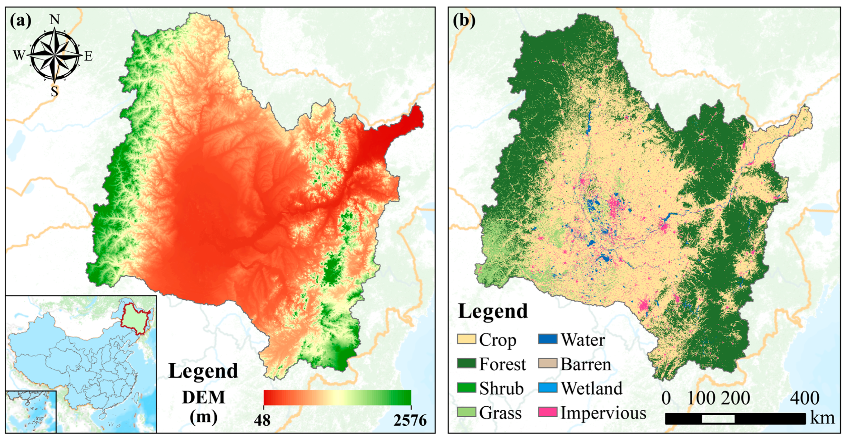
Figure 1. Location (a) and land-covers types (b) of the Songhua River Basin.
Agronomy 15 02486 g001
Figure 2. The analysis framework of the study.
Agronomy 15 02486 g002
Figure 3. Spatial distribution (a) and interannual trend (d) of GPP, spatial distribution (b) and interannual trend (e) of LOS, and spatial distribution (c) and interannual trend (f) of POS. F represents the frequency of pixel occurrence, and Fmax represents the maximum frequency of pixel occurrence.
Agronomy 15 02486 g003
Figure 4. Spatial distribution (a) and significance test (b) of the correlation between GPP and LOS; spatial distribution (c) and significance test (d) of the correlation between GPP and POS; correlation coefficient (e) and significance test (f) of the GPP-LOS correlation in different ecosystems; correlation coefficient (g) and significance test (h) of the GPP-POS correlation in different ecosystems.
Agronomy 15 02486 g004
Figure 5. Bar chart of average absolute SHAP values for GPP drivers in cropland (a), grassland (b), and forest (c); bee swarm plots of GPP drivers in cropland (d), grassland (e), and forest (f). Each point corresponds to a grid value. The y-axis in the feature ranking represents the significance of influencing factors, indicating their importance. The x-axis denotes the SHAP value, a standardized index that quantifies factor influence within the model. Additionally, the color bar in each row provides detailed information on how individual influencing factors impact phenology; yellow (purple) dots indicate higher (lower) values of these factors.
Agronomy 15 02486 g005
Figure 6. SHAP dependence plots (ac) of LOS against Pre, SHAP dependence plots (df) of POS against Pre, SHAP interaction plots (gi) of LOS and Pre, and SHAP interaction plots (jl) of POS and Pre for GPP across cropland, grassland, and forest.
Agronomy 15 02486 g006
Figure 7. SHAP dependence plots of LOS (ac) and POS (df) versus elevation, and SHAP interaction plots of LOS (gi) and POS (jl) with elevation for GPP across cropland, grassland, and forest ecosystems.
Agronomy 15 02486 g007
Figure 8. SHAP main effects of LOS (ac) and POS (df) on GPP, and SHAP dependence (gi) and interaction (jl) between LOS and POS across cropland, grassland, and forest ecosystems. Blue dots in panels (af) indicate the SHAP main effect values of individual samples, representing each sample’s contribution to the model output.
Agronomy 15 02486 g008
Table 1. Data sources and description.
DataSourcesData Description
Land use and land cover
(LULC)
The 30 m annual land cover datasets and its dynamics in China from 1985 to 2022.
(https://zenodo.org/records/8176941, accessed on 15 May 2025)
Grid, 30 m × 30 m
Elevation (Ele)Geospatial Data Cloud (China) (https://www.gscloud.cn/, accessed on 15 May 2025)Grid, 30 m × 30 m
Gross primary productivity
(GPP)
United States Geological Survey (USGS) website
(https://lpdaac.usgs.gov/product_search/?view=list, accessed on 15 May 2025)
Grid, 500 m × 500 m
Temperature (Tem)1 km monthly temperature dataset for China (1901–2022) (https://zenodo.org/records/3185722, accessed on 15 May 2025)Grid, 1 km × 1 km
Precipitation (Pre)1 km monthly precipitation dataset for China (1901–2022) (https://zenodo.org/records/3185722, accessed on 15 May 2025)Grid, 1 km × 1 km
Vegetation phenologyMODIS/Terra + Aqua Land Cover Dynamics Yearly L3 Global 500 m SIN Grid
(https://lpdaac.usgs.gov/products/mcd12q2v061, accessed on 15 May 2025)
Grid, 500 m × 500 m
Table 2. Summary of key drivers influencing GPP across different ecosystems, ranked by their importance based on mean absolute SHAP values.
EcosystemPrimary Driving FactorSecondary Driving FactorsKey Interaction (from SHAP Interaction Plots)
CroplandPreLOS > EleStrong positive interaction between LOS and Pre. GPP promotion peaks when LOS > 120 days.
GrasslandTemPre > EleWeaker phenological interactions. Tem and Ele consistently exhibit positive contributions to GPP.
ForestLOSPre > POSDominant positive effect of LOS. The LOS-POS interaction is complex, with high GPP occurring under contrasting conditions (i.e., high LOS/low POS or low LOS/high POS).
Note: The symbol > denotes more important than.
Table 3. Detection statistics of the q value of influencing factors across different ecosystem.
FactorsLOSPOSPreTemEle
Cropland0.240.140.370.180.15
Grassland0.170.180.070.540.33
Forest0.520.260.450.320.03
Disclaimer/Publisher’s Note: The statements, opinions and data contained in all publications are solely those of the individual author(s) and contributor(s) and not of MDPI and/or the editor(s). MDPI and/or the editor(s) disclaim responsibility for any injury to people or property resulting from any ideas, methods, instructions or products referred to in the content.