1. Introduction
Soil salinization has become a significant environmental problem facing the world today [
1], as salinization stress is one of the main bottlenecks in reducing crop yield and quality, as well as restricting sustainable agricultural development.
Arachis hypogaea L., commonly referred to as peanut or groundnut, is an herbaceous plant that belongs to the Fabaceae family. As an important crop type, peanuts are playing a more and more important role in people’s diets because their seeds are rich in dietary fiber, protein, vitamins, and bioactive compounds [
2], and they have been widely cultivated and consumed worldwide [
3]. In addition, peanut also has a certain salt tolerance [
4]. Therefore, the large-scale reclamation and effective utilization of saline land for peanut cultivation and the screening of saline-tolerant and high-quality peanut varieties to improve yield through research have great significance for promoting the agricultural development of saline areas, increasing farmers’ income as well as ensuring food security.
However, relatively few studies have been reported on the identification screening and evaluation of peanut varieties tolerant to salinity stress. Traditional methods for salinity stress tolerance assessment mainly rely on surveys, experiments, and statistical analyses by scientific and technical personnel. For example, Singh et al. [
5] conducted a field screening of 210 high-yielding peanut germplasm, which are identified based on plant mortality, seed yield, and nutrient uptake. Li et al. [
6] used 17 peanut varieties (lines) as materials and utilized hydroponics to determine the germination rate during the emergence period under different salt concentrations. Huang et al. [
7] cloned the
AhACO gene and functionally found that
AhACO1 and
AhACO2 significantly improved salt tolerance in transgenic peanuts. Zhao et al. [
8] found that the overexpression of
AhbHLH121 improved salt resistance, whereas silencing
AhbHLH121 resulted in the inverse correlation. The above methods involve observations and studies of the physiology, morphology [
9], and genetics of the plants [
10]. However, although the traditional method can screen out high-quality varieties to a certain extent, it is limited by time, energy, and cost.
In response to the limitations mentioned above, researchers have begun to explore an efficient and inexpensive way. With the rapid development of artificial intelligence, the utilization of deep learning combined with RGB images for plant stress identification has become a popular research direction nowadays. Esgario et al. [
11] used deep learning combined with images to estimate the severity of coffee biological stress. Chandel et al. [
12] used a deep learning model for the water stress identification of corn, okra, and soybean crops. Goyal et al. [
13] used five convolutional neural network (CNN) architectures for drought stress identification in maize images. The above studies have achieved some results in crop stress recognition by using convolutional neural networks to extract features such as color and texture in images. However, since RGB images can only provide limited visual information, they have limitations in characterizing plant responses to stress. Therefore, there exists an urgent need to find a more accurate method.
Hyperspectral (HS) imaging is an effective method for responding to information on phytochromes [
14,
15], cellular structure [
16,
17], and tissue composition [
18,
19,
20]. However, it is difficult to accurately reflect the crop growth status in real time with only one kind of data. Research has shown that the combination of canopy spectrum, structure, and temperature information in different sensor systems is conducive to improving the inversion accuracy of crop parameters. Wang et al. [
21] used data collected by HS and LIDAR to estimate the above-ground biomass of maize. Maimaitijiang et al. [
22] combined canopy spectrum information with a crop volume model. The accuracy of soybean biomass estimation was significantly improved. Zhang et al. [
23] used multi-spectral cameras, infrared cameras, and RGB cameras to analyze wheat above-ground biomass and related parameters, effectively improving the accuracy and stability of the above-ground biomass estimation model. Multimodal learning has significant advantages over single-modal learning in that it can integrate information from different data sources to provide richer features. This diversity of information enhances the robustness of the model, allowing it to maintain good performance even when a mode is missing or affected by noise. By fusing features from different modes, the model can learn more complex representations, further improving task performance.
Multimodal data have rich information content, which can be combined with deep learning techniques to better extract features. Currently, some scholars have also carried out related research; for example, Mao et al. [
24] used an unmanned aerial vehicle carrying multispectral and thermal infrared sensors to acquire multimodal data and constructed a deep learning model to assess frostbite stress in tea trees. Quan et al. [
25] constructed a deep learning model for multimodal data to predict a comprehensive competition index based on maize phenotypes. Therefore, the utilization of multimodal information for plant stress assessment is gradually becoming a new research direction.
However, this research has the following disadvantages: (1) it requires complex preprocessing using specialized software when using multimodal information; (2) the model uses the default network structure or hyperparameters, which leads to a low interpretability of the model; (3) plant-scale spectral information collected outdoors is easily affected by light, and if only point predictions are used, the prediction uncertainty may be large, which can lead to misjudgments during assessment. Therefore, it is urgent that we find an excellent method suitable for use in the assessment of peanut varieties tolerant to saline–alkali stress.
To the best of our knowledge, there has been no published research on the evaluation method of peanut saline–alkali stress tolerance based on deep learning combined with multimodal information. To rapidly identify peanut varieties that are tolerant to saline–alkali stress, this study collected the spectral information of peanut plants following normal field management, combined with deep learning and plant biological indicators. The Bayesian Optimization–Multimodal Feature Fusion Network (BO-MFFNet), which is based on Bayesian optimization and multi-modal information, was constructed to predict peanut varieties tolerant to salt and alkali stress. This model provides a method with low cost, high efficiency, high accuracy, and good stability for peanut breeding researchers to identify peanut varieties that are resistant to salt and alkali stress. The main contributions of this research are summarized as follows:
- (1)
A deep learning predictive network named Bayesian Optimization–Multimodal Feature Fusion Network (BO-MFFNet) is constructed to extract and fuse multimodal features, and its network structure and hyperparameters are optimized by the Bayesian optimization (BO) algorithm.
- (2)
An optimized Gaussian process regression (GPR) algorithm is introduced for uncertainty estimation to reduce the influence of frequent changes in outdoor light on point prediction.
- (3)
A comprehensive evaluation index is constructed for evaluating the degree of saline–alkali stress of peanut plants based on unsupervised learning.
- (4)
A non-destructive prediction method based on multimodal information fusion is proposed to judge the saline–alkali stress tolerance ability of peanut plants.
2. Materials and Methods
2.1. Dataset Acquisition
Five varieties of peanuts (Qingdao Agricultural University, Qingdao, China) are used in this research, namely Huayu25 (HY25), Yuhua31 (YH31), Yuhua32 (YH32), Yuhua33 (YH33), and Yuhua164 (YH164). The peanuts are planted in the saline and alkaline experimental fields of Qingdao Agricultural University, one located in Maotuo Village, Lijin County, Dongying City, Shandong Province, China (37°83′ N, 118°49′ E), with an average annual temperature of 12.8 °C, a frost-free period of 206 d, average annual precipitation of 556 mm, average annual evaporation of 1755 mm, soil with a pH of 8.8, a soil salinity of 0.864% [
26], and an electrical conductivity of approximately 7.86 dS/m; the other one is located in the Yellow River Delta Agricultural High-tech Industrial Demonstration Zone (37°19′ N, 118°39′ E), with an average annual temperature of 13.3 °C, a frost-free period of 206 d, average annual precipitation of 537 mm, average annual evapotranspiration of 1885 mm, soil with a pH of 7.45, a soil salinity of 0.551%, and an electrical conductivity of approximately 4.92 dS/m. An image of the site is shown in
Figure 1. Peanut planting and management are as follows: row height 10 cm, row width 112 cm, one-row double sowing, single-seed sowing. A drip irrigation technique was used to water peanuts for a period of 4 days.
To more comprehensively explore the changes in peanuts under saline–alkali stress in the field, we collected the spectral reflectance, RGB image, and photosynthetic index of peanut plants at three growth stages [
27] of full pod (R4), beginning seed (R5) and full seed (R6) in Maotuo village (MT) and Nonggao area (NG).
The spectral acquisition equipment is an Optosky ATP9100 (Optosk Technology Co., LTD., Xiamen, China) portable ground spectrometer, which has a spectral acquisition range of 300–1100 nm. The data collected are automatically interpolated on the device at 3 nm intervals of 1 nm. Measurements are taken from 10:00 to 14:00 on sunny days. To reduce the impact on soil, the spectrometer probe is 0.5 m away from the plant canopy, and the regions of interest collected are about 0.18 m
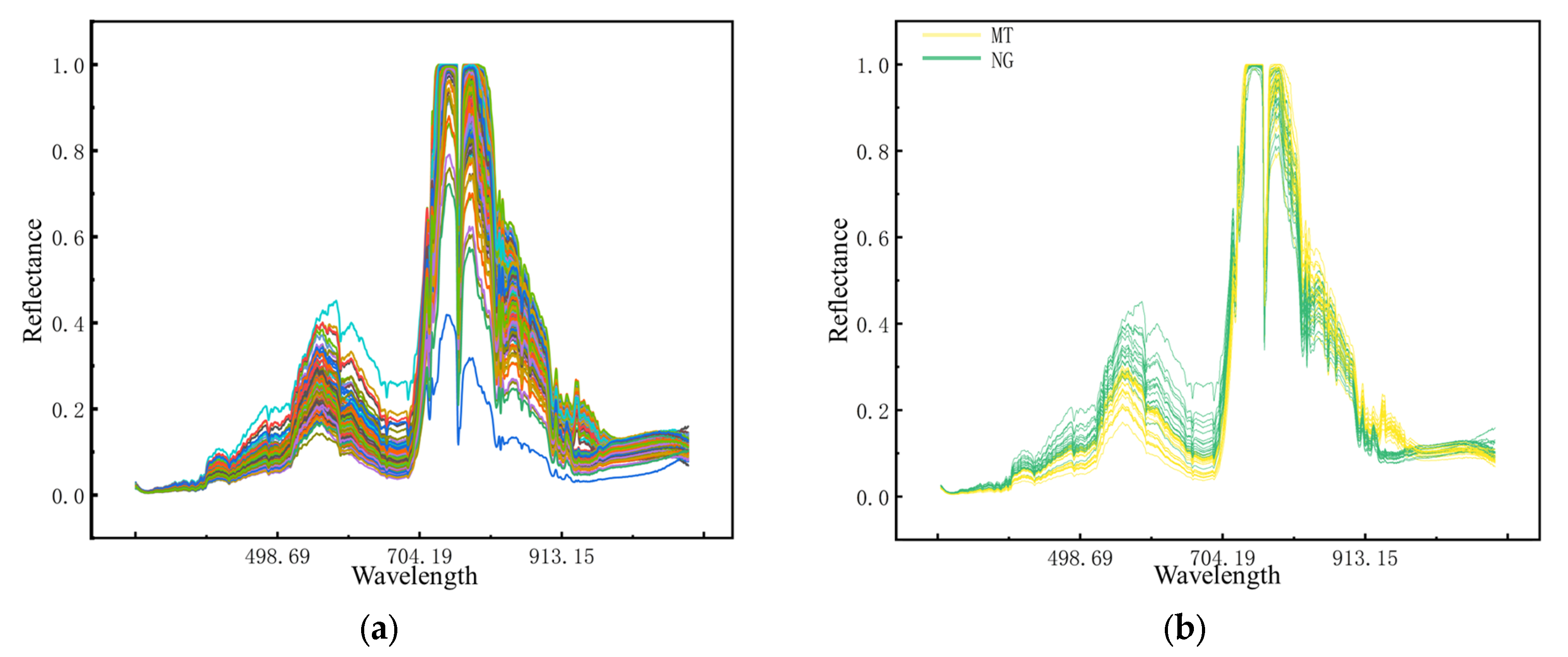
2. RGB image pixels are 480 × 640. Before each measurement, calibrate using a whiteboard. The original spectral curve of random samples in the R5 period is shown in
Figure 2. As can be seen from
Figure 2b, when peanuts are subjected to saline–alkali stress, the spectral reflectance of the peanut canopy changed significantly in the range of 520–700 nm and 930–970 nm. It has been shown that random noise in HS data can be reduced by spectral preprocessing [
28]. In this research, Savitzky–Golay (SG) smoothing is applied to raw spectral reflectance data to further reduce the effects of noise.
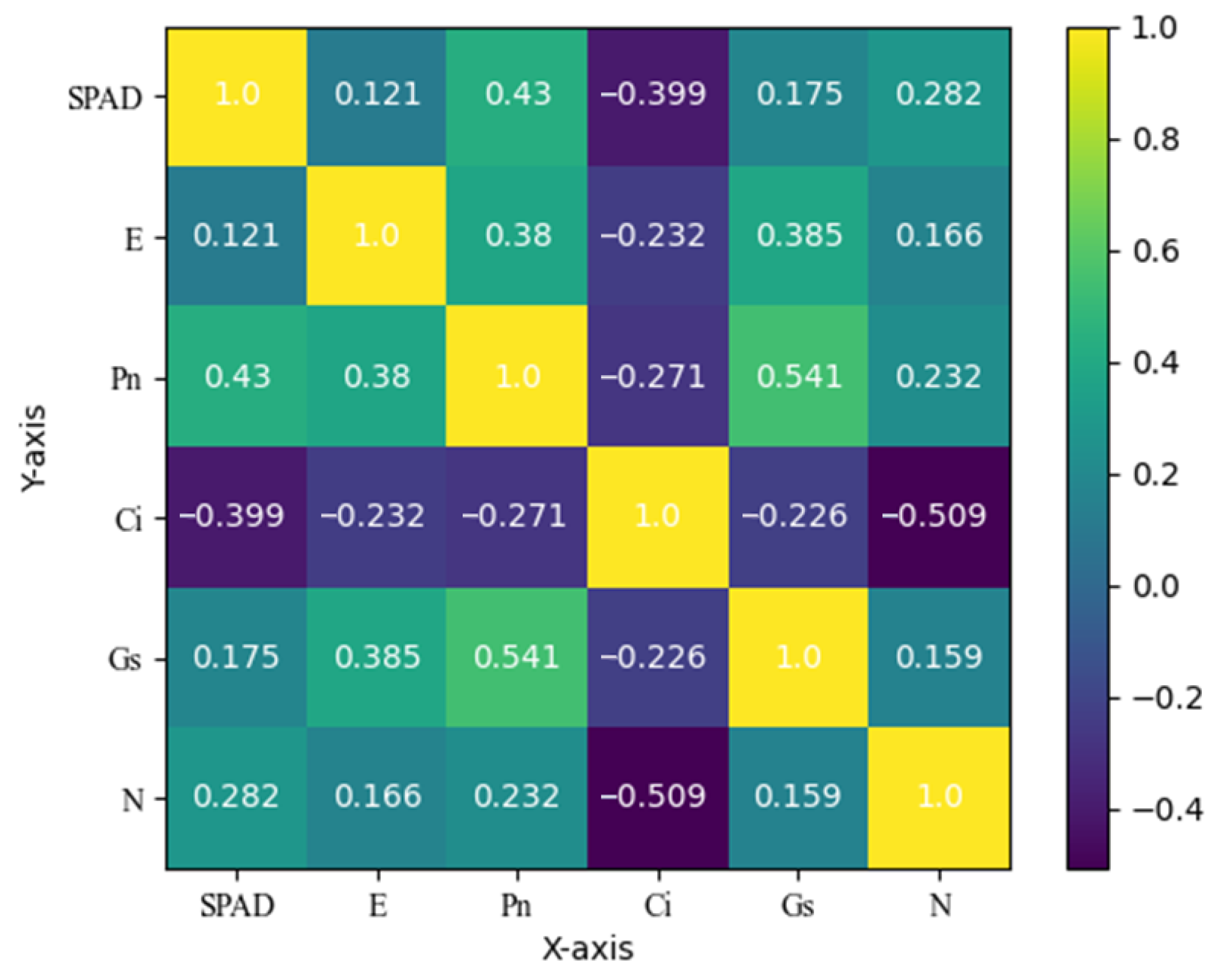
Measurements of photosynthetic parameters included chlorophyll (SPAD), leaf photosynthetic rate (Pn), stomatal conductance (Gs), intercellular CO2 concentration (Ci), transpiration rate (E), and leaf nitrogen content (N). The SPAD and N values are measured by using a portable plant nutrient meter (Zhejiang Top Cloud-Agri Technology Co., Ltd., Zhejiang, China). Other parameters are measured by using the LI-6800 Portable Photosynthesis Measurement System (Beijing LI-COR Co., Ltd., Beijing, China). The measurement times are from 10:00 to 12:00 and 14:00 to 16:00 on sunny days, and the sunny leaves in the spectral region of interest are selected for measurement under natural light source conditions. A total of 1000 peanut plant samples are collected in this research, and 30 samples are collected from each site at each growth stage. Each sample includes one HS data point, one image data point, and six photosynthetic data points.
2.2. Construction of Comprehensive Index of Saline–Alkali Stress
The principal component analysis (PCA) has significant advantages in analyzing complex datasets where labeled results cannot be obtained. PCA excels at reducing the dimensionality of the data while preserving the underlying variance, enabling the identification of underlying patterns that may not be immediately apparent. In this research, to comprehensively evaluate the saline–alkali stress of peanut plants, a saline–alkali stress score (SASS) is constructed based on the potential relationship between the variables obtained by PCA.
Specifically, first, six photosynthetic indexes were selected to reflect plant response to saline–alkali stress. To ensure comparability among different indicators, Z-Score standardization is performed. Then, dimensionality reduction is performed using principal component analysis to transform the original indicators into fewer dimensions while retaining most of the variability of the data. The principal component loading matrix is calculated, as shown in
Table 1.
It can be observed from
Table 1 that the principal components Comp1 and Comp3 have large load values on Pn, which can be regarded as the principal components reflecting the comprehensive level of saline–alkali stress in peanut plants. The principal component Comp2 has a large load value on E, which can be regarded as the principal component reflecting the comprehensive level of salt and alkali stress in peanut plants.
Finally, according to the proportion of the variance contribution rate of each principal component and the cumulative variance contribution rate of the extracted principal component, the principal component score is weighted and summed to obtain
SASS. The formula for calculating the
SASS value is:
where
X1 stands for SPAD,
X2 stands for E,
X3 stands for Pn,
X4 stands for Ci,
X5 stands for Gs, and
X6 stands for N.
The formula for the SASS value is obtained through the selection of photosynthetic metrics, PCA, and calculation of the composite score coefficients, which are used for the comprehensive assessment of peanut plants under saline–alkali stress. The formula obtained the contribution degree of each index through principal component analysis, and the contribution degree is used as the coefficient to evaluate the stress degree of plants more comprehensively.
2.3. Proposed BO-MFFNet Model
This research proposes BO-MFFNet, which is a fusion of CNN and recurrent neural network (RNN) for processing multimodal data. First, a feature extraction network is constructed to extract the features of RGB data. Then, the Bidirectional Gated Recurrent Unit (BiGRU) network is selected to extract the features of HS data. Finally, the two features are fused and the improved GPR algorithm is used for the prediction of SASS. In addition, to enhance the interpretability of the neural network and to obtain the optimal model as well as to minimize the consumption of computational resources, the network structure and hyperparameters are designed in this research based on the Bayesian optimization algorithm.
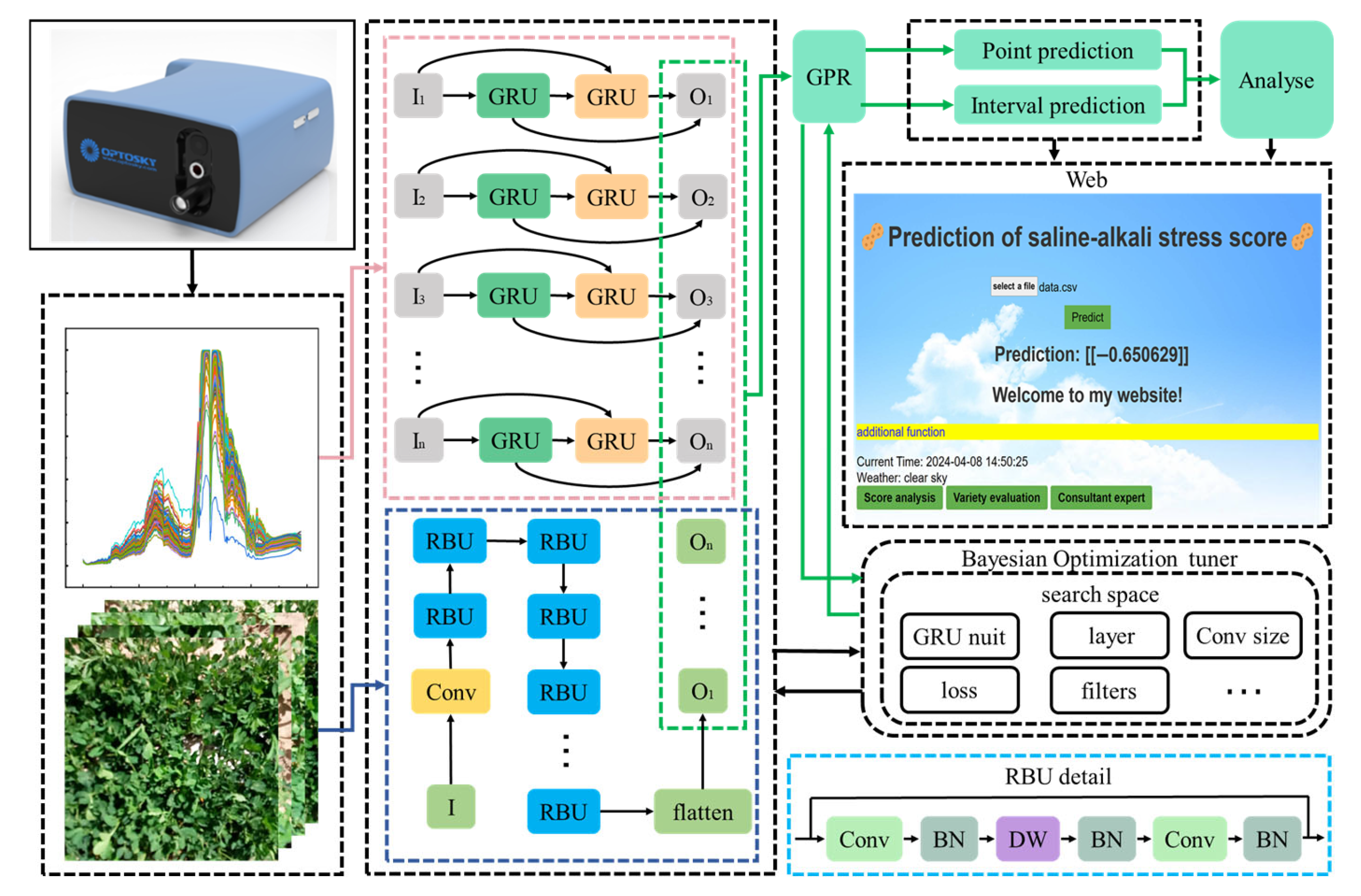
The model gives full take the advantages of CNN in spatial feature extraction, RNN in sequential data mining, and GPR which can provide an estimate of the uncertainty of the prediction. The overall schematic of the model is shown in
Figure 3.
As shown in
Figure 3, HS data features are extracted by the Bidirectional Gate Recurrent Unit (BiGRU), and RGB data features are extracted by the Residual Building Unit (RBU). The set structure of the network and the hyperparameters of the training are designed by the BO algorithm. Finally, the features are input to GPR for the point prediction and interval prediction of
SASS, where the BO algorithm searches for the following hyperparameters: the number of GRU modules, the number of RBU modules, the size of the convolution kernel, the number of channels of the convolution kernel, the loss function, the learning rate, and the optimizer.
2.3.1. Feature Fusion Network Based on Multimodal Information
To fully explore the features between different modalities and effectively fuse these features, a multimodal information feature extraction network is constructed in this research. First, this paper uses CNN to build an image feature extraction network. Among them, the structure of a single feature extraction module is shown as the RBU module in
Figure 3. The main branch increases the number of feature channels through a 1 × 1 convolutional layer, then uses depth-separable convolution for feature extraction, and finally reduces the number of channels through 1 × 1 convolutional layer to improve the performance and efficiency of the lightweight convolutional neural network. The branch paths are directly connected to the output of the main branch through jump connections. This design significantly reduces the amount of computation and model size while maintaining accuracy, which is ideal for real-time image processing tasks on mobile devices with limited computational resources.
Then, this paper uses the BiGRU model as a sequence data feature extraction network. Gated Recurrent Unit (GRU) is a gated recurrent neural network unit whose structure includes an update gate, reset gate, and new candidate states. The GRU model can grasp the important features of the HS data through the reset gate and the update gate. The following is the computational procedure of the GRU:
where
is the current moment input information, and
is the hidden state of the previous moment, which contains the data information of the previous node.
is the hidden state passed to the next time.
is the candidate’s hidden state.
is the reset gate,
is the update gate, and
is a sigmoid function. The tanh function can change the data into values in the range of [−1, 1].
,
, and
are the weight of the GRU.
The BiGRU model is a recurrent neural network consisting of several independent GRUs. One group of GRUs process data in the forward direction according to the time series, and another group of GRUs process data in the reverse direction according to the time series. The capture of bidirectional dependencies improves the model’s ability to understand sequence data, while the complex model structure allows it to adapt to more complex sequence patterns.
Finally, the features extracted by the two neural networks are fused and spliced into a one-dimensional sequence containing both image features and spectral features, and this sequence of features is input to the GPR model for prediction.
2.3.2. Interval Prediction and Uncertainty Estimation Based on Improved GPR
To evaluate the reliability of the prediction results, GPR is selected and used as the prediction layer in this research. The GPR has three main steps. First, select the appropriate kernel function and define the initial hyperparameters based on the subjective prior knowledge; then, use the probability distribution to generate the prior model and train it, find the optimal hyperparameters through the training samples; and finally, predict the test samples and give the mean and variance of the estimation results.
The Gaussian process is defined as a collection of random variables
, where any point obeys a joint Gaussian distribution. These variables are determined by the mean
and kernel functions
, as shown in Equation (3).
where
x is the input vector,
is the center of the kernel function.
The kernel function is expressed as the central moments of the random output variables corresponding to any two random input variables in the space and can be used to measure the degree to which the training set is similar or related to the test set.
The Gaussian process (
GP) can be expressed as follows:
The actual data usually contains some noise, so for the regression model, the GPR model can be obtained by adding the noise
to the observed target data
y:
where
x is the input vector,
f is the function value, and
y is the noise-contaminated observation.
The prior distribution of the observation
y can be obtained as:
and the joint prior distribution of observations
y and predicted values is:
where
is the nth-order symmetric positive definite covariance matrix and
is the covariance matrix between the test points
and the input
X of the training set.
From this, the posterior distribution of the predicted values can be calculated as:
where
is the estimate of
, and
is the covariance matrix of the test sample.
2.3.3. Hyperparameter Optimization
To design a cost-effective network structure, improve the interpretability of the model, and select the optimal hyperparameters, the BO algorithm is selected to optimize the model. BO algorithm is an efficient, robust, interpretable, and adaptive optimization algorithm, which is suitable for expensive, noisy, or uncertain problems, and provides interpretability and flexibility for the optimization process. By establishing the probabilistic model of the objective function and Bayesian inference, the BO algorithm can intelligently select parameter configuration and find a better solution in relatively few iterations. The process of Bayesian optimization used in this research is as follows: Firstly, the dataset D is initialized and the algorithm is performed 100 times; each time, the function representation of the concrete model is calculated. Then, the collection function is used to select a set of hyperparameters, which are substituted into the network for training, and the corresponding results of the set of hyperparameters are obtained. Finally, the dataset D is updated. After 100 cycles, the optimal hyperparameter with minimum loss is obtained, and the optimal model is used for training.
By the BO algorithm, the number of GRU is 64, the number of GRU layers is 2, the optimizer is adam, and the loss function is mean_squared_error. In addition, the image feature extraction model is shown in
Table 2.
2.4. Experimental Environment and Evaluation Index
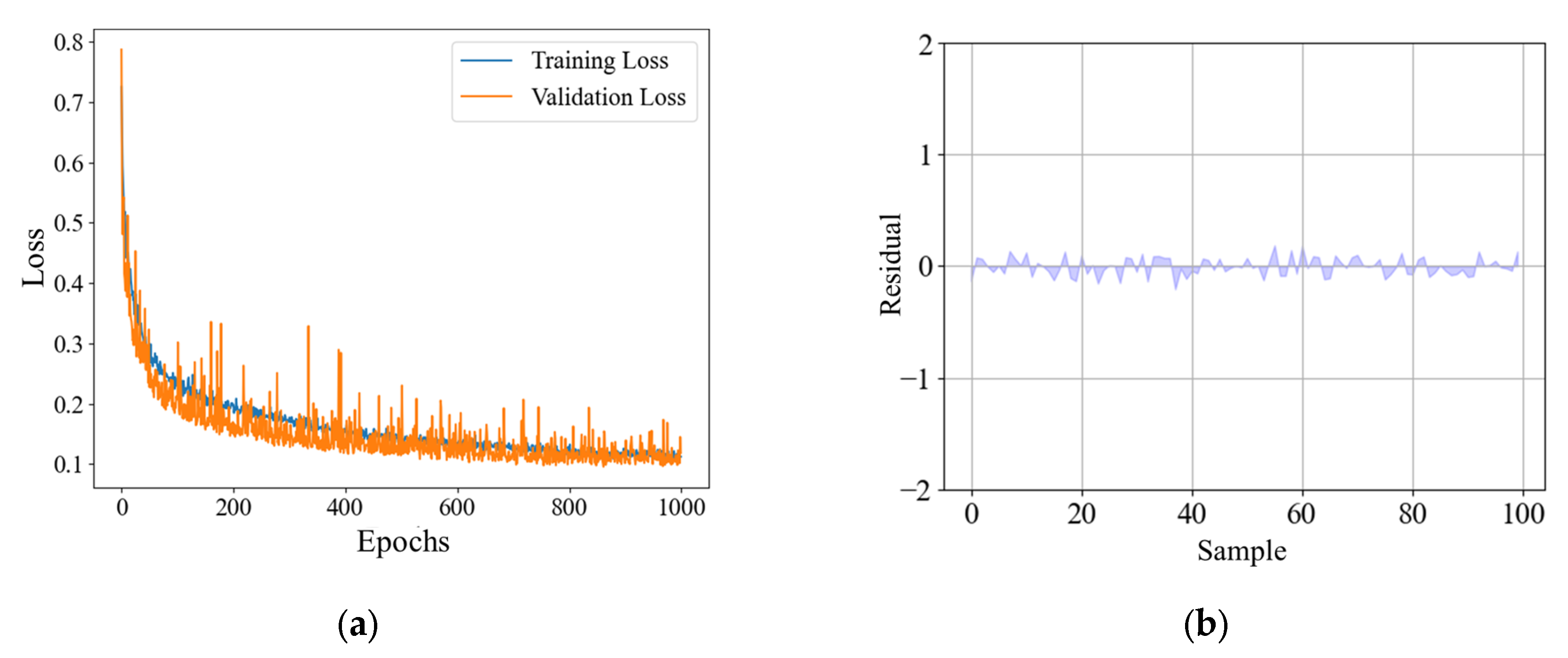
In this research, the model is trained on a Windows 10 64-bit host, and all models are based on Python language. The deep learning model is built using the TensorFlow2.10 framework. The processor is an Intel Xeon Silver 4316. The graphics card is NVIDIA A40. According to the 8:1:1 rule, the total sample is divided into datasets, and the model is trained 1000 times.
Four assessment metrics, root mean squared error (
RMSE), Mean Absolute Percentage Error (
MAPE), Coefficient of Determination
R2, and relative percentage deviation (
RPD), are selected to evaluate the performance and accuracy of the model’s model point prediction. The specific calculation is given by the following formula:
where
is the predicted value of the
ith sample,
is the true value of the
ith sample,
n is the number of samples, and
represents the standard deviation of all samples in the validation set for a particular indicator to be measured. Usually, the better the model, the larger the
R2 and
RPD, and the lower the
RMSE and
MAE.
Three interval prediction evaluation indexes, namely, Probability of Interval Coverage Probability (
PICP), Mean Width Percentage (
MWP), and Coverage Width Criterion (
CWC), are selected to evaluate the uncertainty of model prediction [
29] The specific calculation is given by the following formula:
where
N is the number of predicted samples,
yi is the
ith observation,
is the
ith prediction interval, and
is the indicator function.
is the upper bound of the
ith interval, and
is the lower bound of the
ith interval.
As the PICP increases, the true values in the prediction interval increase and the prediction uncertainty decreases. MWP represents the average percentage of the interval width concerning the observed values, which ensures the validity of the interval. The larger the MWP, the wider the interval, and the more likely that the PICP will satisfy 1. The CWC combines the PICP and the MWP, and it is a comprehensive uncertainty evaluation metric.
4. Discussion
4.1. Comprehensive Index Can Better Reflect the Degree of Plant Stress
To analyze the saline–alkali stress tolerance of different varieties, the average
SASS values of samples from different varieties are calculated in this research.
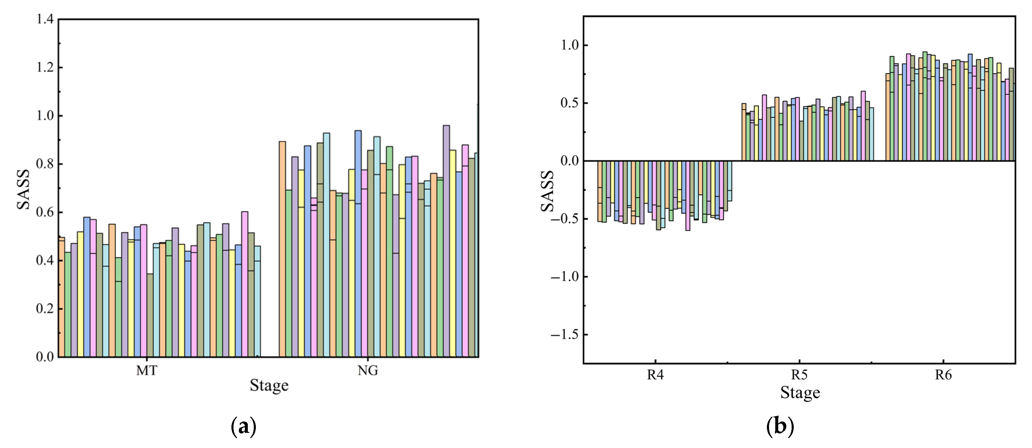
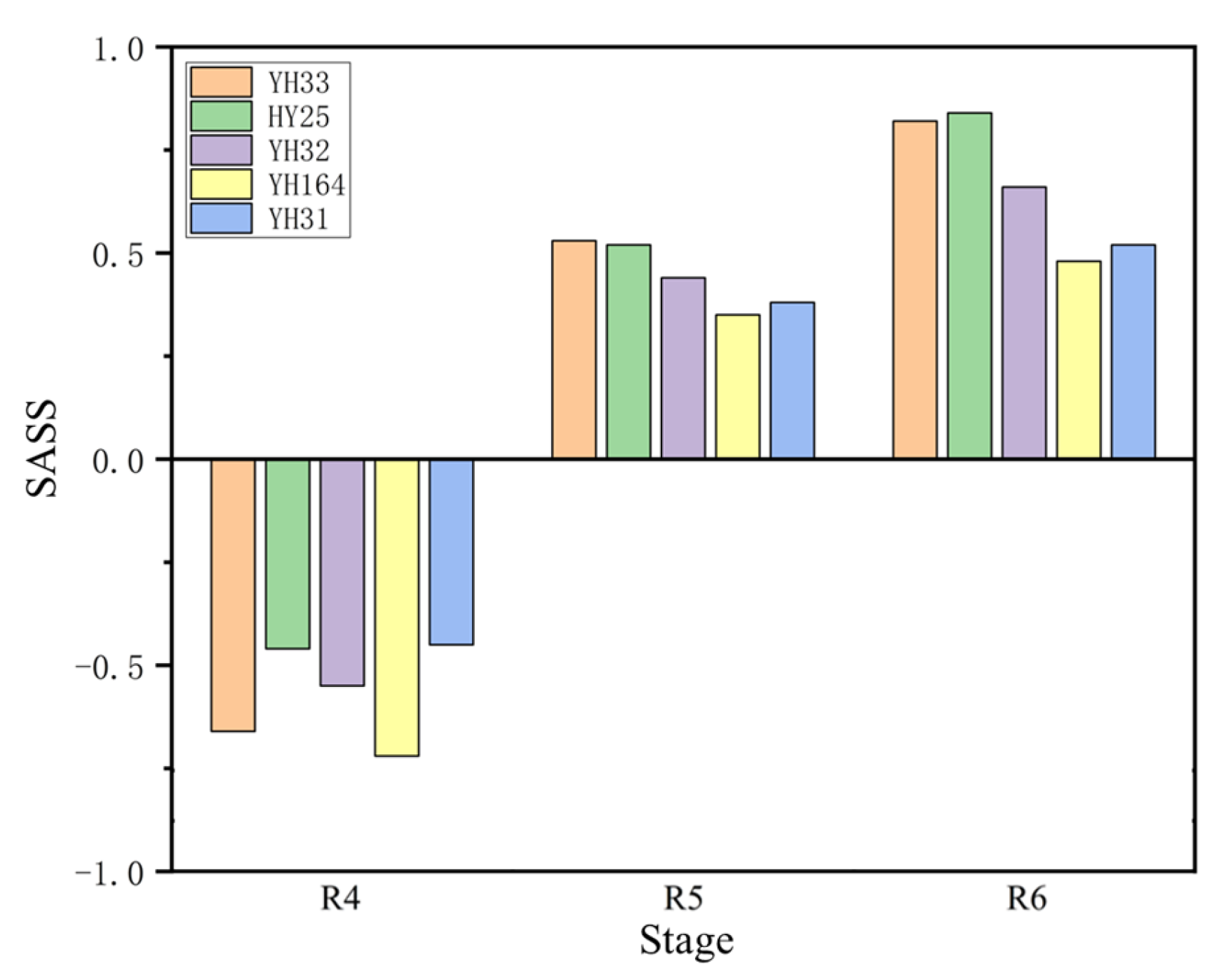
Figure 8 shows the average value of
SASS for different varieties in different stages.
As is shown in
Figure 8, different varieties of peanuts showed poor stress tolerance at the R4 stage and gradually increased stress tolerance as the plant grew. The average
SASS values for all samples of each peanut variety are as follows: YH33 (0.23), HY25 (0.30), YH32 (0.18), YH164 (0.04), and YH31 (0.15). The ranking of saline–alkali stress tolerance of the five varieties from high to low is HY25, YH31, YH33, YH32, and YH164. The members of this project adopted the traditional method, that is, the results obtained by comparing different indicators, respectively, showed that HY25 and YH31 had saline–alkali stress resistance ability; YH32 and YH33 had moderate saline–alkali stress resistance ability; and YH164 did not have saline–alkali stress resistance ability. This fully demonstrates the effectiveness of
SASS and its advantages in fine-grained classification.
Currently, the traditional method of selecting peanut varieties for tolerance to saline–alkali stress involves selecting saline soils for planting, measuring biochemical indicators at different growth stages, and evaluating them in conjunction with yield, which is a tedious process [
31]. Moreover, indirect indicators such as soil moisture or leaf appearance are often used when assessing whether a plant is under stress [
32]. However, these indicators may carry the risk of misclassification. To overcome the problem mentioned above, this research adopted a comprehensive evaluation method to evaluate the degree of saline–alkali stress of plants according to their biochemical indicators. This method can comprehensively consider the influence of many factors and improve the reliability and interpretability of the evaluation results. In addition, traditional algorithms compare different indicators, respectively, while
SASS can evaluate all indicators comprehensively and then predict
SASS quickly through hyperspectral imaging technology, which greatly saves time.
In conclusion, the method designed in this research has practical significance by integrating the analysis of photosynthetic indexes, which can provide more accurate judgments to guide the development of stress management and interventions.
4.2. Multimodal Data Can Improve the Prediction Accuracy of the Model
Saline–alkali stress can change the internal composition, color, and other agronomic traits of leaves, and then affect the light reflection intensity [
33]. In this research, it is found that the canopy spectral reflectance changes when peanut plants are subjected to saline–alkali stress. In the spectral range of about 550–600 nm, it is found that the reflectance decreases with the increase in saline–alkali stress. In the spectral range of about 920–950 nm, it is found that the reflectance increases with the increase in saline–alkali stress.
In this research, it is found through experiments that the prediction accuracy obtained by using only spectral data is low. However, this problem can be solved by fusing and supplementing data from different modalities to improve the accuracy of crop phenotype estimation [
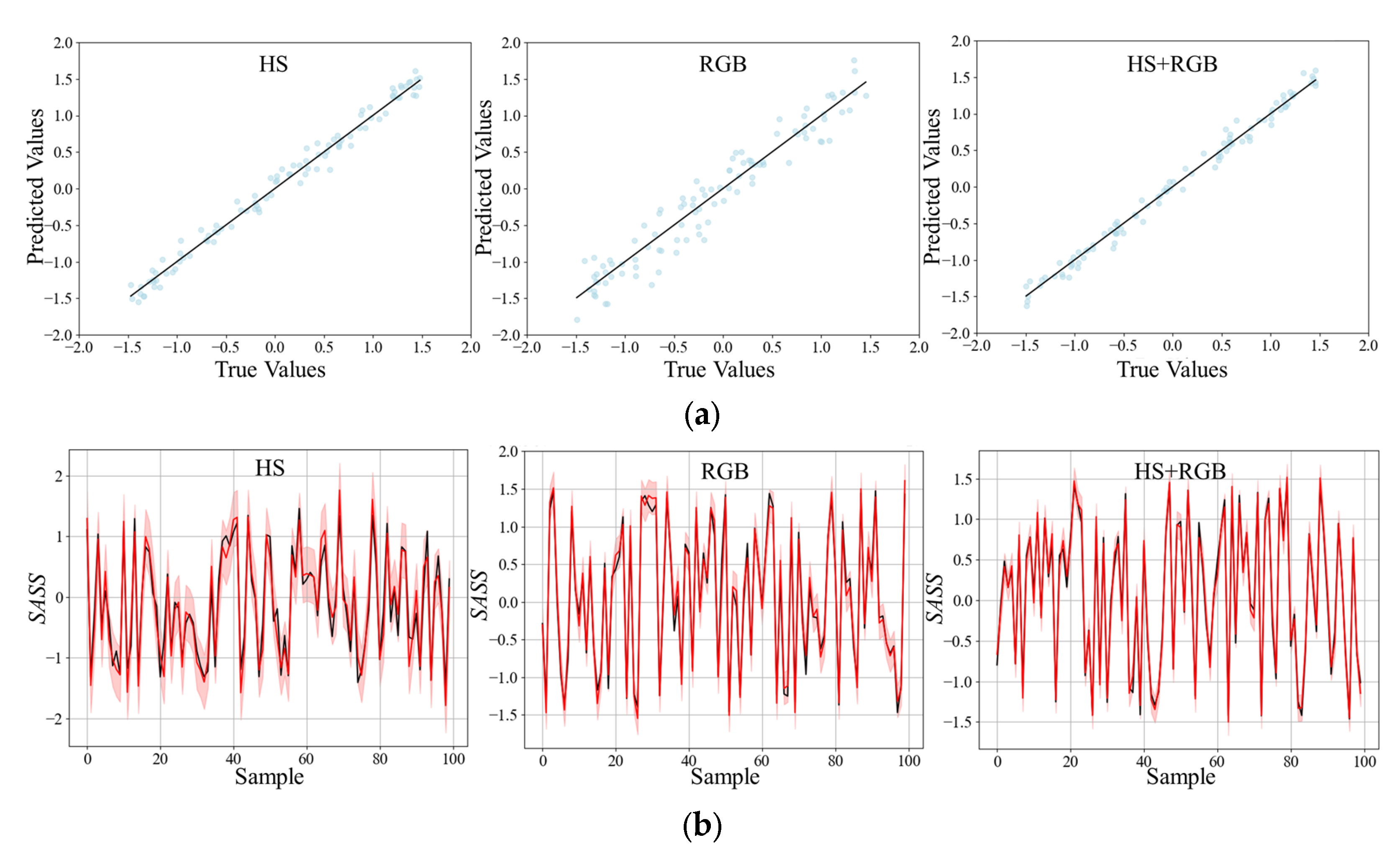
24]. RGB data are introduced in this research, which can better reflect the characteristics of objects such as color, shape, and texture. The experimental results show that the prediction effect of HS + RGB data is better than that of single-modal data. Compared with using only RGB data,
RMSE is reduced by 61.8% and
R2 is increased by 16.2%. Compared with using only HS data,
RMSE is reduced by 21.4% and
R2 is increased by 1.9%. This is because multimodal information enables the model to extract features from data of different modes, maximize the performance of the model, make use of the correlation between features, and fully learn the requirements required by the task [
34].
4.3. Interval Prediction Results Are Helpful for Decision-Making
There are many uncertainties in agricultural breeding, such as soil quality, climate change, pests, and diseases. The errors and uncertainties caused by such factors can have a significant influence on decision-making, especially in the field of agricultural breeding, where assessments require a high degree of accuracy. To our knowledge, current studies combining agriculture with prediction based on HS imaging techniques lack interval prediction methods for uncertainty assessment [
35]. Similar studies have shown that interval prediction of uncertainty evaluation is indispensable in the prediction of ginsenoside content based on HS imaging technology [
29]. Therefore, relying only on point prediction may not be reliable enough for critical decision-making [
36], especially in varietal evaluation. The GPR algorithm provides confidence intervals and interpretability of the prediction results. The GPR algorithm takes into account not only the standard deviation of the error between the predicted and actual values but also the correlation between the data and the uncertainty of the model parameters, which enables decision-makers to better assess the reliability of the prediction results and to take uncertainty into account in the decision-making process [
37].
4.4. Visual Inspection Interface
To serve breeding researchers more conveniently, a web prediction platform based on the BO-MFFNet model was constructed in this research. Predictive web pages use simple operations to complete the evaluation. First, the peanut hyperspectral data were collected using a portable ground spectrometer and uploaded to a web page, a process that takes about 10 s. By clicking the Predict button, the SASS value of the plant will be displayed on the web page, which takes about 2 s. The time required by this method is very short, and a reliable score can be obtained on the salt–alkali stress tolerance of peanut varieties. The page also has additional features such as score analysis, breed evaluation, and expert consultation available for more detailed information. In score analysis, the system interprets the meaning of the current score. Breed assessment is the assessment of a breed’s strengths and weaknesses based on its current score. Expert advice provides contact information for peanut breeders, allowing users to obtain more precise guidance.
4.5. Future Works
Future work will focus on further enhancing the comprehensive performance of the model, improving its interpretability, and optimizing its deployment. Specifically, based on the existing work, relevant indicators, such as yield, MDA, SOD, leaf area, etc., can be further collected to construct an indicator system for a more comprehensive assessment. The propagation path of the feature layer or the structure of the convolution module can be optimized to reduce the loss when the network learns the features of the seedlings, thus improving the accuracy of the prediction. The model is further extended into an APP version and deployed to mobile devices for more convenient use.
In conclusion, although the BO-MFFNet model still has some shortcomings, it provides new insights for intelligent breeding research and provides a technical reference for future research in this field.
5. Conclusions
The BO-MFFNet model proposed in this research showed good results in predicting saline–alkali stress scores of peanut plants, which can not only accurately predict the location, but also evaluate the uncertainty of the interval prediction. The experimental results show that (1) because of the single-modal model, the BO-MFFNet model has a better prediction effect on the SASS value of peanut plants, with MAE of 0.073 and R2 of 0.961. In particular, the RPD is 3.669, indicating the good fitting ability of the model. (2) After optimization by the BO algorithm, the effect of the proposed model is better than that of the conventional model. (3) The interval prediction experiment shows the low uncertainty of BO-MFFNet. (4) The proposed SASS value is superior to the traditional manual method when used to assess the saline–alkali stress tolerance of peanut varieties.
In conclusion, the combination of multimodal information, neural architecture search, and GPR interval prediction has achieved good results in the evaluation of saline–alkali stress tolerance of peanut varieties. This research provides specific methods for the efficient and reliable evaluation of abiotic stress in other crops.


