Using AI to Empower Norwegian Agriculture: Attention-Based Multiple-Instance Learning Implementation

Abstract

Agricultural development is one of the most essential needs worldwide. In Norway, the primary foundation of grain production is based on geological and biological features. Existing research is limited to regional-scale yield predictions using artificial intelligence (AI) models, which provide a holistic overview of crop growth. In this paper, the authors propose detecting several field-scale crop types and use this analysis to predict yield production early in the growing season. In this study, the authors utilise a multi-temporal satellite image, meteorological, geographical, and grain production data corpus. The authors extract relevant vegetation indices from satellite images. Furthermore, the authors use field-area-specific features to build a field-based crop type classification model. The proposed model, consisting of a time-distributed network and a gated recurrent unit, can efficiently classify crop types with an accuracy of 70%. In addition, the authors justified that the attention-based multiple-instance learning models could learn semi-labelled agricultural data, and thus, allow realistic early in-season predictions for farmers.

1. Introduction

In Norwegian agriculture, crop yield determinants are significantly influenced by agro-climatic conditions, precipitation consistency, soil quality, and greenhouse gas emissions [1]. Concurrently, the evolving dietary preferences of the global populace pose a formidable challenge to agriculturists in cultivating diverse, superior-quality cereals to meet individual nutritional demands [2,3]. This study introduces AI-facilitated methodologies for cereal categorisation, prognostication, and quality validation, aiming to bolster sustainable agricultural practices in Norway by equipping farmers with data-driven insights. This investigation identifies cereal varietals within Norway, intending to craft a pragmatic framework for forecasting cereal yields on Norwegian farms, thereby providing farmers with early or concurrent seasonal insights.

Emerging studies have employed remote sensing imagery and convolutional neural networks (CNNs) for regional crop yield forecasting. Researchers like Sharma et al. [4], You et al. [5], and Russello and Shan [6] have integrated temporal satellite imagery with CNNs, yielding precise crop yield forecasts. They enhanced prediction accuracy by amalgamating agricultural textual data with long short-term memory (LSTM). Engen et al. (2021) [7,8] innovated early-season crop yield forecasting, showcasing significant accuracy improvements with minimal error rates during specific growth season weeks in Norway.

Furthermore, this research delves into crop type categorisation models. Given Norway’s challenging agricultural climate, the diversity and extent of crops cultivated for consumption are restricted. Observations indicate a substantial portion of arable land is dedicated to cereal production, mainly barley, wheat, oats, and various rye species [9], diverging from studies that generalised crop types in Norway [10,11]. Efforts by Kussul et al. [12] and Ji et al. [13] have sought to transcend these limitations by using temporal satellite imagery in multi-dimensional CNNs. In contrast, Foerster et al. [14] validated the effectiveness of NDVI vegetation indices in differentiating twelve crop varieties, offering valuable insights for the author´s inquiry. By leveraging deep learning, the authors aim to refine precision agriculture in Norway, enhancing future sustainability [10].

1.1. Problem Statement and Hypotheses

Based on the aforementioned observations, this manuscript underscores the criticality of early yield forecasting within Norwegian agriculture, advocating for the utilisation of AI models capable of facilitating precise pre-harvest predictions. Drawing inspiration from the research conducted by Engen et al. in 2021 [7], it accentuates the importance of early forecasts tailored to specific agricultural zones while acknowledging the limitations associated with delayed data acquisition. The manuscript highlights the imperative of discerning crop types for accurate yield estimation, thereby necessitating exploring the diverse range of cereals cultivated within Norwegian farming landscapes. To address this, a semi-labelled dataset was compiled leveraging farmer-reported cereal information, notwithstanding the evident requirement for more detailed field-level data. This underscores the necessity for a robust cereal classification framework, presenting a novel, knowledge-driven methodology beneficial to farmers and the broader AI agricultural research community. This foundational work provides a compelling rationale for adopting this approach as the state-of-the-art methodology for the present research endeavour in this manuscript. To further delineate the research problem, the authors articulate five hypotheses that will be empirically tested during this study.

Hypothesis 1.

Features associated with sunlight exposure, growth temperature, ground state, and soil quality hold potential for enhancing prediction models aimed at improving grain yield forecasts.

Recent investigations using the state-of-the-art approach have demonstrated successful grain yield predictions for Norwegian farms. However, these predictions were made utilising a limited set of environmental features. Integrating additional pertinent features holds promise for refining the state-of-the-art yield prediction models in Norway. In this study, the authors intend to explore and pre-process novel features, aligning them with the same temporal resolution as the daily meteorological variables utilised in the aforementioned studies. Subsequently, the authors will reconstruct and train deep learning models comparable to those employed in the state-of-the-art approach, incorporating these newly identified features. The outcomes of this extended investigation will be detailed later in this manuscript, accompanied by a comparative analysis concerning the original grain yield prediction outcomes reported in the state-of-the-art approach. This endeavour will pave the way for exploring the second hypothesis, wherein the same model architecture will be evaluated using data spanning an additional growing season.

Hypothesis 2.

Extending the agricultural dataset to predict grain yields by incorporating an additional year of data samples is anticipated to result in improved predictive accuracy, highlighting the significance of longitudinal data collection.

Engen et al. identified the limited coverage of data across seasons as a notable constraint impacting the performance of their predictive models. Motivated by the findings of the first hypothesis, an alternative approach is proposed, focusing on including new data samples rather than introducing novel features. This methodological pivot is designed to bolster the predictive capabilities of the models and effectively tackle the challenges inherent in crop monitoring within the context of Norwegian agriculture. Consequently, agricultural and meteorological data pertinent to the 2020 season will be procured and processed in subsequent sections of this manuscript, adhering rigorously to the formatting conventions employed for features extracted from preceding seasons in the state-of-the-art investigations. Following data acquisition and pre-processing, this new dataset will be amalgamated with the preexisting dataset and subsequently leveraged to retrain the models. The ensuing evaluation will entail a comprehensive analysis of performance metrics, encompassing measures such as loss and accuracy. These findings will be expounded upon in Section 3.1, with due justification provided compared to the original findings delineated in the state-of-the-art approach.

Hypothesis 3.

Integrating satellite imagery and vegetation indices into convolutional neural networks (CNNs) offers a promising avenue for achieving precise grain classification within agricultural fields.

This research endeavour is motivated by many factors necessitating the exploration of crop classification and mapping techniques tailored to Norwegian agriculture. These include the imperative to delineate field usage and facilitate early-season yield predictions accurately. Following an exhaustive review of pertinent literature encompassing classification methodologies, feature engineering approaches, and performance benchmarks, a time-distributed CNN architecture is instantiated in the forthcoming sections. The proposed model framework incorporates raw satellite imagery alongside derived vegetation indices, leveraging the temporal dimensionality inherent in the data. Concurrently, efforts are directed towards generating ground truth class labels for fields wherever feasible to facilitate supervised learning. Subsequently, the models are trained using the amalgamated dataset. The ensuing Results and Discussion, Section 2.2.1, comprehensively presents the outcomes of the model training process, elucidating performance metrics and effectuating comparative analyses across various methodological approaches.

Hypothesis 4.

Multi-class attention-based deep multiple-instance learning (MAD-MIL) can potentially leverage entire field datasets, augmenting crop classification accuracy.

An additional rationale for undertaking crop classification endeavours stems from the need for comprehensive records detailing the crops planted and cultivated within individual fields. The extant information available, at best, yields a semi-labelled dataset. Such datasets, featuring incomplete label information, necessitate the employment of specialised methodologies inherent to semi-supervised learning, particularly within the domain of field classification in Norwegian agriculture. In the pursuit of leveraging the entirety of the dataset, a semi-supervised learning framework, specifically, multi-class attention-based deep multiple-instance learning (MAD-MIL), will be implemented in this study. This methodology endeavours to surpass the efficacy of CNN-based approaches by exploiting the inherent structure of the dataset. The ensuing section, Section 3, will explain a comparative analysis, delineating the performance disparities between the MAD-MIL approach and its CNN-based counterpart.

Hypothesis 5.

In-season early yield predictions maintain their efficacy when utilising predicted crop types based solely on the available data up to the prediction time.

The importance of in-season yield prediction, as elaborated earlier in this section, underscores the necessity within Norwegian agriculture to anticipate and project future yields. To achieve precise predictions, it is imperative for experiments to adapt by exclusively utilising information available at the time of prediction. This research endeavour aims to consolidate the insights and accomplishments obtained from preceding hypotheses into an early yield prediction framework, as outlined in Section 3. This approach’s essence lies in prognosticating each field’s crop type solely based on the earliest accessible satellite imagery, subsequently generating farm-specific masks for each predicted crop type. This methodology empowers the yield model to furnish accurate predictions early in the growth cycle. The ensuing section, Section 3, will elucidate the performance of this early yield prediction system compared to prior iterations, thereby facilitating a comparative assessment of its effectiveness.

1.2. Research Challenges and Contributions

The presented hypotheses delineate specific scenarios hitherto unexplored within the prevailing environmental and data constraints. It is the contention of the authors that these research endeavours will furnish invaluable insights and methodologies to the realms of Norwegian agriculture, food production, and AI research. Nevertheless, during experimental phases, challenges such as procuring 12-band satellite imagery for every Norwegian farm, the limited availability of data on plant growth, field specifics, and farmer activities, cloud interference in satellite imagery affecting sensor accuracy, and the heightened computational demands posed by an enlarged agricultural data corpus were encountered. In response, the research contributions encompass broadening the agricultural data corpus, improving cereal yield forecasts, substantiating the relevance of soil quality data, developing a crop classification model for early in-season yield forecasting, and appraising the current status of precision agriculture in Norway. By reflecting on these challenges and contributions, the authors introduce cutting-edge methodologies to substantiate the innovative Norwegian cereal type categorisation and yield forecasting approaches.

• Early and seasonal grain yield prediction: This research identified a pressing need for advanced in-season yield forecasting methodologies, prompting a comparative study of early prediction techniques. Employing a CNN-LSTM architecture, Sharma et al. [4] achieved minimal training and validation losses. Following Engen et al., who introduced a hybrid deep neural network that integrated various agricultural data sources, yielding a mean absolute error of 76 kg per 1000 m² and recorded error rate increases from weeks 10 to 26 and 10 to 21, respectively, this study seeks to construct an accurate early-season yield prediction framework for diverse cereal types.
• Crop type delineation and mapping: Addressing the scarcity of agriculture-specific data in Norway, Kussul et al. [12] advanced a field classification framework, demonstrating high accuracy rates for both 1D and 2D models, particularly the latter, which interprets spatial context in satellite imagery or vegetation indices. Their progress in winter wheat classification underscores the value of phenological data in remote sensing of wheat grains. Additionally, DigiFarm’s (https://digifarm.io/, (accessed on 13 April 2024)) technology, which achieves a 92% accuracy rate in delineating field boundaries and identifying crop types via satellite imagery in specific locales, is notably pertinent to this research.
• Employing vegetation indices for crop categorisation: Remote sensing techniques, which analyse the spectral composition of Earth’s surface, elucidate land, water, and vegetation features. Vegetation indices, derived from multiple spectral bands, convert reflective data into metrics that elucidate vegetation characteristics and terrestrial changes. These indices, essential in remote sensing analyses, necessitate careful selection to suit specific objectives in varied environments, especially in grain type differentiation, where variations are more nuanced [15]. This study utilises a suite of ten vegetation indices, thoughtfully chosen to optimise accuracy in cereal type categorisation.
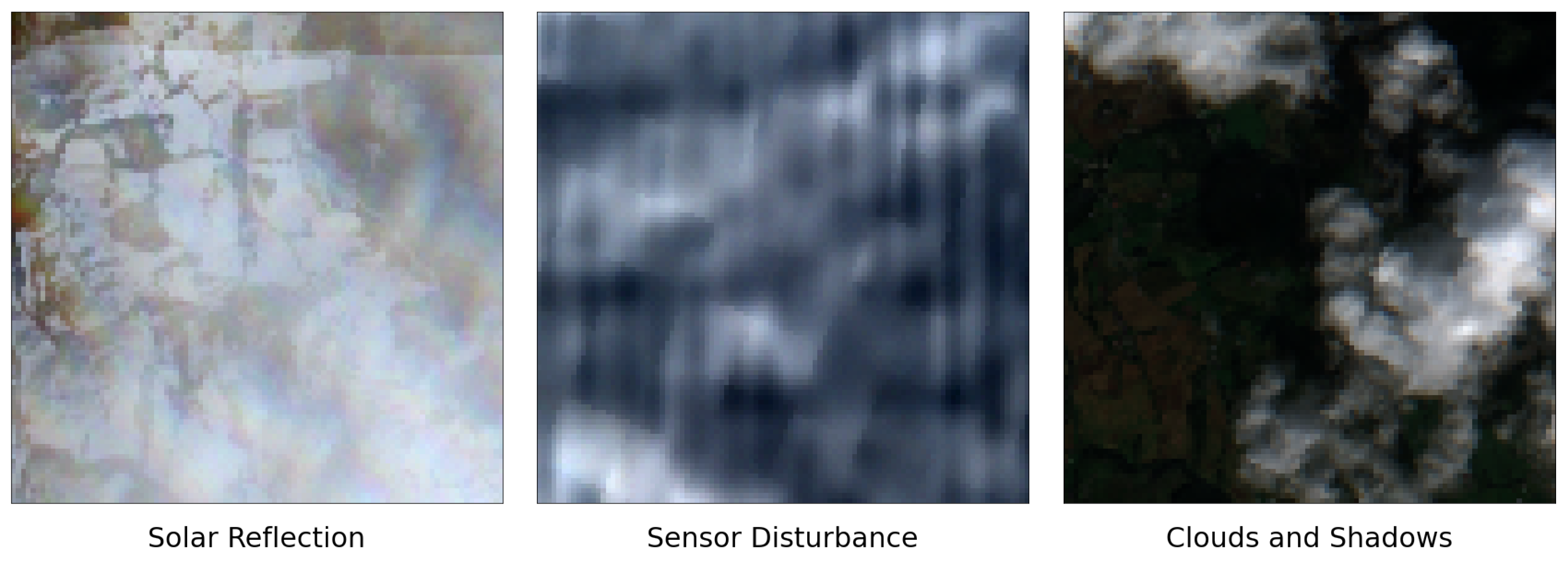
• Mitigation of cloud-induced noise in satellite imagery: The investigation acknowledges the potential of a two-step robust principal component analysis (RPCA) methodology, as outlined by Wen et al. [16], for cloud detection and mitigation in satellite images. Examples of these types of noise are visualised in Figure 1, which shows four types of noise in satellite images, solar reflection, sensor disturbance, cloud coverage, and presence of shadows, all identified at the same farm in the same year. This provides some insight into noise frequency, which can be problematic when extracting information and features from satellite images and generally results in a noisy dataset lacking essential information. Anticipating the building of such a framework to enhance analysis accuracy through noise reduction will be a focus of future work.

2. Material and Methods

This section provides a foundational background on theories and techniques pertinent to the proposed experiments, alongside an overview of antecedent experiments and research efforts relevant to AI in agriculture. A comprehensive spectrum of research endeavours and experiments will be elucidated in this section. Primarily, theories and research about agriculture, encompassing growth factors and farming activities, will be expounded upon in Section 2.1.1. Remote sensing emerges as a pivotal technique underpinning this research endeavour, given its ubiquitous application across all five research hypotheses. Section 2.1.2 furnishes a comprehensive compilation of antecedent research efforts and overarching findings in remote sensing coupled with methodologies for cloud abatement. Lastly, a foundational exposition on the principal AI techniques deployed in this research endeavour, alongside overarching work within yield prediction and crop classification, will be provided. Additionally, it will delineate comparative state-of-the-art techniques and solutions for early yield prediction and crop classification in Section 2.1.3. The research endeavours in this section will inspire the techniques and methodologies employed, serving as benchmarks for evaluating the findings when deemed pertinent. A discerning critique will be interwoven throughout the section, aimed at assessing the applicability of state-of-the-art methodologies to the methods outlined in this manuscript, thereby facilitating the execution of experiments and the evaluation of the proposed hypotheses.

2.1. Norwegian Agriculture and AI Advancements

2.1.1. Growth Factors and Farming Activities in Norwegian Agriculture

Precision agriculture constitutes a farming paradigm engineered to augment efficiency, productivity, and profitability, mirroring the objectives of this research study. Conceptually, it entails the utilisation of information technology to enhance and optimise production processes while mitigating adverse impacts on the environment and biodiversity. Often delineated as a farm-centric management strategy, precision agriculture integrates all available farm data to optimise various activities and production trajectories. Its applicability spans multiple agricultural domains, including grain production, farming, forestry, and fisheries. Nonetheless, the focus of this discourse, akin to the broader research endeavour, is directed towards grain production [18]. The variability intrinsic to grain yields can principally be bifurcated into two categories; (i) spatial variability which Signifies the divergence in soil composition, crop attributes, landscape features, and environmental conditions observed across a delineated geographical expanse [18] (p. 121); and (ii) temporal variability which denotes the fluctuation in soil properties, crop characteristics, and environmental factors discerned within a specified area at different instances of measurement [18] (p. 121).

• Status of norwegian agriculture: Norwegian agriculture demonstrates a significant reliance on the geographic positioning of farms. Contiguous regions conducive to field cultivation are primarily found along the coastline and within the Innlandet region, characterised by relatively flat terrain compared to other areas. Notably, grain production is concentrated predominantly in the low-lying areas of southern Norway, such as Innlandet. Nonetheless, a considerable portion of agriculturally viable land is designated for farming and grass production, benefiting from more favourable geographic and climatic conditions. Barley constitutes approximately half of the total grain output, with wheat and oats contributing roughly a quarter each [9]. Field preparation and sowing activities typically occur between April and May in Norway, contingent upon the duration and severity of the preceding winter and spring seasons. Spring-sown crops typically reach maturity by September, marking the commencement of the harvesting period. However, the harvest timing is subject to variables such as the sowing schedule and various temporal factors affecting the growth cycle. Autumn-sown grains are typically planted between August and September in Norway; however, these grains are beyond the scope of the present research endeavour [19].
• Meteorological factors: Optimal spring farming conditions necessitate minimal precipitation and sufficiently warm temperatures to facilitate ground thawing, enabling the use of heavy equipment for field operations such as ploughing and sowing. Dry soil conditions enhance manageability during these activities. Ideal lighting conditions for seed germination involve fluorescent cool white lights, as incandescent lights may generate excessive heat harmful to crops. Grain seeds and plants require stable temperatures and regular precipitation throughout the growing season to develop into harvestable grains. At maturity, grain plants must undergo drying to reduce moisture content for safe harvesting and storage [19,20].
  Temperature and precipitation profoundly influence farming operations and plant growth. Research by Johnson et al. (2014) [21] highlights the significant correlation between weather variables and crop yield, with a consensus favouring a favourable combination of warmth and rainfall for increased yields. Sunlight, crucial for photosynthesis and photomorphogenesis, benefits grain crops, with prolonged exposure often moderating temperature extremes. However, excessively high temperatures exceeding 30 °C, notably surpassing 45 °C, can stress or even kill most plant species [22]. Kukal and Irmak (2018) [23] emphasise the substantial impact of climate variability on crop yields, with precipitation emerging as a critical predictor across maize, sorghum, and soybean crops. These insights underscore the vital importance of temperature and precipitation in shaping crop growth and yield outcomes, informing effective yield prediction models.
• Agriculture field and soil factors: Soil texture and quality influence plant growth by dictating nutrient and water retention, water flow dynamics, and soil stability against disruptive forces. Factors such as animal activity, mechanical fieldwork, organic matter depletion, and cultivation practices can adversely impact soil properties, affecting water and oxygen capacity and promoting evaporation, thereby influencing seed and plant viability. Yield correlations are often observed with soil susceptibility to erosion by water and wind. Organic matter stabilises soil structure, enhances nutrient retention, and fosters microbial activity. Soil moisture content, accounting for up to 50% of yield variability, impacts soil temperature and nutrient uptake. Addressing soil factors such as water availability and organic matter content through fertilisation and irrigation can enhance plant productivity [18]. Field elevation and slope variations can also impact crop yields indirectly. Higher-altitude fields tend to be shallower with coarser textures, potentially impeding plant growth. Conversely, lower-altitude fields may experience colder air, hindering water accumulation and movement through the soil [18]. Foerster et al. [14] conducted crop classification and mapping, observing high temporal variability in the seasonal Normalised Difference Vegetation Index (NDVI), attributed to crop dependence on specific soil properties and water availability. These findings underscore the significance of soil characteristics in influencing crop growth and suggest that incorporating such information can refine crop classification and yield prediction models, enhancing agricultural decision-making processes.
• Farming activities: Various farming practices, such as fertilisation, irrigation, and field preparation techniques, significantly influence crop growth and yield outcomes. Farmers often utilise fertilisers and irrigation to enhance soil nutrient content and moisture levels, creating favourable conditions for plant growth. Irrigation, in particular, is crucial in mitigating the adverse effects of high temperatures and low precipitation, contributing to more stable yields amid climate variability. Additionally, organic farming practices prioritise sustainability over yield, employing natural fertilisers and crop rotation strategies to maintain soil fertility and ecosystem health. Field preparation activities, including ploughing, cultivation, and sowing, also impact crop performance by facilitating optimal seed placement and germination conditions. Studies such as that by Shah et al. [24] underscore the significance of factors like sowing date in determining yield outcomes, albeit within specific regional contexts. In summary, accounting for a comprehensive range of farming activities in yield prediction datasets is essential for accurately assessing crop growth and productivity.

2.1.2. Remote Sensing in Norwegian Agriculture

Prior to the emergence of readily accessible remote sensing technology, scholars relied upon surveys about meteorological phenomena, agricultural land conditions, and crop categorisations to facilitate the prediction and monitoring of crop yields. However, acquiring such data posed formidable challenges, frequently proving arduous and inaccessible, particularly within developing regions. The difficulties of precision agriculture, which necessitate a copious volume of samples for effective implementation, further compounded the obstacles associated with data procurement. In conjunction with their temporal dynamics, the documentation of field attributes, surface characteristics, and soil properties entailed substantial temporal and financial investments, thereby inherently constraining the process. These challenges underscore the pivotal role of remote sensing as a promising and productive modality in agricultural research [5]. Through remote sensing technologies, researchers are empowered to surmount the limitations inherent to traditional data collection methodologies, thereby facilitating the comprehensive monitoring and analysis of agricultural terrains. Remote sensing involves detecting and surveilling physical attributes within a defined area by analysing reflected radiation, typically through sensors deployed on satellites or aircraft [2]. Satellite sensor systems provide spectral, spatial, and temporal data regarding target objects like fields and farms. Spectral data encompasses insights from distinct sensor bands and visual wavelengths, while spatial data relates to geographical dimensions. Temporal data tracks evolving conditions, enabling diverse agricultural applications such as improved weed and water management, crop mapping, drought detection, and growth monitoring [25]. Remote sensing also allows for deriving numerous vegetation indices, capturing essential parameters like chlorophyll content and leaf area index [26]. Nonetheless, the effectiveness of remote sensing systems is constrained by susceptibility to atmospheric disturbances and cloud cover, necessitating noise mitigation strategies in data processing [27,28].

• Mitigation of cloud-induced noise in satellite imagery: Data acquired through remote sensing systems are vulnerable to various sources of noise, encompassing factors such as sensor orientation, atmospheric fluctuations, and phenomena such as cloud cover. Consequently, satellite imagery often contains contaminants like noise, clouds, and dead pixels, posing challenges to data integrity [12,29]. Reflective information captured by sensors can undergo distortion due to atmospheric influences, such as water droplets leading to cloud formation or optical impediments causing shadows, exacerbating the issue [30]. These artefacts significantly disrupt the usability of remote sensing data, necessitating pre-processing techniques to enhance their quality [31]. Kussul et al. [12] addressed noise and reflection issues in satellite images for land classification by employing a method involving masking out noisy regions and utilising self-organising Kohonen maps to restore missing pixel values in specific spectral bands [32]. Rooted in machine learning algorithms, this approach demonstrated potential for improving yield predictions and grain classifications in agricultural research contexts.
  Moreover, various information reconstruction methods have been devised for remote sensing images [29]. Zhang et al. [33] proposed a deep learning framework employing spatial–temporal patching to address thin and thick cloudy areas and shadows in Sentinel and Landsat images. Lin et al. [34] adopted an alternative strategy, utilising information cloning to replace cloudy regions with temporally correlated cloud-free areas from remote sensing imagery, assuming minimal land cover change over short periods. Additionally, Zhang et al. [35] developed a novel approach for reconstructing missing information in remote sensing features using a deep convolutional neural network (CNN) combined with spatial–temporal–spectral information. This framework showed promising results in mitigating cloud and noise issues, offering a feasible solution for enhancing the quality of satellite images pertinent to agricultural applications. However, applying such methodologies to satellite imagery of Norwegian farms necessitates access to suitable datasets comprising both cloudy and cloud-free spatial–temporal data, entailing substantial time investment for dataset preparation.
• Derived vegetation indices: Remote sensing systems excel in capturing and interpreting the spectral composition of radiation emitted from the Earth’s surface, facilitating insights into land, water bodies, and various vegetation features. Vegetation indices, derived from multiple remote sensing spectral bands, serve as straightforward transformations aimed at condensing reflective information into more interpretable metrics, thereby enhancing understanding of vegetation properties and terrestrial dynamics [36,37]. The origins of vegetation indices trace back to 1972, with Pearson and Miller pioneering the creation of the first two indices to discern contrasts between vegetation and ground surfaces [38]. Subsequently, over 519 unique vegetation indices have been developed, tailored to diverse purposes, applications, and environmental contexts [26]. However, not all vegetation indices are universally applicable, as demonstrated by studies indicating limitations of widely used indices like the Normalised Difference Vegetation Index (NDVI) and Enhanced Vegetation Index (EVI) in specific scenarios [39,40]. Accordingly, selecting suitable vegetation indices for particular research objectives and environmental conditions is imperative, particularly in contexts such as crop type classification, where nuances among grain types pose challenges [15].
  Fundamental studies, exemplified by Massey et al. [41], have underscored the utility of vegetation indices, notably NDVI, in crop mapping and classification endeavours. Leveraging decision tree algorithms and time-series NDVI data extracted from satellite images, Massey et al. achieved notable accuracy in crop type classification, demonstrating the efficacy of NDVI despite challenges stemming from similarities among target crop types. Ten vegetation indices were meticulously selected in this research based on theoretical foundations, practical applications, and extant literature. These indices are elucidated alongside their respective theories, applications, and formulae, sourced from Kobayashi et al. [42], Henrich et al. [26], and pertinent references. Notably, the wavelength parameters in the formulae represent ranges rather than precise values, acknowledging variations in band wavelengths across diverse remote sensing systems. This variation necessitates adaptability in selecting neighbouring band wavelengths for specific indices.
  • Enhanced Vegetation Index (EVI) distinguishes the canopy structure and vegetation growth status of crops and is calculated from the visible near-infrared. Equation (1) shows how the EVI is calculated. L is a canopy background adjustment value. $C_1$ and $C_2$ are aerosol resistance coefficients that correct aerosol influences between wavelengths of 640 and 760 nm by using a band between wavelengths of 420 and 480 nm, and G is the gain factor. These factors are used between different remote sensing systems to account for their unique reflections and atmospheric values [37].

    $$G\ast \frac{\left(780:1400\mathrm{nm}\right)-\left(640:760\mathrm{nm}\right)}{(\left(780:1400\mathrm{nm}\right)+C_1\ast \left(640:760\mathrm{nm}\right)-C_2\ast \left(420:480\mathrm{nm}\right)+L)}$$

    (1)
  • Land Surface Water Index (LSWI) distinguishes the water content in crops based on near- and shortwave infrared. These bands are sensitive to soil moisture and leaf water, making the LSWI sensitive to water. Equation (2) shows how the LSWI is calculated [39].

    $$\frac{\left(841:875\mathrm{nm}\right)-\left(1628:1652\mathrm{nm}\right)}{\left(841:875\mathrm{nm}\right)+\left(1628:1652\mathrm{nm}\right)}$$

    (2)
  • Normalised Difference Senescent Vegetation Index (NDSVI), designed by Qi et al. [43], distinguishes both water content and the growth status and is based on visible shortwave infrared, a combination of the EVI and LSWI. Equation (3) shows how the NDSVI is calculated. These wavelengths are in the water absorption regions of the spectrum and can, therefore, be combined to extract information related to senescent vegetation.

    $$\frac{1640\mathrm{nm}-(640:760\mathrm{nm})}{1640\mathrm{nm}+(640:760\mathrm{nm})}$$

    (3)
  • Normalised Difference Vegetation Index (NDVI), designed by Rouse et al. [44], measures the amount and density of green vegetation based on the near-infrared and red bands. This is useful for agriculture, as unhealthy crops reflect less near-infrared than healthy crops [45]. Equation (4) shows how the NDVI is calculated. The normalisation in the NDVI enables it to consistently measure the greenness with fewer deviations than a more straightforward ratio of the two bands [44].

    $$\frac{\left(1300:3000\mathrm{nm}\right)-\left(800:900\mathrm{nm}\right)}{\left(1300:3000\mathrm{nm}\right)+\left(800:900\mathrm{nm}\right)}$$

    (4)
  • Shortwave Infrared Water Stress Index (SIWSI), estimates the water content of crop leaves. A shortwave infrared band operates on a wavelength influenced by leaf water content, enabling SIWSI to extract information related to the water content in crops. This can identify the stress level inflicted by the water content. Equation (5) shows how the SIWSI is calculated. An index value below zero indicates that the crops have sufficient water content. In contrast, values above zero indicate that the crops are experiencing some level of water stress due to too much water [46].

    $$\frac{860\mathrm{nm}-1640\mathrm{nm}}{860\mathrm{nm}+1640\mathrm{nm}}$$

    (5)
  • Green–Red Normalised Difference Vegetation Index (GRNDVI), created by Wang et al. [47], is one of multiple vegetation indices using a combination of the red, green, and blue bands in an NDVI manner. The GRNDVI is one of the better vegetation indices for measuring leaf area index (LAI), an important feature related to crop health, growing stage, and type. Equation (6) shows the calculation for the GRNDVI.

    $$\frac{\left(780:1400\mathrm{nm}\right)-\left(\right(490:570\mathrm{nm})+(640:760\mathrm{nm}\left)\right)}{\left(780:1400\mathrm{nm}\right)+\left(490:570\mathrm{nm}\right)+\left(640:760\mathrm{nm}\right)}$$

    (6)
  • Normalised Difference Red-Edge (NDRE) is a vegetation index similar to the NDVI, which uses a ratio between the near-infrared and red-edge bands. It can extract information from remote sensing data regarding crops’ health and status, including the canopy’s greenness. Equation (7) shows the calculations for NDRE [48,49].

    $$\frac{\left(780:1400\mathrm{nm}\right)-\left(690:730\mathrm{nm}\right)}{\left(780:1400\mathrm{nm}\right)+\left(690:730\mathrm{nm}\right)}$$

    (7)
  • Structure Intensive Pigment Index 3 (SIPI3) is a function of carotenoids and chlorophyll a. Carotenoids provide information about canopy physiological status while chlorophyll includes information about plant photosynthesis. The original SIPI was designed by Penuelas et al. [50] while attempting to achieve the highest correlation between carotenoids and chlorophyll for acquiring plant physiology and phenology information. The SIPI3 is a variation of this, shown in Equation (8).

    $$\frac{800\mathrm{nm}-470\mathrm{nm}}{800\mathrm{nm}-680\mathrm{nm}}$$

    (8)
  • Photosynthetic Vigour Ratio (PVR) is a simple combination of the red and green bands, reflecting chlorophyll absorption, canopy greenness, and photosynthetic activity. Equation (9) shows the formula for the PVR [18,49].

    $$\frac{550\mathrm{nm}-650\mathrm{nm}}{550\mathrm{nm}+650\mathrm{nm}}$$

    (9)
  • Green Atmospherically Resistant Vegetation Index (GARI), created by Gitelson et al. [51], is a vegetation index resistant to atmospheric effects while also being sensitive to a range of chlorophyll-a concentrations, plant stress, and rate of photosynthesis. The GARI is as much as four times less sensitive to atmospheric effects than the NDVI while providing similar information. Equation (10) shows how the GARI is calculated.

    $$\frac{\left(780:1400\mathrm{nm}\right)-\left(\right(490:570\mathrm{nm})-(\left(420:480\mathrm{nm}\right)-\left(640:760\mathrm{nm}\right)\left)\right)}{\left(780:1400\mathrm{nm}\right)-\left(\right(490:570\mathrm{nm})+(\left(420:480\mathrm{nm}\right)-\left(640:760\mathrm{nm}\right)\left)\right)}$$

    (10)

2.1.3. AI for Norwegian Agriculture: Crop Yield Prediction

Crop yield prediction has been explored across various environments, employing diverse data types and machine learning models. Raun et al. [52] conducted a study to ascertain the feasibility of predicting winter wheat grain yields using multi-spectral seasonal features. They achieved a high correlation with yield by incorporating two Normalised Difference Vegetation Index (NDVI) measurements into an estimated yield feature, explaining 83% of yield variability. However, their approach could not capture growth changes due to environmental factors such as rain, lodging, and shattering. Nevavuor et al. [53] and You et al. [5] employed deep learning techniques for crop yield predictions. Nevavuor et al. utilised RGB bands and NDVI from multi-spectral images in a convolutional neural network (CNN) model, achieving a mean absolute percentage error (MAPE) as low as 8.8%. You et al. utilised temporal satellite images and textual features to predict soybean yields, reducing the root mean square error (RMSE) by 30%

Khaki and Wang [54] integrated genotype, soil, and weather data into a deep neural network (DNN) to predict corn yield and yield difference. Their model, trained on soil and weather data, yielded an RMSE of 11%, outperforming regression tree and least absolute shrinkage and selection operator methods. Their findings underscored the importance of soil and weather data in yield prediction, advocating for weather prediction as an essential component. Russello and Shan [6] utilised satellite images in a CNN to predict soybean yields, identifying features between February and September as most crucial for prediction. Basnyat et al. [55] investigated the optimal timing for using remote sensing to predict crop yield by analysing the correlation between the NDVI and yield across different periods. They concluded that the NDVI derived between the 10th and 30th of July was most suitable for predicting yields of spring-seeded grains, aligning with the maturity period of these crops. These findings are pertinent for evaluating the timing of early yield predictions for Norwegian farms, considering that spring-seeded grains in Norway typically mature in September.

• Crop classification and mapping: Satellite imagery has demonstrated efficacy in classifying various crop types and capturing their spectral dynamics, facilitating the detection of phenological disparities among them. However, leveraging satellite images for classification purposes presents inherent challenges [15]. For instance, Hu et al. [56] and Qui et al. [57] observed that stacking satellite images throughout the growing season often yielded redundant information. Hence, it is imperative to discern the types of features to employ and the appropriate AI architectures and techniques to utilise. Castillejo-González et al. [28] investigated the impact of transitioning from pixel-based classification (1D) to object-based classification (aggregating pixels). Their findings consistently favoured the object-based approach, indicating the superiority of 2D images over single-pixel values for grain classification. Ji et al. [13] employed multi-spectral temporal satellite images in 3D convolutional neural networks (CNNs) for crop classification. By leveraging a 3D CNN framework, they captured the temporal representation of the entire growing season, outperforming analogous 2D methods and exhibiting exceptional proficiency in identifying growth patterns and crop types. The prevalence of 3D CNN architectures in achieving superior feature extraction and representation of multi-spectral temporal data is well documented. Due to the diminished accuracy of pixel-based classification methods, Peña-Barragán et al. [58] devised an Object-Based Crop Identification and Mapping model, attaining an accuracy of 79%. Their analysis highlighted the substantial contribution of remote sensing images from the late-summer period to the classification model, followed by mid-spring and early-summer images. This disparity underscores the significance of late-growing-season images and underscores the challenge of early-season classification.
• Attention-based multiple-instance learning: In image classification research endeavours, datasets typically possess consistent labelling corresponding to their respective classes. However, this conformity is often lacking in real-world applications, as evidenced in medical imaging studies where multiple images may need more specific class labels, providing only generalised statements regarding their categorisation. Similarly, in agricultural contexts, the labelling of crops for each field needs to be completed, resulting in a semi-labelled dataset. Multiple-instance learning (MIL) has emerged as a thoroughly investigated semi-supervised learning method [59,60,61] to mitigate this challenge. MIL aims to predict the labels of bags, where bags comprise a mixture of labelled and unlabelled instances, departing from the conventional approach of classifying individual instances. In a traditional MIL framework, a single target class is specified, and bags are labelled as positive or negative depending on the presence or absence of at least one instance of the target class. Consequently, comprehensive knowledge of instance labels becomes unnecessary, thereby enhancing the suitability of MIL in scenarios with partially labelled data [60,62]. Notably, MIL models incorporate an attention mechanism that assigns an attention score to each instance within a bag, indicating its influence on bag classification. These scores are calculated using the softmax function, ensuring their collective summation to unity.
  Prior research has explored various approaches to bag classification. Cheplygina et al. [63] introduced bag dissimilarity vectors as features in the training dataset, representing each bag’s dissimilarity. Chen et al. [64] leveraged instance similarities within bags to construct a feature space, extracting crucial features for traditional supervised learning. Raykar et al. [65] investigated diverse instance-level classification techniques and feature selection methods within bags, yielding promising and competitive outcomes.
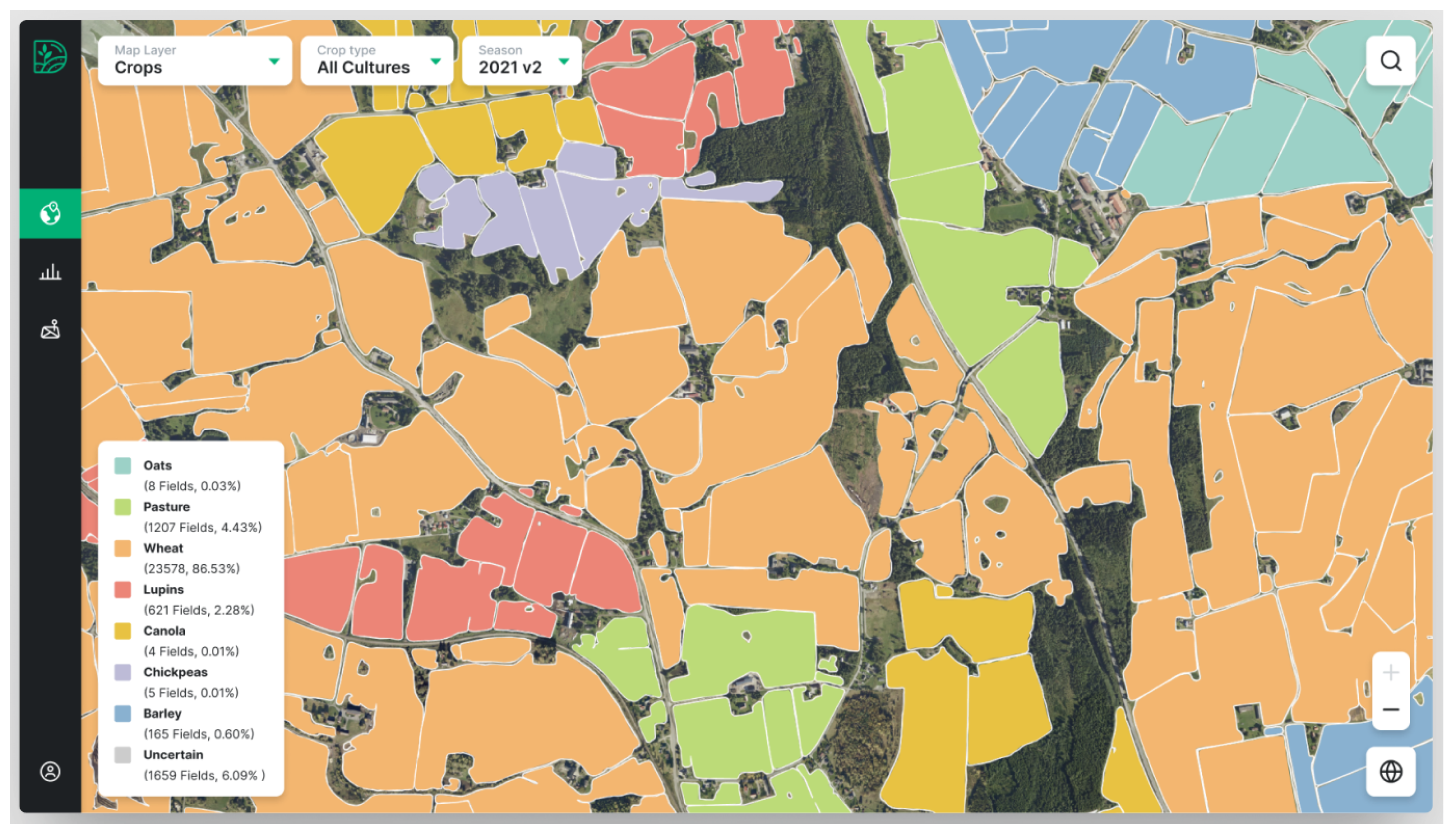
• State of the art techniques: In this section, the authors present state-of-the-art research endeavours pertinent to each hypothesis delineated earlier in this manuscript. The major focus is on identifying the most promising technique for cloud and noise removal and surveying multiple studies concerning crop classification utilising vegetation indices, thereby facilitating the selection of appropriate indices. Furthermore, the authors provide an overview of comparative state-of-the-art methodologies and solutions for early yield prediction and crop classification. The insights gleaned from these research efforts serve as a source of inspiration for the techniques and methods applied in this research study, serving as benchmarks against which to evaluate the outcomes in forthcoming sections.
  Detecting clouds in remote sensing images to create a training dataset may pose challenges for this research study. To address this requirement, Wen et al. [16] proposed a two-step robust principal component analysis (RPCA) framework designed to identify cloud regions within satellite images, removing them and restoring the affected areas. Their innovative approach obviates the need for a cloud-free satellite image dataset or any preliminary cloud detection pre-processing steps. Among the various promising cloud removal methods available, the recent work by Wen et al. [16] emerges as the most suitable technique. Given the time availability constraints, their methodology holds promise for mitigating noise in satellite images, potentially enhancing the accuracy of pertinent deep learning models.
  Sharma et al. [4] conducted an extensive investigation into the temporal dynamics of crop yield prediction, emphasising the importance of early-stage observations. Their study highlighted the critical role of satellite images in predicting crop yields from the initial months of the growing season, particularly the first month. Through systematic evaluation by replacing images from each month with noise and assessing the resulting root mean square error (RMSE), they demonstrated a significant increase in prediction error upon removing images from the first month, indicative of the pivotal role of early-season data. This observation resonates with the notion of early-season farming activities exerting substantial influence on subsequent yield outcomes, as detailed in Section 2.1.1. Motivated by this insight, Sharma et al. [4] devised a predictive framework for wheat crop yields leveraging raw satellite imagery. Their methodology involved the utilisation of convolutional neural networks (CNNs) to extract relevant information from multi-band satellite images over a time series. Subsequently, the CNN outputs were integrated into a long short-term memory (LSTM) network, facilitating the encoding of temporal features for yield prediction. Remarkably, their model achieved notably low training and validation losses, underscoring the effectiveness of their approach. Additionally, they augmented the prediction accuracy by incorporating supplementary features such as location and area information, enriching the input vector of the LSTM. The methodologies employed by Sharma et al. [4] are, thus, poised to play a pivotal role in shaping the methodology of this research study.
  Building upon this foundation, researchers delved into grain yield prediction specific to Norwegian agriculture, leveraging multi-temporal satellite imagery, weather data time series, and farm information. Their exploration culminated in the development of a hybrid deep neural network model, comprising sets of CNNs akin to Sharma et al. [4], along with a gated recurrent neural network for integrating CNN outputs with extensive weather, farm, and field features. Impressively, their hybrid model achieved a mean absolute error (MAE) as low as 76 kg/daa, demonstrating robust performance in predicting crop yields at the farm scale. Notably, their study compared favourably with the findings of Sharma et al. [4], indicating comparable levels of prediction accuracy. Furthermore, researchers ventured into early yield prediction endeavours, striving to forecast yields during the growing season. They observed an increase in error rates when attempting predictions using data from weeks 10 to 26 and from weeks 10 to 21, highlighting the challenges of in-season yield forecasting. Their findings underscored the need for comprehensive feature sets, including grain types, growing areas, and production benefits, to enhance the accuracy of in-season predictions. Additionally, they harnessed various data sources relevant to Norwegian agriculture (https://www.landbruksdirektoratet.no/nb (accessed on 21 April 2024)), including Sentinel-2 satellite images (https://sentinel.esa.int/web/sentinel/home (accessed on 21 April 2024)), meteorological data (https://frost.met.no/index.html (accessed on 21 April 2024)), cadastral layers (https://www.kartverket.no/en (accessed on 21 April 2024)), and field boundaries (https://www.geonorge.no/ (accessed on 21 April 2024)), emphasising the utility of diverse datasets in yield prediction research efforts. Given the limited availability of data related to grain production in Norway, the methodologies and datasets curated by researchers hold significant relevance and applicability for this research study. As such, their code base and acquired datasets have been integrated into our research efforts to streamline development and leverage existing computational resources effectively. This collaborative approach ensures continuity and builds upon the foundations laid by previous investigations, advancing the frontiers of crop yield prediction research within the Norwegian agricultural landscape.
  Prior to utilising remote sensing for crop productivity and yield prediction, a crucial preliminary task entails crop identification and farmland area calculation, which is currently unavailable during the growing season in Norway, as highlighted in the Introduction section. This necessitates predicting farmland area and crop content for accurate crop yield forecasting [66]. Kussul et al. [12] investigated the impact of spatial context learning on field classification performance, comparing a 2D model with a spectral domain learning approach from single pixels (1D). Their study employed five sets of convolutional neural networks (CNNs), each comprising two convolutional and max-pooling layers, followed by two fully connected layers with varying neuron numbers, utilising the ReLU activation function. The 1D and 2D implementations achieved accuracies of 93.5% and 94.6%, respectively, marking the highest classification accuracy identified to date. This suggests the relevance of both implementations, particularly the 2D version, to our research study, where satellite images or vegetation indices could be employed. Notably, their findings revealed that the classification accuracy for winter wheat, their sole grain type, surpassed other classes by 2–3%, indicating the presence of phenological information in remote sensing data pertinent to distinguishing wheat from other crop types. Although successful crop classification studies exist, each research effort exhibits uniqueness based on geographical environment, target crops, and available data. To our knowledge, only one previous work on crop classification in Norway has been conducted, by DigiFarm (https://digifarm.io/ (accessed on 3 May 2024)), a leading agriculture technology company in Norway. Their system utilises Sentinel images upscaled to 1 m resolution and field boundaries to classify over six crop types, achieving an accuracy of up to 92%. While their system employs satellite images of higher resolution than those in this study, it has been limited to specific regions in Norway. This can be seen in Figure 2. Notably, no research has been undertaken to generalise grain classification across all Norwegian grain producers.
  The MIL techniques delineated in Section 2.1.3 denoted advancements over contemporary methods. However, instance-level classification emerged as the sole approach yielding interpretable instance label results, albeit with generally low accuracy [62]. In response, Ilse et al. [62] introduced attention-based multiple-instance learning (MAD-MIL) to redress these shortcomings. Attention-based multiple-instance learning is a single-class MIL technique wherein a neural network model learns the Bernoulli distribution of bag labels through an attention-based mechanism. This mechanism, operating as a permutation-invariant aggregation operator, serves as an attention layer within the network. Utilising the weights of this layer post-prediction enables the extraction of interpretable information regarding the contribution of each instance within a bag to the bag’s label, along with providing indications of each instance’s label. Ilse et al. [62] outperformed several prior MIL research studies, achieving results comparable to state-of-the-art solutions. Additionally, they engineered a more adaptable MIL system, streamlining implementation. Adopting Ilse et al.’s [62] system could yield benefits for training a classifier using semi-labelled data for remote sensing crop classification. However, it is pertinent to note that Ilse et al.’s [62] system is tailored for a single target class, necessitating extension to operate within a multi-class environment.
  Vegetation indices play a pivotal role in agricultural applications, particularly in crop classification and mapping. However, limited research focusing exclusively on grain types within crop classification has been identified. Hence, exploring the application of vegetation indices becomes imperative, considering the multitude of available indices and their potential to differentiate common crop types in Norwegian agriculture. This section delves into state-of-the-art research on various vegetation indices. These emphasised studies have achieved high classification accuracy or revealed insightful characteristics of specific indices relevant to crop types. Hu et al. [15] employed a time series of multiple vegetation indices to discern phenological differences between corn, rice, and soybeans. Leveraging 500 m spatial resolution satellite images, the researchers investigated the efficacy of five vegetation indices, including the LSWI and the NDSVI, in distinguishing target classes. Their findings underscored the importance of using multiple vegetation indices over time, showcasing the promising utility of the LSWI and the NDSVI in crop classification. Foerster et al. [14] utilised the NDVI vegetation index to classify 12 crop types, reporting varying accuracy levels across different crops. Notably, the NDVI performed well in classifying grain types, with winter wheat, barley, and rye achieving high accuracy. Their temporal analysis of NDVI profiles throughout the growing season revealed distinct trends for each crop type, offering valuable insights for crop mapping efforts.
  Peña-Barragán et al. [58] highlighted the positive impact of NDVI and SWIR-based vegetation indices in crop type mapping, with the NDVI contributing significantly to model learning. This underscores the relevance of NDVI and SWIR-based indices in crop classification research. Ma et al. [67] investigated multiple vegetation indices derived from multi-temporal satellite images to detect powdery mildew diseases in wheat crops. Their findings demonstrated the efficacy of these indices in predicting crop diseases, highlighting their potential for providing early insights into crop health. Wang et al. [47] evaluated various combinations of red, green, and blue bands to develop the GRNDVI, which exhibited strong correlations with leaf area index (LAI). The GRNDVI emerges as a promising index for differentiating crop types based on leaf sizes. Barzin et al. [48] analysed 26 vegetation indices to predict corn yields, identifying NDRE, the GARI, the SCCCI, and the GNDVI as dominant variables for yield prediction. Their findings offer valuable insights into feature selection for crop yield prediction models. Susantoro et al. [68] extensively analysed 23 vegetation indices to map sugarcane conditions, identifying the NDVI, LAI, SIPI, ENDVI, and GDVI as pertinent indices. The SIPI emerges as a novel index with potential applicability in crop classification. Metternicht et al. [69] evaluated four indices, including the PVR, for distinguishing crop density variations. The PVR emerges as a promising index for classifying crop types based on density variations, offering valuable information for machine learning models. These research efforts collectively underscore the significance of vegetation indices in crop classification and mapping, providing a diverse array of indices with potential applicability in the agricultural domain.

2.2. Research Methodology

This section describes the collection and pre-processing of multi-source agricultural data before integration into AI models. Various geographical, remote sensing, meteorological, and textual features encompassing grain production data were employed. The collection and pre-processing of multi-spectral satellite images are elaborated earlier in this manuscript. The authors now detail the methodologies for collecting and pre-processing geographical and temporal meteorological data. The utilisation of Norwegian grain production data, including grain delivery data and production subsidies, are presented in the forthcoming sections.

2.2.1. Sentinel-2A Satellite Images

The authors utilised satellite images that can be obtained from orbiting satellites and are publicly accessible (https://www.sentinel-hub.com/ (accessed on 4 May 2024)). These provide detailed high-resolution observations of Earth. The authors acquired farm-based satellite images from 2017 to 2019, encompassing 30 images for each farm yearly. An example of all 30 raw satellite images of a farm in a given year can be seen in Figure 3. Each image comprises 12 spectral bands (https://sentinel.esa.int/web/sentinel/missions/sentinel-2 (accessed on 4 May 2024)), with distinct meanings, wavelengths, bandwidths, and resolutions detailed in

Table 1. Overview of Sentinel-2A bands, their specifications, and the information they reflect.

Band	Name	Wavelength	Bandwidth	Resolution
1	Ultra Blue Coastal Aerosol	442.7	21	60
2	Blue	492.4	66	10
3	Green	559.8	36	10
4	Red	664.6	31	10
5	Vegetation Red-Edge	704.1	15	20
6	Visible and Near-Infrared	740.5	15	20
7	Visible and Near-Infrared	782.8	20	20
8	Visible and Near-Infrared	832.8	106	10
8a	Visible and Near-Infrared	864.7	21	20
9	Water Vapour	945.1	20	60
11	Shortwave Infrared	1613.7	91	20
12	Shortwave Infrared	2202.4	175	20

. The acquisition period spanned from 1st March to 1st October, which aligns with Norway’s growing season.

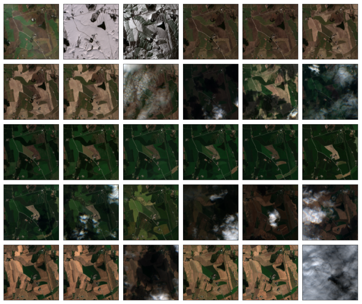
• Masking remote sensing images: To filter out pixels and extract relevant information from remote sensing images, masks were applied. The process of generating image masks involves three key steps, as explained in the state-of-the-art work in [7]. Firstly, the bounding box intersects with the cultivated fields for each farm, retaining only the coordinates corresponding to the cultivated areas within the satellite images. Next, the geographic map coordinates of longitude and latitude are converted to pixel locations within the satellite images. Since the images have dimensions of $100\times 100$ pixels, the bounding boxes delineate the borders of these images, with the top-left corner being (0,0) and the bottom-right corner being (100,100). Each point within the bounding box representing a cultivated field is then mapped to pixel coordinates based on its relative position within the bounding box. Finally, a matrix of zeros and ones is generated based on the locations of the cultivated fields, resulting in a $100\times 100$ binary matrix. This matrix serves as the mask, with ones indicating the presence of cultivated areas and zeros representing non-cultivated regions within the satellite images.
  This research effort generated additional masks for various types of remote sensing images. The mask creation process was based on the geometry of the farm obtained from disposed properties, which will be explained later in this manuscript, representing the arable land area of the farm. The coordinates of the farm’s location were utilised as the centre of the mask to ensure precise alignment with satellite images. Each pixel in the mask was assigned a Boolean value, where a value of true indicated that the pixel fell within a property boundary belonging to the farm. Prior to utilising remote sensing images, each channel of these images was multiplied by the corresponding mask. This operation effectively converted pixels outside the farm’s property boundaries to zero, thereby eliminating irrelevant information for subsequent modelling tasks. This process is visually depicted in Figure 4, where the left side illustrates four satellite images of the same farm, while the right side displays the same images with masks applied.
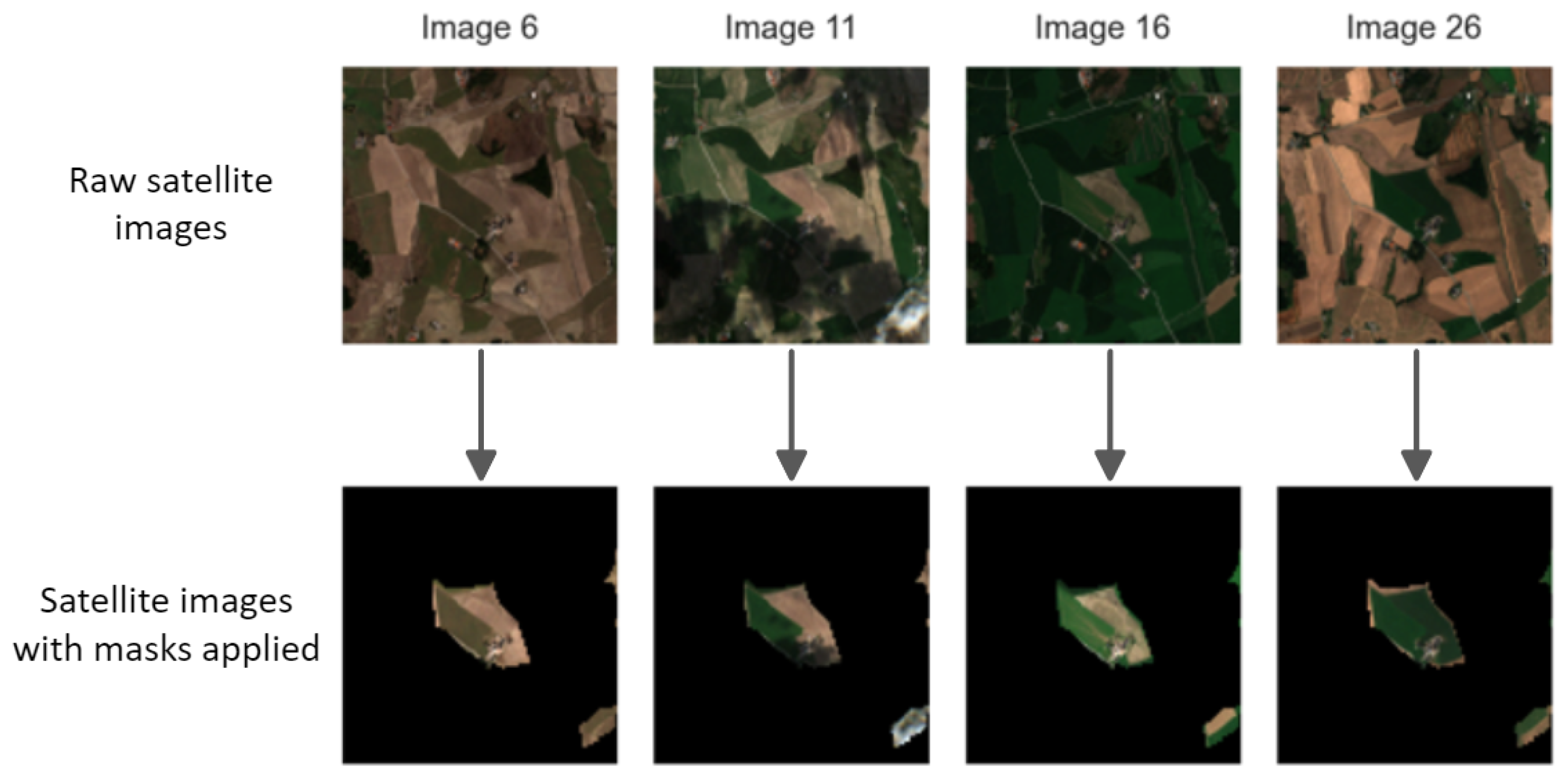
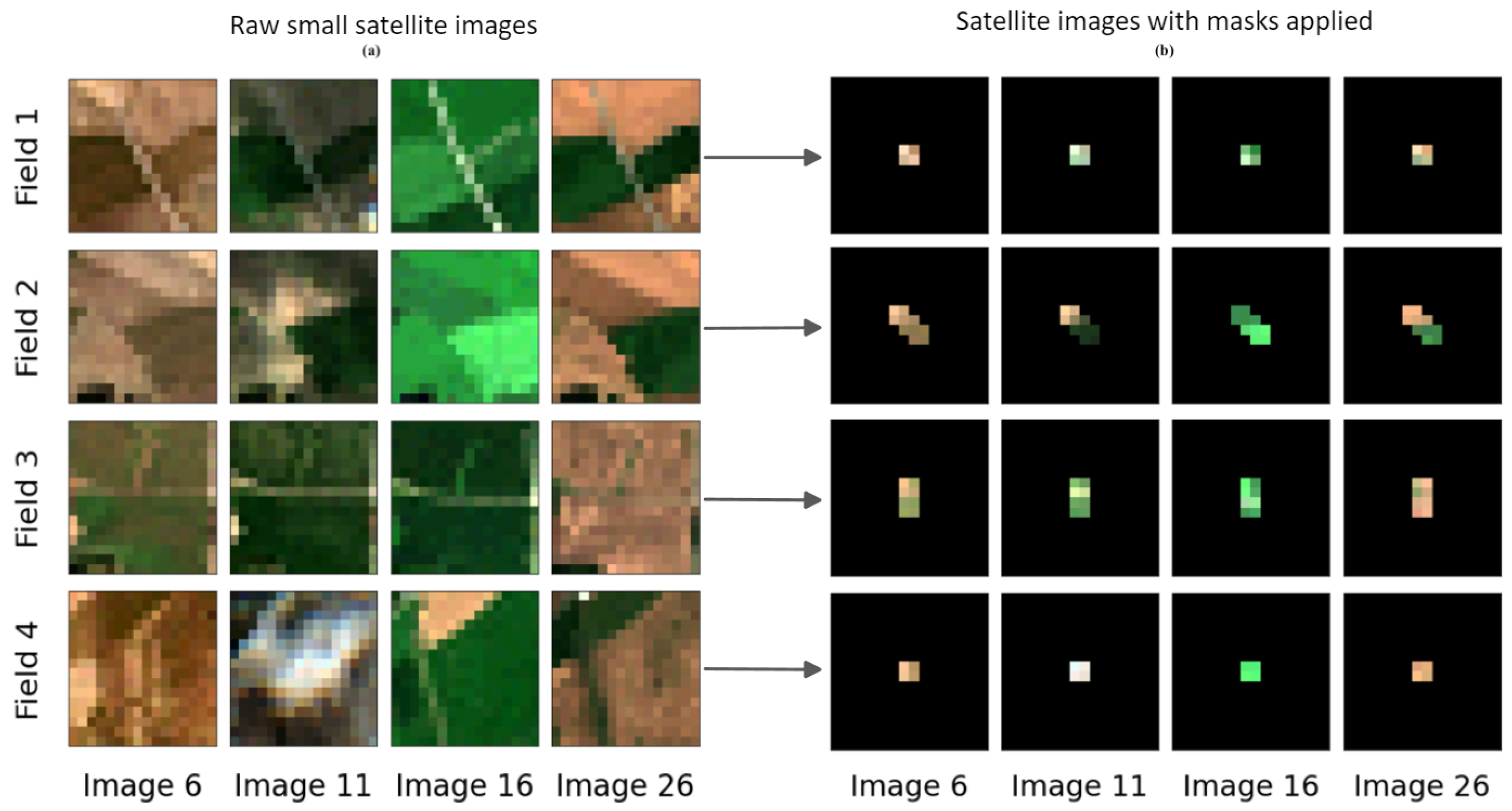
• Extracting field boundaries from remote sensing images: For the preliminary crop classification experiment, raw $100\times 100$ satellite images were employed. During experimentation, it became evident that each satellite image encapsulates information for multiple fields within a farmer’s farmland, often featuring different crop types. Consequently, applying a single crop type label to every image proved impractical. To address this, new field-based images with dimensions of $16\times 16$ were generated, each covering a single field. To facilitate the creation of these field-based images, the latitude and longitude for each farm and field were translated to values between 0 and 100, corresponding to its central position on the raw satellite image. In cases where the field’s position extended beyond the satellite image boundaries, an offset was applied. Once the field was correctly positioned, the satellite image was cropped using a $16\times 16$ side, as illustrated in Figure 5.
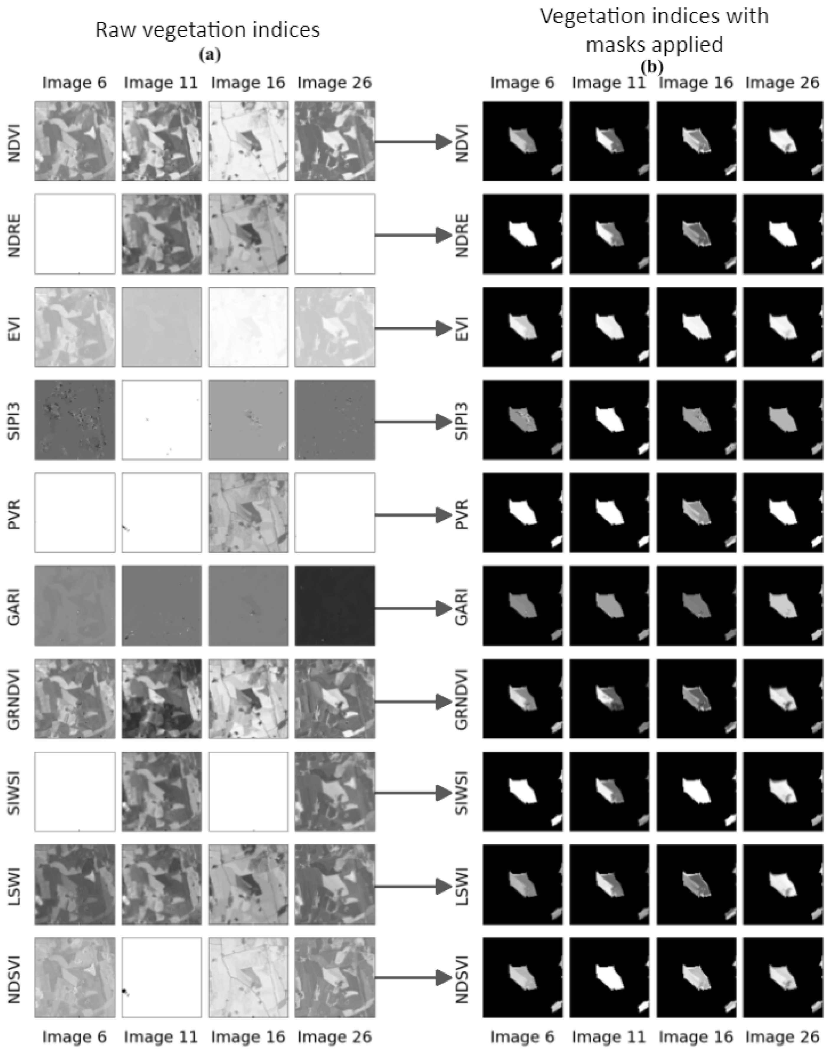
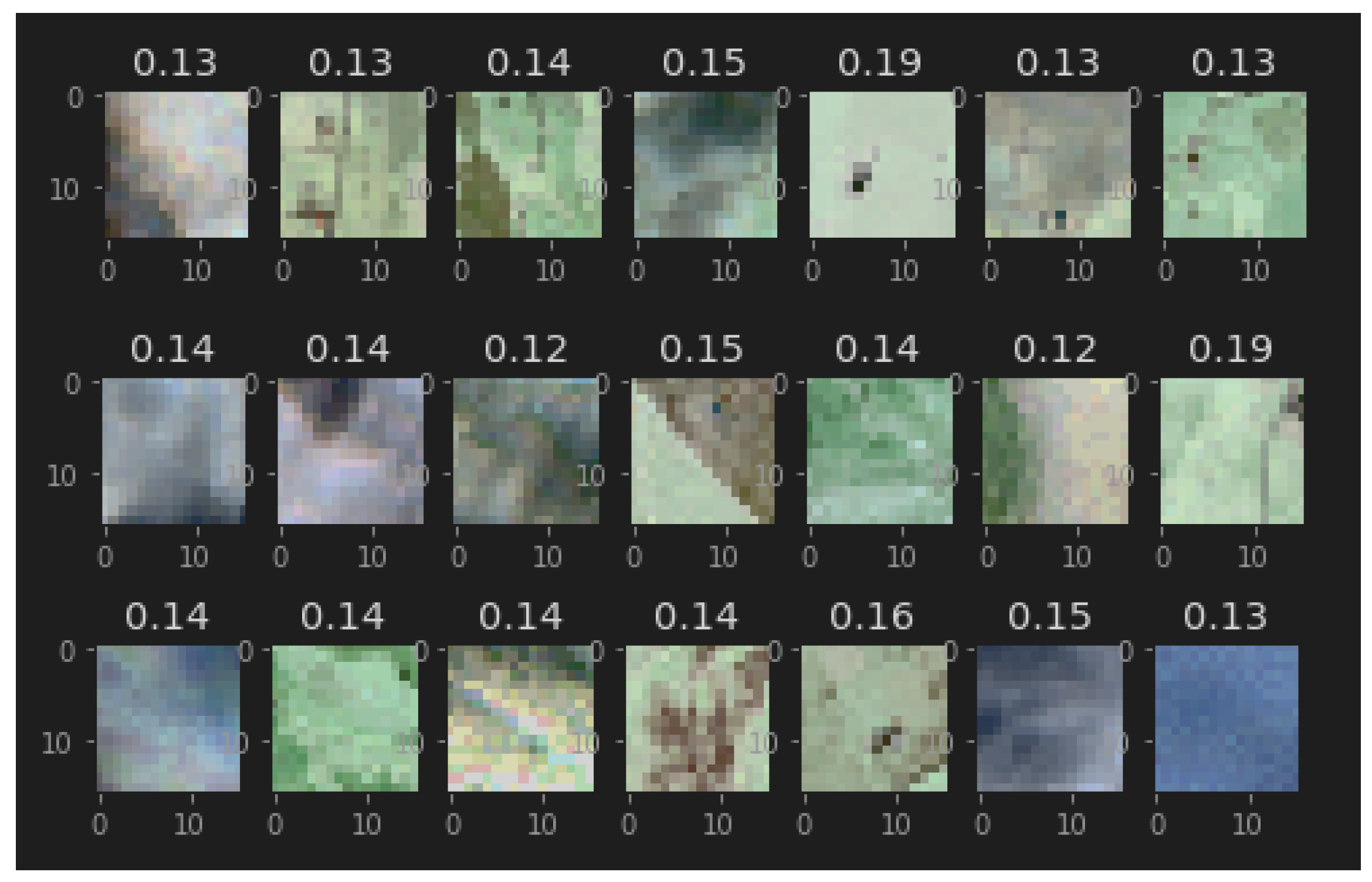
• Vegetation indices derived from satellite images: Throughout the literature reviewed in the previous Section 2.1.2, the efficacy of various vegetation indices for classifying and mapping crop types was demonstrated by several research efforts, including those by Hu et al. [15], Ma et al. [67], Wang et al. [47], and Barzin et al. [48]. These studies highlighted the utility of different vegetation indices derived from raw Sentinel images for agricultural applications. To identify suitable indices for Norwegian agriculture, a selection was made based on the findings of these research efforts.
  The appropriate Sentinel-2A bands for each vegetation index were determined using the wavelength information provided earlier in this manuscript, as well as studies by Kobayashi et al. [42] and Henrich et al. [26]. Subsequently, formulae were derived based on the theoretical foundations presented earlier. These formulae utilised the band numbers corresponding to the Sentinel-2A bands listed in Table 1. These calculations were performed to generate vegetation indices from every available raw satellite image, adhering to established methodologies and principles outlined in the literature.
  The vegetation indices were computed by extracting the relevant bands from the acquired Sentinel-2A satellite images and applying their respective formulae, as explained earlier in this manuscript. Ten vegetation indices were calculated for each of the 30 satellite images captured throughout the growing season for each farm. These indices were then stacked to form a $[30\times 100\times 100\times 10]$ image array. Examples of ten vegetation indices can be seen in Figure 6a, with the corresponding property masks applied that can be seen in Figure 6b. The images were normalised to a range between 0 and 1 to facilitate visualisation of the differences within the images. A greyscale representation was used as the images consist of a single channel. Blurry or blank areas in some images could be attributed to factors such as cloud cover, noise, limitations inherent to the vegetation index, or constraints in visualisation. A field-based dataset was constructed from the vegetation index images to facilitate classification using the vegetation indices, akin to the process employed for raw satellite images previously detailed in this section. Examples of two fields depicted using the NDVI, LSWI, and NDSVI vegetation indices are illustrated on the left side of Figure 7, with the corresponding field masks applied on the right side of Figure 7.

2.2.2. Geographical Data

The authors employed geographical data, which include disposed properties and coordinates, to delineate field shapes and boundaries. This excludes features such as trees, rivers, and mountains, which span the years 2017 to 2019. The disposed properties represent the intersection of the Norwegian cadastral data. The experimental findings revealed that, despite each farm being registered with a specific organisation number, they had distinct locations recorded at the Norwegian Brnnysund Register Centre (Brnnysundregistrene) (https://data.brreg.no/fullmakt/docs/index.html (accessed on 5 May 2024)). Inaccuracies in these registered locations could lead to misleading information, associating them with different properties within a city, sometimes distant from the actual farm. New longitude and latitude values were computed for the extracted polygons from the disposed properties data to address this issue. Updated coordinates effectively narrowed the geographical area, proving to be more accurate compared to the baseline study.

2.2.3. Temporal Meteorological Data

Temperature and precipitation were considered pertinent for plant growth in Norwegian agriculture, as indicated in [7,8]. Additional meteorological features (https://forages.oregonstate.edu/ssis/plants/plant-tolerances (accessed on 5 May 2024)), including the growth degree of the plant, sunlight duration, and the state of the land surface and soil (e.g., dry surface, moist ground, or frozen ground with measurable ice), were also extracted in this study.

2.2.4. Norwegian Grain Production Data:

The authors utilised official public archives containing farmer grant applications, production subsidies, and grain deliveries (https://data.norge.no/ (accessed on 5 May 2024)) from the Norwegian Agriculture Agency. Norwegian grain farmers, reliant on subsidies, annually submit grant applications detailing crop cultivation. The authors found three primary reports that served as foundational data: grain delivery reports specified quantities of barley, oats, wheat, rye, and rye wheat sold; agriculture production subsidies encompassed 174 features, including land area, crop types, and subsidies calculations; and a detailed report linked farmers’ organisation numbers to cadastral units. Consequently, the authors used grain production data from 2012 to the 2017 season, capturing historical yields and vital subsidy-related features for this research study.

3. Results

In this section, the authors evaluate and validate the baseline methodologies proposed in [7]. This assessment involves the augmentation of the agricultural data corpus to improve the overall predictive efficacy of grain yield. The authors precisely extract vegetation indices from satellite imagery to facilitate the classification of grains, concurrently evaluating the suitability of the attention-based multiple-instance learning (MAD-MIL) approach in the context of semi-labelled agricultural data. Furthermore, the authors apply these models to optimise early in-season yield predictions.

3.1. Baseline Approaches: Improving Grain Yield Predictions with DNN

In the preliminary phase of this experimentation, the authors extend the training dataset by incorporating supplementary features and additional data samples, surpassing the parameters defined in the baseline approach. Subsequent subsections explicate the individual testing of various methodologies.

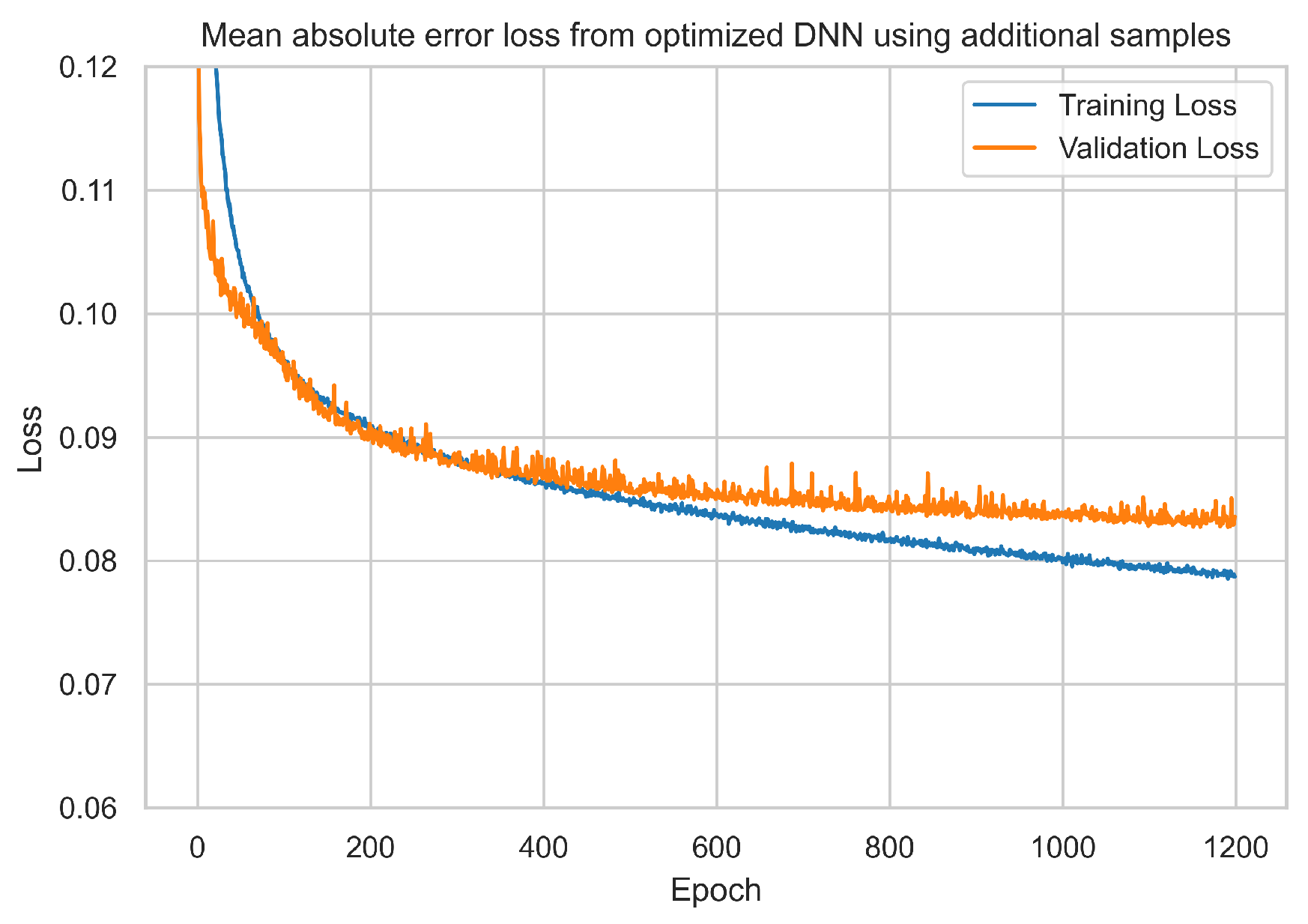
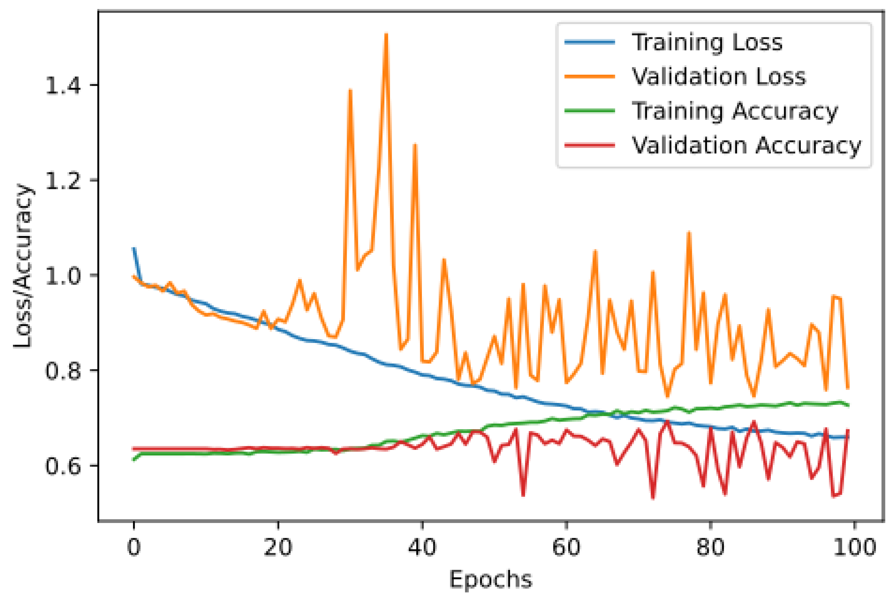
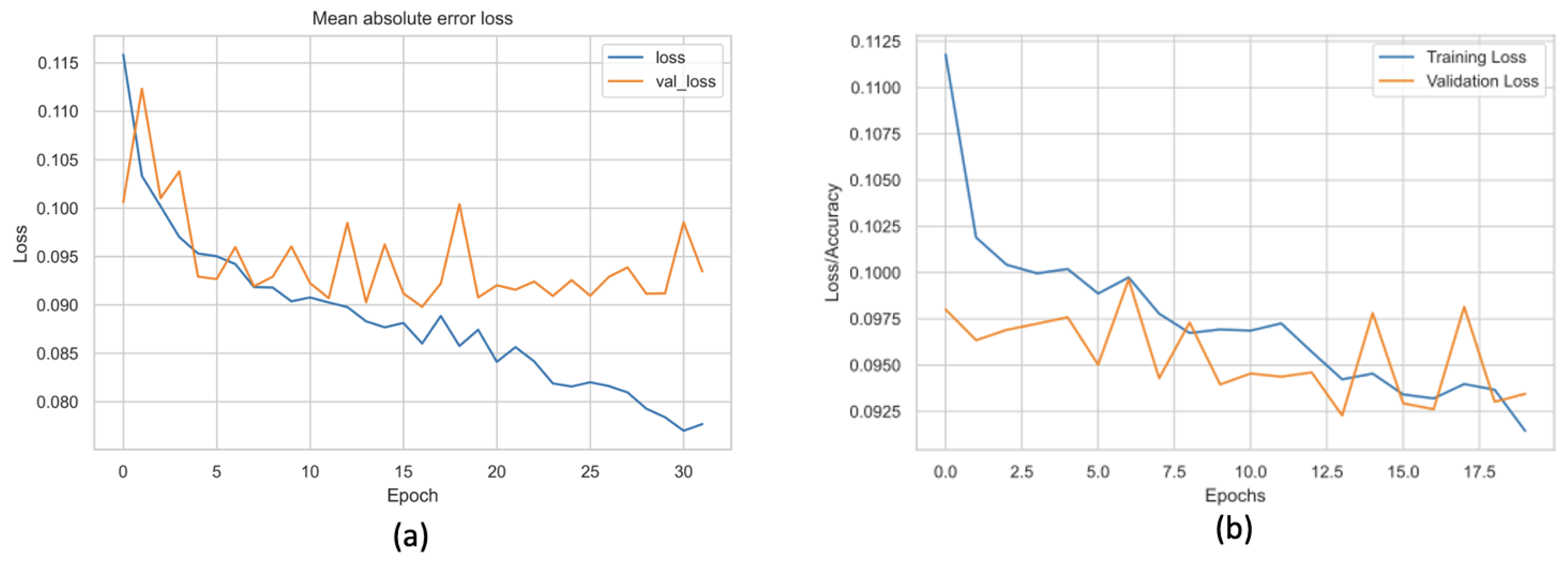
• Weather features to dense neural network: The authors enhance the utilised data by introducing three novel features—sunlight duration, state of the ground, and growth degree—into the training dataset. These additional features are integrated with farmer organisation numbers, expanding the feature count from 900 to approximately 1500. The authors subsequently re-implement the dense neural network (DNN), where the authors observed the initial signs of overfitting. Consequently, the model is adjusted by reducing the size of the first dense layer to 256 and marginally increasing the dropout percentages to 0.25 and 0.5, respectively. As illustrated in Figure 8b, a noticeably diminished disparity between training loss and validation loss is evident compared to Figure 8a, signifying mitigation of overfitting. The mean absolute errors (MAEs), measured in kg per 1000 m² for the baseline and the newly proposed optimised models, stand at 83.85 kg per 1000 m² and 83.28 kg per 1000 m², respectively; see

  Table 2. Summary of the baseline models to improve grain yield predictions.

  Baseline Approach	Validation Loss	MAE (kg/1000 m2)
  Baseline DNN	0.90	83.85
  New Features to Optimised DNN	0.82	83.28
  New Data Samples to Optimised DNN	0.84	82.82
  Integrated Features and Data to Optimised DNN	0.83	82.60

  and Figure 8. As a result, the authors opt to employ this newly proposed and optimised DNN model for subsequent experiments.
• Extended data corpus to dense neural network: The authors believe that augmenting the training dataset with additional data samples has the potential to improve accuracy. To substantiate this hypothesis, they re-implemented scripts sourced from the Frost API (https://frost.met.no/ (accessed on 5 May 2024)) to expand the weather data by 33% for 2020. Following this augmentation, the data underwent pre-processing, employing interpolation and normalisation techniques. The optimised dense neural network (DNN) model was subsequently trained for 1200 epochs, resulting in diminished loss values for both the training and validation sets. Furthermore, the mean absolute error (MAE) for this particular experiment was computed as 82.82 kg per 1000 m² (see Table 2 and Figure 9), closely resembling the performance of the optimised DNN model discussed earlier in this section.
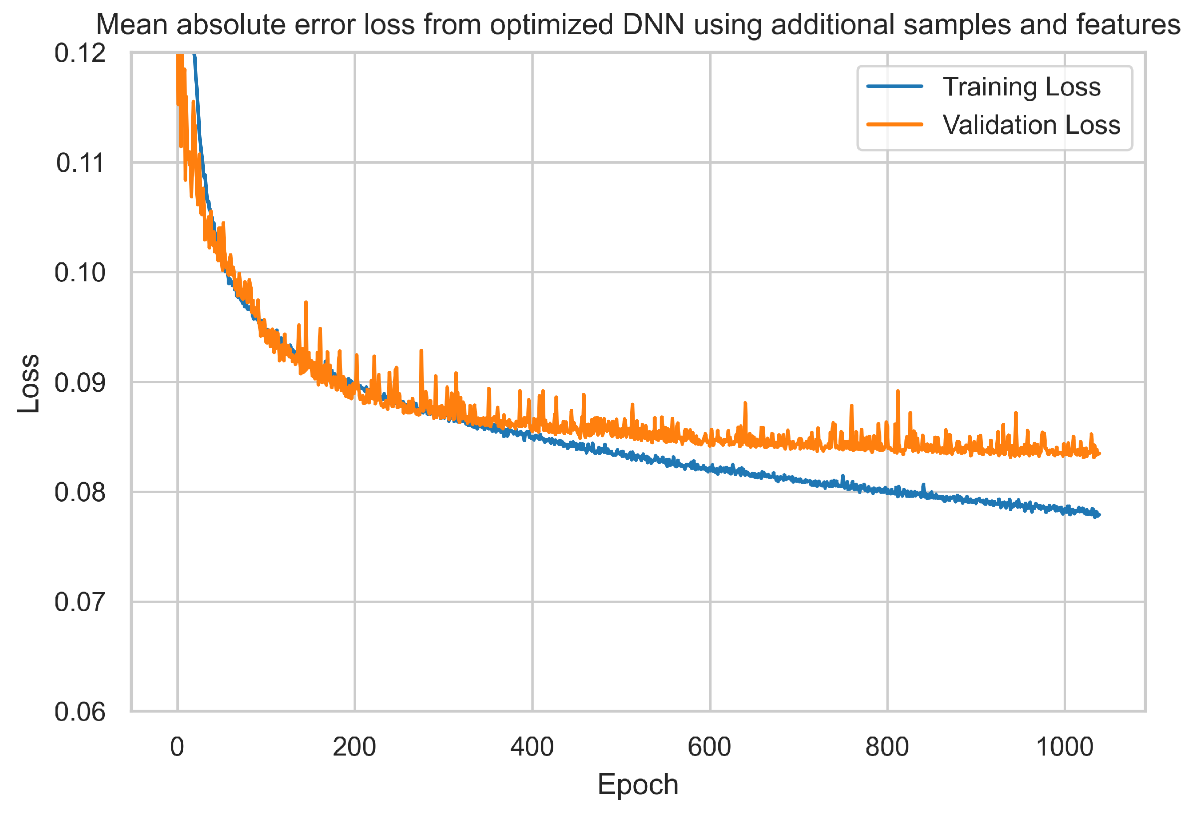
• Integration of features and data corpus to dense neural network: Following the integration of the dataset with additional weather features and data samples, as previously detailed, a further 600 features and approximately 15,000 samples were incorporated. The optimised dense neural network (DNN) model, adapted to accommodate the expanded input shape, underwent 1200 training epochs. As a consequence, the mean absolute error (MAE) value exhibited a marginal decrease of approximately 0.7 kg per 1000 m², which resulted in a value of 82.60 kg per 1000 m²; see Table 2 and Figure 10. Furthermore, a minor increase in training time of approximately 5 to 6 min was observed, attributed to the enlarged data corpus.

3.2. State-of-the-Art Approach: Improving Grain Yield Predictions with Hybrid CNN Model

The authors opted to re-implement the optimal approach outlined in [7] as the state-of-the-art methodology for refining grain yield prediction, acknowledging financial constraints that precluded the acquisition of additional satellite images for 2020. Instead, their focus shifted towards expanding the dataset with supplementary weather features (totalling 1500 features) and employing diverse augmentation techniques, such as salt and pepper, stride augmentations, and rotations, on satellite images from 2017 to 2019. Subsequently, the authors curated a time-series dataset encompassing yield values, weather features, and features derived from grain production data for each image. They re-implemented the hybrid convolutional neural network (CNN) model for the training phase. Each feature was inputted, concatenated, and fed into the gated recurrent unit (GRU) layer. The data were then flattened and processed through two dense layers. Adam served as the optimiser, with a learning rate of 0.001, and an early stopping callback with a patience value of 10 was incorporated. The resultant mean absolute error (MAE) value was 78.9 kg per 1000 m²; see

Table 3. Summary of the best-performing baseline and state-of-the-art models to improve grain yield predictions.

Best-Performing Approaches	Validation Loss	MAE (kg/1000 m2)
Integrated Features and Data to Optimised DNN	0.83	82.60
New Features to Hybrid CNN	0.79	78.96

. This signified a 2.53 kg per 1000 m² increase compared to the optimal results achieved with the hybrid model.

In conclusion, the justification for extending the agricultural data corpus to enhance grain yield predictions is evident, as presented in Table 3. Improved values for validation loss and mean absolute error (MAE) were achieved by incorporating fused features and additional data samples into the dense neural network (DNN) model, as well as by introducing new features into the top-performing hybrid convolutional neural network (CNN) model from [7]. It is important to note that these predictions are contingent upon the growing season in Norway, thereby limiting the applicability of the prediction models to the pre-growing season period. While the preceding research study has attempted to predict yields early on without knowing the specific crop planted in each field, the authors believe that exploring the classification of each crop type within a particular field area could provide a more practical real-life application for farmers in facilitating early in-season yield predictions. Consequently, the authors explore novel approaches for grain classification and early in-season yield predictions in the forthcoming sections.

3.3. Novel Approaches: Improving Early In-Season Grain Yield Predictions with Grain Classification Models

For the upcoming experiments about grain classification, the authors employed multi-spectral satellite images representing a specific geographic location in conjunction with the previously explicated vegetation indices. Initially, the authors introduce an artificial intelligence (AI) model designed for grain classification at the farm scale. Despite the observation that each farm image encompasses multiple fields with distinct grain types, the proposed model is trained with a focus on field-based grain classification. Vegetation indices are employed to enhance the overall assessment of this model and ascertain the optimal timing for classifying a diverse array of grain types. Additionally, they present the semi-labelled agricultural data discussed earlier in this paper, which undergoes training through an attention-based multiple-instance learning model (MAD-MIL). This approach enhances the performance of grain classification, specifically within the agricultural context of Norway.

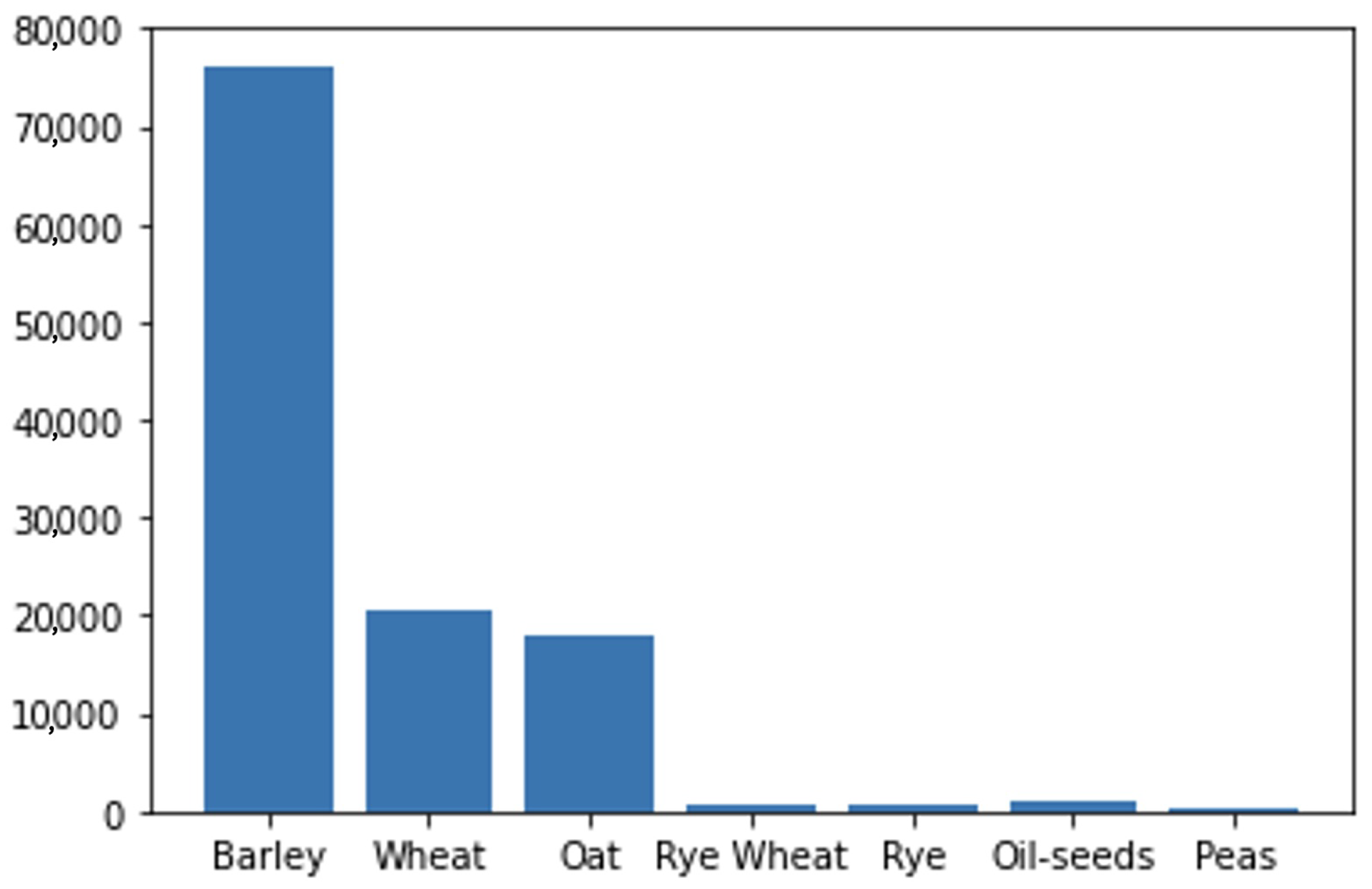
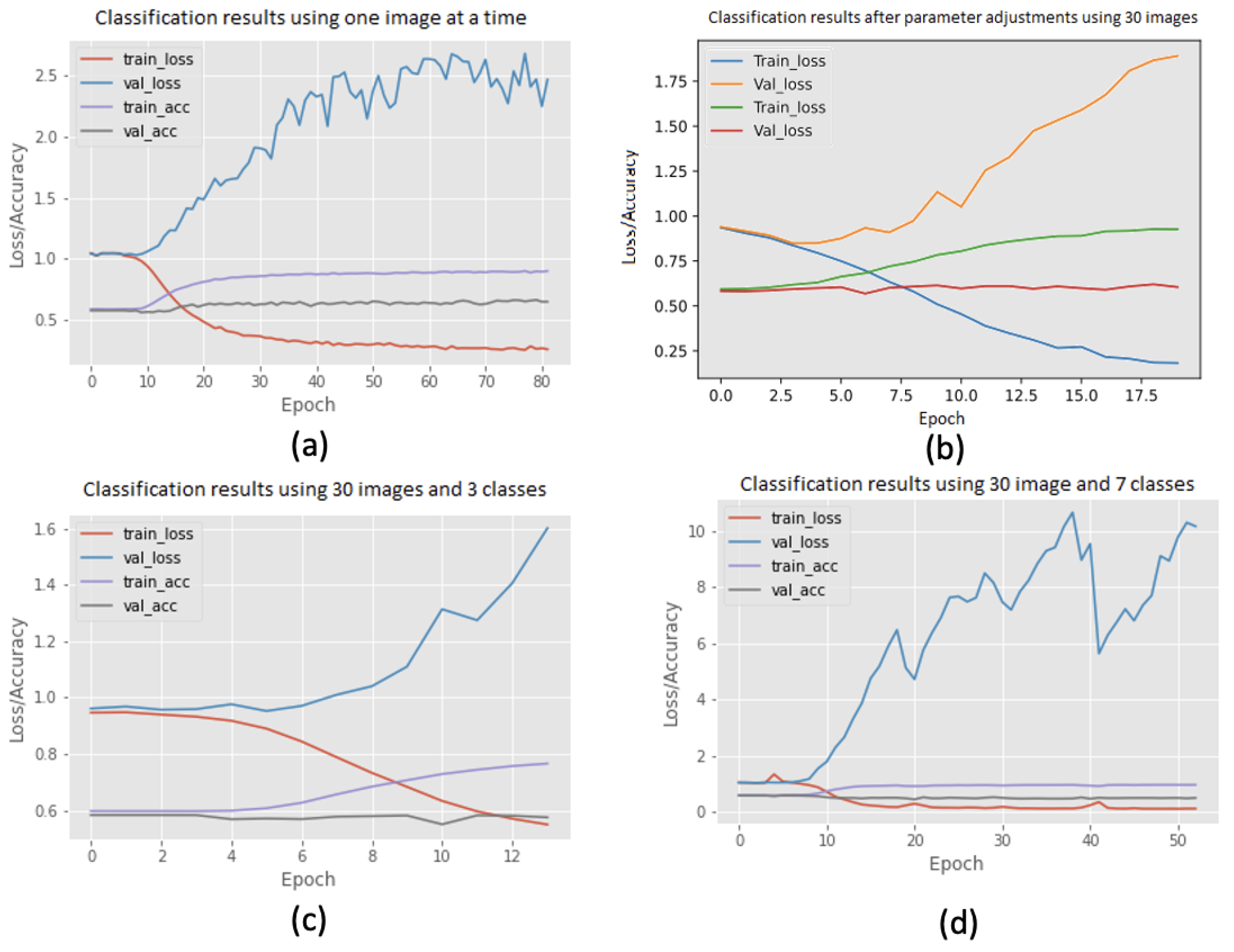
• Farm-scale grain classification: The proposed model for farm-scale crop classification is designed to ascertain the crop type planted on a given farm based on a time series of 30 satellite images. The classification dataset operates under the assumption that all fields associated with a particular farm contain a singular crop type. This assumption raises concerns regarding the reliability of results, as the classification dataset lacks a foundation in ground truth, as previously discussed. Furthermore, the images may incorporate significant noise, such as clouds, potentially leading to misguidance of the classification model. Consequently, the authors implemented image masking and data augmentation techniques during training. The initial classification model utilised the convolutional neural network (CNN) and gated recurrent unit (GRU) components of the hybrid model. In this architecture, the GRU encodes the entire time-series data sequence into a 64-length vector, then flattens it. The final dense layer of the model, employing a softmax activation function, generates a vector with percentage predictions for each crop type. However, this model exhibited a tendency to overfit due to the limited number of images used in the time-series data.
  As illustrated in Figure 11, barley, wheat, and oats are extensively cultivated in Norway, while the four less prevalent crop classes—rye wheat, rye, oil seed, and peas—exhibit lower prevalence. The authors posit that rectifying this imbalance by excluding the less prevalent crop classes could contribute to a more balanced dataset, thereby enhancing model performance. Consequently, the authors explored four distinct variations in experimentation: inputting one image at a time from the 30-image time series (see Figure 12a), inputting all 30 images with hyper-parameter adjustments (see Figure 12b), inputting all 30 images with three crop classes (see Figure 12c), and inputting all 30 images with all seven crop classes (see Figure 12d). Various attempts were made to adjust network hyperparameters, eliminate crop type classes with low occurrences, and implement exponential learning rate decay with diverse parameters to alleviate overfitting. Unfortunately, these adjustments did not yield improvements, prompting consideration for field-based crop classification. It is evident from the results that the training loss exhibits a declining trend throughout the experiments, indicating that the model assimilates certain features and subsequently enhances training accuracy.
  Moreover, the validation accuracy predominantly remains constant, even after training for 80 epochs, and in most cases, the validation loss experiences an increase. The distinct models underwent varying amounts of processing time as each experiment manifested a consistent negative trend; see Figure 12. The graphical representations illustrate that the validation accuracy consistently hovers around 0.6 for all implemented models. The initial random image model achieved its highest training accuracy at 0.8; however, acknowledging its tendency for overfitting, the authors decided to explore the field-based grain classification to enhance target analysis.
• Field-based grain classification: The field-based crop classification model categorises crop types based on time-series images of individual fields rather than the entire farm. This approach offers the advantage of reduced noise in the images, leading to a faster training process. The creation of field-based images is detailed earlier in this manuscript. These images have dimensions of $16\times 16\times 12$, sufficiently large to encompass even the most extensive fields while remaining significantly smaller than the original size. The fields with the smallest areas were excluded from consideration, as these would cover only one or two pixels in the satellite images, providing minimal data for the network. This exclusionary criterion was applied to all subsequent experiments related to field-based crop classification. Moreover, the satellite images underwent augmentation techniques such as salt and pepper, rotation, and random flips. Augmentation was incorporated due to its efficacy in mitigating overfitting in machine learning models. Subsequently, the images were integrated into a TensorFlow Generator and inputted into the model. During the reconstruction of the model for field-based images in this experiment, inspiration was drawn from a study by Ferlet (https://medium.com/smileinnovation/training-neural-network-with-image-sequence-an-example-with-video-as-input-c3407f7a0b0f (accessed on 6 May 2024)) to further enhance model performance. Additionally, the successful 2D CNN implementation with multiple sets of CNN, max-pooling, and ReLU by Kussul et al. [12] was evaluated. The researchers achieved a crop type classification accuracy of 94.6%. Therefore, their architectural structure and functions were considered and evaluated for application in this experiment.

This model, characterised by several layers and neurons, prompted the selective incorporation of pertinent network layers tailored to the agricultural data to mitigate overfitting. Resembling the farm-based model, this model diverges in the time-distributed part, featuring additional parameters like moving mean and variance, beta, and gamma inherited from the batch normalisation layers in the CNN net. Additionally, an extra dense layer, encompassing a dropout layer, is introduced post-GRU, with these dense layers being smaller than their farm-based counterparts. Notably, the GRU layer’s size is reduced to 12 units from 64 units, impacting its effectiveness in preventing overfitting. Figure 13 illustrates the outcomes of training the optimised field-based crop classification model, revealing a decline in loss and increase in accuracy for both training and validation sets—a discernible improvement compared to the farm-scale model. At its best, this model achieved a validation accuracy of 70%, representing a 10% enhancement over farm-scale classification. These findings substantiate that smaller, less noisy images are more conducive to accurate crop classification. Moreover, fluctuations in validation loss and accuracy after 20 to 30 epochs are observed, a topic to be addressed in subsequent sections. Additionally, a possibility for overfitting is noted in most crop classification results, a phenomenon recurrently identified due to data distribution, particularly in datasets featuring satellite images.

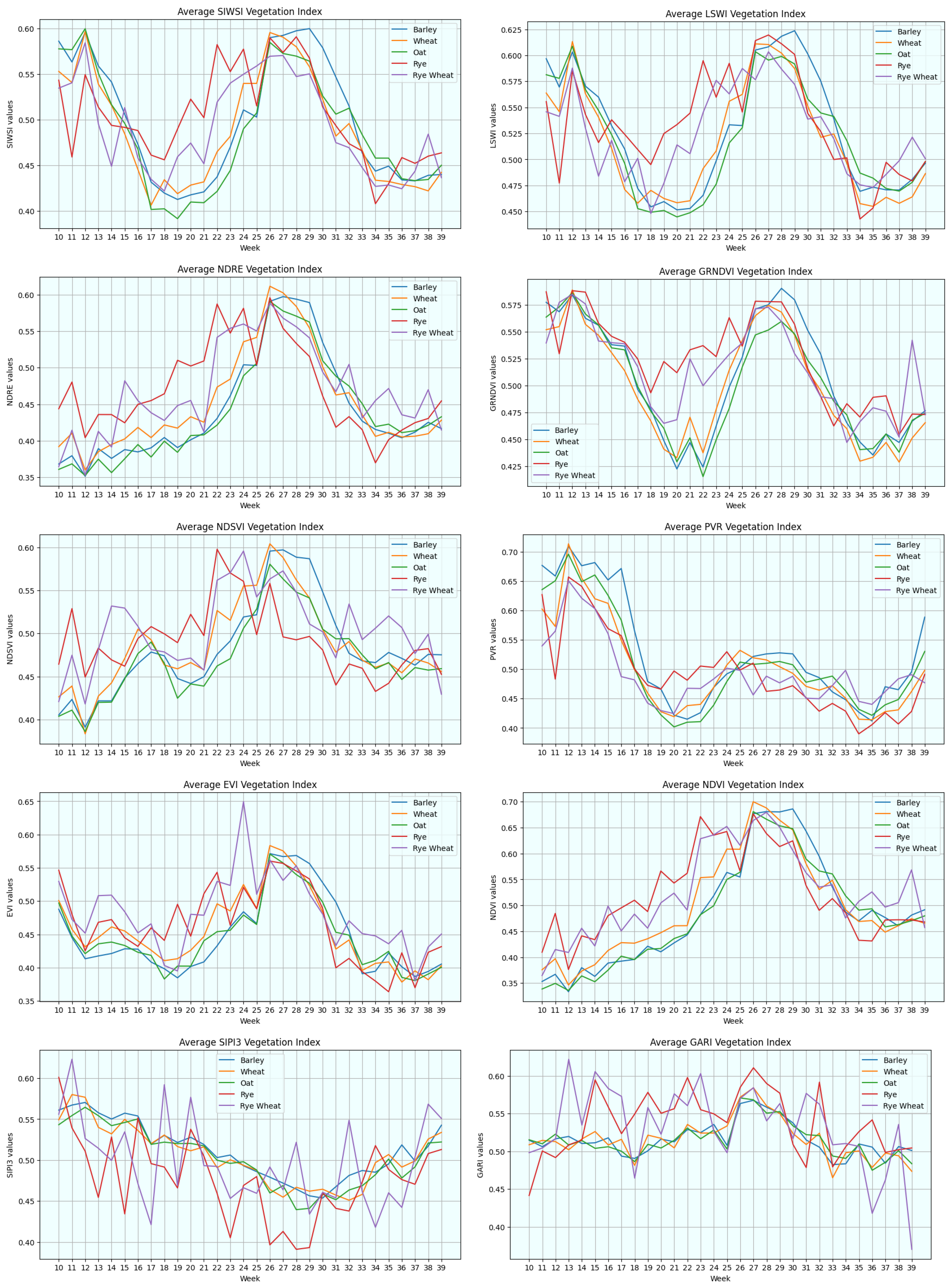
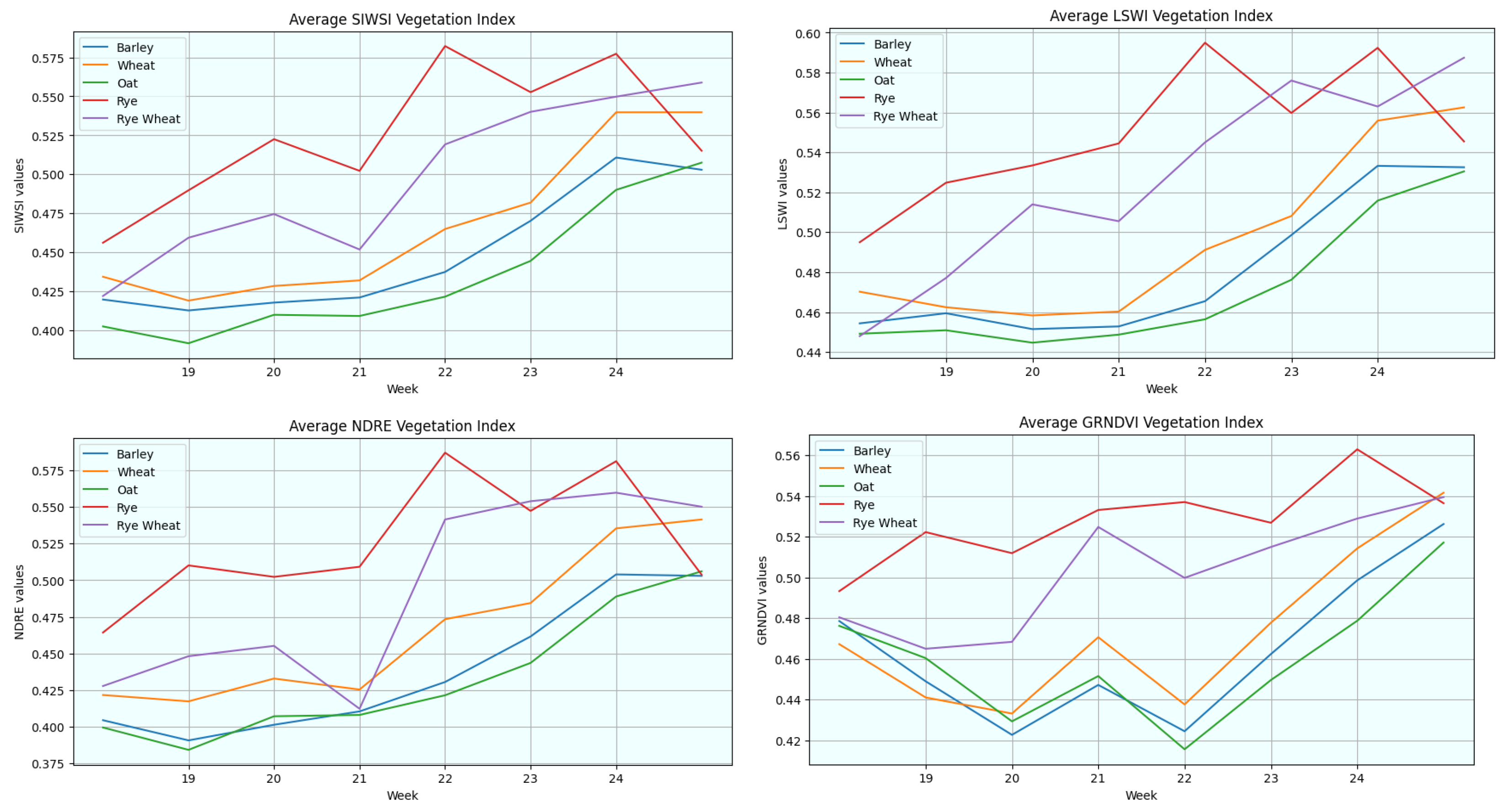
• Improving field-based grain classification using vegetation indices: As delineated in Section 2.1.2, the average temporal profiles of vegetation indices were computed for each crop type throughout the growing season. Given the many crop types across ten distinct graphs, the visual representation could become convoluted and challenging to interpret. Consequently, the results for oil seeds and peas were excluded for streamlining the presentation and focusing on the most pertinent information, as they hold lesser relevance to crop classification and crop yield analysis. Figure 14 displays graphs of the five primary crop types. Each graph in Figure 14 illustrates the temporal trajectory of a specific vegetation index, with individual lines representing different crop types. While some graphs may appear similar superficially, a closer examination reveals meaningful insights about the vegetation indices. Many indices exhibit a common trend in their temporal development, characterised by gradual growth throughout the growing season until reaching a peak, likely indicative of crop maturity, followed by a sharp decline during harvest.

While the overall development and shape of the vegetation indices are pertinent for studying grain yields, the crucial aspect of crop classification lies in discerning the differences between crop types at any given week. Notably, a distinct trend emerges between weeks 18 and 25, wherein the indices begin to distinguish between each crop type more prominently. Through a systematic feature elimination process, specific time periods and vegetation indices were systematically discarded until an optimal combination was identified, wherein each index exhibited clear differentiation between crop types consistently throughout the entire period. Figure 15 showcases the optimal combination of vegetation indices, including the SIWSI, LSWI, NDRE, and GRNDVI, within the time frame spanning weeks 19 to 24. Notably, not only are the differences between each crop type pronounced and consistent, but the graphs also demonstrate minimal overlap, underscoring the efficacy of this selection.

For the field-based grain classification experiments, images of size $30\times 16\times 16\times 12$ were generated, as discussed earlier, along with corresponding field masks. These images were subsequently applied to the aforementioned farm-scale grain classification model for two distinct experiments. The first experiment targeted five relevant crop types, while the second focused on all seven for yield prediction. Both experiments exclusively utilised vegetation indices derived from satellite images captured between agriculture-specific weeks 15 and 30. The exclusion of early-week images was motivated by the prevalence of snow, cloud cover, atmospheric disturbance, and other forms of noise in these early satellite images. Similarly, the omission of the latest images aligned with the experiment’s objective of identifying crop types early in the growing season. Simultaneously, the previously optimised classification model, detailed earlier in this section, was re-implemented. Weekly application of all indices derived from the five crop types to the optimised model ensured the incorporation of a comprehensive set of features, maximising the utilisation of the entire data distribution. In light of persistent challenges, insights from Pea-Barragán et al. [58] were considered, indicating that images from late summer and mid-spring contribute 60% and 30% to classification learning, respectively. Consequently, a fourth experiment was conducted, utilising images from weeks 30 to 39 to account for the 60% contribution from the latest weeks. Furthermore, to enhance the overall model performance, the work of Foerster et al. [14] on plotting and studying vegetation indices throughout the growing season was considered. The researchers devised temporal profiles for each vegetation index, calculating average values for the ten indices utilised in every image through a systematic process outlined as follows:

• The farm’s field masks, as outlined in the previous section, were applied to their respective locations to exclusively utilise vegetation index values from fields.
• For each vegetation index image, the values were normalised within the range of 0 to 1. Subsequently, the average of these normalised values was calculated and stored. This process was executed for every vegetation index image for each farm’s 30 images annually.
• The averages computed in the preceding step were aggregated across all images to derive an average of the averages. Notably, this aggregation was performed while filtering for crop type, signifying that each vegetation index yielded an average weekly value specific to each crop type.

These procedures yielded average vegetation index values for each crop type in every satellite image. The analytical approach facilitated the evaluation of the potential of each vegetation index for crop classification. Building on this understanding, the indices were further explored to identify the optimal period and the most distinguishable vegetation indices. In each experiment involving crop classification with vegetation indices, a diverse set of learning rates, layer sizes, and crop and time intervals were tested, with and without masks, demonstrating no noticeable changes. Consequently, the validation loss and accuracy from each significant experiment are summarised in

Table 4. Crop classification experiments using vegetation indices [17].

No.	Vegetation Indices	Model	Crop Types	Week Interval	Val Loss	Val Accuracy
1.	All	Initial	Five Types	15–30	0.8910	0.6423
2.	All	Initial	All Types	15–30	0.9745	0.6330
3.	All	Optimized	Five Types	10–39	0.9222	0.6366
4.	All	Optimized	Five Types	30–39	0.9247	0.6353
5.	Optimal	Initial	Five Types	19–24	0.9498	0.6359
6.	Optimal	Optimized	Five Types	19–24	0.9520	0.6353

below.

The initial two experiments focusing on grain yield classification exhibited marginal improvements regarding the least validation loss and the highest validation accuracy compared to other experiments, as outlined in Table 4. The outcomes of the third experiment involved the application of all vegetation indices throughout the growing season. The fourth experiment exclusively utilised the last ten-week intervals from the growing season. The results presented in Table 4 for the fifth and sixth experiments emanate from the model trained using the optimal vegetation indices and time periods discussed earlier in this section. Notably, the application of optimal vegetation indices resulted in what can be considered negligible changes in both validation loss and accuracy. Surprisingly, endeavours to enhance the classification model and optimise the applied data distribution for vegetation indices yielded no observable improvements. This outcome is likely attributable to factors such as noisy satellite images and inherent limitations in the vegetation indices. A comprehensive discussion of these factors will be undertaken in future work, detailed in the subsequent section.

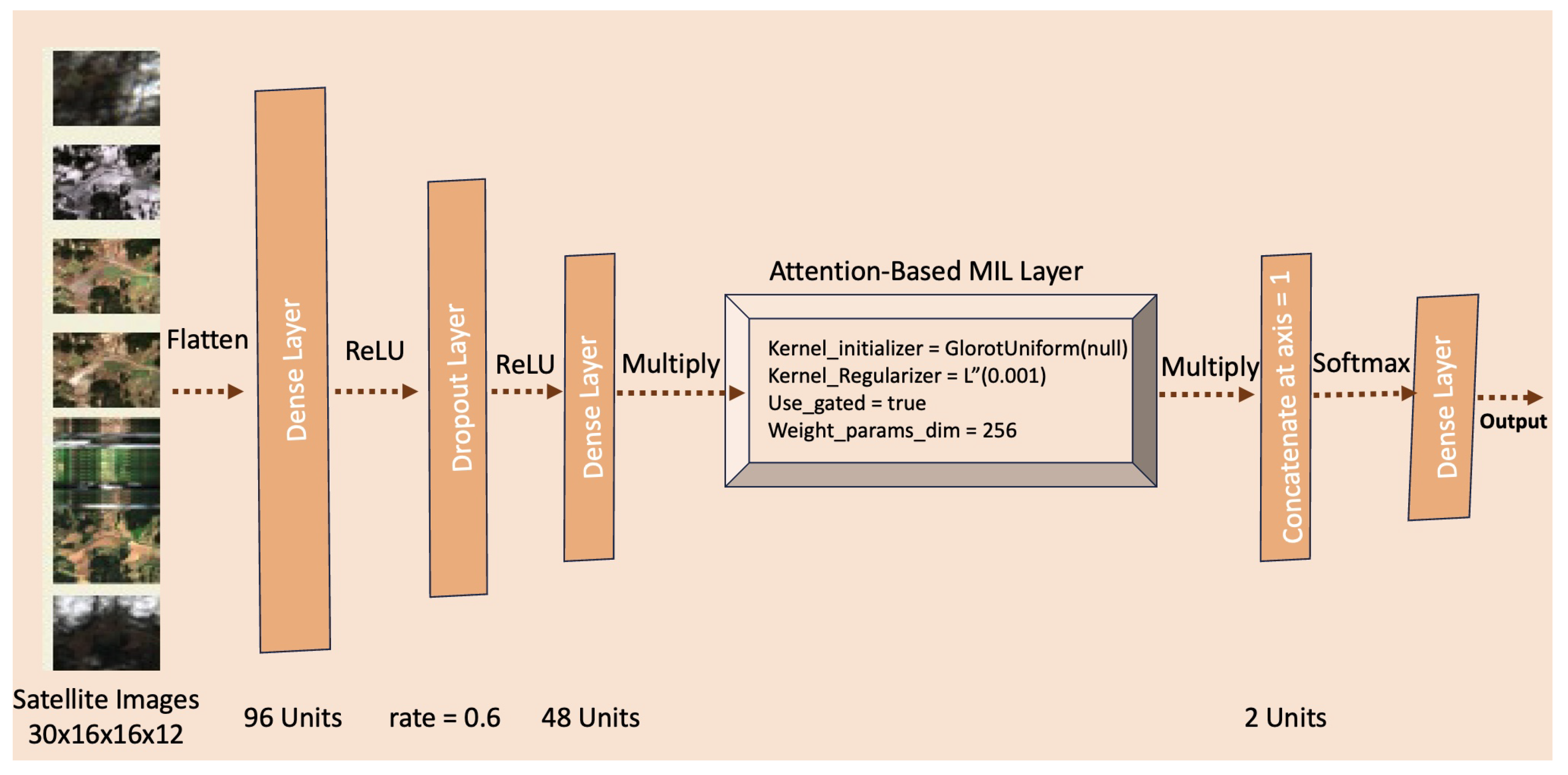
• Multi-class attention-based deep multiple-instance learning (MAD-MIL) to grain classification: As discussed earlier in this paper, the labelling of raw satellite images for a single crop type was unfeasible due to the fusion of information from multiple fields within each image. Consequently, the acquisition of semi-labelled agricultural data became imperative. To train this semi-labelled data effectively, the authors proposed implementing a multi-class attention-based deep multiple-instance learning (MAD-MIL) model, anticipating better results. The MAD-MIL model (https://keras.io/examples/vision/attention_mil_classification/ (accessed on 6 May 2024)) was realised with TensorFlow and Keras’ implementation serving as the foundation. Subsequently, the dataset was partitioned into training and validation bags, employing distinct parameters and an optimal bag size. Through experimentation, selecting a bag size of seven aimed to strike an optimal balance between positive and negative bags. The neural network was trained utilising the Adam optimiser with a learning rate 0.001, spanning 150 epochs. Various bag sizes were explored, including 100, 200, 300, 500, and 750. Additionally, validation bag sizes were adjusted within the range of 100 to 250, contingent upon the chosen training bag size. These meticulous considerations were made to ensure the effectiveness of the MAD-MIL model in capturing relevant features and patterns within the semi-labelled agricultural data.

Figure 16 illustrates the architectural layout of the implemented MAD-MIL model. Each input layer is dedicated to an individual bag, encompassing a series of 30 field images. These images are flattened before traversing through two dense layers, interspersed with a dropout layer featuring a rate of 0.6. The subsequent attention layer calculates attention scores, followed by concatenation. Ultimately, the data are channelled into the final dense layers, consisting of two units each and employing a softmax activation function. The utilisation of two units is necessitated by the binary classification nature of each bag, categorised as either negative or positive. The MAD-MIL model’s efficacy is gauged through accuracy, quantifying the correct classification of bags as positive or negative. A distinct model was created for each crop type, as the MAD-MIL model necessitated the designation of a single class as the positive one during bag creation. Additionally, the model computed attention scores for each sample within every bag during training. In the event of a positive classification, the samples—fields resulting in a positively predicted bag—were assigned the label associated with the highest attention score. Consequently, leveraging these attention scores, each model could classify all of the encompassed crop types. The ensuing section presents the outcomes of the MAD-MIL experiments, featuring varying numbers of bags.

Table 5. Validation accuracy achieved from MAD-MIL models with a different number of bags.

Crop Type	Metric	100 Bags	200 Bags	300 Bags	500 Bags	750 Bags
Barley	Accuracy	0.73	0.62	0.66	0.64	0.74
Barley	Loss	0.67	0.64	0.62	0.61	0.60
Wheat	Accuracy	0.71	0.70	0.73	0.67	0.68
Wheat	Loss	0.65	0.95	0.64	0.62	0.67
Oat	Accuracy	0.56	0.59	0.60	0.63	0.60
Oat	Loss	0.71	0.69	0.68	0.68	0.67
Rye	Accuracy	0.96	0.97	0.98	0.99	0.99
Rye	Loss	0.37	0.47	0.45	0.48	0.48
Rye Wheat	Accuracy	0.96	0.97	0.98	0.99	0.97
Rye Wheat	Loss	0.21	0.15	0.60	0.09	0.21

presents each model’s accuracy and loss outcomes across diverse parameters, with the optimal results highlighted. Noticeably, barley, wheat, and oats exhibit comparable performance, while rye and rye wheat show significantly higher accuracy and lower loss values. Furthermore, superior results are attained when employing a more significant number of bags as training data, with accuracy showing an upward trend and loss demonstrating a downward trajectory as the number of bags increases. The rationale behind these observed patterns will be expounded in the subsequent section.

Figure 17 illustrates the attention scores extracted from one of the trained MAD-MIL models. The figure shows three bags, with each row representing a bag and utilising a bag size of seven. The initial two rows correspond to positively predicted bags, while the last refers to a negatively predicted bag. Notably, this specific model was trained with barley designated as the positive label. Moreover, noticeable variations in attention scores are observed among instances (field images), with some instances attaining higher scores than others. For example, the two fields that received a score of 0.19 likely indicate a field containing barley. In contrast, the scores in the bottom row exhibit a more equal distribution.

3.4. Novel Approaches to Early In-Season Grain Yield Predictions

Two distinct models were developed for early yield prediction and crop classification, focusing on targeted in-season predictions. The datasets utilised for these models encompassed information collected exclusively during the growing season, with the exclusion of data obtained from grain delivery or farmer’s subsidies. While this dataset contained fewer instances than the one utilised in the baseline approach [7,8], it was deemed more suitable for in-season predictions. This strategic choice aimed to enhance the models’ practicality, aligning them more closely with real-life scenarios and rendering the predictions more applicable for real-time agricultural decision-making.

3.4.1. Implementing Early Crop Type Classification

For this experiment, the authors aim to utilise satellite images from weeks 10 to 26 and 10 to 21 to predict classes on labelled and unlabelled data. Subsequently, the outcomes of this model are employed as input for the reconfigured yield prediction models. The primary motivation for conducting this experiment is to create a model that relies on data acquired early in the growing season, rendering it more applicable to real-life agricultural scenarios. Unlike models necessitating data from week 30 onward, such an approach eliminates the impracticality of waiting for crop type information long after the growing season concludes. The data pre-processing, model implementation, and training closely mirror the field-based crop classification process outlined earlier in this section. The primary distinction lies in the quantity of images fed into the network, resulting in a corresponding adjustment in the network’s input shape. The decision to refrain from using the MAD-MIL model for crop type prediction stems from its inability to generate precise and easily applicable results for the early yield models. Consequently, the field-based classification model is the foundational template for the early in-season crop type prediction model. Various amounts of satellite imagery are incorporated into the network by adjusting the iterator supplied to the TensorFlow Generator. Both classification models adhere to identical parameters used in the field-based grain classification model during training. Once trained, the model generated from this experiment is deployed to predict crop types across all field data, excluding fields with a small area. Subsequently, a file containing information on the crop type associated with each field is generated. This file serves a dual purpose: It facilitates the creation of masks for each farm and crop type, ensuring the yield prediction model exclusively employs the correct fields for predicting yields. Additionally, it functions as a lookup table for the crop type input feature, a key component in this innovative approach to early yield prediction.

As illustrated in Figure 18, the implementation includes loss and accuracy values for the proposed classification models using data from weeks 10–26 and weeks 10–21. The model’s ability to learn from the training data, attaining an accuracy of 70% for both models, is evident in Figure 18a,b. However, after critically observing the validation losses, it is revealed that the models face challenges when exposed to the validation data. Despite these validation losses, the models manage to achieve an approximate 63% validation accuracy, providing valuable insights and justifying the progression to the subsequent experiment for early in-season grain prediction.

3.4.2. Implementing Early Grain Yield Prediction

By performing this experiment, the authors aim to recreate the state-of-the-art work where the researchers attempt early predictions. Utilising their experiment as a framework, the authors integrated the novel features as detailed earlier in this paper. Additionally, the authors introduced the predicted crop type as a feature, identified by the organisation number, year, and field. Two models were constructed, similar to the early crop type prediction models. This approach investigated whether in-season early predictions remain successful when relying on predicted crop types. The necessity to predict crop types arises from the unavailability of crop type data during the growing season, requiring extraction from grain delivery data. The comprehensive dataset, encompassing satellite and numerical data, covers an entire growing season and all 30 weeks. The authors considered that some numerical data comprise multiple features daily to restrict the dataset to weeks 10–21 and weeks 10–26. Thus, data from day one to day 84 (12 × 7) of the growing season were retained by filtering the numerical data frame using a regular expression on column names. Each feature with daily data was then filtered and merged with the satellite images, ensuring inclusion only from columns named with the feature and a day number ranging from 0 to 84, corresponding to weeks 10–21.

Table 6. The mean absolute error (MAE) achieved using different time periods with the hybrid early yield prediction CNN. The MAE is compared to the previously achieved state-of-the-art values, using the same settings.

Input	Description	Previous MAE	Achieved MAE (kg/1000 m2)	Change
Weeks 10–39	Full season	76.27	78.96	3.53%
Weeks 10–26	Late June	82.11	89.77	−9.33%
Weeks 10–21	Mid-May	92.20	93.45	−1.35%

presents the results obtained from the two selected time intervals early in the growing season. Notably, the results demonstrate comparability and a lack of significant deterioration compared to the previous outcomes. The authors observe that these results were achieved with a reduced dataset and, more crucially, exclusively using data available during the growing season. This suggests that the described data facilitate the feasibility of early predictions.

Figure 19 illustrates the loss achieved by the novel approach to early yield prediction. The validation losses for the models corresponding to weeks 10–26 and weeks 10–21 were 0.090 and 0.093, respectively. Both models exhibit a decreasing trend in loss during training, confirming their ability to learn from the extended agricultural dataset. The graphs also reveal tendencies of overfitting, a phenomenon particularly pronounced in the utilised data due to the presence of noisy satellite images. In conclusion, the authors substantiated the proposed research motivations, demonstrating that the yield prediction model benefited from adding more data. Various crop classification models were proposed using different machine learning methods, and early yield prediction was enhanced by integrating the crop classification model.

Table 7. Summary of the best yield prediction (top table) results, and crop classification results (bottom table) results.

Metric	Yield Prediction	Hybrid Yield Prediction	Early Yield Prediction
Loss (MAE)	82.1 kg/daa	78.96 kg/daa	89.77 kg/daa
Metric	Farm-Scale	Field-Scale	Vegetation Indices	MAD-MIL Classification
Accuracy	0.60	0.70	0.64	0.74

showcases the optimal outcomes from each section, delineated between crop classification and yield prediction.

4. Discussion

In summation, the authors’ investigative effort delineates integrating satellite, climatological, and geospatial data to enhance crop yield forecasts and introduce a novel methodology for crop categorisation. Through the amalgamation of diverse data sources, the authors have curated new agronomic and field-specific datasets, facilitating the application of deep learning techniques for refined crop classification and yield estimation. According to the findings, the advanced yield prediction model presented herein represents the most effective and pragmatic approach to yield forecasting within the Norwegian agricultural sector, capable of delivering season-long predictions. This study proposes and evaluates multiple models to test varied hypotheses and augment existing knowledge in the domain. The premier model for crop classification amalgamates deep convolutional and recurrent neural networks, utilising multi-spectral satellite imagery to predict crop types. Moreover, the authors introduce an innovative methodology for classifying semi-labelled datasets employing a multi-class attention-based deep multiple-instance learning approach. Given the absence of prior country-wide crop classification studies in Norway, this research can be considered pioneering. Nonetheless, the authors acknowledge the scope for further investigation, particularly in enhancing remote sensing image quality by eliminating noise and interference, incorporating additional variables such as agricultural practices, planting dates, fertilisation, and irrigation schedules, which may have significant correlations with yield outcomes; and improving the precision of field boundary delineation through novel masking techniques. These potential avenues for future research could yield more profound insights and further refine crop yield prediction methodologies. This section will encapsulate the comprehension derived from each experimentation elucidated in the preceding sections as follows.

4.1. Understanding the Improvements over Baseline Approaches

Throughout the research experimentation discussed in the previous section, overfitting emerged as a recurring phenomenon, initially identified during the replication of the deep neural network (DNN) model. This challenge prompted a comprehensive investigation into mitigating strategies, substantially enhancing our models’ performance. Model architecture refinements and adjustments effectively curtailed overfitting across all iterations of our models. Integrating novel meteorological features into the dense model yielded competitive results akin to the benchmark set by Engen et al. [7,8]. However, when these features were incorporated into the hybrid model alongside satellite images, an unexpected increase in loss and mean absolute error (MAE) ensued. Although the precise cause remains elusive, the discrepancy may stem from contradictions between the temporal distributions of the new features and the satellite imagery or sub-optimal alignment within the hybrid model’s architecture.

While the improvements resulting from feature inclusion were marginal, the baseline experiments corroborated the notion of growth factor dependency, validating the first hypothesis to a certain degree. These findings suggest that grain yield prediction models may benefit from additional features such as sowing time, field techniques, fertilisation, and irrigation, indicating avenues for further accuracy enhancement. Expanding the dataset size in the DNN model led to a notable decrease in MAE compared to previous results. Converging these experiments into a unified model incorporating new features and samples yielded an intermediate MAE reduction, aligning with expectations. Notably, the inclusion of additional data samples positively influenced prediction performance, underscoring the potential for ongoing model refinement with successive growing seasons. Customising the code base facilitated the seamless integration of new features and samples, enhancing system usability and adaptability. Further investigations into long-term hybrid model performance with continued data accrual are warranted, promising insights into model evolution over multiple growing seasons.

4.2. Understanding the Importance of Crop Classification

Despite achieving comparable validation accuracy to models utilising vegetation indices, applying farm-scale crop mapping in real-world agricultural settings is impractical due to farms’ diverse range of crops within a single growing season. Recognising this limitation, the authors developed a field-scale classification system, underpinned by the belief that crop type mapping is most effective when generalised across specific arable land areas, such as fields, rather than entire farm properties. By iterative refining of the classification model and tailoring the training data to represent field-level information optimally, the authors observed significant improvements in classification accuracy and a notable reduction in overfitting. Implementing the field-scale crop classification model yielded a nearly 10% increase in accuracy, indicating that field-based data are better suited for the proposed modelling approach. Overfitting was mitigated by reducing layer sizes and removing extraneous layers, underscoring the efficacy of smaller model architectures in addressing this issue.

While the proposed model achieved an accuracy of 70%, significantly lower than the 94.6% reported by Kussul et al. [12], several contextual disparities likely account for this discrepancy. Notably, Kussul et al. [12] employed pixel-based cloud and shadow removal techniques and utilised multi-source, multi-temporal satellite imagery from Landsat-8 and Sentinel-1A, providing a more diverse and pristine dataset. Their findings underscore the need for cloud and noise removal from satellite imagery, highlighting a crucial aspect of improving classification accuracy. The sole existing work on crop classification in a similar environment, by DigiFarm, achieved an accuracy of 92%. Discrepancies in accuracy may be attributed to their utilisation of higher-resolution satellite imagery with precise field boundaries and crop labels, as well as the application of their model in a localised region, contrasting with our nationwide approach. Despite these disparities, the proposed novel research effort represents a pioneering approach to crop mapping in Norwegian agriculture, showcasing the feasibility of generalised crop classification techniques across diverse farming landscapes.

4.3. Understanding the Importance of MAD-MIL in Crop Classification

A novel approach to multi-class deep attention-based multiple-instance learning (MAD-MIL) was developed to accommodate multi-class problems, a departure from traditional MIL techniques tailored for single-class scenarios. While the framework introduced by Ilse et al. [62] served as a foundation, it needed more direct support for multi-class instances. The MAD-MIL model, detailed in Section 3.3, addressed this limitation by adapting the model to operate in a multi-class context. Although the proposed model is not inherently multi-class, it necessitates using multiple models for classification, suggesting a potential avenue for enhancing performance. A significant constraint of the implementation was the utilisation of only approximately 10% of the available images due to memory limitations and TensorFlow Generator issues. Despite this limitation, the MAD-MIL models demonstrated the ability to train using labelled and unlabelled data, representing an advancement over other classification models. Notably, the MAD-MIL models performed comparably, if not better, than our best crop classification models, indicating promising potential.

The disparity observed in the performance of rye and rye wheat classification compared to barley, wheat, and oat can be attributed to the under-representation of rye and rye wheat samples. As illustrated in Table 5, the imbalance between negative and positive bags significantly influenced the results, potentially leading the model to predict every bag as negative and still achieve high accuracy. Analysis of attention scores, as depicted in Figure 17, revealed challenges in properly distinguishing fields within each bag. While attention scores provided insights into field contributions to predictions, ambiguities hindered precise interpretation. Improving MAD-MIL model performance could enhance attention score interpretability, akin to the approach proposed by Ilse et al. [62]. Limitations in satellite image quality and data availability may have impacted the results, highlighting avenues for future improvement, such as augmenting datasets and addressing memory constraints. While the proposed MAD-MIL-based approach demonstrated similarity to initial field-based methods, notable advancements were observed in extending the state-of-the-art technique to support semi-labelled multi-class datasets.

4.4. Understanding the Outcomes from Early Yield Predictions

The early yield prediction experiments yielded higher mean absolute error (MAE) than previous results for the same time intervals. This outcome was anticipated, given the exclusion of pertinent yield-correlated information and the inclusion of more uncertain data. The major objective was not to enhance early yield prediction accuracy or MAE but to develop a realistic and ethically sound system for early yield prediction while retaining reasonable accuracy. The primary contributions to this research were crop type classification and field area estimation, which were integrated into the prediction model. The early classification models achieved a stable accuracy of 70%, resilient to feature reduction. Surprisingly, applying early crop classification results for the initial 16 weeks of the growing season increased MAE by 9.33%, while a mere 1.35% increase was observed for the first 11 weeks. The reason behind these performance discrepancies remains unclear, as both early classification models predicting yield features exhibited similar performance.

Despite these limitations, the early yield prediction technique represents a realistic and practical approach applicable to Norwegian agriculture, demonstrating the validity of the final hypothesis. However, a notable limitation is the exclusion of rye due to under-representation in the dataset. Several improvements could be implemented to enhance accuracy while utilising available data. One such improvement involves refining historical yield features to focus solely on the target crop type, coupled with historical area data. Additionally, soil quality estimation should be tailored to each crop type rather than aggregated across all fields. Furthermore, future weather predictions should be integrated into early yield predictions, as meteorological factors significantly influence crop growth and yield. While this aspect was not explored due to time constraints, leveraging readily available meteorological data can potentially enhance prediction accuracy and enable insights into the impact of climate changes on crop yield.

4.5. Understanding the State of Satellite Images

Previous research efforts by Engen et al. [7,8] excluded the cloudiest images and achieved minimal loss in predicting crop yield, leading to the overlooking of further validation of the satellite images. However, the subsequent research in this manuscript uncovered numerous instances of cloud cover and other sensor disturbances, highlighting the necessity for a comprehensive framework for acquiring, cleaning, and evaluating satellite images. Although promising cloud removal techniques were identified, their implementation could have been improved. Furthermore, the resolution of the current satellite images posed challenges, with Sentinel-2A bands offering resolutions ranging from 10 to 60 m per pixel. This limitation was particularly evident in the 16 × 16 field-based images, where most fields occupied an area smaller than 10 × 10 pixels. Norway’s rugged terrain, characterised by mountains and valleys, exacerbates this issue, as agricultural land parcels are typically small and irregularly shaped. In contrast, regions like the U.S. with extensive flat arable land benefit from higher suitability of such resolutions [6,40].

The resolution issue was compounded in field-based images with applied masks, further reducing the usable area. While improving resolution is challenging, examples like DigiFarm’s upscaling of remote sensing data to 1 m per pixel demonstrate feasibility and efficacy, likely contributing to their high crop mapping accuracy of 90%. Acquiring new satellite images posed logistical challenges, with the subscription to SentinelHub proving to provide insufficient processing capabilities. Eventually, it halted due to financial constraints after acquiring only 20% of the required images. Consequently, experiments utilising additional data samples for the hybrid CNN model were precluded. Despite this obstacle, alternative methods for satellite image acquisition were not pursued extensively due to their limited direct impact on the proposed hypotheses.

4.6. Understanding the Importance of Vegetation Indices

While optimising models for crop classification using raw satellite images proved successful, transitioning to vegetation indices yielded negligible improvements. This disparity could be attributed to the inherent capabilities of dense neural networks (DNNs) in extracting relevant features from raw images. Unlike derived vegetation indices, DNNs autonomously learn spatial and spectral contexts, potentially capturing more pertinent information. As observed in the experiments, the subpar performance of vegetation indices may stem from atmospheric noise, particularly prevalent in satellite imagery due to clouds and other disturbances. Such noise interferes with vegetation index calculations, compromising their effectiveness. Normalising each image between zero and one highlighted anomalies, indicating significant deviations from expected values, likely due to unaccounted-for noise in specific vegetation indices. Foerster et al.’s [14] temporal profiles exhibited consistent crop type differentiation compared to the findings, further suggesting the impact of noise on vegetation indices.

Although feature selection and evaluation within the chosen vegetation indices could have provided insights into their efficacy, time constraints precluded this analysis. Nevertheless, classification experiments unequivocally favoured raw satellite images over vegetation indices in our context. However, considering the image-related challenges identified, the superiority of raw images over vegetation indices may only sometimes hold for grain classification. Future investigations could explore correlating crop yield with vegetation indices, potentially revealing associations between yield and index values. Additionally, categorising yield into classes and examining corresponding vegetation index patterns could elucidate the predictive capabilities of individual indices. Such research efforts would deepen understanding of vegetation indices’ utility and refine their application in grain classification.

4.7. Understanding the Importance of Field Boundary Detection

Disposed properties were not established for 2020 due to the unavailability of corresponding satellite images and the perceived stability of property shapes across the years. The dataset utilised for field boundaries, sourced from various channels, represents farmers’ arable land properties. However, it needs to delineate actual field boundaries accurately. Adjacent fields often merge into singular entries in the dataset despite serving different agricultural purposes. This discrepancy likely contributes to the irregular appearance of masked field images and the superior performance of field-based classification models without masks. The authors propose a field boundary detection model for future research to address these challenges. This model would entail manually outlining visual field boundaries on satellite images to generate training data. These delineations would then be linked to farmers using geographic coordinates and existing disposed property records. Machine learning techniques could subsequently analyse the distribution of field shapes and extrapolate them to identify field boundaries on new satellite images. Enhanced accuracy in field boundaries obtained through such a system would likely improve the efficacy of all experiments involving satellite imagery in this research effort.

5. Conclusions

In conclusion, the proposed research work in this manuscript focused on leveraging satellite, meteorological, and geographical data to enhance crop yield prediction and proposed a novel crop classification method. The authors amalgamated diverse data sources to create new farm-based and field-based datasets, facilitating deep-learning-based crop classification and improved yield prediction. The newly proposed early yield prediction model is the most optimal and realistic implementation applicable to Norwegian agriculture, providing predictions throughout the growing season. The authors proposed and evaluated multiple models, culminating in a deep convolutional and recurrent model for crop type prediction and a novel approach for semi-labelled crop classification using multi-class attention-based deep multiple-instance learning. The theoretical underpinnings and context of the five hypotheses investigated earlier in this manuscript were thoroughly examined to facilitate the execution of pertinent experiments, allowing for the evaluation and subsequent addressing of each hypothesis as follows:

• Hypothesis 1: Features associated with sunlight exposure, growth temperature, ground state, and soil quality hold potential for enhancing prediction models aimed at improving grain yield forecasts.
  Extensive investigation and application of novel data features associated with plant growth facilitated the acquisition of a comprehensive understanding of growth-related information distribution. Integrating these data features into various reconfigured grain yield prediction models yielded competitive outcomes, validating that incorporating additional growth factors enhances system performance.
• Hypothesis 2: Extending the agricultural dataset to predict grain yields by incorporating an additional year of data samples is anticipated to result in improved predictive accuracy, highlighting the significance of longitudinal data collection.
  Expanding feature pre-processing capabilities within the code base facilitated seamless data acquisition during successive growing seasons. Incorporating data samples from an additional year yielded outcomes comparable to the established state of the art, suggesting the potential for continued enhancement of yield prediction systems with ongoing data collection efforts.
• Hypothesis 3: Integrating satellite imagery and vegetation indices into convolutional neural networks (CNNs) offers a promising avenue for achieving precise grain classification within agricultural fields.
  Satisfactory outcomes were achieved through various crop classification models utilising multi-spectral satellite images, particularly when data were tailored to field-specific formats. While temporal analysis of vegetation indices provided valuable insights into crop type development, the indices proved inadequate for direct crop classification.
• Hypothesis 4: Multi-class attention-based deep multiple-instance learning (MAD-MIL) can potentially leverage entire field datasets, thereby augmenting crop classification accuracy.
  Implementing multi-class attention-based deep multiple-instance learning (MAD-MIL) demonstrated enhanced suitability and accuracy in crop classification tasks leveraging semi-labelled field datasets. Despite inconclusive attention weight analyses, the MAD-MIL model yielded comparable performance metrics, indicating its efficacy in crop classification scenarios.
• Hypothesis 5: In-season early yield predictions maintain their efficacy when utilising predicted crop types based solely on the available data up to the prediction time.
  Successful classification of crop types during the growing season facilitated the creation of field masks and growing area estimates, enabling the integration of predicted crop types into early yield prediction models. Subsequent evaluations demonstrated satisfactory performance compared to previous methodologies, highlighting the viability of realistic in-season early yield predictions for real-world applications.

5.1. Research Contributions

The authors have thereby achieved the aforementioned contributions, as outlined in the Introduction and substantiated throughout this research study.

• Enhancement of the existing system for predicting grain yield and monitoring on Norwegian farms, demonstrating its potential for continuous improvement over successive seasons.
• Development of methodologies for classifying and mapping grain types within Norwegian fields, particularly catering to semi-labelled field datasets.
• Creation of an accurate, practical, and implementable system for forecasting grain yields on Norwegian farms throughout the growing season.
• Identification of available data sources pertinent to growth factors in Norwegian agriculture while contextualising them within the theories of growth factors and precision agriculture. A notable limitation is the need for more data acquisition related to farms’ activities.

5.2. Future Work

Several avenues for future research have been identified, although they still need to be implemented due to some resource constraints. These proposed experiments aim to further enhance Norway’s agricultural community in terms of crop management, monitoring, and utilisation.

• Removing noise and disturbance from remote sensing: Developing an AI model for automatically identifying and mitigating noise in satellite images is recommended. Improving image quality by removing noise and potentially up-scaling resolutions holds promise for advancing precision agriculture in Norway.
• Adding additional features for yield prediction: Proposed enhancements for early yield predictions include incorporating additional data sources such as sowing area and subsidies received as historical features. Additionally, efforts should be made to predict weather features removed during yield prediction and explore the correlation of various growth factors, such as farming activities and irrigation, with yields.
• Acquiring more accurate field boundaries: The suggested work on accurate field boundary detection involves creating a training dataset for a machine learning model to detect boundaries in satellite images. When integrated with functions for acquiring new satellite images and removing noise, this technique could establish a framework for developing and pre-processing images.
• Collaboration with government agencies: Addressing the limited availability of data related to growth factors necessitates closer collaboration with stakeholders in Norwegian agriculture. Working with entities such as Felleskjøpet, NIBIO, and the Department of Agriculture can facilitate projects to collect more agricultural data. For instance, developing an AI model for farmers to track field disposal and activities could not only enhance the research conducted but also create new opportunities for experimentation and improvement in agricultural practices. This avenue of research is recommended for those seeking to advance the current state of the art in crop production optimisation and monitoring within Norway.

References

- Ragnar, E.; Audun, K.; Olav, N. A comparison of environmental, soil fertility, yield, and economical effects in six cropping systems based on an 8-year experiment in Norway. Agric. Ecosyst. Environ. 2002, 90, 155–168. [Google Scholar] [CrossRef]
- Weiss, M.; Jacob, F.; Duveiller, G. Remote sensing for agricultural applications: A meta-review. Remote Sens. Environ. 2020, 236, 111402. [Google Scholar] [CrossRef]
- Klaus, G.G. Food quality and safety: Consumer perception and demand. Eur. Rev. Agric. Econ. 2005, 32, 369–391. [Google Scholar] [CrossRef]
- Sharma, S.; Rai, S.; Krishnan, N.C. Wheat Crop Yield Prediction Using Deep LSTM Model. arXiv 2020, arXiv:2011.01498. [Google Scholar]
- You, J.; Li, X.; Low, M.; Lobell, D.; Ermon, S. Deep Gaussian Process for Crop Yield Prediction Based on Remote Sensing Data. In Proceedings of the Thirty-First AAAI Conference on Artificial Intelligence, San Francisco, CA, USA, 4–9 February 2017. [Google Scholar]
- Russello, H.; Shang, W. Convolutional Neural Networks for Crop Yield Prediction using Satellite Images. Ibm Cent. Adv. Stud. 2018. Available online: https://api.semanticscholar.org/CorpusID:51786849 (accessed on 7 May 2024).
- Engen, M.; Sandø, E.; Sjølander, B.L.O.; Arenberg, S.; Gupta, R.; Goodwin, M. Farm-Scale Crop Yield Prediction from Multi-Temporal Data Using Deep Hybrid Neural Networks. Agronomy 2021, 11, 2576. [Google Scholar] [CrossRef]
- Gupta, R.; Engen, M.; Sandø, E.; Sjølander, B.L.O.; Arenberg, S.; Goodwin, M. Implementation of Neural Networks to Predict Crop Yield Production in Norwegian Agriculture. Int. Conf. Mach. Learn. Data Min. 2022, 58, 1–15. [Google Scholar]
- Statistics Norway, Holdings, Agricultural Area and Livestock. Available online: https://www.ssb.no/en/jord-skog-jakt-og-fiskeri/jordbruk/statistikk/gardsbruk-jordbruksareal-og-husdyr (accessed on 1 May 2024).
- Kamilaris, A.; Prenafeta-Boldú, F.X. Deep learning in agriculture: A survey. arXiv 2018, arXiv:1807.11809. [Google Scholar] [CrossRef]
- Liakos, K.G.; Busato, P.; Moshou, D.; Pearson, S.; Bochtis, D. Machine Learning in Agriculture: A Review. Sensors 2018, 18, 2674. [Google Scholar] [CrossRef]
- Kussul, N.; Lavreniuk, M.; Skakun, S.; Shelestov, A. Deep Learning Classification of Land Cover and Crop Types Using Remote Sensing Data. IEEE Geosci. Remote Sens. Lett. 2017, 14, 778–782. [Google Scholar] [CrossRef]
- Ji, S.; Zhang, C.; Xu, A.; Shi, Y.; Duan, Y. 3D Convolutional Neural Networks for Crop Classification with Multi-Temporal Remote Sensing Images. Remote. Sens. 2018, 10, 75. [Google Scholar] [CrossRef]
- Foerster, S.; Kaden, K.; Foerster, M.; Itzerott, S. Crop type mapping using spectral-temporal profiles and phenological information. Comput. Electron. Agric. 2012, 89, 30–40. [Google Scholar] [CrossRef]
- Hu, Q.; Yin, H.; Friedl, M.A.; You, L.; Li, Z.; Tang, H.; Wu, W. Integrating coarse-resolution images and agricultural statistics to generate sub-pixel crop type maps and reconciled area estimates. Remote Sens. Environ. 2021, 258, 112365. [Google Scholar] [CrossRef]
- Wen, F.; Zhang, Y.; Gao, Z.; Ling, X. Two-Pass Robust Component Analysis for Cloud Removal in Satellite Image Sequence. IEEE Geosci. Remote Sens. Lett. 2018, 15, 1090–1094. [Google Scholar] [CrossRef]
- Kvande, M.A.; Jacobsen, S.L. Hybrid Neural Networks with Attention-Based Multiple Instance Learning for Improved Grain Identification and Grain Yield Predictions. Master´s Thesis, University of Agder, Grimstad, Norway, 2022. [Google Scholar]
- Whelan, B.; Taylor, J. Precision Agriculture for Grain Production Systems; Csiro Publishing: Clayton, VIC, Australia, 2013. [Google Scholar] [CrossRef]
- Halland, H.; Thomsen, M.; Dalmannsdottir, S. Dyrking og Bruk av Korn i Nord-Norge, Kunnskap Fra Det Nord-Atlantiske Prosjektet Northern Cereals 2015–2018; Norsk institutt for bioøkonomi: Tromsø, Norway, 2018; 39p. [Google Scholar]
- VanDerZanden, A.M. Environmental Factors Affecting Plant Growth, Oregon State University. 2008. Available online: https://extension.oregonstate.edu/gardening/techniques/environmental-factorsaffecting-plant-growth (accessed on 1 May 2024).
- Johnson, D.M. An assessment of pre- and within-season remotely sensed variables for forecasting corn and soybean yields in the United States. Remote Sens. Environ. 2014, 141, 116–128. [Google Scholar] [CrossRef]
- Bhatla, S.C.; Lal, M.A. Plant Physiology, Development and Metabolism; Springer: Singapore, 2018. [Google Scholar] [CrossRef]
- Kukal, M.S.; Irmak, S. Climate-Driven Crop Yield and Yield Variability and Climate Change Impacts on the U.S. Great Plains Agricultural Production. Sci. Rep. 2018, 8, 3450. [Google Scholar] [CrossRef] [PubMed]
- Shah, W.A.; Bakht, J.; Ullah, T.; Khan, A.W.; Zubair, M.; Khakwani, A.A. Effect of Sowing Dates on the Yield and Yield Components of Different Wheat Varieties. J. Agron. 2006, 5, 106–110. [Google Scholar] [CrossRef]
- Chlingaryan, A.; Sukkarieh, S.; Whelan, B. Machine learning approaches for crop yield prediction and nitrogen status estimation in precision agriculture: A review. Comput. Electron. Agric. 2018, 151, 61–69. [Google Scholar] [CrossRef]
- Verena, H.; Gunther, K.; Christian, G.; Christopher, S. Indices for Sentinel-2A. Available online: https://www.indexdatabase.de/db/is.php?sensor_id=96 (accessed on 11 May 2022).
- Colwell, R.N. Manual of Remote Sensing, 2nd ed.; U.S. Department of Energy Office of Scientific and Technical Information: Oak Ridge, TN, USA, 1985. Available online: https://www.osti.gov/biblio/5772892 (accessed on 3 May 2024).
- Castillejo-González, I.L.; López-Granados, F.; García-Ferrer, A.; Peñá-Barragán, J.M.; Jurado-Expósito, M.; de la Orden, M.S.; González-Audícana, M. Object- and pixel-based analysis for mapping crops and their agro-environmental associated measures using QuickBird imagery. Comput. Electron. Agric. 2009, 68, 207–215. [Google Scholar] [CrossRef]
- Shen, H.; Li, X.; Cheng, Q.; Zeng, C.; Yang, G.; Li, H.; Zhang, L. Missing Information Reconstruction of Remote Sensing Data: A Technical Review. IEEE Geosci. Remote Sens. Mag. 2015, 3, 61–85. [Google Scholar] [CrossRef]
- Zhu, Z.; Woodcock, C.E. Object-based cloud and cloud shadow detection in Landsat imagery. Remote Sens. Environ. 2012, 118, 83–94. [Google Scholar] [CrossRef]
- Ju, J.; Roy, D.P. The Availability of Cloud-free Landsat ETM+ Data Over the Conterminous U.S. and Globally. J. Remote Sens. Environ. 2018, 112, 1196–1211. [Google Scholar] [CrossRef]
- Skakun, S.; Basarab, R. Reconstruction of Missing Data in Time-Series of Optical Satellite Images Using Self-Organizing Kohonen Maps. J. Autom. Inf. Sci. 2014, 46, 19–26. [Google Scholar] [CrossRef]
- Zhang, Q.; Yuan, Q.; Li, J.; Li, Z.; Shen, H.; Zhang, L. Thick cloud and cloud shadow removal in multitemporal imagery using progressively spatio-temporal patch group deep learning. Isprs J. Photogramm. Remote Sens. 2020, 162, 148–160. [Google Scholar] [CrossRef]
- Lin, C.; Tsai, P.H.; Lai, K.; Chen, J.Y. Cloud Removal From Multitemporal Satellite Images Using Information Cloning. IEEE Trans. Geosci. Remote Sens. 2013, 51, 232–241. [Google Scholar] [CrossRef]
- Zhang, Q.; Yuan, Q.; Zeng, C.; Li, X.; Wei, Y. Missing Data Reconstruction in Remote Sensing Image With a Unified Spatial–Temporal–Spectral Deep Convolutional Neural Network. IEEE Trans. Geosci. Remote Sens. 2018, 56, 4274–4288. [Google Scholar] [CrossRef]
- Bannari, A.; Morin, D.; Bonn, F.J.; Huete, A.R. A review of vegetation indices. Remote Sens. Rev. 1995, 13, 95–120. [Google Scholar] [CrossRef]
- Huete, A.R.; Didan, K.; Miura, T.; Rodriguez, E.P.; Gao, X.; Ferreira, L.G. Overview of the radiometric and biophysical performance of the MODIS vegetation indices. Remote Sens. Environ. 2002, 83, 195–213. [Google Scholar] [CrossRef]
- Pearson, R.L.; Miller, L.D. Remote Mapping of Standing Crop Biomass for Estimation of the Productivity of the Short-Grass Prairie; Environmental Science, Agricultural and Food Sciences; Pawnee National Grasslands: Ault, CO, USA, 1972; Available online: https://api.semanticscholar.org/CorpusID:204258424 (accessed on 1 May 2024).
- Xiao, X.; Boles, S.; Frolking, S.; Li, C.; Babu, J.Y.; Salas, W.A.; Moore, B. Mapping paddy rice agriculture in South and Southeast Asia using multi-temporal MODIS images. Remote Sens. Environ. 2006, 100, 95–113. [Google Scholar] [CrossRef]
- Zhong, L.; Gong, P.; Biging, G.S. Efficient corn and soybean mapping with temporal extendability: A multi-year experiment using Landsat imagery. Remote Sens. Environ. 2014, 140, 1–13. [Google Scholar] [CrossRef]
- Massey, R.; Sankey, T.T.; Congalton, R.G.; Yadav, K.; Thenkabail, P.S.; Ozdogan, M.; Meador, A.J. MODIS phenology-derived, multi-year distribution of conterminous U.S. crop types. Remote Sens. Environ. 2017, 198, 490–503. [Google Scholar] [CrossRef]
- Kobayashi, N.; Tani, H.; Wang, X.; Sonobe, R. Crop classification using spectral indices derived from Sentinel-2A imagery. J. Inf. Telecommun. 2019, 4, 67–90. [Google Scholar] [CrossRef]
- Qi, J.; Marsett, R.C.; Heilman, P.; Biedenbender, S.H.; Moran, S.; Goodrich, D.C.; Weltz, M.A. RANGES improves satellite-based information and land cover assessments in southwest United States. Eos, Trans. Am. Geophys. Union 2002, 83, 601–606. [Google Scholar] [CrossRef]
- Rouse, J.W.; Haas, R.H.; Deering, D.W.; Schell, J.A.; Harlan, J.C. Monitoring the Vernal Advancement and Retrogradation (Green Wave Effect) of Natural Vegetation, Great Plains Corridor. 1973. Available online: https://api.semanticscholar.org/CorpusID:129198382 (accessed on 1 May 2024).
- Tucker, C.J. Red and photographic infrared linear combinations for monitoring vegetation. Remote Sens. Environ. 1979, 8, 127–150. [Google Scholar] [CrossRef]
- Rasmus, F.; Inge, S. Derivation of a Shortwave Infrared Water Stress Index From MODIS Near- and Shortwave Infrared Data in a Semiarid Environment. Remote Sens. Environ. 2003, 87, 111–121. [Google Scholar] [CrossRef]
- Wang, F.; Huang, J.; Tang, Y.; Wang, X. New Vegetation Index and Its Application in Estimating Leaf Area Index of Rice. Rice Sci. 2007, 14, 195–203. [Google Scholar] [CrossRef]
- Barzin, R.; Pathak, R.; Lotfi, H.; Varco, J.J.; Bora, G.C. Use of UAS Multispectral Imagery at Different Physiological Stages for Yield Prediction and Input Resource Optimization in Corn. Remote. Sens. 2020, 12, 2392. [Google Scholar] [CrossRef]
- Chea, C.; Saengprachatanarug, K.; Posom, J.; Saikaew, K.R.; Wongphati, M.; Taira, E. Optimal models under multiple resource types for Brix content prediction in sugarcane fields using machine learning. Remote Sens. Appl. Soc. Environ. 2022, 26, 100718. [Google Scholar] [CrossRef]
- Josep, P.; Baret, F.; Iolanda, F. Semi-Empirical Indices to Assess Carotenoids/Chlorophyll-a Ratio from Leaf Spectral Reflectance. Photosynthetica 1995, 31, 221–230. [Google Scholar]
- Gitelson, A.A.; Kaufman, Y.J.; Merzlyak, M.N. Use of a green channel in remote sensing of global vegetation from EOS-MODIS. Remote Sens. Environ. 1996, 58, 289–298. [Google Scholar] [CrossRef]
- Lightle, D.T.; Raun, W.R.; Solie, J.B.; Johnson, G.V.; Stone, M.L.; Lukina, E.V.; Thomason, W.E.; Schepers, J.S. In-Season Prediction of Potential Grain Yield in Winter Wheat Using Canopy Reflectance. Agron. J. 2001, 93, 131–138. [Google Scholar]
- Nevavuori, P.; Narra, N.G.; Lipping, T. Crop yield prediction with deep convolutional neural networks. Comput. Electron. Agric. 2019, 163, 104859. [Google Scholar] [CrossRef]
- Khaki, S.; Wang, L. Crop Yield Prediction Using Deep Neural Networks. Front. Plant Sci. 2019, 10, 452963. [Google Scholar] [CrossRef] [PubMed]
- Basnyat, B.M.; Lafond, G.P.; Moulin, A.P.; Pelcat, Y. Optimal time for remote sensing to relate to crop grain yield on the Canadian prairies. Can. J. Plant Sci. 2004, 84, 97–103. [Google Scholar]
- Hu, Q.; Wu, W.; Song, Q.; Yu, Q.; Lu, M.; Yang, P.; Tang, H.; Long, Y. Extending the Pairwise Separability Index for Multicrop Identification Using Time-Series MODIS Images. IEEE Trans. Geosci. Remote Sens. 2016, 54, 6349–6361. [Google Scholar] [CrossRef]
- Qiu, B.; Lu, D.; Tang, Z.; Chen, C.; Zou, F. Automatic and adaptive paddy rice mapping using Landsat images: Case study in Songnen Plain in Northeast China. Sci. Total Environ. 2017, 598, 581–592. [Google Scholar] [CrossRef]
- Peñá-Barragán, J.M.; Ngugi, M.K.; Plant, R.E.; Six, J. Object-based crop identification using multiple vegetation indices, textural features and crop phenology. Remote Sens. Environ. 2011, 115, 1301–1316. [Google Scholar] [CrossRef]
- Dietterich, T.G.; Lathrop, R.H.; Lozano-Perez, T. Solving the Multiple Instance Problem with Axis-Parallel Rectangles. Artif. Intell. 1997, 89, 31–71. [Google Scholar] [CrossRef]
- Maron, O.T. A Framework for Multiple-Instance Learning. In Neural Information Processing Systems; MIT Press: Cambridge, MA, USA, 1997. [Google Scholar]
- Quellec, G.; Cazuguel, G.; Cochener, B.; Lamard, M. Multiple-Instance Learning for Medical Image and Video Analysis. IEEE Rev. Biomed. Eng. 2017, 10, 213–234. [Google Scholar] [CrossRef]
- Ilse, M.; Tomczak, J.M.; Welling, M. Attention-Based Deep Multiple Instance Learning. arXiv 2018. [Google Scholar] [CrossRef]
- Cheplygina, V.; Tax, D.M.; Loog, M. Multiple instance learning with bag dissimilarities. arXiv 2013. [Google Scholar] [CrossRef]
- Chen, Y.; Bi, J.; Wang, J.Z. MILES: Multiple-Instance Learning via Embedded Instance Selection. IEEE Trans. Pattern Anal. Mach. Intell. 2006, 28, 1931–1947. [Google Scholar] [CrossRef]
- Raykar, V.; Krishnapuram, B.; Bi, J.; Dundar, M.; Rao, R. Bayesian multiple instance learning: Automatic feature selection and inductive transfer. In Proceedings of the 25th International Conference on Machine Learning, Helsinki, Finland, 5–9 July 2008; pp. 808–815. [Google Scholar] [CrossRef]
- Crown, P.H. Crop Identification in a Parkland Environment Using Aerial Photography. Can. J. Remote Sens. 1979, 5, 128–135. [Google Scholar] [CrossRef]
- Ma, H.; Jing, Y.; Huang, W.; Shi, Y.; Dong, Y.; Zhang, J.; Liu, L. Integrating Early Growth Information to Monitor Winter Wheat Powdery Mildew Using Multi-Temporal Landsat-8 Imagery. Sensors 2018, 18, 3290. [Google Scholar] [CrossRef]
- Muji, T.; Wikantika, K.; Saepuloh, A.; Harsolumakso, A. Selection of vegetation indices for mapping the sugarcane condition around the oil and gas field of North West Java Basin, Indonesia. Iop Conf. Ser. Earth Environ. Sci. 2018, 149, 012001. [Google Scholar] [CrossRef]
- Metternicht, G. Vegetation indices derived from high-resolution airborne videography for precision crop management. Int. J. Remote Sens. 2003, 24, 2855–2877. [Google Scholar] [CrossRef]