A Novel Three-Segment Model to Describe the Entire Soil–Water Characteristic Curve

Abstract

This study aims to accurately describe the soil–water characteristic curve (SWCC) across the full range from saturation to oven dryness. We propose a smooth, continuous three-segmented SWCC model that divides the saturation range into wet, air-dried, and oven-dried segments. The two model junction points are anchored at matric suctions of 10^4.5 and 10^6.5 cm, respectively. The soil water content at 10^4.5 cm represents the maximum soil hygroscopy, reflecting the maximum water content in air-dried soil, while the soil water content at 10^6.5 cm characterizes the minimum soil water content. This imbues the junction points with specific physical significance regarding soil moisture content and matric potential. The model was tested with the water retention data of nine soils across the SWCC and compared with three existing SWCC models based on the adjusted coefficient of determination (adjR²) and root mean square error (RMSE). The results indicated that the proposed model accurately described the entire SWCC. The three-segmented model yielded an adjR² of >0.99 and an RMSE of ≤0.022 cm³ cm⁻³, outperforming other models. We also introduce a new method for predicting soil water data in air-dried and oven-dried segments. The results showed that the predicted soil water content values were accurate.

1. Introduction

The soil–water characteristic curve (SWCC) is a critical property for simulating unsaturated soil behaviors, as it relates the soil water content (θ) to the matric suction (h) [1,2,3]. Precise SWCC models are crucial for offering authentic portrayals of soil hydrology, which is fundamental for various applications in agriculture, environmental science, and geotechnical engineering [4,5].

Over the preceding decades, a multitude of SWCC models have emerged to effectively capture retention data [1,2,3,6]. Among these, the Brook and Corey (1964) [1] and van Genuchten (1980) [3] models stand out for their widespread adoption in fitting SWCC data within the wet range [7]. The term “wet range” typically refers to 0 ≤ h ≤ 10^4.18 (15,000) cm, as 10^4.18 cm corresponds to the permanent wilting point (θ_PWP) [8]. These models can be integrated with hydraulic conductivity models [9,10], yet they exhibit limitations when it comes to dry soil conditions [11,12]. This limitation is particularly evident when these models are used in numerical simulations, where they fail to describe evaporation from dry soil due to their inability to consider water contents below the residual water content [13,14]. Here, “dry soil” typically refers to θ within the “dry range”, which spans from θ_PWP to the oven-dried soil water content [15,16]. The corresponding h value for oven-dried soil is usually 10^7.0 cm [13,17,18].

In response to this challenge, researchers have proposed models for the entire range of soil water content, initially by extending traditional models towards the oven-dried end and later by introducing new models [13,18,19] and novel segmented models [11,16,19,20,21,22,23]. For example, Rossi and Nimmo (1994) [15] introduced a model that splits the SWCC into two or three parts corresponding to the capillary flow and film flow states by defining a critical pressure head and critical water content. In addition, Du (2020) [16] proposed a novel segmented model that divides the SWCC into three stages of saturated flow, capillary flow, and film flow, providing a continuous and smooth description of the full moisture range from saturation to drying.

These models aim to provide a more comprehensive description of the SWCC from saturation to oven dryness, acknowledging the distinct characteristics of the high, medium, and low suction ranges of SWCCs [23,24]. According to Du’s (2020) study [16], the three-segmented model better describes the entire SWCC, from saturation to oven dryness, than other models. However, the two connection points in the three-segmented model are not fixed, and thus, the accuracy of the model as a whole is influenced by these connection points [16]. For example, regarding the h value corresponding to the connection point (h_c) between the second and third segments of the model, the larger the h value (when 10^3.0 ≤ h_c ≤ 10^6.0 cm), the better the overall accuracy of the model, with a higher adjusted determination coefficient (adjR²) and a smaller root mean square error (RMSE).

Thus, we believe it is necessary to assign a specific physical meaning to h at the connection points in a three-segmented model that covers the entire saturation range, making them fixed values rather than adjustable fitting parameters. Additionally, in laboratory settings, the SWCCs for numerous soils are typically assessed under wet conditions, with their maximum h values falling between 10^3.0 and 10^4.18 cm, because determining the SWCC from the permanent wilting point down to the oven-dried soil water content can occasionally be challenging and labor intensive. Therefore, it is also necessary to develop methods for predicting soil water data (SWD) in the high suction range (e.g. h > 10^4.18 cm), addressing the issue of the time-consuming and labor-intensive nature of measuring SWD in this range.

The objectives of this study encompass the following: ① providing a novel model for depicting the SWCC; ② further developing and refining the segmented model to endow the matric suction or moisture content at the connection points with distinctive physical significance, aiming for an accurate description of the SWCC; and ③ predicting the SWD for h > 10^4.18 cm.

2. Materials and Methods

2.1. Description of the SWCC

In this study, the SWCC from saturation to oven dryness is divided into three segments. The first stage is the wet segment, where the variation range of θ is from θ_S to θ_MH. Here, θ_S represents the soil saturated water content, and θ_MH represents the maximum hygroscopy of the soil, which represents the maximum θ of air-dried soil. The second stage is the air-dried segment, where the θ varies between θ_MH and θ_ADC. In this study, θ_ADC is referred to as the air-dried coefficient of soil, which characterizes the minimum θ of air-dried soil. The third stage is the oven-dried segment, corresponding to θ within the interval where 0 ≤ θ ≤ θ_ADC, indicating the soil water that can only be removed from the soil through drying methods.

It is essential to assign values to h corresponding to θ_MH and θ_ADC, giving them clear physical significance and explaining the rationale behind it. The h corresponding to θ_MH (h_MH) is considered to be 10^4.5 cm [25], which can be calculated using the fundamental Clausius–Clapeyron equation as follows [26]:

Ψ = Q − pT

(1)

where p = {Q/Tr − Rln(fr)/M}, Q = 2401 ± 3 kJ kg⁻¹ is the specific heat of evaporation for the temperature range of 0–105 °C, R = 8.314 J mol⁻¹ K⁻¹ is the universal gas constant, T [K] is the absolute temperature for a thermodynamic reservoir (laboratory) with constant relative air humidity (fr) at room temperature (Tr), and M = 0.018 kg mol⁻¹ is the molar mass of water. By scaling the matric suction Ψz with the density of water (ρ_w = 1000 kg m⁻³) and transforming the equivalent pressure from Pascals to a water head height in centimeters (101.3 kPa equates to 1030 cm), the following formula for estimating h is derived:

$$\mathrm{h}=10.17\left|\mathsf{\Psi }\right|$$

(2)

For θ_MH, the value of fr equals 0.98 [27] and T = Tr ranges from 15 to 25°. Employing Equations (1) and (2) for the estimation yields a fluctuation in h, ranging from 10^4.44 to 10^4.45 cm.

h_MH also can be calculated using the formula provided by Schofield (1935) [28]:

pF ≡ 6.6 + log₁₀[2 − log₁₀(H_r)]

(3)

where H_r is the relative humidity in the soil atmosphere (expressed as a percentage). The value of fr corresponding to θ_MH equals 0.98 [27]. Thus, the H_r value corresponding to θ_MH equals 98, resulting in pF = 4.54. The relationship between h and pF is given by the following equation:

h = 10^pF

(4)

Thus, h_MH = 10^4.54 cm, and the h_MH range of 10^4.4 cm to 10^4.54 cm is feasible. Consequently, h_MH varies from 10^4.44 cm to 10^4.54 cm, with an approximate value of 10^4.5 cm.

In this study, the fr corresponding to θ_ADC is regarded as 0.10. Thus, when T = Tr ranges from 15 to 25 °C, the h corresponding to θ_ADC (h_ADC) varies between 10^6.49 cm and 10^6.51 cm. Based on Equation (3), the pF corresponding to θ_ADC is 6.6 because Hr = 10. Thus, h_ADC is equal to 10^6.6 cm as calculated using Equation (4). Therefore, h_ADC ranges from 10^6.49 cm to 10^6.6 cm, and the approximate value of 10^6.5 cm is used as the h_ADC in this study.

2.2. Three-Segmented SWCC Model

The SWCC model at the wet segment is expressed as follows:

θ = (1 + h/h_a)^−m(θ_S − θ_R) + θ_R  (0 ≤ h ≤ h_MH)

(5)

where θ (cm³ cm⁻³) represents the soil water content, θ_S (cm³ cm⁻³) represents the saturated soil water content, θ_R (cm³ cm⁻³) represents the residual water content, h (cm) represents the matric suction, h_a (cm) represents the air-entry suction, m is an adjustable fitting parameter, and h_MH (cm) is the matric suction corresponding to θ_MH. θ_MH refers to the greatest amount of water that the soil can retain under the conditions of 98% relative humidity [27]. It can be considered as the maximum θ value of air-dried soil. The maximum value of Equation (5) is anchored at θ_S, and the minimum value is anchored at θ_MH. Therefore, Equation (5) is referred to as the wet-segment model of the SWCC in this study.

In Equation (5), the second derivative of the θ(h) vs. ln(h) function, denoted as S′, can be expressed as the following:

S′ = −m(θ_S − θ_R)(h_a)⁻¹[h(1 + h/h_a)^−1−m + h²(−1 − m)(h_a)⁻¹(1 + h/h^a)^−2−m]

(6)

When Equation (6) equals zero, the value of h obtained from solving it represents the matric suction at the inflection point of SWCC, expressed as the following:

h_i = h_a/m

(7)

Substituting Equation (7) into Equation (5), we obtain the following expression for the soil water content at the inflection point:

θ_i = [1 + 1/m]^−m(θ_S − θ_R) + θ_R

(8)

The expression of Equation (7) can be transformed into Equation (9), which states the following:

M = h_a/h_i

(9)

This equation clearly expresses the physical meaning of the parameter m, which is the ratio of the air entry suction (h_a) to the suction at the inflection point (h_i) of Equation (5). The θ corresponding to h_a is considered equal to θ_s [1,6]. Theoretically, θ_i should be less than θ_s, which would imply that h_i should be greater than h_a. Therefore, m is less than 1.

At the air-dried segment, the SWCC is expressed as follows:

θ = (1 + h/h_MH)^−ω2^ωθ_MH  (h_MH ≤ h ≤ h_ADC)

(10)

where θ_MH (cm³ cm⁻³) represents the maximum hygroscopy of soil, h_MH (cm) is the matric suction at θ_MH, h_ADC = 10^6.5 cm is the matric suction corresponding to θ_ADC, and ω is an adjustable fitting parameter. Equation (10) is anchored at θ_MH and θ_ADC, where θ_MH and θ_ADC characterize the maximum and minimum θ of air-dried soil, respectively. Therefore, in this study, Equation (10) is referred to as the air-dried segment model of the SWCC.

In Equation (10), the second derivative of the function relating θ(h) to ln(h), represented by S′, can be formulated as follows:

S′ = −ωθ_MH2^ω(h_MH)⁻¹[h(1 + h/h_MH)^−1−ω + h²(−1 − ω)(h_MH)⁻¹(1 + h/h_MH)^−2−ω]

(11)

Upon setting Equation (11) to zero, the resulting value of h from its solution corresponds to the matric suction at the inflection point of the SWCC, which is denoted as follows:

h_INF = h_MH/ω

(12)

where h_INF (cm) the is matric suction at the inflection point of Equation (11). By inserting Equation (12) into Equation (10), the formula for the soil water content at the inflection point can be derived as follows:

θ_INF = [1 + 1/ω]^−ω2^ωθ_MH

(13)

The formulation of Equation (12) can be rearranged to yield Equation (14), indicating the following:

ω = h_MH/h_I

(14)

Equation (14) explicitly defines the physical significance of the parameter ω, which is the ratio of h_MH to h_I. In theory, θ_INF is expected to be lower than θ_MH, suggesting that h_I should exceed h_MH. Consequently, ω is inferred to be less than 1.

For the oven-dried segment, the SWCC model is written as follows:

θ = θ_ADC − [(h − h_ADC)/(h_Z − h_ADC)]^λθ_ADC  (h_ADC ≤ h ≤ h_Z)

(15)

where h_Z (cm) is the matric suction at the oven-dried soil water content (θ_Z), typically ranging from 10^6.85 to 10^7.0 cm [13,17,18], and λ is an adjustable fitting parameter. Equation (15) accurately anchors at θ_ADC and θ_Z = 0.

The measured θ is calculated as follows:

θ = D_b × (W − W_d)/(W_d × ρ_w)

(16)

where θ (cm³ cm⁻³) is the soil water content, W (g) is the mass of soil, W_d (g) is the mass of the oven-dried soil, D_b (g cm⁻³) is the soil bulk density, and ρ_w (g cm⁻³) is the water density. For oven-dried soil, W equals W_d, hence θ_Z is equal to zero.

Combining Equations (5), (10) and (15) to create a three-segmented model of the entire SWCC yields the following:

θ = (1 + h/h_a)^−m(θ_S − θ_R) + θ_R         (0 ≤ h ≤ h_MH)  

θ = (1 + h/h_MH)^−ω2^ωθ_MH           (h_MH ≤ h ≤ h_ADC)

(17)

θ = θ_ADC − [(h − h_ADC)/(h_Z − h_ADC)]^λθ_ADC  (h_ADC ≤ h ≤ h_Z) 

where h_a, h_MH, h_ADC, h_Z, m, ω, θ_S, θ_R, θ_MH, θ_ADC, and λ are model parameters.

2.3. Predicting SWD within the Interval Where 0 ≤ θ ≤ θ_PWP

Due to the time and effort involved in determining the SWD in the high suction range, laboratory measurements typically cover the h range of 0–10^4.18 cm, corresponding to the soil moisture range of θ_S–θ_PWP. Therefore, it would be highly meaningful to predict the data for h > 10^4.18 cm using SWD for h < 10^4.18 cm. Previous studies [16,24] divided soil saturation conditions into three parts: saturated flow, capillary flow, and film flow. The value h = 10^3.75 cm marks the boundary of capillary flow and characterizes the maximum value of film flow. Hence, an attempt can be made to fit the SWCC using SWD at 10^3.75 cm, 10^4.0 cm, 10^4.18 cm, and 10^7.0 cm for predicting data in the range of 10^4.18 ≤ h < 10^7.0 cm, which covers the air-dried and oven-dried segments of the SWCC in this study. Here, h = 10^7.0 cm corresponds to zero water content and can be considered as theoretically known data that does not require measurement. The SWCC can be fitted using Equation (18):

θ = (1 + h/h_e)^−γ(θ_c − θ_d) + θ_d

(18)

where h_e, γ, θ_c, and θ_d are parameters. It is important to note that Equation (18) is similar to Equation (5), but Equation (18) aims to predict the SWD for 10^4.18 < h < 10^7.0 cm, and thus, its parameters may not have specific physical meanings.

2.4. Experimental Data

The SWD set consisting of nine soils extracted from Koorevaar et al. (1983) [17] was used in this work. The SWCC was originally plotted as θ vs. pF by Koorevaar et al. (1983), with all curves ending at pF = 7.0 at zero soil water content. Values of θ were extracted at intervals of pF = 0.25 in the range of pF values from 0 to 7.0. Values of θ corresponding to the permanent wilting point (θ_PWP) also were extracted at pF = 4.18. Values of h were calculated using the formula h = 10^pF, and θs was estimated using θ at pF = 0.

2.5. Fitting the Entire SWCC

The three-segmented SWCC was fitted using SPSS 19.0. Equations (5), (10) and (15) were fitted one by one, carrying the parameters from one to the next. To achieve smooth and seamless connection of the three-segmented curve, it was ensured that the calculated θ_MH and θ_ADC from Equations (5) and (15), respectively, matched the measured values of θ_MH and θ_ADC.

2.6. Statistical Analyses

To evaluate the performance of the SWCC model, two key metrics were employed: the adjusted coefficient of determination (adjR²) and the RMSE.

The adjR² is determined using the following formula:

$${\mathrm{adjR}}^2=1-\frac{\mathrm{n}-1}{\mathrm{n}-\mathrm{j}}\times (1-{\mathrm{R}}^2)$$

(19)

$${\mathrm{R}}^2=1-\frac{{{\displaystyle \sum }}_{\mathrm{m}=1}^{\mathrm{n}}{\left({\mathsf{\theta }}_{\mathrm{m}}-{\mathsf{\theta }}_{\mathrm{p}}\right)}^2}{{{\displaystyle \sum }}_{\mathrm{m}=1}^{\mathrm{n}}{\left({\mathsf{\theta }}_{\mathrm{m}}-{\mathsf{\theta }}_{\mathrm{k}}\right)}^2}$$

(20)

where R² represents the determination coefficient; n is the total number of data points for each soil sample in the SWCC dataset; j is the number of parameters in the SWCC model; θ_m and θ_p denote the observed and fitted θ, respectively; and θ_k represents the mean of the θ_m values.

The RMSE is computed using the following formula:

$$\mathrm{RMSE}=\sqrt{\frac{1}{\mathrm{n}}{\displaystyle \sum }_{\mathrm{m}=1}^{\mathrm{n}}{\left({\mathsf{\theta }}_{\mathrm{m}}-{\mathsf{\theta }}_{\mathrm{p}}\right)}^2}$$

(21)

These statistical measures offer significant insights into the SWCC model’s effectiveness and precision. The adjR² considers both the model’s fit quality and the complexity indicated by the number of parameters, whereas the RMSE measures the aggregate discrepancy in model predictions. Through the evaluation of these indicators, we can efficiently determine the appropriateness of the SWCC model for our particular SWD set.

3. Results

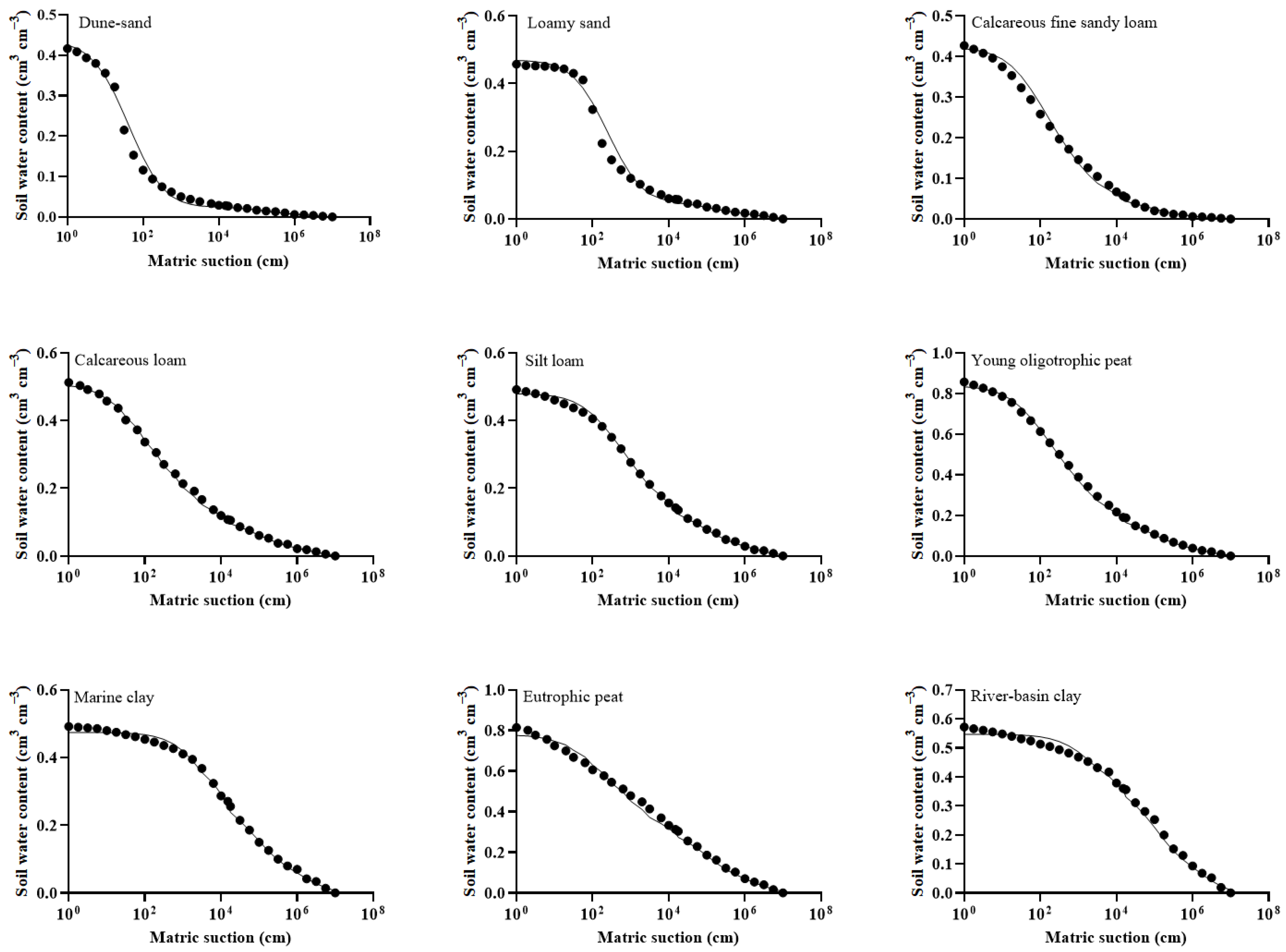
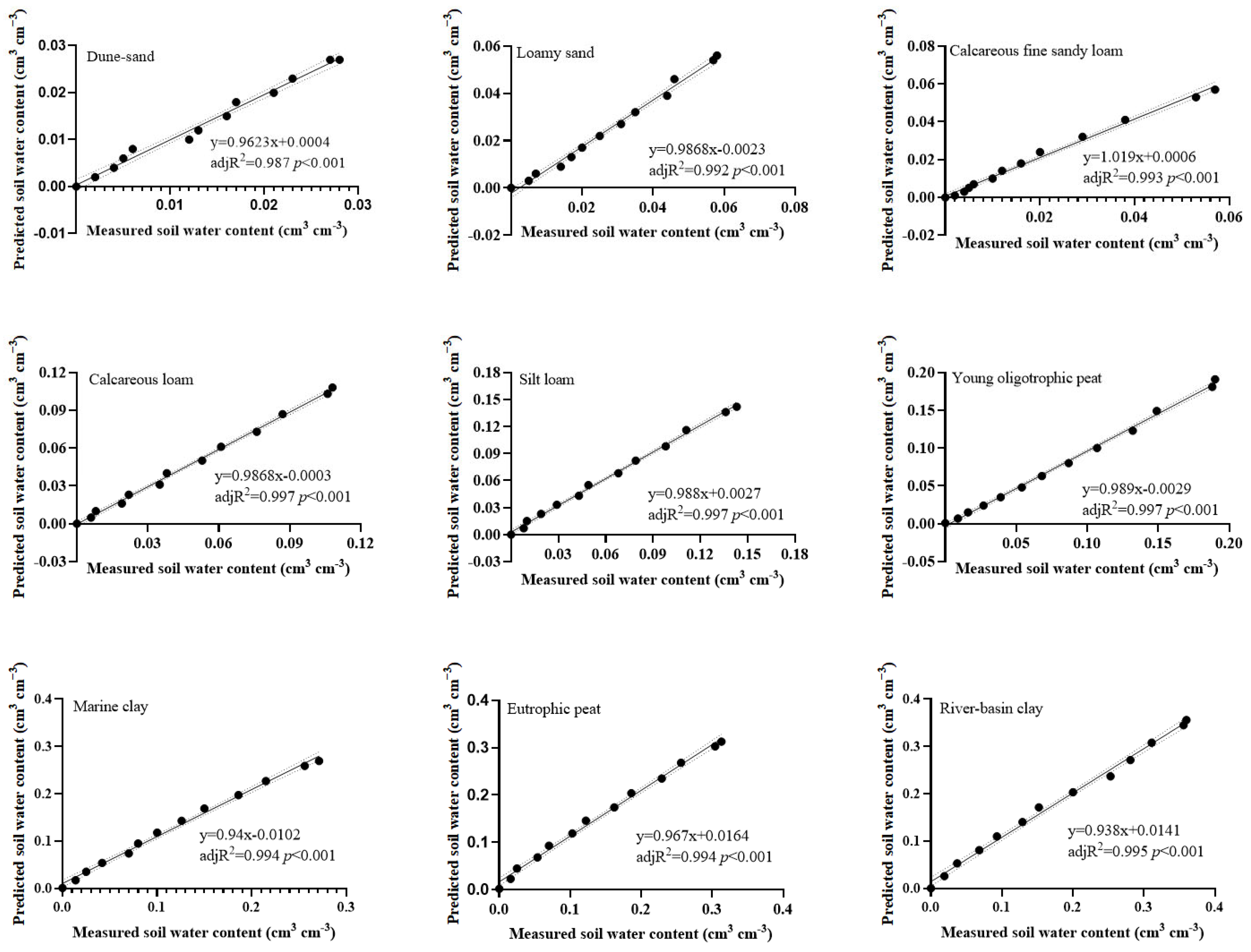
3.1. Test of the Three-Segmented Model for the Entire SWCC

Figure 1 illustrates the observed data and the fitted three-segmented models of the entire SWCC in the semilog coordinate system for nine different soils. In the figure, solid dots represent the observed SWD, while the solid black lines represent the fitted three-segmented model of the entire SWCC. The three-segmented model provides continuous and smooth curves from saturation to oven dryness by satisfactorily fitting the SWD for the nine soils. As shown in Figure 1, the fitted models of the entire SWCC closely match the SWD for all nine soils. For the calcareous loam, silt loam, and young oligotrophic peat soil samples, the goodness of fit values of the three-segmented SWCC models are almost the same. Thus, the adjR² values of calcareous loam, silt loam, and young oligotrophic peat are 0.998, 0.998, and 0.999, respectively, and the RMSE values are 0.007, 0.008, and 0.013 cm³ cm⁻³, respectively. For the other six soil retention datasets, the fitting performances of the three-segmented model are also good. As

Table 1. Fitting results of three-segmented model of the entire SWCC for nine soils.

Soil	θS	θR	θMH	θADC	ha	m	ω	λ	adjR2	RMSE
	cm3 cm−3				cm					cm3 cm−3
Dune sand	0.430	0.023	0.023	0.004	30	0.917	0.432	0.800	0.993	0.011
Loamy sand	0.469	0.043	0.046	0.010	146.7	0.938	0.401	0.740	0.991	0.016
Calcareous fine sandy loam	0.420	0.000	0.038	0.004	55	0.380	0.600	0.740	0.992	0.013
Calcareous loam	0.505	0.000	0.087	0.013	25	0.246	0.484	0.680	0.998	0.007
Silt loam	0.479	0.000	0.111	0.016	165	0.278	0.494	0.640	0.998	0.008
Young oligotrophic peat	0.835	0.029	0.149	0.021	50	0.35	0.498	0.540	0.999	0.013
Marine clay	0.474	0.000	0.215	0.034	1849	0.273	0.470	0.505	0.997	0.010
Eutrophic peat	0.777	0.000	0.256	0.040	39	0.165	0.472	0.502	0.992	0.022
River-basin clay	0.547	0.000	0.311	0.052	936	0.159	0.456	0.430	0.992	0.016

presents, the adjR² values of the nine soils are notably high, ranging from 0.991 to 0.999. Furthermore, their RMSE values are comparatively low, with a range of 0.007 to 0.022 cm³ cm⁻³.

As can be seen from Figure 1, the fitting SWCCs for dune sand and loamy sand exhibit a better match with the SWD in the range of 10^4.5 ≤ h ≤ 10^7.0 cm than in the range of 0 ≤ h ≤ 10^4.5 cm. Thus, it was necessary to further analyze the accuracy of the wet end model, air-dried end model, and oven-dried end model. The adjR² and RMSE for these three models were therefore calculated separately. Figure 2 displays the adjR² and RMSE for the wet segment model and air-dried segment model of the nine soils. As shown in Figure 2a,b, the adjR² values of the wet segment model for the nine soils varied between 0.944 and 0.999, and the RMSE values ranged from 0.005 to 0.026 cm³ cm⁻³. As illustrated in Figure 2c,d, it was evident that the air-dried segment models for the nine soils exhibited a range of adjR² values between 0.967 and 0.995, with RMSE values varying between 0.001 and 0.014 cm³ cm⁻³. This indicates that the air-dried segment model provides a better description of the SWCC in the range of 10^4.5 ≤ h ≤ 10^6.5 than the wet segment model does in the range of 0 ≤ h ≤ 10^4.5.

The oven-dried segment models for the nine soil samples had adjR² = 1 and RMSE = 0. This is because the oven-dried segment SWCC in this study only includes data points at 10^6.5, 10^6.75, and 10^7.0 cm. According to the oven-dried segment model, the precise anchoring points are at h_ADC = 10^6.5 cm (θ_ADC) and h_Z = 10^7.0 cm (θ_Z = 0). An appropriate adjustable fitting parameter λ value ensures that the fitted model accurately calculates the θ value at h = 10^6.75 cm, which is in exact agreement with the measured value. Therefore, the fitted values of θ corresponding to h = 10^6.5, 10^6.75, and 10^7.0 cm are exactly equal to the observed values. Thus, the fitted SWCC closely matches the observed SWD within the range of 10^6.5 ≤ h ≤ 10^7.0 cm.

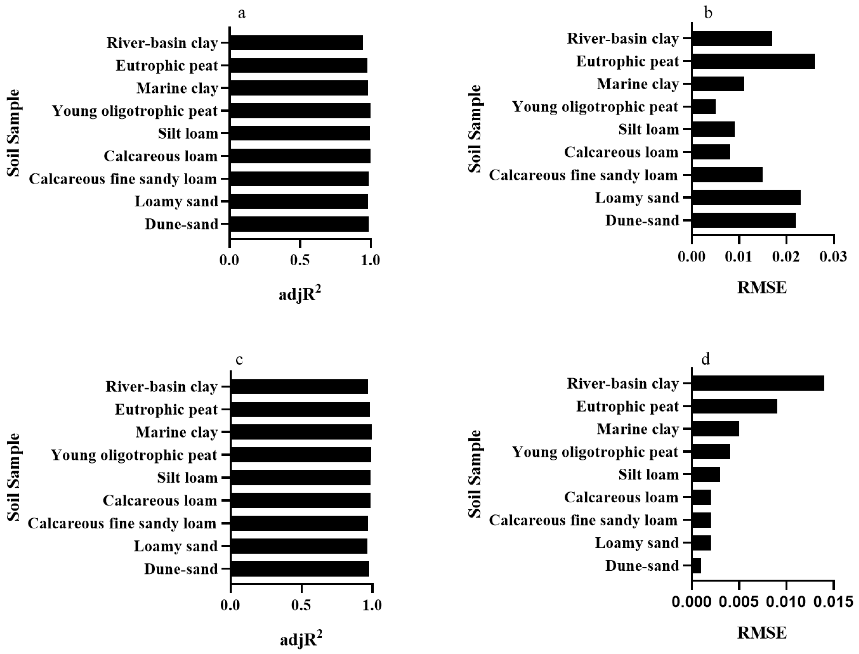
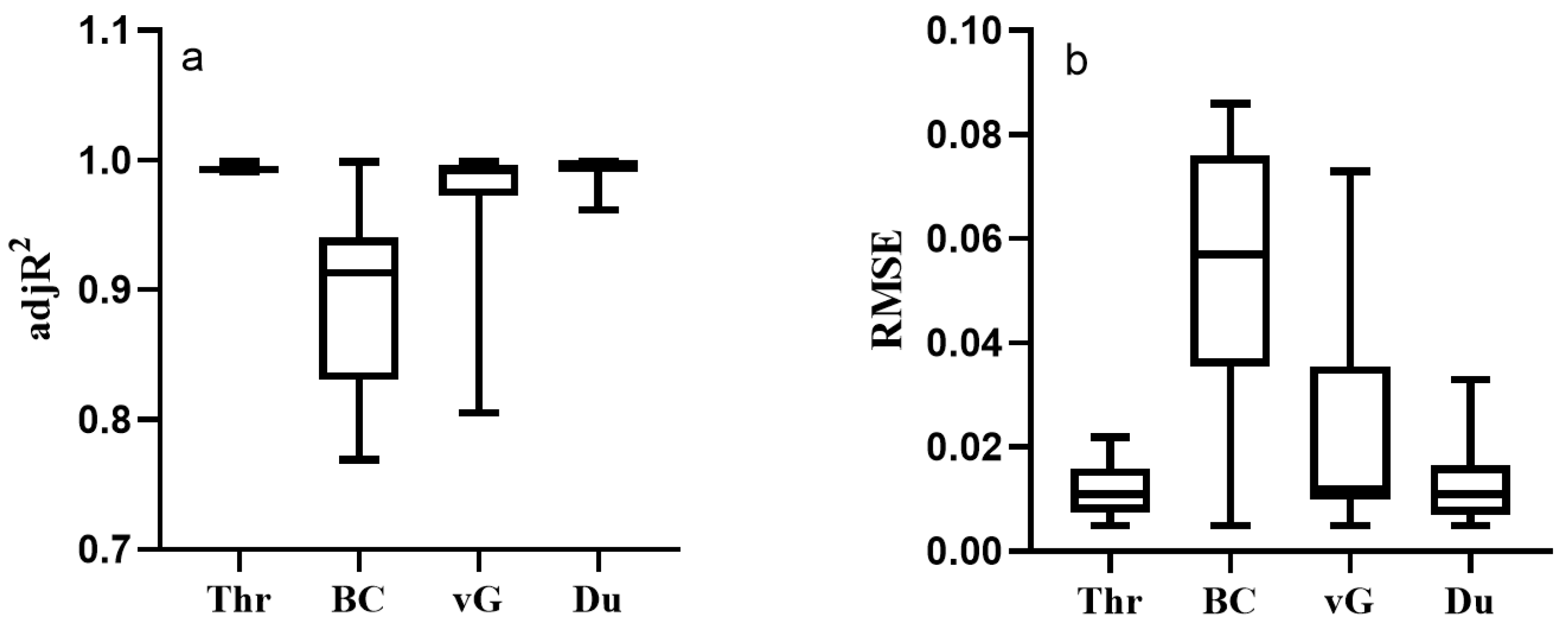
3.2. Comparison of SWCC Models

To evaluate the behavior of the three-segmented model proposed in this study, we compared it with three additional popular SWCC models. The expressions and parameters of the seven SWCC models are listed in

Table 2. Three SWCC models for comparison.

SWCC Model	Function	Parameters	Reference
BC model	θ = (h/hd)−β(θS − θR) + θR	θR, hd, β	[1]
vG model	θ = [1 + (αh)N]1/(N−1)(θS − θR) + θR	θR, α, N	[3]
Du model	θI = [1 + (αh)N]1/(N−1)(θS − θR) + θR (0 ≤ h ≤ ha) θII = (hd/h)βθS          (ha ≤ h ≤ hb) θIII = $\frac{{\log }_{10}{\mathrm{h}}_{\mathrm{Z}}-{\log }_{10}\mathrm{h}}{{\log }_{10}{\mathrm{h}}_{\mathrm{Z}}-{\log }_{10}{\mathrm{h}}_{\mathrm{b}}}{\mathsf{\theta }}_{\mathrm{b}}$        (hb ≤ h ≤ hZ)	θR, N, α, β, hZ, hb, θb	[16]

. The Brooks–Corey (BC) model [1] and van Genuchten (vG) model [3] are traditional models for describing the SWCC between θ_S and θ_R and are very popular. The Du model [16] is a three-segmented model, which is superior to other segmented models such as the Rossi and Nimmo model [15], the Peter model, the Zhang model [23], the DG model [29], and the Webb model [11], based on the research of Du [16].

As shown in Figure 3, the adjR² and RMSE were employed to evaluate and compare the performances of the three-segmented model and the three other SWCC models. Although the maximum adjR² value was close to 1 and the 25th percentile was greater than 0.80 for each model (Figure 3a), the variations in the adjR² values of the models were different. The adjR² for the three-segmented model only varied between 0.99 and 1.00. The 25th and 75th percentiles of the adjR² values for the Du model were similar to those of the three-segmented model, but the range of the minimum to the maximum adjR² values of the Du model was greater than that of the three-segmented model. The BC model, which is a traditional single-segment model, had the largest adjR² range, with a minimum of 0.769 and a maximum of 0.999. The adjR² values of the vG model ranged from 0.805 to 0.999. The results indicate that the three-segmented model proposed in this study slightly surpasses the Du model in describing the observed soil water retention data, and that it explains these data more effectively than single-segment models such as the BC and the vG models.

Figure 3b illustrates the RMSE variations of the four SWCC models. The minimum RMSE value of each model was close to 0, but the maximum varied greatly. The maximum RMSE values for the three-segmented model proposed here and the BC, vG, and Du models were 0.022, 0.086, 0.073, and 0.033 cm³ cm⁻³, respectively. The 75th percentiles of these four models were not greater than 0.08. Overall, the three-segmented model proposed in this study outperforms other models with a significantly smaller error.

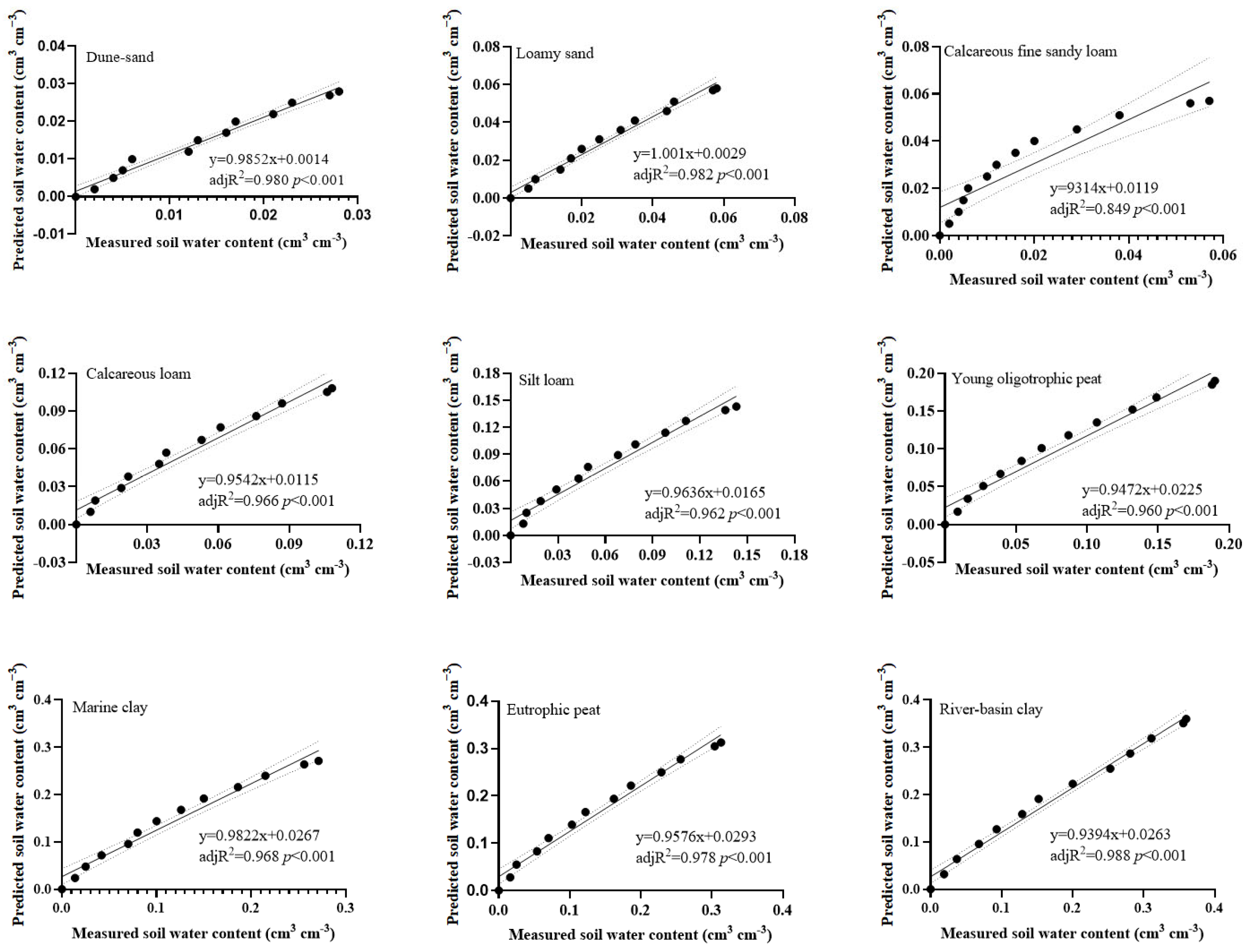
3.3. Predicting the Soil Water Content within the Interval of 0 ≤ θ ≤ θ_PWP

Equation (18) was fitted using SWD from the following four points: h = 10^3.75, 10^4.0, 10^4.18, and 10^7.0 cm. The predicted values of θ in the matric suction range of 10^4.18 ≤ h ≤ 10^7.0 cm, as estimated using Equation (18), were plotted against the measured values in a linear relationship in Figure 3. Highly significant linear relationships were found between the predicted and measured θ values (Figure 4). In theory, if the slope of the linear equation is equal to 1.0, the y-intercept is equal to zero, and the adjR² is equal to 1, the predicted values should match the measured values exactly. As shown in Figure 4, the slopes of the linear equations for the nine soils ranged from 0.938 to 1.019, and the y-intercepts varied between −0.0102 and 0.0164, with adjR² values ranging from 0.993 to 0.997. This indicates that the predicted θ values from Equation (18) closely match the measured θ values. Therefore, it is feasible to use the method provided in this study to predict SWD in the range of 10^4.18 ≤ h ≤ 10^7.0 cm.

To evaluate the prediction obtained using Equation (18), we compared it with the logarithmic model proposed by Du (2020) [16]. The logarithmic model is expressed as follows:

$$\mathsf{\theta }=\frac{{\log }_{10}{\mathrm{h}}_{\mathrm{Z}}-{\log }_{10}\mathrm{h}}{{\log }_{10}{\mathrm{h}}_{\mathrm{Z}}-{\log }_{10}{\mathrm{h}}_{\mathrm{b}}}{\mathsf{\theta }}_{\mathrm{b}}$$

(22)

where θ (cm³ cm⁻³) is the soil water content, h (cm) is the matric suction, h_Z (cm) is the matric suction of oven-dried soil, and θ_b (cm³ cm⁻³) and h_b (cm) are adjustable parameters. According to the SWD in this study, the h_Z (cm) is equal to 10^7.0 cm, and θ_b = θ_PWP corresponds to h_b = 10^4.18 cm. A strong linear correlation was identified between the estimated and actual θ values, as depicted in Figure 5. The slopes of the linear regression equations for the nine soils spanned from 0.9314 to 1.001, while the y-intercepts fluctuated from 0.0014 to 0.0293 (Figure 5). The adjR² values shown in Figure 5 vary between 0.849 and 0.988.

A comparative analysis of the slopes, y-intercept values, and adjR² values presented in Figure 4 and Figure 5 reveals that Equation (18) exhibits a narrower range of adjR² values, a tighter range of slopes, and smaller y-intercepts compared to Equation (22). Considering these points, it is reasonable to conclude that Equation (18) offers enhanced predictive accuracy for the soil water content within the interval of 10^4.18 < h < 10^7.0 cm than Equation (22).

It is crucial to note that while Equation (18) exhibits a high degree of predictive accuracy, it lacks inherent physical interpretability. This is because the fitting parameters of Equation (18), as listed in

Table 3. Fitting results of Equation (18).

Soil	θc	θd	he	γ	adjR2	RMSE
	cm3 cm−3		cm			cm3 cm−3
Dune sand	0.163	−0.028	0.104	0.104	0.992	0.003
Loamy sand	0.654	−0.022	0.229	0.194	0.971	0.012
Calcareous fine sandy loam	2.896	−0.004	1.169	0.408	0.993	0.007
Calcareous loam	1.229	−0.037	0.473	0.209	0.997	0.008
Silt loam	1.267	−0.064	0.474	0.180	0.996	0.012
Young oligotrophic peat	2.675	−0.029	31620	0.35	0.999	0.005
Marine clay	1.530	−0.24	0.294	0.115	0.982	0.042
Eutrophic peat	1.302	−0.407	0.730	0.087	0.983	0.051
River-basin clay	1.230	−0.689	1.131	0.064	0.992	0.042

, lack physical meaning. For example, the parameter θ_d is less than zero, and θc is greater than 1.0. Therefore, Equation (18) can only be used to predict θ in the range of 10^4.18 ≤ h ≤ 10^7.0 cm and cannot be used to describe the SWCC. In practical applications, Equation (18) is initially employed to predict SWD within the range of 10^4.18 < h < 10^7.0 cm. Subsequently, these predicted SWD can be used to fit the SWCC with the air-dried and oven-dried segment models.

4. Discussion

The entire SWCC describes the SWD across the full range from saturation to oven dryness [13,16,17,18]. The h corresponding to oven-dried soil is referred to as 10^7.0 cm in this study. This value is reasonable based on the calculations of Equations (1) and (2). For oven-dried soil, T = 378 K (105 °C) and 288K ≤ Tr ≤ 298K and 0.2 ≤ f ≤ 0.7. The calculation using Equations (1) and (2) yields an approximate value of h as 10^7.0 cm [18]. The θ value of oven-dried soil (θ_Z) is considered zero. This does not imply that there is no water in the oven-dried soil, but rather indicates that the water remaining in the soil after equilibrium at 105 °C has not been expelled. Consequently, at this point, the θ calculated according to Equation (16) is equal to zero.

θ_MH is referred to as the maximum θ of air-dried soil, which characterizes the boundary between the wet segment model and the air-dried segment model. θ_MH is defined as the maximum amount of water that air-dried soil particles can absorb from an environment close to water vapor saturation [25]. Thus, it is reasonable to use θ_MH as the maximum θ of air-dried soil.

The dividing point between the air-dried segment and the oven-dried segment is anchored at θ_ADC, corresponding to h = 10^6.5 cm, which describes the minimum θ value of air-dried soil. The relative air humidity corresponding to θ_ADC is 10% (0.1) at room temperature. Generally, it is difficult for the relative air humidity to drop to 10% at room temperature. Therefore, defining θ_ADC as the minimum θ of air-dried soil is theoretically reasonable, as the θ of air-dried soil usually exceeds θ_ADC, corresponding to h less than 10^6.5 cm.

The SWCC encompasses both the water adsorption and water release functions. In this study, the two anchor points of the three-segmented model are fixed at θ_MH and θ_ADC, which represent the maximum and minimum θ values of air-dried soil, respectively. Consequently, the three-segmented model of the SWCC proposed in this research falls within the category of the water release function.

5. Conclusions

By introducing segmented models for the wet, air-dried, and oven-dried segments, this study successfully describes the SWCCs from saturation to oven dryness. These models not only independently describe the soil moisture characteristics within their respective segments but also provide a continuous and accurate description of the entire moisture range when combined. The adjR² values of the three-segmented models for nine soils were consistently above 0.991, and the RMSE values did not exceed 0.022 cm³ cm⁻³.

The connection point between the wet segment model and the air-dried segment model is anchored at h = 10^4.5 cm, corresponding to θ_MH. θ_MH has a clear physical significance and is widely used in soil moisture research. Therefore, the connection point between the wet segment and air-dried segment models is not only an adjustable parameter but has a definite physical meaning. The connection point between the air-dried segment model and the oven-dried segment model is anchored at h = 10^6.5 cm for θ_ADC. θ_ADC is considered to represent the water content of air-dried soil at a relative humidity of 10% at room temperature. This perspective is proposed in this study and carries a degree of arbitrariness. Thus, further research is needed in the future to validate the feasibility of θ_ADC as a theoretical value for the minimum water content of air-dried soil. Overall, the first and second junction points of the three-segmented model for the entire SWCC are anchored at θ_MH and θ_ADC, respectively, providing new insights for understanding and applying SWCCs.

The prediction methods proposed in this research show high accuracy in predicting the soil moisture content in the high suction range, which is significant for reducing experimental workloads and improving work efficiency. This provides a new means for obtaining SWD in the high suction range.

References

1. Brooks, R.H.; Corey, A.T. Hydraulic Properties of Porous Media and Their Relation to Drainage Design. Trans. ASAE 1964, 92, 26–28. [Google Scholar]
2. Campbell, G. A simple method for determining unsaturated conductivity from moisture retention data. Soil Sci. 1974, 117, 311–314. [Google Scholar] [CrossRef]
3. Van Genuchten, M.T. A closed-form equation for predicting the hydraulic conductivity of unsaturated soils. Soil Sci. Soc. Am. J. 1980, 44, 892–898. [Google Scholar] [CrossRef]
4. Ikechukwu, A.F.; Hassan, M.M.; Moubarak, A. Resilient modulus and microstructure of unsaturated expansive subgrade stabilized with activated fly ash. Int. J. Geotech. Eng. 2021, 15, 915–938. [Google Scholar] [CrossRef]
5. Onyelowe, K.C.; Mojtahedi, F.F.; Azizi, S.; Mahdi, H.A.; Sujatha, E.R.; Ebid, A.M.; Darzi, A.G.; Aneke, F.I. Innovative Overview of SWRC Application in Modeling Geotechnical Engineering Problems. Designs 2022, 6, 69. [Google Scholar] [CrossRef]
6. Terleev, V.V.; Mirschel, W.; Badenko, V.L.; Guseva, I.Y. An improved Mualem–Van Genuchten method and its verification using data on Beit Netofa clay. Eurasian Soil Sci. 2017, 50, 445–455. [Google Scholar] [CrossRef]
7. Kuang, X.; Jiao, J.J. A new equation for the soil water retention curve. Eur. J. Soil Sci. 2014, 65, 584–593. [Google Scholar] [CrossRef]
8. Richards, L.A.; Weaver, L.R. Fifteen-atmosphere percentage as related to the permanent wilting point. Soil Sci. 1943, 56, 331–339. [Google Scholar] [CrossRef]
9. Mualem, Y. A Catalogue of the Hydraulic Properties of Unsaturated Soils; Technical Report; Israel Institute of Technology: Haifa, Israel, 1976; pp. 28–70. [Google Scholar]
10. Vogel, T.; Cislerova, M. On the reliability of unsaturated hydraulic conductivity calculated from the moisture retention curve. Transp. Porous Media 1988, 3, 1–15. [Google Scholar] [CrossRef]
11. Webb, S.W. A simple extension of two-phase characteristic curves to include the dry region. Water Resour. Res. 2000, 36, 1425–1430. [Google Scholar] [CrossRef]
12. Silva, O.; Grifoll, J. A soil-water retention function that includes the hyper-dry region through the BET adsorption isotherm. Water Resour. Res. 2007, 431, 398–408. [Google Scholar] [CrossRef]
13. Groenevelt, P.H.; Grant, C.D. A new model for the soil-water retention curve that solves the problem of residual water contents. Eur. J. Soil Sci. 2004, 55, 479–485. [Google Scholar] [CrossRef]
14. Ciocca, F.; Lunati, I.; Parlange, M.B. Effects of the water retention curve on evaporation from arid soils. Geophys. Res. Lett. 2014, 41, 3110–3116. [Google Scholar] [CrossRef]
15. Rossi, C.; Nimmo, J.R. Modeling of soil water retention from saturation to oven dryness. Water Resour. Res. 1994, 30, 701–708. [Google Scholar] [CrossRef]
16. Du, C. A novel segmental model to describe the complete soil water retention curve from saturation to oven dryness. J. Hydrol. 2020, 584, 124649. [Google Scholar] [CrossRef]
17. Koorevaar, P.; Menelik, G.; Dirksen, C. Elements of Soil Physics; Elsevier: Amsterdam, The Netherlands, 1983. [Google Scholar]
18. Chi, C. Two Models to Describe the Entire Soil Water Retention Curve. Eurasian Soil Sci. 2023, 56, 447–452. [Google Scholar] [CrossRef]
19. Fredlund, D.G.; Xing, A. Equations for the soil-water characteristic curve. Can. Geotech. J. 1994, 31, 521–532. [Google Scholar] [CrossRef]
20. Ross, P.J.; Williams, J.; Bristow, K.L. Equation for extending water-retention curves to dryness. Soil Sci. Soc. Am. J. 1991, 55, 923–927. [Google Scholar] [CrossRef]
21. Fayer, M.J.; Simmons, C.S. Modified soil water retention functions for all matric suctions. Water Resour. Res. 1995, 31, 1233–1238. [Google Scholar] [CrossRef]
22. Morel-Seytoux, H.J.; Nimmo, J.R. Soil water retention and maximum capillary drive from saturation to oven dryness. Water Resour. Res. 1999, 35, 2031–2041. [Google Scholar] [CrossRef]
23. Zhang, Z.F. Soil Water Retention and Relative Permeability for Conditions from Oven-Dry to Full Saturation. Vadose Zone J. 2011, 10, 1299–1308. [Google Scholar] [CrossRef]
24. Tuller, M.; Or, D. Water films and scaling of soil characteristic curves at low water contents. Water Resour. Res. 2005, 41, W09403. [Google Scholar] [CrossRef]
25. Guan, L. General Soil Science, 2nd ed.; Agricultural University Press: Beijing, China, 2016. [Google Scholar]
26. Smagin, A.V. Thermogravimetric determination of specific surface area for soil colloids. Colloid J. Russ. Acad. Sci. 2016, 78, 391–396. [Google Scholar] [CrossRef]
27. Smagin, A.V. Thermodynamic Concept of Water Retention and Physical Quality of the Soil. Agronomy 2021, 11, 1686. [Google Scholar] [CrossRef]
28. Schofield, R.K. The pF of the water in soil. Trans. 3rd Int. Congr. Soil Sci. 1935, 2, 37–48. [Google Scholar]
29. Vanderlinden, K.; Pachepsky, Y.A.; Pederera-Parrilla, A.; Martínez, G.; Espejo-Pérez, A.J.; Perea, F.; Giráldez, J.V. Water Retention and Preferential States of Soil Moisture in a Cultivated Vertisol. Soil Sci. Soc. Am. J. 2017, 81, 1–9. [Google Scholar] [CrossRef]
Figure 1. Fitting results of three-segmented model of the entire soil–water characteristic curve (SWCC) for nine soils.
Agronomy 14 00707 g001
Figure 2. Values of the adjusted coefficient of determination (adjR2) and root mean square error (RMSE) of the wet segment model (a,b) and the air-dried segment model (c,d) for nine soils.
Agronomy 14 00707 g002
Figure 3. Comparison of the three-segmented SWCC model and other segmented SWCC models in terms of adjR2 (a) and RMSE (b). The horizontal solid line in each box signifies the median value, and the bottom and top of the box represent the 25th and 75th percentiles, respectively. The error bars represent the range from the minimum to the maximum values. Thr (three-segmented model proposed in this study), BC (Brooks–Corey model), vG (van Genuchten model), and Du (three-segmented model proposed by Du, 2020 [16]).
Agronomy 14 00707 g003
Figure 4. Relationships between the measured soil water content and the soil water content predicted using Equation (18) proposed in this study. The dots in the figure represent the actual measured values of soil water content, the solid lines indicate the linear regression between the measured soil water content and the soil water content predicted using Equation (18), and the dashed lines represent the prediction intervals.
Agronomy 14 00707 g004
Figure 5. Relationships between the measured soil water content and the soil water content predicted using the logarithmic model proposed by Du (2020) [16].The dots in the figure represent the actual measured values of soil water content, the solid lines indicate the linear regression between the measured soil water content and the soil water content predicted using the logarithmic model proposed by Du (2020) [16], and the dashed lines represent the prediction intervals.
Agronomy 14 00707 g005